


Abstract
Machine learning is increasingly used for spacecraft telemetry monitoring, fault diagnosis, health assessment, mission planning, visual navigation, and execution review. In space missions, explainability is a foundation of trustworthy artificial intelligence because engineers must understand the evidence behind model outputs before incorporating them into operational decisions. Explainability should therefore transform internal model computations into evidence that engineers can inspect during mission execution and integrate into an intuitive mental model of spacecraft state, model rationale, and possible action consequences. Such evidence may include channel–time patterns, rule paths, prototype events, active constraints, or subsystem propagation hypotheses. It must remain traceable to the model, consistent with spacecraft modes and physical constraints, and usable in reviewable decisions. This review distinguishes the mechanism that generates an explanation from the strength of its spacecraft validation. It examines interpretable-by-design models and six post-hoc families, separating direct spacecraft evidence from methods transferable from adjacent domains. A V0–V5 scale describes evidence ranging from generic experiments to measured mission-support benefit. Finally, the review discusses the Open-Box method and examines how exact and consistent regional representations may be relevant to piecewise-linear network families within verified operating regions.
1. Introduction
The operational purpose of explainability in spaceflight is to make a machine learning decision visible in a form that an engineer can recognize while the mission is unfolding. A score, class label, or recommended action does not by itself create understanding. The system should expose an evidence object, such as a channel-time pattern, a rule path, a matched historical event, an active constraint, or a candidate propagation path. The engineer can then connect that object with the current spacecraft mode, subsystem state, command history, and possible consequence. This connection supports an intuitive mental model of what the spacecraft is doing, why the model responded, and what should be inspected next. Explainability in this review therefore refers to operationally usable cognition rather than visual presentation alone. Existing spacecraft studies already produce several parts of that cognitive picture. GalaxAI combines telemetry preparation, anomaly analysis, and interpretable inspection in a spacecraft-oriented toolbox [1]. Cuellar et al. attach Local Interpretable Model-agnostic Explanations (LIME) to a telemetry anomaly classifier and identify the variables that support a single alarm [2]. Kricheff et al. use Shapley Additive Explanations (SHAP) and layer-wise relevance propagation (LRP) to distribute anomaly and forecast scores across satellite telemetry channels [3]. Diagnosis studies contribute a complementary engineering picture. Chen et al. use causal discovery to organize candidate roots of on-orbit anomalies [4]. Their later hierarchical method connects local anomaly evidence with upstream variables [5]. Schefels et al. place causal inference in an operational anomaly investigation workflow [6]. Di et al. retain satellite power-system topology through interpretable graph filtering [7]. These studies expose local model evidence that can be placed beside the corresponding telemetry event.
Planning and execution studies are fewer, but they expose requirements that telemetry attribution alone does not cover. Powell and Riccardi use computational argumentation to explain why an autonomous scheduler selected one action over another [8]. Bhamidipati et al. reconstruct onboard decisions and execution anomalies from downlinked records [9]. Candela et al. combine outcome prediction with explanations intended for autonomous mission operations [10]. In these cases, the useful evidence is a constraint, rejected alternative, or execution trace rather than a channel ranking. The literature therefore cannot be compared through a single notion of interpretability.
General explainable artificial intelligence (XAI) surveys provide the vocabulary for organizing this diversity [11,12,13,14,15].
Two questions guide this review. The first asks how a method produces an explanation. SHAP, for example, assigns additive feature contributions and can be implemented in model-agnostic or model-specific forms [16]. The second asks where the resulting evidence has been tested and what decision it can support. Trusted-autonomy research frames this second question through mission constraints, communication limits, human oversight, and assurance [17]. Operational studies of autonomous spacecraft add the ground processes needed to review onboard decisions [18]. Broader space-science XAI work offers useful transferable methods but often stops short of spacecraft operations [19]. Keeping the two questions separate prevents a mature algorithm from being mistaken for a mature operational capability.
The review is structured around that separation. Section 2 defines the operational scope and evidence language. Section 3 explains the internal logic of the principal methods and gives more space to mechanisms that can produce traceable temporal, rule-based, or structural evidence. Section 4 distinguishes spacecraft-focused studies from transferable work without repeating that distinction for every method. Section 5 presents the V0–V5 evidence scale and claim-specific evaluation. Section 6 identifies engineering priorities and discusses exact and consistent regional representations alongside the Open-Box method [20] for piecewise-linear network families. Section 7 summarizes why precise explanation is a mission requirement rather than an optional visualization.
The synthesis in Section 2, Section 3, Section 4 and Section 5 consolidates the reviewed literature by separating explanation mechanisms, evidence objects, operational contexts, and available validation evidence. The V0–V5 scale in Section 5 is proposed in this review as a claim-level evidence-classification framework. Section 6.4 discusses the Open-Box method reported by Mozolewski et al. [20] and examines conditions under which rule aggregation and exact regional representations may be relevant to spacecraft operations; it does not claim a new Open-Box architecture or a spacecraft-validated implementation.
2. Scope and Organizing Logic
2.1. Review Search and Selection Approach
This review used a targeted and transparent search-and-selection approach. ScienceDirect (Elsevier), IEEE Xplore, and Google Scholar were searched and updated through 16 September 2026. The search covered publications issued from 2016 to 2026, which is also the publication-date range of the final cited corpus. Representative search combinations paired “spacecraft”, “satellite”, or “space operations” with “explainable AI”, “explainable machine learning”, “interpretability”, “XAI”, “telemetry anomaly detection”, “fault diagnosis”, “autonomous planning”, or “onboard autonomy”. Approximately 150 records were initially identified. After duplicate removal, title-and-abstract screening, and full-text assessment, 83 references were retained in the final review; 18 spacecraft-focused studies were retained for the core comparative synthesis. A study was classified as spacecraft-focused when its explanation was connected to a spacecraft or ground-segment operational task. A study was classified as transferable when it supplied a relevant explanation mechanism without direct evidence for a spacecraft operational decision.
2.2. Scope and Classification Criteria
Studies were included as spacecraft-focused when their explanation was connected to a spacecraft or ground-segment operational task, including telemetry monitoring, fault diagnosis, health assessment, planning, navigation, execution review, or a representative engineering environment. Studies from remote sensing, space science, or adjacent safety-critical domains were retained as transferable only when they contributed a relevant explanation mechanism but did not establish support for a spacecraft operational decision. Data source alone did not determine classification; the deciding criterion was the relationship between the explanation and an operational engineering task. An aerospace study was classified as transferable when its explanation evidence was generated outside a spacecraft or ground-segment operational task; it was classified as spacecraft-focused only when the study directly linked the explanation to such a task.
The following analysis distinguishes interpretability, explainability, faithfulness, and causal explanation because they support different parts of an intelligent spacecraft-operation workflow. Interpretability is a property of a model representation: a prediction path is directly inspectable through, for example, coefficients, rules, states, concepts, or prototypes. An intrinsically interpretable model makes that representation available by design, provided that its variables, preprocessing, rule priorities, and mode logic are documented. Before an interpretable representation is used operationally, its stated conditions and predicted relations must be checked against spacecraft physics, configuration, telemetry provenance, command history, and the active mission mode. A conflict does not automatically invalidate the representation; it must be recorded, investigated, and supported by evidence such as a mode transition, sensor fault, unmodelled coupling, or data-quality issue. Within a verified operating region, the rule or trace can then be followed as a controlled decision-support procedure, while the operator retains responsibility for judging exceptions, uncertainty, and safety consequences.
Explainability is the capability of a model-and-workflow combination to produce, present, and preserve task-relevant evidence about a specified output or decision for a specified user. The evidence object may be a channel-time attribution, a response curve, a local rule, a prototype event, a concept state, a feasible counterfactual, a subsystem path, or a planned-versus-executed trace. Its content, intended user, operating mode, data window, predictor and explainer version, validity region, and uncertainty must be stated in advance. Its adequacy is judged against the operational question: alarm triage requires evidence about the relevant channels and event window; diagnosis requires a trace or mechanism hypothesis that can be checked against engineering records; and replanning requires feasible alternatives, constraints, and a replayable decision trace. A black-box predictor can therefore be part of an explainable operational system when this evidence is generated reproducibly, evaluated under its declared conditions, linked to the relevant task, and made available in a form that qualified personnel can interpret and challenge.
Faithfulness concerns whether the stated evidence object represents the behavior of the predictor that it claims to explain. It is evaluated against the predictor, not against an operator’s intuition or physical plausibility alone. A physically plausible attribution can be unfaithful if it does not reproduce the predictor’s dependence on the relevant channels. Conversely, a faithful rule may show that the predictor relies on an inappropriate proxy, omits a relevant mode condition, or behaves undesirably in a declared region. Faithfulness therefore establishes correspondence to the model; engineering usefulness requires the additional demonstration that the evidence improves a defined task, such as diagnosis, triage, replanning, audit, or operator performance, without violating latency, resource, safety, and configuration constraints. Tests must match the object and claim: local fidelity and coverage for a surrogate, deletion or perturbation behavior for an attribution, agreement under a declared reachable domain for an extracted rule, stability across admissible modes and preprocessing versions, and task-level comparison against an appropriate baseline where operational use is intended.
Causal explanation addresses the further system-level question of whether a factor, relation, or intervention changes an operational outcome through a stated mechanism. This is stronger than showing a statistical association with a prediction or showing that an evidence object faithfully describes the predictor. Causal validity requires an explicit causal question, temporal ordering, treatment of confounding and commands, and evidence from intervention, replay, a validated simulator, or another engineering test capable of distinguishing cause from correlation. In spacecraft operations, a channel highlighted during an anomaly may be a symptom, a commanded transition, or a common response to an unobserved condition. The claim should therefore be stated as descriptive, predictive, faithful, operationally useful, or causal according to the evidence actually established.
This review uses intelligent spacecraft operations to denote the activities through which a spacecraft and its ground segment monitor state, detect abnormal behavior, diagnose faults, estimate health or risk, select actions, support navigation, and reconstruct autonomous execution. The definition is deliberately narrower than “AI in space.” A remote-sensing classifier is relevant only when it exposes an explanation that can be tied to an operational decision. A learning controller is included only when its internal logic, policy rationale, or decision evidence is made inspectable. This boundary keeps the discussion centered on mission operations, where an explanation must enter a chain of engineering judgment rather than remain a visualization attached to a prediction.
Operational deployment should specify the predictive or decision model, the explanation mechanism, the user, and the operational task together. The evidence object is then presented in a form that the intended user can place into an operational mental model. The same output can serve one user and fail another. A developer may use a channel attribution to identify data leakage. A subsystem engineer needs the attribution grouped by component, time interval, and operating mode. A flight controller usually needs a smaller cognitive object: the affected subsystem, onset time, evidence that changed, confidence or rule validity, and the next inspection step. A mission planner asks which constraints were active, why an alternative was rejected, and whether another feasible action could achieve the objective. Method labels alone do not resolve these differences.
Spacecraft data also impose conditions that are easy to overlook in generic XAI experiments. Telemetry channels are coupled through control loops, protection logic, shared power buses, thermal paths, and command sequences. Their statistical meaning changes between sunlight and eclipse, safe mode and payload operation, or steady pointing and a maneuver. Sampling can be irregular. Missing packets are common. The spacecraft processor may have little memory, and the ground team may receive only a selected event window. Onboard telemetry monitoring studies make latency and output size explicit design constraints [21], while knowledge-graph work shows that component topology and named relations can be part of the explanation itself [22]. An explanation that ignores these conditions may be mathematically valid for the learned model yet unusable in operations.
The review uses the term evidence object for the part of the model behavior that can be inspected and discussed. Examples include a channel-time pattern, a response curve, a local rule, an activation region, a prototype event, a concept state, a feasible counterfactual, a subsystem path, or a planned-versus-executed trace. This terminology is more precise than calling an entire model explainable. It also clarifies what must be evaluated. A heat map should be tested as a spatial or temporal attribution. A rule should be tested for fidelity, coverage, and complexity. A concept state needs semantic validation. A causal path requires temporal and engineering checks. The evaluation target follows the evidence object, not the graphic used to display it.
A second distinction concerns the strength of the claim attached to that evidence. Some explanations describe the model locally. Others imply a physical mechanism, a cause, or a safe action. These are different commitments. F-Fidelity tests whether an explanation changes in accordance with the model evidence that it is intended to represent [23]. Quantus implements a broad collection of explanation metrics [24], and later metric studies organize the relationship among faithfulness, robustness, complexity, and human interpretability [25]. Robustness-based aerospace evaluation adds another layer by testing learning-enabled behavior under controlled perturbations and failure conditions [26]. None of these assessments can be replaced by visual plausibility. Conversely, a physically plausible account still requires a check that it actually represents the model.
Two evidence tracks are maintained from this point onward. The first contains spacecraft-focused studies: mission telemetry, spacecraft simulators, engineering-representative tests, onboard experiments, or operational decision records. The second contains transferable methods developed on public or adjacent-domain data. Transferable work is valuable because the spacecraft literature does not yet cover every explanation mechanism. It is nevertheless kept separate from direct spacecraft evidence. Section 4 makes that distinction once at the application level, and later sections refer back to it rather than repeatedly labeling each method as validated or unvalidated.
The methodological taxonomy uses the stage at which interpretability enters the model and the dominant mechanism that produces the evidence object. Interpretable-by-design models expose coefficients, rules, states, concepts, or prototypes as part of the prediction path. Post-hoc methods inspect a trained model through response analysis, attribution, surrogate fitting, examples and counterfactuals, concepts and representations, or causal and knowledge structures. The categories are not rigid compartments. A prototype network may be interpretable by design, while retrieval from a black-box embedding is post-hoc. A causal graph may be embedded in the predictor or learned afterward. Scope, model dependence, data type, output form, user, and purpose are therefore treated as cross-cutting descriptors rather than additional top-level branches.
3. Methods That Matter for Spacecraft Operations
Figure 1 presents the organizing taxonomy. The left branch contains models whose inspectable structure participates directly in prediction. The right branch groups post-hoc mechanisms by the computation that produces the evidence object: response analysis, attribution, surrogate or rule fitting, example or counterfactual search, concept-level analysis, and causal or knowledge-structured reasoning. The discussion below follows the computation from input to output. For each family, it identifies what the method receives, what intermediate operations it performs, what evidence it returns, and how an engineer should read that evidence during a spacecraft task. The taxonomy is not a maturity ranking; application and validation evidence are examined separately in Section 4 and Section 5.
Figure 1.
Taxonomy of explainable machine-learning methods considered for intelligent spacecraft operations.
To facilitate comparison across methods, each family is assessed by the evidence object returned to the engineer, model dependence (intrinsic, model-agnostic, or model-specific), data and operating assumptions, and the principal operational limitation. Thus, a method is not treated as operationally mature merely because its algorithm is mature: coupled telemetry, mode changes, temporal continuity, reachable-state constraints, resource cost, and unsupported causal interpretation can each limit mission use.
3.1. Interpretable-by-Design Models and Response Analysis
Interpretable-by-design models remain the clearest option when a mission team can express the decision with a compact structure. A linear model follows a transparent sequence. First, preprocessing converts engineering quantities into the model inputs and records scaling, units, and missing-value treatment. Second, the model multiplies each input by a learned coefficient and adds an intercept. Third, a generalized linear model passes that sum through a known link function to obtain a probability, rate, or other target. The signed products show how each input moves the linear score for that sample. Engineers can inspect the coefficient sign, the contribution magnitude after scaling, and the final threshold that converts the score into a decision. The interpretation is reliable only when feature definitions remain stable; correlated telemetry channels can make several coefficient allocations fit the same data. Sparse and monotonic constraints can improve auditability by limiting the number of active terms or enforcing an engineering direction of response.
A generalized additive model retains this additive accounting but learns a separate nonlinear shape function for each input. The model first maps every feature value through its learned curve. It then adds the curve outputs, optional low-order interaction terms, and an intercept before applying the final link. The curve shows where the model is flat, sensitive, saturated, or non-monotonic. For example, a battery temperature function may have little effect within a nominal band and rise sharply near an operational limit. The engineer can reconstruct the prediction by reading the contribution from each curve at the observed value. Interactions need explicit treatment; a purely additive model cannot represent a temperature-current condition unless the interaction is included.
Decision trees and rule lists replace arithmetic decomposition with a path. A tree begins at the root, evaluates one named condition, follows the corresponding branch, and repeats the process until it reaches a leaf containing a class, probability, or regression value. The explanation is the ordered sequence of conditions that the sample satisfied. A rule list evaluates clauses in a declared order and returns the consequence of the first matching rule, so priority is part of the mechanism. These structures are directly reviewable only while they remain small. A tree with hundreds of leaves, a large ensemble, or a rule base with many overlapping clauses can recreate the opacity it was intended to avoid. Complexity control, stable variable names, explicit units, and links to real spacecraft quantities are therefore part of the model design rather than cosmetic reporting choices.
Satellite power-system diagnosis illustrates a multi-stage interpretable mechanism. The decision-theoretic rough-set stage first forms condition attributes from measured voltages, currents, temperatures, or status variables. It then compares samples that are indistinguishable under those attributes and divides the decision space into a lower region, a boundary region, and an upper or negative region. Samples in the lower region support a diagnosis with sufficient certainty. Samples in the boundary region remain ambiguous and should not be forced immediately into a hard class. Attribute reduction can remove redundant measurements while preserving the discernibility needed for the decision.
The Takagi-Sugeno stage then converts the retained variables into graded evidence [27]. Each premise variable enters one or more membership functions. Their membership degrees determine the firing strength of each fuzzy rule. The method normalizes those firing strengths, evaluates the local linear consequent attached to every active rule, and combines the consequents into the final diagnostic output. Engineers can therefore inspect the selected attributes, the shape and calibration of each membership function, the rules that fired, their relative weights, and the final weighted consequence. The mechanism is suitable when fault signatures overlap across modes, because it preserves uncertainty instead of hiding it in a single label. Maintenance remains demanding: a new mode can alter the rough-set partitions, membership functions, and rule interactions, so the rule base must be versioned and revalidated with the operating envelope.
State-space and temporal models can also be interpretable when their states have an engineering definition. The mechanism begins with a state variable that summarizes information not directly observed. A transition model predicts how that state should evolve from the previous time step, commands, and disturbances. A measurement model predicts the sensor values expected from the state. The filter or estimator compares those predictions with actual telemetry, computes a residual, and updates the state estimate and its uncertainty. A hidden-state or switching model may additionally calculate the probability of each operating mode and the probability of moving between modes. The useful explanation is not merely the latent vector. It is the sequence linking prior state, command, predicted measurement, residual, update, and mode probability.
An engineer can interpret this sequence when the states correspond to a sensor bias, wheel friction, thermal margin, battery condition, or another monitored quantity. The residual identifies what observation forced the update. The transition probability identifies whether the model interpreted the event as a mode change or a within-mode deviation. Confidence bounds show whether the estimate is well supported. The model loses its intrinsic interpretability when the latent state has no stable mapping to physical or operational variables. That mapping must be established across the mission modes in which the estimator will be used.
Self-explaining neural networks move interpretable structure into a differentiable prediction path [28]. The first component maps the raw input into a small set of concepts or basis functions. Depending on the design, these concepts may be fixed engineering quantities or learned functions of the telemetry. A second component computes relevance coefficients that can change with the input. The prediction layer multiplies each concept value by its local relevance coefficient and adds the terms through a locally linear aggregator. Training optimizes predictive loss together with regularizers that encourage concept stability, diversity, sparsity, or smooth local behavior. At inference time, the model returns the prediction, the concept values, and the local coefficients in the same forward pass.
The engineer reads the output in two stages: which concepts are active, and how strongly each active concept moves the decision at that input. Because the explainer is inside the predictor, no separate perturbation model has to approximate the network afterward. This reduces one source of predictor-explainer mismatch. It does not solve semantic control. Learned concepts may drift between datasets, two concepts may encode the same operational condition, and local coefficients can change sharply near a boundary. A spacecraft concept should therefore receive an engineering name only after examples, interventions, and mode-wise stability tests show what the concept represents.
Concept bottleneck models use a more explicit two-stage path [29]. Before training, the designer defines a concept vocabulary, for example low energy margin, excessive wheel momentum, image blur, or thermal drift. The concept encoder receives the original input and predicts a value or probability for each named concept. The target model then receives only those concept predictions, or a declared combination of concepts and residual features, and computes the final diagnosis, health estimate, or action. During inference, engineers inspect the concept vector before reading the target output. In intervention-enabled designs, they can replace an incorrect concept prediction with a verified value and run the second stage again. The change in the target output shows how the decision depends on that concept.
The bottleneck is useful only when it truly carries the predictive information. Training may use concept labels and target labels jointly, sequentially, or with auxiliary losses. Each choice affects concept accuracy and downstream performance. Information can bypass the intended bottleneck if unrestricted residual connections are present. An incomplete concept set can force the model to encode unlisted conditions in unstable proxies, while noisy labels can make the concept names misleading. Validation must therefore check concept accuracy, concept completeness, intervention behavior, and whether the target stage uses the bottleneck in the intended way. The concept display is part of the predictive chain, not a decorative panel added after the decision.
Prototype networks offer a different form of intrinsic evidence by grounding a decision in similarity [30]. ProtoPNet first passes the input through a feature extractor and produces a spatial latent map. It stores a set of learned prototype vectors associated with classes or concepts. The model compares every prototype with every latent patch, converts distance into similarity, and keeps the strongest match. A linear classification layer combines the prototype similarities into class scores. The explanation contains the input region that matched, the corresponding prototype, the similarity value, and the prototype’s contribution to the class score. Many implementations project a learned prototype onto a nearby training patch so the displayed prototype corresponds to a real example rather than an unconstrained latent vector.
ProtoTSNet adapts the same computation to multivariate time series [31]. It extracts candidate temporal subsequences from the encoded record, compares them with learned temporal prototypes, and identifies the time window that produces the highest similarity. The model then combines the prototype matches to obtain the class decision. For telemetry, the evidence can be a short wheel-current excursion, thermal drift, or power transient. An engineer should see the current window, the matched prototype window, the channels used in the similarity, the mission phase of the reference event, and the contribution of the match to the prediction. Provenance is essential. A visually convincing match is not operational evidence when the two windows came from incompatible modes, preprocessing versions, or subsystem states.
Model-response analysis asks how the trained output changes when one input or a structured group of inputs changes. Partial dependence follows a four-step computation. It selects a grid of values for one feature, replaces that feature with each grid value across the evaluation records, queries the model, and averages the resulting predictions. The curve is therefore a population-average response under a synthetic replacement operation. Individual conditional-expectation analysis performs the same replacements but retains one curve per record, which exposes subgroups and interactions hidden by the average. Accumulated local effects avoid replacing a feature far outside its observed relationships. They divide the supported feature range into intervals, estimate the model’s local prediction change within each interval, and accumulate those changes into a centered response curve.
Permutation importance uses a different logic. It first measures a baseline performance score, disrupts one feature or a structured feature group, reruns the predictor, and records the loss of performance. The decrease reflects dependence of predictive performance on that information under the chosen permutation scheme. Interaction measures compare the joint response of two or more variables with the sum of their separate responses. Together, these tools can expose thresholds, reversals, saturation, and interactions that are not visible in accuracy metrics. They describe the learned response surface rather than the cause of a physical event. For spacecraft data, the replacement, interval, or permutation operation must preserve mode and subsystem coupling; otherwise, the curve can be dominated by unreachable states.
Spacecraft use requires a structured version of response analysis. Varying one temperature while holding all currents, loads, modes, and commands fixed can create a state that the spacecraft cannot reach. A global thermal curve averaged across eclipse, sunlight, safe mode, and payload operation can also conceal the behavior that matters in each regime. Response curves should therefore be conditioned on mode, restricted to supported ranges, and grouped according to subsystem architecture. Useful groups include solar-array generation and battery variables, wheel speed and current, thermal-zone measurements, or planning resources and observation value. The grouping should follow engineering structure rather than whichever combination produces the cleanest plot.
Response analysis can serve several stages of the mission lifecycle. Before deployment, it helps identify implausible sensitivities and regions with sparse training support. During qualification, a simulator can sweep an admissible state range and compare the learned response with expected subsystem behavior. During operations, a local response curve can show whether an event lies near a learned threshold or at the edge of model support. These uses are related but not interchangeable. The development plot explores model behavior; the operational plot must also carry mode, data provenance, and uncertainty.
Compared with post-hoc approaches, interpretable-by-design models and response-analysis methods provide different evidence for spacecraft tasks. A transparent predictor or executable rule returns an inspectable decision path, coefficient, state transition, or firing trace; this evidence is inseparable from the model structure and can be audited only if preprocessing, rule priorities, and mode logic are versioned. Response analysis returns a sensitivity pattern rather than the decision path itself and is more readily applied to an existing predictor, but it depends on the perturbation range, feature dependence assumptions, and the validity of holding other spacecraft variables fixed. In coupled telemetry, an implausible perturbation can create an operational state that the spacecraft cannot reach. These methods are therefore strongest for design review, threshold inspection, and rule-based recovery when engineering variables and admissible operating ranges are explicit; they are weaker when hidden state, mode transitions, or unrecorded commands dominate the prediction.
3.2. Attribution Across Telemetry, Graphs, and Images
Feature attribution assigns a contribution or relevance score to an input feature, channel, time interval, graph node, or image region. Methods that produce similar heat maps can follow very different computations. The important distinction is the conservation or comparison rule used to move from the model output back to the input. The following mechanisms should therefore be interpreted separately rather than grouped only by display format.
Integrated Gradients starts by selecting a reference input that represents the absence or comparison state [32]. It creates a path from that reference to the observed input, usually a straight line. At a sequence of points along the path, it computes the gradient of the target output with respect to every input. It then numerically integrates those gradients and multiplies the result by the difference between the observation and the reference. The resulting attributions approximately sum to the change in output between the two endpoints. This completeness relation gives engineers an accounting check. Saturated gradients at the observation are less problematic because the method samples the whole path, but the path may still cross unrealistic spacecraft states. A mode-matched baseline and a physically admissible interpolation path are therefore central to the result.
Layer-wise relevance propagation begins with an ordinary forward pass and records the activations [33]. It initializes the output neuron with the score to be explained. Starting at the last layer, it redistributes that relevance to the neurons in the preceding layer according to a selected propagation rule. The rule uses activations and weights, often with stabilizing terms, to decide how much relevance each lower neuron receives. The procedure repeats layer by layer until relevance reaches the input channels. Many variants preserve an approximate conservation relation, so the input relevances sum to the explained output or to a defined part of it. The chosen rule matters near zero denominators, negative contributions, normalization layers, and multiplicative operations. A spacecraft study should report the exact rule at each layer and verify that conservation and sign behavior remain meaningful for the network architecture.
DeepLIFT also propagates information backward, but it explains differences from a reference activation rather than local derivatives [34]. The method first performs a forward pass for the reference and another for the observed input. It computes the activation difference at each neuron. Local multipliers describe how a difference in one neuron contributes to the difference in the next. A chain rule combines these multipliers through the network and assigns the output difference to the input differences. This approach can return nonzero contributions where the ordinary gradient is saturated. The result still depends on the reference and on how nonlinear or interacting operations are decomposed. DeepSHAP later uses this propagation logic with multiple background examples to approximate Shapley-style contributions.
Grad-CAM produces a spatial explanation from a convolutional layer [35]. The model first performs a forward pass and stores the selected feature maps. It then computes the gradient of the target class score with respect to every location in those maps. Spatial averaging turns each gradient map into one weight per feature map. The method forms a weighted sum of the feature maps, applies a rectifier, and upsamples the result to the input resolution. The heat map indicates regions associated with increasing the target score at that layer. Its resolution is limited by the chosen feature map, and the rectifier suppresses negative evidence. Changing the layer can change the apparent explanation. An operational navigation study should connect the highlighted region to crater detection, pose estimation, or guidance sensitivity rather than interpreting the color map alone.
Meaningful perturbation asks which information must remain available for the prediction [36]. It defines a mask over the input and an operation that removes information, such as blur or replacement by a baseline. An optimizer searches for a small and spatially regular mask that causes the target score to fall when the selected evidence is removed. The objective balances score change, mask area, and smoothness. The final mask is therefore the solution to a constrained deletion problem, not a gradient visualization. Its validity depends on the removal operator. A blurred crater edge or independently masked telemetry channel may lie outside the training distribution. The perturbation should be designed with the sensor physics, temporal continuity, and spacecraft mode in mind.
Sanity checks test whether a saliency output is tied to learned parameters rather than to the input structure or visualization procedure [37]. A parameter-randomization test progressively replaces trained weights with random values and recomputes the map. A label-randomization test retrains on randomized labels and repeats the explanation. If the map remains nearly unchanged, its visual plausibility does not demonstrate dependence on the learned decision. These checks should accompany qualitative examples, especially when the explanation will be shown to operators.
The reference state is part of the explanation. For spacecraft telemetry, an all-zero vector may represent an impossible combination of voltage, temperature, attitude, and command state. A global mean can blend incompatible modes. A random record can introduce a different mission phase. The reference should reflect the comparison that the operator intends to make: the same spacecraft mode under nominal behavior, a recent stable interval, a simulator-generated baseline, or a validated engineering state. The selected reference should be stored with the explanation because a later review cannot reproduce the attribution without it.
SHAP is a framework rather than a single algorithm [16]. It defines a value function for a coalition of available features and seeks additive contributions that satisfy Shapley-value properties. The calculation begins with a background distribution that represents missing features. The expected model output under that background becomes the base value. For a given feature, the method considers coalitions that exclude it, evaluates how the prediction changes when the feature is added, and averages the marginal change with Shapley weights over coalition sizes. Exact enumeration is usually infeasible. KernelSHAP therefore samples coalitions, encodes present and absent features through the background data, queries the black box, and fits a weighted linear surrogate whose coefficients estimate the contributions. The coefficients and base value reconstruct the explained prediction. Coalition design, conditional versus marginal treatment of missing features, and feature grouping determine what the accounting means. Independent masking of coupled telemetry can create impossible states.
DeepSHAP approximates the same additive objective for deep networks. It selects a set of background examples, computes activation differences between the input and each background record, propagates contribution multipliers through the network using DeepLIFT-style rules, and averages the resulting attributions. The procedure is faster than coalition enumeration but inherits assumptions about layer interactions and the representativeness of the background set. For telemetry, the background should normally be conditioned on mission phase, mode, and subsystem state. The stored explanation record should include the exact background set or its reproducible identifier.
TreeSHAP exploits the structure of a decision tree or boosted-tree ensemble to avoid brute-force coalition sampling. For one tree, it follows the input from root to leaf and records the split features, thresholds, leaf value, and the fraction of training samples that followed each branch. A dynamic-programming calculation tracks the probability that a coalition would follow alternative paths when a feature is treated as unknown. It then accumulates the change in expected leaf value attributable to each split feature under the Shapley weighting. The process repeats across all trees, and the contributions are summed with the ensemble base value. This produces exact TreeSHAP values under the selected tree-path dependence assumption and is far more efficient than generic KernelSHAP.
Pan et al. use TreeSHAP with an XGBoost model to rank eleven drivers of thermospheric mass density from GRACE and GRACE-FO satellite data [38]. They remove low-importance variables before constructing a final BGMA predictor. The study demonstrates an efficient feature-screening workflow: fit a tree model, compute path-based contributions, aggregate the contributions across samples, and remove weak variables. It also marks the boundary of the claim. TreeSHAP explains the XGBoost ranking model. The final predictor has a different architecture, so the transferred ranking is not an exact explanation of that final model.
Temporal attribution adds an explicit time axis and must define what is removed, grouped, or preserved in a sequence. TimeSHAP adapts coalition reasoning by representing a history as events, features, or feature-time cells [39]. It first chooses a baseline event or background sequence. It can prune a long prefix whose combined contribution is negligible, which reduces the search space. It then constructs coalitions of retained events or variables, replaces missing sequence elements with the baseline representation, queries the sequence model, and solves the SHAP accounting problem at several resolutions. The result can be read as an event contribution, a channel contribution, or a channel-time matrix. The explanation depends on the pruning threshold, baseline sequence, temporal grouping, and whether replacement preserves the model’s expected dynamics.
SEGAL addresses a different part of the pipeline [40]. It learns a generative model for the local time-series distribution, uses that model to create neighbors that retain temporal plausibility, queries the original classifier on those neighbors, and assigns adaptive weights before fitting a LIME-style surrogate. The output is a local explanation, but the neighborhood is closer to the observed sequence manifold than independent pointwise perturbations. Its value depends on the quality of the generative model and on whether it captures spacecraft mode transitions and rare faults.
TimeX++ learns an explanation rather than estimating one through repeated coalitions [41]. An explainer network produces a compact mask or representation for the input sequence. An information-bottleneck objective removes unnecessary information while preserving the predictor behavior that the explanation is intended to represent. Regularization encourages sparsity, temporal smoothness, or compactness. The method returns a localized explanatory subsequence or feature-time region. Engineers should check whether the mask remains stable, whether the retained segment reproduces the relevant model output, and whether the method suppresses necessary context around commands or mode changes. TimeSHAP provides additive accounting, SEGAL improves local sampling, and TimeX++ learns a compressed evidence window; the operational question should determine which computation is appropriate.
Time grouping is as important as channel grouping. A detector may react to a short transient, a sustained drift, a delayed response, or a mode transition. A channel-only ranking cannot distinguish these cases. Conversely, a dense feature-time matrix can overwhelm an operator. A useful temporal explanation should identify the onset, duration, and dominant channels, then preserve enough context to show the command or mode transition around the event. For long telemetry records, hierarchical reporting can help: a compact event window onboard, a subsystem summary in the first ground display, and a full feature-time map for engineering replay.
Graph-based attribution and graph-frequency analysis begin by making subsystem structure explicit. Components, sensors, or functional units become nodes, while electrical, thermal, information, or command relationships become edges. The adjacency matrix is normalized and converted into a graph Laplacian or another graph-shift operator. Its eigenvectors define graph-frequency modes. A telemetry snapshot is projected onto those modes. Energy concentrated in low-frequency modes indicates values that vary smoothly across connected components; high-frequency energy indicates sharp differences between neighboring nodes. A graph filter can amplify or suppress selected bands, and the filtered response can be mapped back to nodes or edges for inspection.
The interpretable satellite power-system model uses this mechanism to expose how abnormal energy appears across the component topology [7]. An engineer can inspect the nodes carrying the response, the neighboring components against which they differ, and the frequency band responsible for the anomaly score. The explanation is richer than a flat ranking because it retains topology. It is only as valid as the graph. Missing edges, direction errors, mode-dependent switching, or an unsuitable normalization can change what counts as smooth or anomalous. The graph version and the active spacecraft configuration should therefore be stored with the explanation.
Image explanation has a different surface but still requires a trace from pixels to decision. Opti-CAM begins with convolutional feature maps, assigns trainable weights to their normalized combination, upsamples the weighted map, and uses the map to modulate the original image [42]. It optimizes the weights so the masked image preserves or increases the target score. The resulting saliency map is therefore selected through an explicit optimization of model response rather than through one gradient average. Reported results show that localization quality and interpretability metrics can move in different directions, so a visually tight region is not automatically the most faithful explanation.
XAttDNet combines crater detection and pose estimation in simulated lunar landing scenes [43]. The network extracts visual features, predicts crater-related outputs, estimates pose, and exposes attention across selected convolutional layers. An engineer should read the evidence as a chain: the input scene, the highlighted crater or terrain region, the detected geometric feature, and the resulting pose estimate. Jain and Wallace show more generally that different attention distributions can support similar outputs [44]. An occlusion or perturbation test should therefore alter the highlighted region and measure the resulting change in detection, pose, or guidance output. This converts visual correspondence into a test of model dependence.
Figure 2 places three mechanisms beside one another. Panel (a) contrasts low- and high-frequency graph signals. Panel (b) shows additive contribution from a baseline to a prediction. Panels (c1) and (c2) compare a localized temporal saliency pattern with a more dispersed one. The figure is intended to clarify the evidence object produced by each mechanism. The graph explanation preserves topology, additive attribution accounts for the prediction difference, and temporal saliency locates influential channel-time regions.
Figure 2.
Representative explanation mechanisms for graph-structured and multivariate temporal spacecraft data: (a) low- and high-frequency graph-signal patterns; (b) additive contribution decomposition; and (c1,c2) localized and dispersed channel-time saliency.
Attribution is often the fastest way to identify what a model used, which explains its popularity in spacecraft telemetry studies. It should be reported with the baseline, channel grouping, time grouping, sampling or propagation rule, and a stability check. When the output will influence root-cause analysis, the attribution should remain an inspection cue. The physical interpretation comes later, through subsystem knowledge, temporal reconstruction, and replay.
Attribution methods provide a ranked or signed allocation of a score to channels, time intervals, graph elements, or image regions. Model-specific variants can exploit gradients or internal activations, whereas model-agnostic variants query the predictor through a specified baseline or perturbation scheme. Their evidence consequently depends on the learned model, baseline choice, channel grouping, temporal window, sampling rule, and the correlation structure of the data. In spacecraft operations, attribution is valuable for alarm triage because it directs attention to a limited set of variables and time intervals; however, a high attribution does not by itself identify a fault mechanism, distinguish a commanded transition from a failure, or remain stable across changing modes. Operational use therefore requires event alignment, uncertainty or stability reporting, and subsequent comparison with subsystem topology, command history, and replay evidence.
3.3. Surrogates, Rules, Examples, and Counterfactuals
Local surrogate methods approximate a black-box model near one input. LIME begins by selecting the target record and an interpretable representation, which may differ from the raw model input [45]. It generates perturbed samples around that record, reconstructs them in the predictor’s input space, and queries the black box. A proximity kernel assigns larger weights to samples considered local. The method then solves a weighted regression or classification problem with a complexity penalty, usually producing a sparse linear model. The coefficients or selected conditions form the explanation. The final result is therefore controlled by five choices: interpretable representation, perturbation distribution, reconstruction rule, kernel width, and surrogate complexity. Repeated runs can change when sampling is unstable. For spacecraft telemetry, independent perturbation can break control-loop, temporal, and subsystem relationships. A mission-oriented LIME should sample from mode-conditioned records or a simulator, preserve grouped variables and event continuity, report local fidelity, and abstain when a valid neighborhood cannot be constructed.
Anchors search for if-then conditions that make a prediction remain stable under a declared perturbation distribution [46]. The method starts with an empty rule and generates candidate feature conditions. It samples records that satisfy the candidate, queries the black box, and estimates the conditional precision of retaining the target prediction. A multi-armed bandit or confidence-bound search allocates samples to promising candidates and adds conditions until the precision threshold is met. Among high-precision rules, the procedure favors greater coverage. The output states the conditions under which the local prediction is expected to hold. Its guarantee is empirical and distribution-specific. A spacecraft anchor should declare the mission mode, perturbation generator, precision threshold, coverage, and conditions under which the rule does not apply.
BayLIME replaces a single point estimate of local coefficients with Bayesian inference [47]. It defines a prior over the coefficients, generates and weights the local samples, combines the prior with the surrogate likelihood, and obtains a posterior distribution. The posterior mean provides the explanation while credible intervals expose uncertainty in each coefficient. Engineering knowledge can influence the prior, for example by favoring sparsity or a known sign, but an overly strong prior can dominate weak local evidence. Reporting should separate prior assumptions from data-driven updates.
AKDE-LIME changes how locality is weighted [48]. It estimates the density around the target and the perturbed samples, combines density with distance, and gives greater influence to neighbors that are both close and representative of the local data distribution. It then fits the usual interpretable surrogate with those adaptive weights. This can reduce the influence of isolated synthetic points. The method still depends on the generated sample set and density estimate. In high-dimensional telemetry, density estimation should use structured groups or a learned manifold rather than treating every lagged channel as independent.
Open-Box moves from isolated local explanations to a reusable rule representation [20]. Its mechanism can be separated into six stages. First, the method collects instance-level evidence from a classifier, such as attribution vectors, local linear models, or local rules. Second, it converts each explanation into a standardized candidate rule that describes a region and a predicted class. Third, it compares candidate rules and groups those that cover similar instances or express compatible conditions. Fourth, it generalizes or merges the grouped rules to increase coverage and reduce duplication. Fifth, it detects overlaps in which different rules assign conflicting outcomes and applies an explicit conflict-resolution policy. Sixth, it evaluates the resulting rule set as a global surrogate using fidelity, coverage, complexity, overlap, and unresolved regions.
The aggregation stage changes the role of explanation. Operators no longer receive hundreds of disconnected local outputs. They receive a rule library that can be inspected, versioned, linked to procedures, and compared after a model update. Every merge changes the represented boundary, so simplicity must be balanced against fidelity. The system should preserve links from a global rule back to the local evidence and data records that produced it. For spacecraft use, rules also need mode labels, reachable-state bounds, preprocessing version, and an abstention state. These requirements motivate the discussion in Section 6.4 of how the Open-Box method [20] could be related to exact regional representations.
Rule-based spacecraft fault detection, isolation, and recovery (FDIR) shows what an executable explanation looks like inside an operational software architecture. Wanninger integrates the C Language Integrated Production System (CLIPS) production-rule system with a representative onboard software implementation and separates the knowledge base into perception, FDIR, and action modules [49]. Telemetry and onboard-software events first enter the perception module as typed facts. The Rete network incrementally matches those facts against rule conditions and places satisfied rules on an agenda. Conflict-resolution logic selects a rule to fire. The FDIR module derives a diagnosis or recovery state, and the action module calls the corresponding onboard service. The system records the facts, matched conditions, fired rule, and resulting action. An engineer can therefore reconstruct why a recovery occurred without inferring the logic from a black-box score.
Modular templates define the fact vocabulary exchanged between components. Engineers can verify rules before integration and update the rule base without patching the core software. Rule traces remain understandable only when priorities, dependencies, and exception handling are explicit. CLIPS is not a post-hoc surrogate for a neural predictor, but it demonstrates the operational properties that an explanatory rule layer should possess: executable semantics, modular interfaces, trace logging, editability, and controlled deployment.
A follow-on performance study evaluates the CLIPS-based FDIR component across microcontrollers and a simulated LEON3 processor [50]. Each benchmark cycle creates or updates facts, asserts them into the engine, performs pattern matching, fires the relevant rules, and records timing and memory use. The measurements separate nominal monitoring, more complex fault scenarios, and platform-dependent overhead. Nominal rule execution ranges from tens of microseconds on a high-performance Cortex-M7 to milliseconds on the simulated LEON3. Fact creation and assertion can consume more time than the reasoning step itself.
The result changes how onboard explainability should be budgeted. The cost includes data conversion, fact management, logging, version checks, and communication with flight software, not only the rule evaluation. A compact explanation can still become expensive when it requires a large event window or complex interface. The study provides engineering evidence that expressive rule reasoning is feasible on hardware relevant to small spacecraft, provided that the rule base, fact schema, and software boundary are designed together.
Neural DNF-MT approaches rule evidence from the learned-policy side [51]. The input first passes through optional feature-extraction layers that can invent predicates from complex observations. Semi-symbolic conjunction units combine those predicate values into candidate conditions. A following disjunction layer combines conditions into action or policy outputs. During training, the network remains differentiable and can be optimized with actor-critic methods. A schedule gradually strengthens the logical bias so learning does not collapse before useful predicates form.
After training, the method thresholds or otherwise discretizes the semi-symbolic activations and translates the network into a bivalent logic program for deterministic policies or a probabilistic logic program for stochastic policies. Engineers can inspect the predicates, conjunctions, disjunctions, and action rules. For deterministic policies, the symbolic program can be edited and mapped back into the neural actor, allowing a human intervention to remain connected to efficient tensor inference. The extracted logic is a close representation of the learned policy rather than an automatic identity over every state. A spacecraft implementation should measure translation error, identify states where the symbolic and neural policies diverge, and restrict edits to the verified operational domain.
Explanation certification addresses consistency without requiring access to the model internals. Ecertify receives a black-box predictor, an explanation computed for a target input, a quality metric such as fidelity, a threshold, a query budget, and a candidate region [52]. The outer search proposes a region size around the target. The inner certification routine samples points in the shell between the last accepted region and the candidate region, applies the fixed explanation to those points, queries the black box, and computes the quality metric. If all sampled evidence meets the threshold under the statistical criterion, the search expands the region. If it finds a violating point, the search contracts and focuses future queries near weak areas. Uniform, incremental, and adaptive strategies allocate the query budget differently.
The output is the largest region that the method can certify with the stated probability and budget. It gives an explanation a declared domain of reuse rather than reporting fidelity only at one point. The guarantee is probabilistic and inherits the geometry of the region, the metric definition, and the finite query budget. For spacecraft use, the mathematical region should be intersected with mode-specific reachable states. A large cube in normalized telemetry coordinates has little operational meaning if most of it violates dynamics, command logic, or component limits.
The SCD-Tree and Gaussian Boundary Delineation method extracts global rules from an unsupervised anomaly detector [53]. It first queries the detector on the available data and uses those outputs as guidance during recursive segmentation. At each tree node, candidate splits are evaluated for how well they separate parts of the data distribution that receive different anomaly behavior. The recursion produces leaves that contain more homogeneous segments of nominal or anomalous structure. Within each segment, Gaussian Boundary Delineation identifies the dimensions that define the local distribution and fits a flexible boundary around the normal profile. The method translates the resulting regions into conjunctions of inequalities. A record is explained as anomalous when it lies outside all relevant normal rules or violates the boundary of its assigned segment.
This divide-and-conquer mechanism can represent multimodal distributions more faithfully than one shallow global tree. The explanation includes the segmentation path, the selected dimensions, the boundary conditions, and the violated rule. Fidelity and robustness can be tested against the original detector. The published experiments use structured security data. Transfer to spacecraft telemetry would require sequence-aware segmentation, mode-specific normal profiles, treatment of command-triggered transitions, and engineering limits on the generated inequalities.
Taken together, these studies define several levels of rule evidence. LIME and Anchors describe a local neighborhood. Open-Box aggregates many local rules. SCD-Tree constructs global distribution rules for anomaly detection. Ecertify assigns a probabilistic region in which an explanation remains valid. Neural DNF-MT places editable logic inside a learned policy. CLIPS-based FDIR executes explicit rules in onboard software. None of these lines alone supplies an exact explanation for an arbitrary black box. They do, however, identify the components needed for a stronger spacecraft-oriented design: explicit regions, rule provenance, measured fidelity, consistency over a domain, executable traces, and resource accounting. Section 6.4 discusses these conditions for piecewise-linear network families.
Example-based explanations use cases rather than an algebraic summary. A retrieval system first defines the representation in which two events will be compared. It may use raw normalized telemetry, engineered subsystem features, a learned embedding, or a prototype space. The system then defines a distance or similarity measure, searches the reference library, and returns the nearest cases or the most influential training records. A useful explanation displays the current event beside the retrieved event and shows which channels, interval, or latent parts produced the similarity. It also reports the label and outcome of the reference case.
For spacecraft operations, the retrieval library must carry provenance: spacecraft, mission phase, operating mode, command sequence, software version, preprocessing, fault injection status, and the reason the event was labeled. The system should filter incompatible cases before ranking similarity. Prototype methods compress this library by learning representative cases, while nearest-neighbor and influence methods retain links to individual records. Both can reveal rare, mislabeled, or overly influential examples during dataset review. The engineer should be able to move from the prototype or match back to the original telemetry and engineering report.
Counterfactual explanations ask what change would alter a prediction or action. The procedure begins by specifying the desired output, such as changing an anomaly label to nominal or selecting a different plan. It defines a distance or cost function that measures how much the candidate differs from the observed state. It separates mutable variables from immutable or uncontrollable observations. An optimizer then searches for a candidate that reaches the desired output while minimizing cost and satisfying feasibility constraints. Wachter et al. formalize the target-versus-distance objective [54]. Mothilal et al. add a diversity term and jointly optimize several candidates so the user receives distinct alternatives rather than repeated versions of one solution [55].
A spacecraft counterfactual must operate on actions or physically reachable trajectories, not arbitrary sensor edits. The feasible set should enforce temporal continuity, orbital and attitude dynamics, actuator limits, thermal and energy constraints, communication opportunities, command authority, and safety rules. The method should identify which changed quantities are commands, which are predicted responses, and which are only measurements. A simulator or digital twin can propagate a proposed intervention and test whether the target outcome follows. The explanation then becomes a sequence: available intervention, predicted state change, model-output change, constraint margins, and residual uncertainty.
Figure 3 contrasts prototype retrieval with a constrained counterfactual for multivariate telemetry. The upper panel matches an anomalous window with historical subsequences and reports similarity. The lower panel changes a limited part of the trajectory and checks whether the predicted outcome becomes nominal. The figure emphasizes two forms of operational reasoning: comparison with documented experience and evaluation of a feasible alternative.
Figure 3.
Prototype retrieval and physically constrained counterfactual explanation for multivariate spacecraft telemetry. (A) Prototype explanations based on subsequence matching. (B) Counterfactual explanation from anomaly to feasible normal telemetry.
Case and counterfactual explanations are most useful when they connect directly to review or action. A prototype should tell the operator what earlier event to inspect. A counterfactual should identify an available intervention or a boundary that the current plan crossed. Provenance and feasibility are therefore part of the explanation itself, not secondary metadata.
Surrogates, extracted rules, prototypes, and counterfactuals offer evidence that is easier to read than a raw attribution, but each introduces a distinct operational dependency. A surrogate or extracted rule supplies conditions and a simplified local or global decision description; it is useful only over a declared coverage region and must report fidelity, overlap handling, and unsupported regions. A prototype supplies a comparable prior event and therefore depends on the provenance of the archive and on a similarity measure that preserves mission-relevant variables. A counterfactual supplies a feasible alternative state or action, but feasibility must include command authority, dynamics, resource margins, timing, and safety constraints rather than numerical proximity alone. These methods are well suited to procedure review, diagnosis hypotheses, and planning trade-offs, but they should abstain when the query lies outside the demonstrated data or reachable operating envelope.
3.4. Concepts, Causal Structure, and Engineering Knowledge
Representation-based explanation asks what a network has encoded internally. Testing with Concept Activation Vectors (TCAV) [56] starts with a named concept and two example sets:
An engineer may define examples of thermal drift, image blur, wheel degradation, or another operational condition without rebuilding the predictor. The output describes the sensitivity of the network score to a direction in representation space. It depends on the concept examples, comparison set, selected layer, and separability of the activations. A high score does not show that the concept is necessary or physically complete. The concept set, activation layer, classifier accuracy, repeated-run variability, and mode distribution should accompany the result.
Concept bottleneck models make the semantic layer part of prediction and can support intervention. In a prognostics workflow, the encoder receives the sensor history and predicts degradation concepts before the remaining-useful-life model produces its estimate [57]. Training may first optimize concept prediction and then fit the target stage, or optimize both stages jointly. At inference time, the engineer reviews the concept probabilities and uncertainty. When a concept can be verified from engineering evidence, the reviewed value replaces the model value and the target stage is recomputed. The difference in health or remaining-life output measures the operational consequence of the correction.
Spatially aware bottlenecks add a location mechanism [58]. The encoder predicts not only whether a concept is present but also where the evidence occurs in the image or feature map. The target stage then uses concept presence and spatial support. Work on concept-bottleneck pitfalls identifies incomplete concept sets, information bypass, encoder dependence, and accuracy gaps as recurring failure modes [59]. Validation should therefore proceed in order: verify the concept labels, test the concept encoder, check that the target model actually uses the concepts, perform interventions, and evaluate unseen combinations. A concept name is credible only when these steps preserve its intended engineering meaning.
Figure 4 illustrates a health-assessment workflow. Telemetry enters a feature encoder, the bottleneck produces named degradation concepts, and the final model estimates health or remaining useful life. The intermediate concepts create points for inspection and correction. The workflow is appealing for spacecraft health management because it can compress hundreds of channels into a small set of validated states. It also places responsibility on concept design. The bottleneck must represent the degradation processes that matter to the mission, including combinations and progression over time.
Figure 4.
Concept-bottleneck workflow for spacecraft health assessment.
Causal, knowledge-, and physics-enhanced explanations connect model evidence with engineered structure. Carloni and Berti provide the causal-XAI framework used here to separate association, intervention, and counterfactual reasoning [60]. A causal workflow begins by defining variables at an appropriate temporal resolution and excluding relations that violate known timing or architecture. A discovery algorithm tests conditional dependencies and builds an undirected or partially directed skeleton. Orientation rules, temporal order, interventions, or domain constraints then assign candidate edge directions. The method fits local mechanisms or conditional models along the graph. When an anomaly occurs, inference propagates evidence through the graph, compares upstream and downstream likelihoods, and ranks candidate root variables or paths. Interventional analysis asks how the predicted outcome would change if a controllable variable were set to another value. Counterfactual causal analysis additionally conditions on the observed event before simulating an alternative.
Spacecraft studies use causal discovery to organize candidate dependencies among telemetry channels [4], hierarchical learning to connect local anomalies with upstream variables [5], operational causal analysis to reconstruct anomaly propagation [6], and parametric causality to track directional dependence in streaming telemetry [61]. The evidence object can be a time-ordered subsystem path rather than a flat ranking. Engineers should treat a discovered path as a hypothesis until command history, known control loops, propagation delay, maintenance knowledge, and replay support it. Causal direction cannot be inferred safely from correlation alone when control actions and common drivers remain unobserved.
Graph and knowledge representations provide a complementary route by storing engineering relations explicitly. A spacecraft knowledge graph begins with an ontology of equipment, telemetry parameters, operating modes, faults, commands, and procedures. Ingestion maps records and documents to those entities. Relation extraction or engineering curation links components through power, thermal, data, command, containment, and causal-hypothesis edges. During diagnosis, the system anchors the observed abnormal channels to graph nodes, traverses permitted relations, scores candidate paths, and returns the components, supporting facts, and procedures connected to the event [22]. The result can be inspected as a named chain rather than an anonymous feature vector.
Physics can constrain other explainers at several steps. A simulator can generate admissible LIME neighbors. A thermal or power model can reject impossible counterfactuals. Reachability analysis can restrict explanation certification to states the spacecraft can enter. A digital twin can replay a proposed propagation path or recovery action. The satellite power-system model similarly defines telemetry on a known graph and exposes graph-filter responses [7]. These mechanisms add engineering-consistency evidence; they do not automatically prove fidelity to the machine learning predictor. A complete record should show both checks: whether the explanation represents the model, and whether the represented behavior is compatible with spacecraft structure and physics.
Method selection should begin with the decision that must be reviewed. Channel-time attribution suits event triage. A local rule can summarize a classifier near one alarm. A prototype supports comparison with prior cases. Concepts can express a degradation state. Counterfactuals can examine a feasible action boundary. Causal and knowledge structures are appropriate when the claim concerns propagation or mechanism. For high-consequence decisions, several evidence objects may be combined: attribution identifies the event window, a rule states the local decision boundary, and a simulator tests the resulting subsystem hypothesis.
Concept, causal, and knowledge-structured methods are comparatively appropriate when an operator needs semantic state, propagation, or rationale rather than a feature ranking. Concept models return named intermediate states but depend on concept definitions, label quality, encoder behavior, and tests that exclude information bypass. Causal and knowledge-based methods return candidate pathways, relation chains, or executable reasoning traces; their interpretation depends on correct subsystem topology, temporal order, command records, and the treatment of unobserved common causes. They can support fault isolation and post-event review more directly than a saliency display, but causal language is not warranted without intervention, replay, or other engineering validation. For an onboard setting, the additional limits are memory, execution time, model and knowledge-base version control, and the need to preserve a trace that ground personnel can reconstruct after downlink.
Table 1 provides the cross-method comparison used throughout Section 3. It distinguishes the evidence delivered to a mission user, the dependence of that evidence on the predictor and data, and the principal limit on its use in a spacecraft task. “Spacecraft-specific” denotes direct evidence from spacecraft data, a spacecraft-oriented operational setting, or a representative engineering environment; “transferable” denotes a relevant method without such direct evidence; and “mixed” denotes a family containing both forms of evidence.
Table 1.
Comparative applicability and evidence scope of explainability method families for spacecraft operations.
For spacecraft operations, the method families therefore provide different forms of usable evidence and carry different dependencies. Interpretable-by-design models and executable rules return coefficients, state transitions, conditions, or rule traces that can be inspected directly; their utility depends on whether the chosen variables, rules, and priorities continue to represent the current operating mode. Perturbation and attribution methods return feature, channel, time-window, edge, or pixel contributions; they can be model-agnostic or model-specific, but their meaning depends on the baseline, perturbation design, correlated telemetry, temporal window, and stability across mode changes. Surrogates and extracted rules return an approximate local or global decision description; their operational value depends on declared coverage, fidelity within a reachable region, conflict handling, and an explicit abstention condition. Prototype, example, and counterfactual methods return a comparable event or a feasible alternative; their usefulness depends on provenance, a mission-relevant similarity measure, and action constraints, while similarity or feasibility alone does not establish a causal mechanism. Concept, causal, and knowledge-structured methods return named engineering states, propagation hypotheses, or reasoning traces; they require reliable concept labels, subsystem topology, temporal ordering, command history, and engineering validation before they can support a stronger causal claim.
Method selection should consequently begin with the operational question rather than with an algorithm label. A controller investigating an alarm may need a stable channel-time attribution and uncertainty statement; a subsystem engineer may need a traceable rule or propagation hypothesis; a planner may need constraints, rejected alternatives, and a replayable execution trace. The next section separates direct spacecraft evidence from transferable demonstrations and summarizes the operational context and validation evidence for representative spacecraft-focused studies. records the operational context and validation evidence for the spacecraft-focused studies. This organization prevents a technically sophisticated explanation from being interpreted as mission-ready when its data, fidelity, resource cost, or human-use evidence has not yet been established.
4. Evidence from Spacecraft Operations
Spacecraft-specific and transferable evidence are treated separately. Table 2 Representative spacecraft-focused explainability studies. contains spacecraft-focused studies and records the mission context, data setting, operational mode, explanation object, and reported validation evidence for each entry. Its final Claim V-level column assigns the applicable V0–V5 level to the explanation claim represented by that row. Section 4.3 addresses transferable methods whose algorithmic results do not yet establish spacecraft operational use.
Table 2.
Representative spacecraft-focused explainability studies.
The explanation object is given in the “XAI evidence” field, while “Spacecraft or mission context”, “Data”, and “Mode” specify the application and operating setting. “Evidence scope” distinguishes spacecraft-specific evidence from transferable evidence, and “V-level” records the strongest direct evidence for the stated explanation claim. Real mission data support offline evidence unless the explanation is generated in the operational setting; an engineering test does not establish online use; and technical demonstration does not by itself establish operator benefit.
Formal human evaluation is limited but not absent in the spacecraft-focused literature. Dutta et al. [64] compared explanation-present and explanation-absent versions of an environmental control and life support system (ECLSS) anomaly diagnosis assistant under three diagnostic-accuracy conditions, measuring correct diagnoses, time to diagnosis, trust, workload, situation awareness, and confidence.
4.1. Telemetry Monitoring and Fault Diagnosis: The Strongest Direct Evidence
Telemetry monitoring contains the largest body of spacecraft-focused XAI evidence. GalaxAI integrates telemetry preparation, anomaly analysis, and interpretable inspection in a spacecraft-oriented toolbox [1]. Cuellar et al. apply LIME after an anomaly classifier so that engineers can inspect which telemetry variables support a particular alarm [2]. Kricheff et al. use SHAP and layer-wise relevance propagation to distribute anomaly evidence across satellite channels [3]. These studies move beyond reporting a detection score. They expose the variables or intervals that deserve attention and provide a concrete interface between the classifier and the analyst.
The operational value depends on event context. A spacecraft anomaly is often embedded in a command sequence, a mode transition, or a protection response. An attribution should therefore be aligned with timestamps, channel groups, and mission events. An explanation that highlights bus voltage and battery current becomes more useful when it also shows the onset relative to eclipse entry, payload activation, or a safe-mode command. Toolboxes can support this alignment by preserving preprocessing, model version, baseline, and event-window metadata. Without that record, a later review cannot determine why the explanation changed.
Recent studies also show how evaluation choices can inflate apparent progress. Gomez et al. examine anomaly detection and forecasting for Euclid operations [62]. Herrmann et al. re-evaluate deep anomaly detection on spacecraft telemetry and identify overestimation caused by data selection and evaluation design [66]. Iino et al. combine explainable anomaly detection with functional and safety-oriented models for International Space Station telemetry [63]. These works direct attention toward event definition, train-test separation, operational labels, and the meaning of a useful alarm. An explanation cannot compensate for a benchmark that leaks event structure or treats nominal transitions as faults.
Fault diagnosis asks a deeper question than anomaly localization. Chen et al. use causal discovery to identify candidate roots of satellite anomalies [4], and later organize telemetry evidence through hierarchical causal-structure learning [5]. Schefels et al. place causal inference in a space-operations investigation workflow [6]. The progression is important. A causal graph first structures dependence, then the analyst compares the path with the subsystem architecture, command sequence, and protection logic. The final diagnosis may use replay or expert review. This layered process is more credible than assigning the label “root cause” to the channel with the largest attribution.
Graph-based diagnosis retains known subsystem connections. The interpretable graph neural network for a satellite power system analyzes telemetry on a component graph and exposes graph-frequency behavior [7]. Low-frequency energy can indicate coherent subsystem-wide variation, while high-frequency energy can localize abrupt differences between connected nodes. Engineers can compare this pattern with bus topology, sensor placement, and known failure propagation. The quality of the explanation depends on the graph. Switch states, reconfiguration, redundant paths, and mode-dependent connections should be represented when they affect the operational topology.
The CLIPS studies add direct engineering evidence for executable rule traces. The knowledge-based FDIR prototype connects explicit facts and rules to onboard-software services, supports diagnosis and recovery, and records why a reaction occurred [49]. The microcontroller evaluation then measures execution and memory behavior across hardware tiers relevant to small spacecraft [50]. These studies do not explain a neural black box, but they demonstrate that inspectable reasoning can be integrated, tested, and resource-profiled as part of the flight software. They also reveal a practical lesson for learned explanations: data interfaces and trace handling may cost more than the explanation algorithm itself.
The strongest current evidence therefore concerns localization, structured diagnosis, and rule-based failure handling. Even here, most studies remain offline or engineering-representative. Flight evidence is limited, and measured operator benefit is rarer still. Table 2 records the task, data setting, and explanation method for representative spacecraft-focused studies. The table does not assign one maturity label to an entire paper because different claims within the same study may have different levels of evidence.
4.2. Planning, Navigation, and Review of Autonomous Execution
Mission planning changes the explanation object from a state estimate to an action rationale. Powell and Riccardi use computational argumentation to explain autonomous satellite scheduling decisions [8]. Candidate actions receive supporting and opposing arguments derived from goals, constraints, and schedule conditions. The accepted argument structure can show why one observation was selected and another was rejected. This format resembles the way planners already discuss resource conflicts. It remains useful only if the arguments cover the actual planner constraints and if the rule base stays manageable as the schedule grows.
Operational context defines what a planning explanation must preserve. Collision-avoidance guidance and the CARA compendium describe risk analysis, uncertainty, decision thresholds, and the role of automation in conjunction assessment [67,68]. The satellite-scheduling literature identifies observation windows, communication opportunities, storage, energy, slew transitions, and priorities [69]. Distributed onboard planning adds coordination and limited communication [70]. These sources are not XAI methods. They define the feasible space in which an explanation must operate. A rejected-action explanation or counterfactual schedule is meaningful only when it satisfies the same resource, timing, authority, and safety constraints as the planner.
Autonomous execution also requires a review path after contact is restored. Bhamidipati et al. reconstruct onboard decisions and execution anomalies from downlinked records [9]. Candela et al. combine outcome prediction with explanatory information for mission operations [10]. Broader deep-space operations work describes the ground tools, logs, and processes needed to maintain trust in autonomous spacecraft [71]. The evidence object is a trace: the planned action, the state known onboard, the command or decision, the observed outcome, and the deviation that requires review. Downlink filtering and missing context may leave several plausible reconstructions, so the explanation should preserve uncertainty and identify which onboard records were unavailable.
Visual navigation uses spatial evidence. XAttDNet links crater detection and landing-pose estimation with attention visualizations in simulated lunar scenes [43]. The input image, saliency or attention map, crater output, and pose estimate form a reviewable chain. Figure 5 shows this chain. A controller can inspect whether the network focused on crater structures or on irrelevant image regions. The present evidence is simulation-based. A stronger operational study would vary illumination, terrain, sensor noise, image compression, and out-of-distribution scenes, then test whether interventions on the highlighted regions change the navigation output in the expected way.
Figure 5.
Synthetic lunar input image, attention or saliency map, and crater-detection and pose-estimation outputs. Notes: (a) Synthetic lunar input image. (b) Attention or saliency map: warmer colors indicate higher attention, whereas blue indicates lower attention. (c) Crater-detection and pose-estimation output: green boxes mark detected craters, and the yellow box identifies the crater selected for pose estimation.
Planning, navigation, and execution review currently contain fewer studies than telemetry diagnosis. Their explanation requirements are nevertheless clearer in one respect: the evidence must be connected to an action, a constraint, or a trace. A saliency map or feature ranking is not enough when the operational question concerns why the spacecraft maneuvered, replanned, or accepted a navigation solution.
4.3. Transferable Methods and the Gap to Mission Use
The current spacecraft evidence base is concentrated in telemetry monitoring and diagnosis, with smaller bodies of evidence for planning, autonomous execution, and navigation [8,9,10,43,67,68,69,70,71], and for executable FDIR and resource behavior [49,50]. Prototype, temporal attribution, concept, certification, and editable-logic mechanisms remain primarily transferable [51,52,53,57,58]. Their reported results do not establish a spacecraft application setting or a spacecraft validation level. A transferable study is retained for its explanation mechanism, not counted as spacecraft-specific validation evidence. Its result may inform a future spacecraft study, but it receives no spacecraft V-level claim until the relevant explanation object has been evaluated with spacecraft data, a representative engineering environment, or an operational task. This distinction is shown explicitly in Table 2 through the evidence-scope field and maintained throughout this subsection.
Several important mechanisms remain transferable rather than spacecraft-validated. ProtoTSNet was developed for general multivariate time-series classification [31]. TimeSHAP was demonstrated in InSAR-based landslide forecasting [39]. SEGAL and TimeX++ were evaluated on non-spacecraft sequence tasks [40,41]. Concept-bottleneck prognostics uses simulated turbofan degradation [57], and spatial concept bottlenecks use computer-vision benchmarks [58]. Neural DNF-MT learns editable policies in reinforcement-learning environments [51]. Ecertify and SCD-Tree provide regional certification and rule extraction on synthetic, image, security, or tabular data [52,53]. These studies fill methodological gaps, but they do not yet show how the explanation behaves under spacecraft modes, telemetry coupling, onboard resources, or mission procedures.
Transfer requires more than replacing the dataset. A temporal method needs mode-aware baselines and event windows. A prototype method needs mission provenance. A rule extractor needs a reachable-state domain and a conflict policy. A concept model needs labels that subsystem engineers can verify. A counterfactual needs an action model. Explanation certification should use regions that respect the spacecraft envelope rather than an unconstrained geometric neighborhood. These changes may alter both the explanation and its cost, so the spacecraft study should re-evaluate the method rather than assume that generic benchmark performance will transfer.
Certification and autonomy research supply the surrounding assurance process. Work on certification of machine learning systems, systematic reviews of safety-critical ML certification, the NIST AI Risk Management Framework, verification and validation for space autonomous systems, and the NASA autonomy roadmap define evidence, traceability, testing, and lifecycle concerns [72,73,74,75,76]. OPS-SAT and Phi-Sat-1 demonstrate that AI functions can be hosted and operated onboard [77,78]. They provide deployment context, not proof that a particular explanation method is ready for flight. The next spacecraft XAI studies should attach a small, testable explanation function to such a deployment path and measure its effect on a defined mission task.
5. Validation Evidence and Engineering Use
A review of spacecraft XAI needs to distinguish where an explanation was tested. Figure 6 presents the visual V0–V5 validation ladder and the onboard-ground evidence-review workflow; Table 3 gives the formal level definitions used to assign claim-specific evidence. V0 covers generic algorithm experiments. V1 uses a spacecraft model, simulator, or synthetic spacecraft data. V2 adds offline analysis of real or mission-derived spacecraft data. V3 adds an engineering-representative environment such as a digital twin, semi-physical setup, representative onboard software, or hardware-in-the-loop test. V4 requires the explanation object itself to be generated onboard or in an online flight experiment. V5 requires V4 evidence together with measured improvement in a defined operational task or authorized-user performance against an appropriate comparison. The scale is not a replacement for technology-readiness levels or certification. It describes the evidence available for an explanation claim.
Figure 6.
Proposed V0–V5 validation-evidence ladder and onboard-ground evidence-review workflow. HIL denotes hardware-in-the-loop. This figure visualizes the validation ladder and the onboard-ground evidence-review workflow.
Table 3.
Definitions and assignment criteria for the proposed V0–V5 validation-evidence scale.
The level should be assigned to a claim rather than to a paper. A study may contain a V2 telemetry attribution and a V0 counterfactual example. A flight experiment may demonstrate onboard inference at V4 while leaving the explanation at V1 because the explanation was reconstructed later on the ground. Claim-level coding prevents the presence of real telemetry, flight hardware, or a spacecraft name from being used as a general maturity label.
In practice, assignment begins by writing one precise explanation claim and naming its evidence object, such as a channel-time attribution, a local rule, a causal path, or an action rationale. The coding record should state the object, the intended operational task, the predictor and explainer versions, the data provenance, the test setting, and the direct outcome measured. The level is then assigned from the strongest direct evidence for that object, not from the predictor’s deployment setting, the amount of real data in the paper, or the maturity of the surrounding system. V0–V5 is an ordered description of the evidence setting; it is neither an arithmetic score nor a maturity score that can be raised by averaging unrelated results. When one study reports several evidence objects or makes several claims, each claim receives its own code and short qualifier, for example, “V2: offline attribution on mission telemetry” or “V3: rule trace in representative onboard software.” A claim should not be promoted by combining evidence from different objects, tasks, or operating settings.
Borderline cases illustrate this cumulative rule. A physically realistic simulator used only to generate data supports V1; a digital-twin or hardware-in-the-loop evaluation of the explanation in an engineering-representative workflow supports V3. Offline analysis of real mission telemetry remains V2 even when the predictor itself has flown, unless the explanation is generated onboard or in an online flight experiment. An onboard explanation demonstration is V4. It reaches V5 only when a defined operational task measures improved diagnosis, triage, replanning, audit, or authorized-user performance against an appropriate comparison. The studies in Table 2 currently contain no V4 or V5 claim; the Dutta studies contribute simulated-task human-factor evidence at V1. An explanation evaluated only on generic non-spacecraft data remains V0, even if the underlying algorithm is widely deployed elsewhere.
For example, Table 2 codes the LIME feature-evidence claim of Cuellar et al. [2] as V2 because it was generated offline from real SMAP/MSL telemetry; it codes the explanation-use claim of Dutta et al. [65] as V1 because it was evaluated in simulated ECLSS diagnosis. Each code is attached to the named explanation object and its direct evidence setting. An onboard inference demonstration does not establish V4 for an explanation that is reconstructed later on the ground. Together, Figure 6 and Table 3 apply this claim-level assignment rule through complementary visual and formal representations.
Figure 6 also shows an onboard-ground allocation. The spacecraft can select an event window, compute a compact explanation, preserve the predictor and explainer version, and log the decision trace. Ground systems can run heavier attribution, causal screening, cross-mission comparison, digital-twin replay, and operator review. Latency and safety should determine the split. Some recovery decisions require immediate onboard evidence. Many anomaly investigations can wait for a richer ground analysis.
5.1. Evaluate the Claim and the Evidence Object
Evaluation should follow the mechanism. Feature and image attributions can be tested through deletion, insertion, counterfactual masking, parameter randomization, or comparisons with known synthetic evidence. The baseline and perturbation must remain meaningful. Temporal attributions need additional tests for onset, duration, channel grouping, and stability under resampling. Graph explanations should test sensitivity to topology and edge uncertainty. A single score applied across all of these outputs can hide the property that matters.
Surrogate explanations require fidelity within a declared region, not only agreement on the target sample. Coverage states how much of the operational domain the rule describes. Complexity states how many clauses, splits, or overlapping rules the user must inspect. Abstention should be explicit when the surrogate leaves a region unsupported. Ecertify adds a useful perspective by estimating a trust region for an explanation [52]. For spacecraft use, the region should be conditioned on mode and intersected with a reachable-state model. Exact regional explanations, proposed in Section 6.4, can strengthen this evaluation when the predictor belongs to a piecewise-linear family.
Prototype and case explanations need representativeness and provenance. A prototype should correspond to an actual or defensible event, and the similarity measure should preserve the variables that matter to the task. Concept explanations need tests for concept accuracy, semantic alignment, information bypass, and intervention behavior. Causal explanations require temporal order, subsystem topology, command history, and replay. The more an explanation claims about origin, propagation, or safe action, the stronger the evidence required.
Engineering validity is evaluated alongside model fidelity. Test data should preserve operating mode, temporal continuity, subsystem coupling, command logic, and feasible ranges. A rule that reproduces a predictor in an unreachable part of the input space has little operational value. A physically plausible explanation that does not reproduce the predictor can also mislead the operator. Both properties should be reported separately so that a failure can be traced to the model, the explainer, or the engineering assumptions.
5.2. Measure Operational Use and Resource Cost
The intended user determines the task metric. Developers may measure whether the explanation reveals data leakage, a spurious feature, or an unstable decision region. Subsystem engineers may measure time to localize a fault, the quality of a diagnosis hypothesis, or the number of channels inspected. Flight controllers may need a concise mode-aware summary and an indication of the next procedure. Mission planners may compare constraint conflicts and feasible alternatives. Assurance teams need repeatability, version traceability, and evidence that the explanation changes when the model changes.
Operator studies should use realistic review tasks. Useful outcomes include time to isolate a subsystem, agreement among controllers, false diagnostic leads, detection of a misleading explanation, and the quality of a replanning decision. Preference ratings are secondary. The interface should show uncertainty and provenance, not only a strong visual signal. A short rule with mode, onset time, and supporting channels may be more effective than a dense saliency tensor.
Evaluation should also test operator-centred failure modes rather than only preference. Protocols should measure time to interpret an explanation, whether a visually persuasive but unfaithful explanation causes an inappropriate action, how users respond when two explainers disagree, and whether users recognize an explanation outside its declared validity domain. Interfaces should display uncertainty, evidence provenance, model and explainer versions, and any abstention or out-of-domain status alongside the explanation.
Resource cost belongs in the same record. Onboard explanation consumes latency, memory, power, storage, and software-assurance effort. Downlinked evidence consumes bandwidth and operator attention. The CLIPS performance study shows that interface and fact-management costs can dominate rule execution [50]. Similar overhead can arise when a neural explainer copies tensors, stores baselines, or serializes a large attribution map. Studies should report the complete path from model output to logged evidence.
A layered explanation architecture can control that cost. The spacecraft first produces a compact event object: selected channels, interval, rule identifier, confidence, model version, and decision trace. The ground system expands the analysis with detailed attribution, prototype retrieval, or digital-twin replay. This design also supports lifecycle assurance. Updates to the predictor, explainer, preprocessing, background data, mode definitions, and concept labels should be versioned together. An explanation cannot be reproduced if only the neural weights are archived.
6. Priority Research Agenda
6.1. Mode-Aware, Physics-Checked Diagnosis
The first priority is not a new generic attribution map. Spacecraft explanations must remain valid across operating modes. Thermal, power, attitude, and payload variables change their baseline and coupling between sunlight, eclipse, safe mode, maneuver, communication, and payload operation. Background samples, perturbations, prototypes, and rule regions should be drawn from the active or candidate mode. When the mode label is inferred rather than commanded, the explanation should include that uncertainty and test whether a different mode assignment changes the result.
Fault diagnosis should use a staged evidence chain. Attribution identifies the event window and suspicious channels. A graph or causal model proposes a propagation path. Engineering knowledge maps the path to components and protection logic. A digital twin or subsystem simulator then replays the sequence with fault injection and command history. Hardware-in-the-loop tests can add timing, sensor noise, actuator limits, and onboard interfaces. This process gives causal language a concrete verification route and makes disagreement informative. If the model and simulator disagree, the team can inspect the learned predictor, the engineering model, and the event data separately.
Spacecraft-specific perturbation libraries would support fair comparisons. Instead of masking channels independently, the library could sample trajectories that satisfy mode, subsystem, and dynamic constraints. It could distinguish commanded variables from measured responses, preserve conservation relations, and include known protection actions. The same library could test SHAP baselines, LIME neighborhoods, temporal masks, counterfactuals, and rule boundaries. Shared perturbations would make method comparisons more meaningful and reveal whether apparent performance comes from unrealistic samples.
6.2. Resource-Bounded Explanations Across the Mission Lifecycle
Onboard explanation should focus on evidence required before the next ground contact. A spacecraft may need to justify an autonomous recovery, decide which telemetry to preserve, select a safe alternative, or record why a plan changed. In many other cases, it only needs to log enough context for later reconstruction. Research should compare these allocations explicitly. The reported budget should include inference, explanation, data preparation, logging, and communication rather than only the core algorithm.
Lifecycle change is a major source of explanation drift. Sensor calibration, software updates, seasonal conditions, aging, and new operational modes can alter the distribution used by the explainer. A SHAP background set can become stale. A prototype library can lose relevance. A concept encoder can change its semantics after retraining. A rule set can accumulate conflicts. Continuous monitoring should therefore test explanation stability across versions and trigger review when the evidence object changes more than the predictor output.
Small, testable explanation functions are more realistic than a single onboard XAI package. Candidate functions include event-window selection, exact or certified local rules, prototype retrieval, concept-state logging, confidence-linked abstention, and preservation of a planned-versus-executed trace. OPS-SAT and Phi-Sat-1 show the deployment context for onboard AI [77,78]. Future missions can add one explanation function at a time, define its resource limit, and connect it to a specific operator or autonomy decision.
6.3. Operator-Centered Evaluation and Reporting
Human factors are a distinct validation target for spacecraft XAI. In this review, an operator is any authorized user who inspects, challenges, or acts on AI-supported results, including ground mission planners, spacecraft and ground-segment operations engineers, crew members, and assurance personnel. In simulated ECLSS anomaly diagnosis, Dutta et al. [64] showed that explanations affected diagnostic correctness, trust, situation awareness, confidence, and workload across diagnostic-accuracy conditions. Dutta et al. [65] showed that explanation format interacted with diagnostic uncertainty: detailed explanations supported diagnostic judgments under high uncertainty, whereas concise presentation supported timely decisions in low-uncertainty scenarios. These outcomes provide direct simulated-task evidence for the human-factor synthesis in this review; the evaluation framing also draws on transparency assessment, task-based evaluation, and cognitive-forcing research [79,80,81].
Two additional studies further clarify the boundary conditions of current evidence. Barkouki [82] conducted questionnaires with NASA flight controllers and aerospace professionals, alongside controlled virtual evaluations of trust, workload, and situation awareness. As a dissertation, it provides supplementary insights into user requirements and evaluation frameworks, rather than peer-reviewed operational validation. Rindfuss et al. [83] adopted a simulated satellite-monitoring paradigm to investigate how explanatory confidence, system reliability, review behavior, and inspection time shape operator trust. This study offers transferable findings for remote satellite supervision but does not validate spacecraft health-management workflows.
In the simulated ECLSS study of Dutta et al. [65], mean diagnosis time was 76.45 s in low-uncertainty scenarios and 112.76 s in high-uncertainty scenarios. Accordingly, Table 2 classifies the Dutta studies as V1 because they provide direct controlled human-factor evidence in a spacecraft-relevant simulator. For the evidence synthesis in this review, a human-factor claim requires an explanatory condition, a representative task, a defined user action outcome, and a comparison condition. Spacecraft XAI evaluations should therefore record time from explanation display to action, escalation, or deferral together with diagnostic correctness.
A simulator-based evaluation should deliberately include a persuasive-error condition. Participants should receive either a faithful explanation or a visually detailed but deliberately incorrect rationale for the same anomaly and prediction, then select an action under the applicable operational procedure. This condition makes it possible to assess incorrect acceptance of a recommendation, unnecessary override, correct escalation, and time to identify the inconsistency. The resulting comparison establishes whether the explanation presentation changes operational behavior.
An uncertainty display should show the leading candidate causes, supporting evidence, unresolved observations, and the operating conditions covered by the evaluation data. Detailed explanations can be presented for high-uncertainty diagnosis, while concise displays can support timely decisions in low-uncertainty scenarios [65].
When XAI methods disagree, the interface should identify the conflicting evidence and the validity conditions of each method. The operator should review the relevant telemetry history and follow the established escalation procedure before acting on the recommendation.
Before displaying an action-relevant explanation, the system should check operating mode, sensor quality, feature range, and the verified model region. When a condition falls outside the declared domain, the interface should identify it, withhold the related action recommendation, and direct the operator to the applicable procedure, additional data request, or ground escalation.
Reporting also needs discipline. Phrases such as real telemetry, onboard AI, causal explanation, and operator support cover very different experiments. Table 4 lists a minimum set of information: task, data provenance, predictor, explainer, evidence object, validation setting, physical constraints, intended user, resource cost, and missing evidence. Authors should apply the checklist to each major claim. Clear reporting allows later reviews to distinguish a method demonstration from a mission-support result without inventing maturity from terminology.
Table 4.
Minimum reporting checklist for spacecraft XAI studies.
6.4. Toward Exact and Consistent Open-Box Explanations for Piecewise-Linear Network Families
This subsection discusses the published Open-Box method of Mozolewski et al. [20]. The spacecraft-specific specialization considered below is a research direction derived from the reviewed literature, with staged validation across synthetic models, spacecraft telemetry, digital twins, representative onboard software, and operator studies. The intended spacecraft use case is ground or onboard review of a mode-labelled telemetry window or decision record after an anomaly, diagnosis, or autonomous action. For a declared piecewise-linear predictor, fixed preprocessing version, mission mode, and verified reachable domain D_m, an explanation is exact only if its regional rule reproduces the predictor for every admissible input in D_m; agreement at the observed event alone is insufficient. It is consistent only if repeated extraction within the same activation regime returns the same canonical conditions, affine mapping, boundary treatment, and conflict-resolution outcome.
The evidence status is separated as follows. Open-Box [20] has demonstrated rule aggregation for classifier explanations, and affine representations within fixed activation regions follow from the stated piecewise-linear model class. This review does not report extraction or verification of exact regional rules for spacecraft telemetry models, construction of mode-specific reachable domains, onboard or online rule management, resource feasibility, or operator benefit. These are proposed research directions requiring staged future validation.
The claims are limited to the declared predictor and D_m. They do not establish physical correctness of the predictor, coverage of all mission conditions, or improved operator decisions; they no longer apply after a change in predictor, preprocessing, mode definition, or reachable-state constraints. Future validation should first test equality and boundary handling, then test mode-specific domains and resource cost in representative environments, and finally measure operational and user benefit.
The literature reviewed above points to a specific gap. Spacecraft operations need explanations that can be repeated, audited, and compared after a model or software update. Most post-hoc methods provide an approximation. A local linear surrogate estimates the behavior around one point. An aggregated rule set trades detail for coverage. A probabilistic certificate identifies a region where a fidelity threshold is likely to hold. These are useful, but a high-consequence diagnostic or autonomous recovery can demand a stronger property: within a declared operating region, the explanation should reproduce the predictor exactly and should return the same rule whenever the predictor uses the same internal decision regime.
Piecewise-linear network families provide a tractable starting point for that requirement. Networks built from affine layers and piecewise-linear operations, such as ReLU, leaky-ReLU, max-pooling, or maxout components, partition the input space into activation regions. Once the active branch of every piecewise-linear unit is fixed, the network reduces to an affine mapping on that region. For an input vector x in region r, the predictor can be written as f(x) = A_r x + b_r. The activation pattern also defines linear inequalities that describe the region. This structure is hidden during ordinary inference, but it can be recovered from the network and expressed as a rule: when the region inequalities hold, use the stated affine mapping and decision.
For piecewise-linear network families, exact activation regions can be considered as a possible extension of the rule-aggregation perspective of Open-Box [20], rather than as a new architecture proposed in this review. The first stage records the activation pattern for an operational input. The second stage propagates the affine transformations through the active branches and derives A_r and b_r. The third stage converts the activation conditions into a canonical set of linear inequalities. The resulting local rule contains three parts: the region conditions, the exact affine response, and the predicted class or decision. No surrogate fitting is needed inside that region. The rule is obtained from the predictor itself.
In such a possible extension, Open-Box can be considered as an aggregation and management layer rather than only an approximate rule generator. It can index the exact local rules, group them by mission mode and subsystem context, identify overlap at shared boundaries, and present a compact rule library. Merging must be stricter than in a generic surrogate. Two regions may be combined only when their affine mappings and resulting decisions are identical on the proposed union and when the union can be represented without admitting an unverified state. If those conditions fail, the regions remain separate. This policy preserves exactness while still allowing genuine redundancy to be removed.
Exactness should be stated formally and locally. Prediction consistency means that the rule output equals the network output for every input in the verified region. Explanation consistency means that repeated inputs within the same activation region produce the same canonical rule and coefficient structure. Boundary consistency specifies how inputs on shared facets are assigned when activation functions admit more than one equivalent representation. Canonical inequality ordering, deterministic simplification, and explicit tie handling are needed so that the same network state does not produce different textual rules on different runs.
The operational domain must be restricted. A deep piecewise-linear network can contain a very large number of activation regions, and most of them may never be reached by a spacecraft. Global enumeration would be unnecessary and often infeasible. Any future spacecraft implementation should intersect each activation region with a reachable-state set defined by mission mode, subsystem limits, recent commands, and dynamic constraints. It can then explore only regions visited by mission data, engineering tests, or simulator trajectories. This turns the explanation library into a map of the operational envelope rather than a map of the entire mathematical input space.
Reachable-state restriction also improves the meaning of the rule. Raw neural inputs may contain normalized channels, lagged values, or learned features. The explanation layer should map coefficients and inequalities back to engineering units and channel-time groups. For a fixed telemetry window, A_r can be reshaped into channel-by-time coefficients. The rule can then state which interval and variables determine the local response. Feature grouping may be applied after exact extraction, but the grouping operation must preserve the equality or report the residual introduced by compression. An exact high-dimensional rule and a simplified operator display are different artifacts; both should be stored.
Verification can use complementary mechanisms. Direct symbolic propagation establishes the affine mapping for the observed activation pattern. Polyhedral checks, mixed-integer constraints, or satisfiability methods can test whether a proposed merge or reachable-domain restriction preserves the network output. Ecertify remains useful near regions where exact extraction is unavailable or where preprocessing introduces non-piecewise-linear behavior [52]. It can provide a probabilistic trust region for the displayed simplification. In this way, exact regional rules and probabilistic certification serve different roles rather than competing for one label.
The rule library should retain provenance. Each rule needs the predictor version, preprocessing version, activation pattern, mode, input bounds, derivation method, verification result, and examples that exercised the region. When a model is updated, the library can identify which operational regions changed. Engineers can compare A_r, b_r, and region boundaries before and after the update. This offers a direct form of change-impact analysis. A model whose accuracy remains stable may still alter a critical local rule, and that change can be flagged for targeted replay.
The approach also connects learned models with executable FDIR. The CLIPS studies show that explicit rules can be integrated with onboard software, modularized, updated, and executed on constrained processors [49,50]. Exact network-region rules could be generated and verified on the ground, then converted into a compact monitor or audit representation onboard. The neural predictor would still make the primary prediction. The rule trace would record the active region and exact local mapping, while a separate CLIPS layer could relate that evidence to FDIR procedures. This division avoids translating an entire deep model into a monolithic expert system.
Neural DNF-MT and SCD-Tree suggest two extensions. Neural DNF-MT shows how editable logic can remain connected to a learned policy [51]. A piecewise-linear Open-Box system could use exact regional rules for audit while allowing a separately verified symbolic policy layer to express command authority and recovery constraints. SCD-Tree shows how distribution segmentation can produce global anomaly rules [53]. Its segmentation logic could help prioritize which activation regions deserve engineering review, particularly when normal telemetry occupies several mode-dependent distributions. The exact network rule would describe the predictor; the distribution rule would describe where mission data occur.
Future validation should proceed in stages; none of the following stages is reported as completed for a spacecraft Open-Box extension in this review. First, synthetic piecewise-linear models can test exact equality, boundary handling, and canonical rule generation. Second, spacecraft telemetry models can be evaluated offline with mission modes and known injected events. Third, a digital twin can traverse adjacent activation regions and test whether rule transitions correspond to meaningful operational changes. Fourth, representative onboard software can measure extraction, logging, lookup, memory, and downlink cost. Finally, operator studies can compare exact regional rules with SHAP, LIME, and approximate global rules during diagnosis and model-update review.
This possible extension has clear limits. Region counts can grow rapidly. Preprocessing, recurrent state, normalization, attention, or smooth nonlinearities may prevent a purely piecewise-affine description. A mathematically exact rule can still be too large for an operator, and exact reproduction of a flawed predictor does not make the prediction physically correct. These limits should be managed rather than hidden. The method should state the model family, verified domain, compression applied to the display, and engineering checks performed after extraction.
Exact fidelity establishes agreement between the regional explanation and the mathematical predictor; physical correctness is established through physics- and engineering-based validation of the predictor, and operational usefulness is established through task-based evaluation with spacecraft engineers.
For spacecraft missions, the attraction is not that every neural network becomes simple. The attraction is accountability. Within a verified operational region, the team can know exactly which affine mapping the network used, exactly where that mapping applies, and exactly when the rule changes. That property supports repeatable diagnosis, software comparison, targeted replay, and formal review. Approximate explanations remain useful for broader exploration. Exact and consistent regional explanation should become the preferred target when a piecewise-linear model influences a safety-relevant spacecraft decision.
7. Conclusions
Explainable machine learning for spacecraft operations now has a substantive evidence base, but the evidence is uneven. Telemetry analysis, anomaly localization, causal and graph-based diagnosis, scheduling explanations, downlink review, and rule-based FDIR have been demonstrated with spacecraft data, spacecraft-oriented software, or engineering settings. Temporal prototypes, concept prognostics, explanation certification, editable neural logic, and global anomaly rules remain primarily transferable methods. Keeping these groups distinct makes the research gap visible without dismissing methods that have not yet reached a spacecraft test.
The internal logic of the method still matters because the engineer must know how the visible evidence was produced. Response analysis changes inputs and records the learned output surface. Attribution moves a prediction difference back to channels, intervals, nodes, or pixels under a stated baseline and propagation rule. Surrogates query a model and fit a simpler local or global approximation. Prototype systems search for representative cases, while counterfactual methods optimize a feasible alternative. Concept methods map hidden representations to named engineering states. Causal and knowledge-structured methods connect the evidence with a candidate propagation mechanism. A usable spacecraft explanation should expose enough of this chain for the user to form a direct mental model of the decision without mistaking the display for stronger evidence than the mechanism provides.
The V0–V5 scale records where an explanation was tested, while the reporting checklist records what was tested. Future work should add mode-conditioned data, physics-checked perturbations, digital-twin replay, lifecycle versioning, resource measurements, and realistic operator tasks. These steps will do more for mission trust than another visually attractive explanation that cannot be reproduced or connected to a decision.
The final research direction is precision. Open-Box provides a useful route from local evidence to a reusable rule representation [20]. For piecewise-linear network families, that route can be strengthened by extracting the exact affine mapping and exact activation-region conditions, then aggregating only rules whose equivalence has been verified. The result is an explanation that is exact within a declared region and consistent across repeated use. Spacecraft missions require this level of discipline because explanations may influence fault isolation, autonomous recovery, plan approval, and post-event accountability. Explainability is therefore necessary for mission AI, and the most important form for safety-relevant use is a precise, consistent, and reviewable explanation.
Author Contributions
Conceptualization, L.F. and J.Y.; methodology, J.Y.; investigation, M.S.; formal analysis, M.S.; writing—original draft preparation, L.F. and J.Y.; writing—review and editing, D.W. and Z.Z.; visualization, M.S. and X.L.; supervision, L.F., D.W. and Y.H.; funding acquisition, L.F. and D.W.; project administration, L.F. All authors have read and agreed to the published version of the manuscript.
Funding
This research was funded by the Jiangsu Provincial Science and Technology Program, grant number BZ2024057; the Siyuan Foundation of the State Administration of Science, Technology and Industry for National Defense, grant number HTKJ2025SY502010.
Institutional Review Board Statement
Not applicable.
Informed Consent Statement
Not applicable.
Data Availability Statement
No new data were created or analyzed in this study. Data sharing is not applicable to this article.
Conflicts of Interest
Author Xizhi Li was employed by the company China Design Testing Technology Co., Ltd. This company has no commercial or financial interests related to this study. The remaining authors declare that the research was conducted in the absence of any commercial or financial relationships that could be construed as a potential conflict of interest.
References
- Kostovska, A.; Petkovic, M.; Stepisnik, T.; Lucas, L.; Finn, T.; Martinez-Heras, J.; Panov, P.; Dzeroski, S.; Donati, A.; Simidjievski, N.; et al. GalaxAI: Machine learning toolbox for interpretable analysis of spacecraft telemetry data. In Proceedings of the 2021 IEEE 8th International Conference on Space Mission Challenges for Information Technology (SMC-IT), Pasadena, CA, USA, 26–30 July 2021; pp. 44–52. [Google Scholar] [CrossRef] [Scilit]
- Cuellar, S.; Santos, M.; Alonso, F.; Fabregas, E.; Farias, G. Explainable Anomaly Detection in Spacecraft Telemetry. Eng. Appl. Artif. Intell. 2024, 133, 108083. [Google Scholar] [CrossRef] [Scilit]
- Kricheff, S.; Maxwell, E.; Plaks, C.; Simon, M. An Explainable Machine Learning Approach for Anomaly Detection in Satellite Telemetry Data. In Proceedings of the IEEE Aerospace Conference, Big Sky, MT, USA, 2–9 March 2024. [Google Scholar] [CrossRef] [Scilit]
- Chen, S.; Long, X.; Jin, G.; Zeng, Z. An Unsupervised Root Cause Analysis Method for Satellite On-Orbit Anomalies Based on Causal Discovery. Adv. Space Res. 2023, 72, 3842–3855. [Google Scholar] [CrossRef] [Scilit]
- Chen, S.; Jin, G.; Long, X. On-Orbit Satellite Hierarchical Anomaly Detection Using Causal Structure Learning. Adv. Space Res. 2025, 75, 718–736. [Google Scholar] [CrossRef] [Scilit]
- Schefels, C.; Ben Salem, B.; Gerhardus, A.; Helmsauer, K.; Lambert, B.; Niebling, J.; Popescu, O.-I.; Rabel, M.; Rewicki, F.; Schlag, L. Explaining Satellite Anomalies—Causal Inference for Space Operations. In Proceedings of the 18th International Conference on Space Operations (SpaceOps 2025), Montreal, QC, Canada, 26–30 May 2025; p. 338. [Google Scholar] [CrossRef] [PubMed]
- Di, Y.; Wang, F.; Zhao, Z.; Zhai, Z.; Chen, X. An Interpretable Graph Neural Network for Real-World Satellite Power System Anomaly Detection Based on Graph Filtering. Expert Syst. Appl. 2024, 254, 124348. [Google Scholar] [CrossRef] [Scilit]
- Powell, C.; Riccardi, A. Explaining AI decisions in autonomous satellite scheduling via computational argumentation. In Proceedings of the SPAICE, Oxford, UK, 17–19 September 2024. [Google Scholar] [CrossRef]
- Bhamidipati, S.; Rossi, F.; Castano, R. Operations for Autonomous Spacecraft: Downlink Analysis of Onboard Decisions and Execution Anomalies. In 2024 IEEE Aerospace Conference; IEEE: New York, NY, USA, 2024; pp. 1–9. [Google Scholar] [CrossRef] [Scilit]
- Candela, A.; Vaquero, T.S.; Huffman, B.; Dhamani, N.; Rossi, F.; Castano, R. Outcome prediction and explainability for mission operations of autonomous spacecraft. In Proceedings of the ICAPS Workshop on Human-Aware and Explainable Planning (HAXP), Prague, Czech Republic, 9–10 July 2023. [Google Scholar]
- Guidotti, R.; Monreale, A.; Ruggieri, S.; Turini, F.; Giannotti, F.; Pedreschi, D. A Survey of Methods for Explaining Black Box Models. ACM Comput. Surv. 2018, 51, 93. [Google Scholar] [CrossRef] [Scilit]
- Barredo Arrieta, A.; Díaz-Rodríguez, N.; Del Ser, J.; Bennetot, A.; Tabik, S.; Barbado, A.; Garcia, S.; Gil-Lopez, S.; Molina, D.; Benjamins, R.; et al. Explainable Artificial Intelligence (XAI): Concepts, Taxonomies, Opportunities and Challenges toward Responsible AI. Inf. Fusion 2020, 58, 82–115. [Google Scholar] [CrossRef] [Scilit]
- Burkart, N.; Huber, M.F. A Survey on the Explainability of Supervised Machine Learning. J. Artif. Intell. Res. 2021, 70, 245–317. [Google Scholar] [CrossRef] [Scilit]
- Ji, S.; Li, J.; Du, T.; Li, B. Survey on Techniques, Applications and Security of Machine Learning Interpretability. J. Comput. Res. Dev. 2019, 56, 2071–2096. [Google Scholar] [CrossRef]
- Liao, Y.; Han, X.; Liu, J.; Wang, H. Research Progress of Interpretable Artificial Intelligence. Comput. Eng. 2026, 52, 41–61. [Google Scholar] [CrossRef]
- Lundberg, S.M.; Lee, S.-I. A Unified Approach to Interpreting Model Predictions. In Advances in Neural Information Processing Systems; Curran Associates Inc.: Red Hook, NY, USA, 2017. [Google Scholar]
- Thangavel, K.; Sabatini, R.; Gardi, A.; Ranasinghe, K.; Hilton, S.; Servidia, P.; Spiller, D. Artificial Intelligence for Trusted Autonomous Satellite Operations. Prog. Aerosp. Sci. 2024, 144, 100960. [Google Scholar] [CrossRef] [Scilit]
- Castano, R.; Vaquero, T.; Rossi, F.; Verma, V.; Van Wyk, E.; Allard, D.; Huffmann, B.; Murphy, E.M.; Dhamani, N.; Hewitt, R.A.; et al. Operations for Autonomous Spacecraft. In 2022 IEEE Aerospace Conference (AERO); IEEE: New York, NY, USA, 2022; pp. 1–20. [Google Scholar] [CrossRef] [Scilit]
- Agarwal, A.K.; Bhardwaj, R.; Tiwary, G.; Aljohani, A.A.; Kawatra, R.; Das, A. Developing Explainable Artificial Intelligence Models for Space Science Applications. Space Sci. Technol. 2025, 5, 0255. [Google Scholar] [CrossRef] [Scilit]
- Mozolewski, M.; Bobek, S.; Nalepa, G.J. Open-Box: Extracting Interpretable Rules from Any Classifier. IEEE Access 2026, 14, 1. [Google Scholar] [CrossRef] [Scilit]
- Capelli, L.; de Souza Rosa, L.; De Tommasi, M.; Manovi, L.; Enttsel, A.; Mangia, M.; Rovatti, R.; Pinci, I.; Ciancarelli, C.; Mariotti, E.; et al. On-Board Telemetry Monitoring in Autonomous Satellites: Challenges and Opportunities. arXiv 2026, arXiv:2604.08424. [Google Scholar] [CrossRef] [Scilit]
- Yi, X.; Huang, P.; Che, S. Application of Knowledge Graph Technology with Integrated Feature Data in Spacecraft Anomaly Detection. Appl. Sci. 2023, 13, 10905. [Google Scholar] [CrossRef] [Scilit]
- Zheng, X.; Shirani, F.; Chen, Z.; Lin, C.; Cheng, W.; Guo, W.; Luo, D. F-Fidelity: A Robust Framework for Faithfulness Evaluation of Explainable AI. In Proceedings of the International Conference on Learning Representations, Singapore, 24–28 April 2025. [Google Scholar]
- Hedstrom, A.; Weber, L.; Bareeva, D.; Krakowczyk, D.; Motzkus, F.; Samek, W.; Lapuschkin, S.; Hohne, M.M.-C. Quantus: An Explainable AI Toolkit for Responsible Evaluation of Neural Network Explanations and Beyond. J. Mach. Learn. Res. 2023, 24, 1–11. [Google Scholar]
- Klein, L.; Lüth, C.T.; Schlegel, U.; Bungert, T.J.; El-Assady, M.; Jäger, P.F. Navigating the maze of explainable AI: A systematic approach to evaluating methods and metrics. Adv. Neural Inf. Process. Syst. 2024, 37, 67106–67146. [Google Scholar] [CrossRef] [Scilit]
- Raz, A.K.; Mall, K.; Nolan, S.M.; Levin, W.; Mockus, L.; Ezra, K.; Mia, A.; Williams, K.; Parish, J. Explainable AI and Robustness-Based Test and Evaluation of Reinforcement Learning. IEEE Trans. Aerosp. Electron. Syst. 2024, 60, 6110–6123. [Google Scholar] [CrossRef] [Scilit]
- Suo, M.; Tao, L.; Zhu, B.; Chen, Y.; Lu, C.; Ding, Y. Soft Decision-Making Based on Decision-Theoretic Rough Set and Takagi-Sugeno Fuzzy Model with Application to the Autonomous Fault Diagnosis of Satellite Power System. Aerosp. Sci. Technol. 2020, 106, 106108. [Google Scholar] [CrossRef] [Scilit]
- Alvarez-Melis, D.; Jaakkola, T.S. Towards Robust Interpretability with Self-Explaining Neural Networks. In Advances in Neural Information Processing Systems; Curran Associates Inc.: Red Hook, NY, USA, 2018. [Google Scholar]
- Koh, P.W.; Nguyen, T.; Tang, Y.S.; Mussmann, S.; Pierson, E.; Kim, B.; Liang, P. Concept Bottleneck Models. In Proceedings of the International Conference on Machine Learning, Virtual, 13–18 July 2020. [Google Scholar]
- Chen, C.; Li, O.; Tao, C.; Barnett, A.; Su, J.; Rudin, C. This Looks Like That: Deep Learning for Interpretable Image Recognition. In Advances in Neural Information Processing Systems; Curran Associates Inc.: Red Hook, NY, USA, 2019. [Google Scholar]
- Malkus, B.; Bobek, S.; Nalepa, G.J. ProtoTSNet: Interpretable Multivariate Time Series Classification with Prototypical Parts. Data Min. Knowl. Discov. 2026, 40, 65. [Google Scholar] [CrossRef] [Scilit]
- Sundararajan, M.; Taly, A.; Yan, Q. Axiomatic Attribution for Deep Networks. In Proceedings of the International Conference on Machine Learning, Sydney, Australia, 6–11 August 2017. [Google Scholar]
- Binder, A.; Montavon, G.; Bach, S.; Müller, K.-R.; Samek, W. Layer-wise relevance propagation for neural networks with local renormalization layers. In Artificial Neural Networks and Machine Learning—ICANN 2016; Lecture Notes in Computer Science; Springer: Berlin/Heidelberg, Germany, 2016; Volume 9887, pp. 63–71. [Google Scholar] [CrossRef] [Scilit]
- Shrikumar, A.; Greenside, P.; Kundaje, A. Learning Important Features Through Propagating Activation Differences. In Proceedings of the International Conference on Machine Learning, Sydney, Australia, 6–11 August 2017. [Google Scholar]
- Selvaraju, R.R.; Cogswell, M.; Das, A.; Vedantam, R.; Parikh, D.; Batra, D. Grad-CAM: Visual Explanations from Deep Networks via Gradient-Based Localization. In Proceedings of the International Conference on Computer Vision, Venice, Italy, 22–29 October 2017. [Google Scholar] [CrossRef] [Scilit]
- Fong, R.C.; Vedaldi, A. Interpretable Explanations of Black Boxes by Meaningful Perturbation. In Proceedings of the International Conference on Computer Vision, Venice, Italy, 22–29 October 2017. [Google Scholar] [CrossRef] [Scilit]
- Adebayo, J.; Gilmer, J.; Muelly, M.; Goodfellow, I.; Hardt, M.; Kim, B. Sanity Checks for Saliency Maps. In Advances in Neural Information Processing Systems; Curran Associates Inc.: Red Hook, NY, USA, 2018. [Google Scholar]
- Pan, Q.; Xiong, C.; Gao, S.; Chen, Z.; Smirnov, A.; Xu, C.; Huang, Y. Interpretable Machine Learning for Thermospheric Mass Density Modeling Using GRACE/GRACE-FO Satellite Data. Space Weather 2025, 23, e2024SW004259. [Google Scholar] [CrossRef] [Scilit]
- Xia, Z.; Liu, H.; Qian, K.; Zhang, Q.; Xiong, J.; Huang, Q.; He, X. Interpretable Multivariate Landslide Displacement Forecasting Based on InSAR and Deep Learning: PatchTST with Learnable Channel Fusion. Remote Sens. 2026, 18, 1872. [Google Scholar] [CrossRef] [Scilit]
- Meng, H.; Wagner, C.; Triguero, I. SEGAL Time Series Classification: Stable Explanations Using a Generative Model and an Adaptive Weighting Method for LIME. Neural Netw. 2024, 176, 106345. [Google Scholar] [CrossRef] [Scilit] [PubMed]
- Liu, Z.; Wang, T.; Shi, J.; Zheng, X.; Chen, Z.; Song, L.; Dong, W.; Obeysekera, J.; Shirani, F.; Luo, D. TimeX++: Learning time-series explanations with information bottleneck. In Proceedings of the 41st International Conference on Machine Learning, Vienna, Austria, 21–27 July 2024; Volume 235, pp. 32062–32082. [Google Scholar]
- Zhang, H.; Torres, F.; Sicre, R.; Avrithis, Y.; Ayache, S. Opti-CAM: Optimizing Saliency Maps for Interpretability. Comput. Vis. Image Underst. 2024, 248, 104101. [Google Scholar] [CrossRef] [Scilit]
- Song, J.; Aouf, N.; Rondao, D.; Honvault, C.; Mansilla, L.; Yang, Q. XAttDNet: Explainable Deep Convolutional Network for Crater Detection and Pose Estimation during Lunar Landing. IEEE Trans. Aerosp. Electron. Syst. 2025, 61, 13395–13406. [Google Scholar] [CrossRef] [Scilit]
- Jain, S.; Wallace, B.C. Attention Is Not Explanation. In Proceedings of the 2019 Conference of the North American Chapter of the Association for Computational Linguistics: Human Language Technologies, Volume 1 (Long and Short Papers); Association for Computational Linguistics: Minneapolis, MN, USA, 2019. [Google Scholar] [CrossRef] [Scilit]
- Ribeiro, M.T.; Singh, S.; Guestrin, C. Why Should I Trust You? Explaining the Predictions of Any Classifier. In Proceedings of the 22nd ACM SIGKDD International Conference on Knowledge Discovery and Data Mining; ACM: New York, NY, USA, 2016; pp. 1135–1144. [Google Scholar] [CrossRef] [Scilit]
- Ribeiro, M.T.; Singh, S.; Guestrin, C. Anchors: High-Precision Model-Agnostic Explanations. In Proceedings of the AAAI Conference on Artificial Intelligence, New Orleans, LA, USA, 2–7 February 2018. [Google Scholar] [CrossRef] [Scilit]
- Zhao, X.; Huang, W.; Huang, X.; Robu, V.; Flynn, D. BayLIME: Bayesian Local Interpretable Model-Agnostic Explanations. In Proceedings of the 37th Conference on Uncertainty in Artificial Intelligence, Online, 27–30 July 2021. [Google Scholar]
- Tzionis, G.; Kougka, G.; Gialampoukidis, I.; Vrochidis, S.; Kompatsiaris, I.; Vlachopoulou, M. Improving LIME Stability via Density-Awareness: Evaluation and Comparison of AKDE-LIME. Appl. Artif. Intell. 2026, 40, e2640686. [Google Scholar] [CrossRef] [Scilit] [PubMed]
- Wanninger, S. Knowledge-Based Satellite Failure Detection, Isolation and Recovery (FDIR). CEAS Space J. 2026, 18, 991–1004. [Google Scholar] [CrossRef] [Scilit]
- Wanninger, S. Performance of Rule-Based System CLIPS on Microcontrollers. CEAS Space J. 2026, 12, 1–8. [Google Scholar] [CrossRef] [Scilit]
- Baugh, K.G.; Dickens, L.; Russo, A. Neural DNF-MT: A Neuro-Symbolic Approach for Learning Interpretable and Editable Policies. In Proceedings of the 24th International Conference on Autonomous Agents and Multiagent Systems (AAMAS 2025), Detroit, MI, USA, 19–23 May 2025; pp. 252–260. [Google Scholar]
- Dhurandhar, A.; Haldar, S.; Wei, D.; Ramamurthy, K.N. Trust Regions for Explanations via Black-Box Probabilistic Certification. In Proceedings of the 41st International Conference on Machine Learning, Vienna, Austria, 21–27 July 2024. PMLR 235. [Google Scholar]
- Zhang, Y.; Li, R.; Wu, N.; Li, Q.; Lin, X.; Hu, Y.; Li, T.; Jiang, Y. Dissect Black Box: Interpreting for Rule-Based Explanations in Unsupervised Anomaly Detection. In Proceedings of the Advances in Neural Information Processing Systems 37 (NeurIPS 2024), Vancouver, BC, Canada, 10–15 December 2024. [Google Scholar] [CrossRef] [Scilit]
- Wachter, S.; Mittelstadt, B.; Russell, C. Counterfactual Explanations Without Opening the Black Box: Automated Decisions and the GDPR. Harv. J. Law Technol. 2018, 31, 2. [Google Scholar]
- Mothilal, R.K.; Sharma, A.; Tan, C. Explaining machine learning classifiers through diverse counterfactual explanations. In Proceedings of the 2020 Conference on Fairness, Accountability, and Transparency (FAT* ’20); ACM: New York, NY, USA, 2020; pp. 607–617. [Google Scholar] [CrossRef] [Scilit]
- Kim, B.; Wattenberg, M.; Gilmer, J.; Cai, C.; Wexler, J.; Viegas, F.; Sayres, R. Interpretability Beyond Feature Attribution: Quantitative Testing with Concept Activation Vectors (TCAV). In Proceedings of the International Conference on Machine Learning, Stockholm, Sweden, 10–15 July 2018. [Google Scholar]
- Forest, F.; Rombach, K.; Fink, O. Interpretable Prognostics with Concept Bottleneck Models. Inf. Fusion 2025, 124, 103427. [Google Scholar] [CrossRef] [Scilit]
- Benou, I.; Riklin Raviv, T. Show and Tell: Visually Explainable Deep Neural Nets via Spatially-Aware Concept Bottleneck Models. In Proceedings of the IEEE/CVF Conference on Computer Vision and Pattern Recognition, Nashville, TN, USA, 10–17 June 2025; pp. 30063–30072. [Google Scholar] [CrossRef] [Scilit]
- Tapli, M.; Bouniot, Q.; Stammer, W.; Akata, Z.; Akbas, E. Rethinking Concept Bottleneck Models: From Pitfalls to Solutions. In Proceedings of the IEEE/CVF Conference on Computer Vision and Pattern Recognition, Denver, CO, USA, 2–7 June 2026; pp. 9901–9910. [Google Scholar]
- Carloni, G.; Berti, A. The Role of Causality in Explainable Artificial Intelligence. WIREs Data Min. Knowl. Discov. 2025, 15, e70015. [Google Scholar] [CrossRef] [Scilit]
- Zeng, Z.; Jin, G.; Xu, C.; Chen, S.; Zhang, L. Spacecraft Telemetry Anomaly Detection Based on Parametric Causality and Double-Criteria Drift Streaming Peaks over Threshold. Appl. Sci. 2022, 12, 1803. [Google Scholar] [CrossRef] [Scilit]
- Gomez, P.; Vavrek, R.D.; Buenadicha, G.; Hoar, J.; Kruk, S.; Reerink, J. Machine Learning-Driven Anomaly Detection and Forecasting for Euclid Space Telescope Operations. In Proceedings of the International Astronautical Congress, Milan, Italy, 14–18 October 2024. [Google Scholar] [CrossRef] [Scilit]
- Iino, S.; Nomoto, H.; Fukui, T.; Ishizawa, S.; Yagisawa, Y.; Hirose, T.; Michiura, Y. Towards Explainable Anomaly Detection in Safety-Critical Systems: Employing FRAM and SpecTRM in International Space Station Telemetry. Int. J. Progn. Health Manag. 2024, 15, 1–12. [Google Scholar] [CrossRef] [Scilit]
- Dutta, P.; Josan, P.K.; Wong, R.K.W.; Dunbar, B.J.; Diaz-Artiles, A.; Selva, D. Effects of Explanations and Accuracy on Human Performance and Trust in AI-Assisted Anomaly Diagnosis Tasks. J. Cogn. Eng. Decis. Mak. 2025, 19, 453–473. [Google Scholar] [CrossRef] [Scilit]
- Dutta, P.; Josan, P.K.; Wong, R.K.W.; Dunbar, B.J.; Diaz-Artiles, A.; Selva, D. Are Explanations Helpful Under Uncertainty? Effects of Uncertainty in AI-Assisted Spacecraft Anomaly Diagnosis. J. Cogn. Eng. Decis. Mak. 2026, 20, 70–95. [Google Scholar] [CrossRef] [Scilit]
- Herrmann, L.; Bieber, M.; Verhagen, W.J.C.; Cosson, F.; Santos, B.F. Unmasking Overestimation: A Re-Evaluation of Deep Anomaly Detection in Spacecraft Telemetry. CEAS Space J. 2024, 16, 225–237. [Google Scholar] [CrossRef] [Scilit]
- NASA Office of the Chief Engineer. Spacecraft Conjunction Assessment and Collision Avoidance Best Practices Handbook; NASA/SP-20230002470 Rev. 1; NASA: Washington, DC, USA, 2023.
- Mashiku, A.K.; Newman, L.K.; Highsmith, D.E. NASA Conjunction Assessment Risk Analysis (CARA) Compendium for Artificial Intelligence and Machine Learning for Satellite Collision Avoidance. In Proceedings of the 26th Advanced Maui Optical and Space Surveillance Technologies (AMOS) Conference, Maui, HI, USA, 16–19 September 2025. NASA Technical Reports Server, Document ID 20250008251. [Google Scholar] [CrossRef] [Scilit]
- Ferrari, B.; Cordeau, J.-F.; Delorme, M.; Iori, M.; Orosei, R. Satellite Scheduling Problems: A Survey of Applications in Earth and Outer Space Observation. Comput. Oper. Res. 2025, 173, 106875. [Google Scholar] [CrossRef] [Scilit]
- Zheng, Z.; Guo, J.; Gill, E. Distributed Onboard Mission Planning for Multi-Satellite Systems. Aerosp. Sci. Technol. 2019, 89, 111–122. [Google Scholar] [CrossRef] [Scilit]
- Castano, R.; Rossi, F.; Stegun Vaquero, T.; Verma, V.; Allard, D.; Amini, R.; Barrett, A.; Choukroun, M.; Davidoff, S.; Dhamani, N.; et al. Operating Deep Space Autonomous Spacecraft: Ground Processes and Tools for Operability and Trust. In Proceedings of the 17th International Conference on Space Operations (SpaceOps 2023), Dubai, United Arab Emirates, 6–10 March 2023; p. 540. [Google Scholar] [CrossRef] [PubMed]
- Dmitriev, K.; Schumann, J.; Holzapfel, F. Toward certification of machine-learning systems for low criticality airborne applications. In Proceedings of the 2021 IEEE/AIAA 40th Digital Avionics Systems Conference (DASC), San Antonio, TX, USA, 3–7 October 2021; pp. 1–7. [Google Scholar] [CrossRef] [Scilit]
- Tambon, F.; Laberge, G.; An, L.; Nikanjam, A.; Mindom, P.S.N.; Pequignot, Y.; Khomh, F.; Antoniol, G.; Merlo, E.; Laviolette, F. How to Certify Machine Learning Based Safety-Critical Systems? A Systematic Literature Review. Autom. Softw. Eng. 2022, 29, 38. [Google Scholar] [CrossRef] [Scilit]
- National Institute of Standards and Technology. Artificial Intelligence Risk Management Framework (AI RMF 1.0); NIST AI 100-1; NIST: Gaithersburg, MD, USA, 2023. [CrossRef] [Scilit]
- Cardoso, R.C.; Kourtis, G.; Dennis, L.A.; Dixon, C.; Farrell, M.; Fisher, M.; Webster, M. A Review of Verification and Validation for Space Autonomous Systems. Curr. Robot. Rep. 2021, 2, 273–283. [Google Scholar] [CrossRef] [Scilit]
- Brat, G.; Yu, H.; Atkins, E.; Sharma, P.; Cofer, D.; Durling, M.; Meng, B.; Alexander, C.; Borgyos, S.; Fan, C.; et al. Autonomy Verification and Validation Roadmap and Vision 2045; NASA Technical Report NASA/TM-20230003734; NASA: Washington, DC, USA, 2023.
- Fratini, S.; Policella, N.; Silva, R.; Guerreiro, J. On-Board Autonomy Operations for OPS-SAT Experiment. Appl. Intell. 2022, 52, 6970–6987. [Google Scholar] [CrossRef] [Scilit]
- Giuffrida, G.; Fanucci, L.; Meoni, G.; Batic, M.; Buckley, L.; Dunne, A.; Dijk, C.; Esposito, M.; Hefele, J.; Vercruyssen, N.; et al. The Phi-Sat-1 Mission: The First On-Board Deep Neural Network Demonstrator for Satellite Earth Observation. IEEE Trans. Geosci. Remote Sens. 2022, 60, 5517414. [Google Scholar] [CrossRef] [Scilit]
- Bhaskara, A.; Skinner, M.; Loft, S. Agent Transparency: A Review of Current Theory and Evidence. IEEE Trans. Hum.-Mach. Syst. 2020, 50, 215–224. [Google Scholar] [CrossRef] [Scilit]
- Buçinca, Z.; Lin, P.; Gajos, K.Z.; Glassman, E.L. Proxy Tasks and Subjective Measures Can Be Misleading in Evaluating Explainable AI Systems. In Proceedings of the 25th International Conference on Intelligent User Interfaces, IUI, Cagliari, Italy, 17–20 March 2020; pp. 454–464. [Google Scholar] [CrossRef] [Scilit]
- Buçinca, Z.; Malaya, M.B.; Gajos, K.Z. To Trust or to Think: Cognitive Forcing Functions Can Reduce Overreliance on AI in AI-Assisted Decision-Making. Proc. ACM Hum.-Comput. Interact. 2021, 5, 188. [Google Scholar] [CrossRef] [Scilit]
- Barkouki, T.H. Explainable Human-Autonomy Teaming for Deep Space Exploration. Ph.D. Dissertation, University of California, Davis, CA, USA, 2025. [Google Scholar]
- Rindfuss, A.; Leary, S.; Dutta, P.; Chen, R.; Clark, T.K.; Kong, Z.; Hayman, A.P.A. Modeling Trust and Its Dynamics from Physiological Signals and Embedded Measures for Operational Human-Autonomy Teaming. Front. Robot. AI 2025, 12, 1624777. [Google Scholar] [CrossRef] [Scilit] [PubMed]
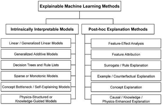
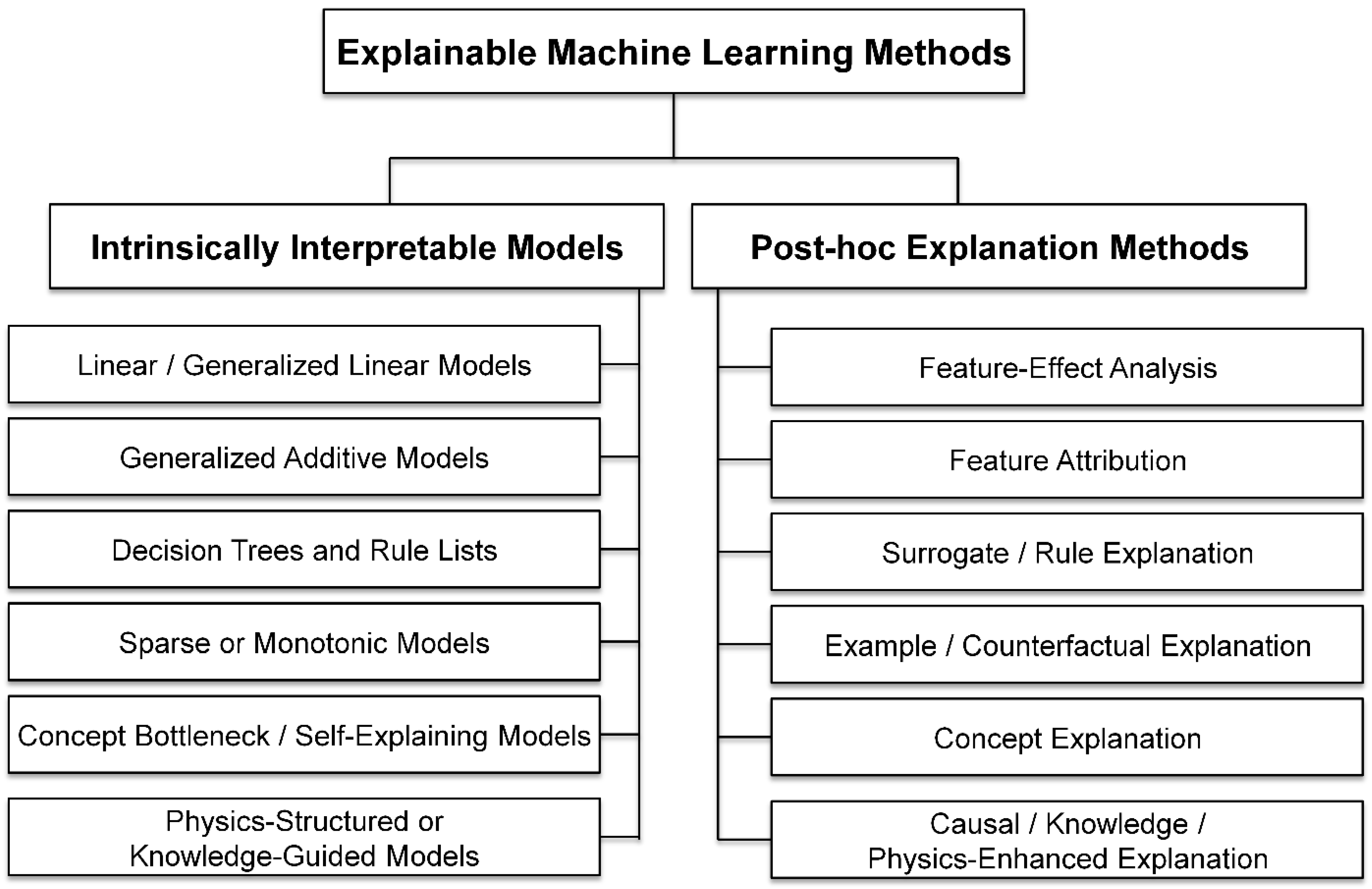
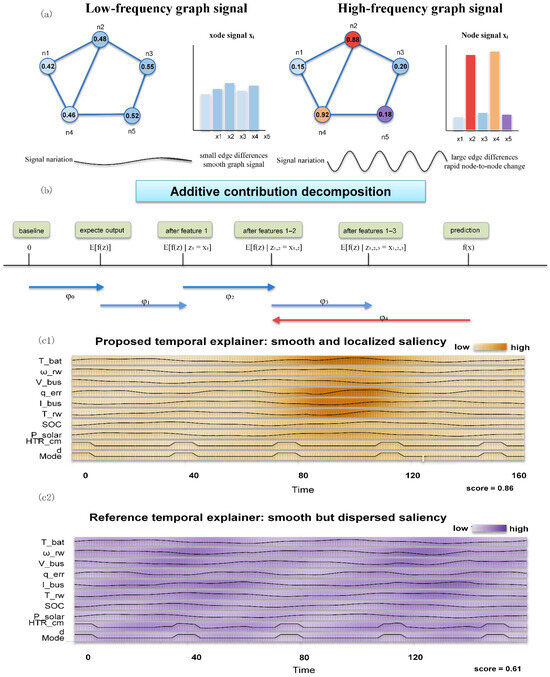
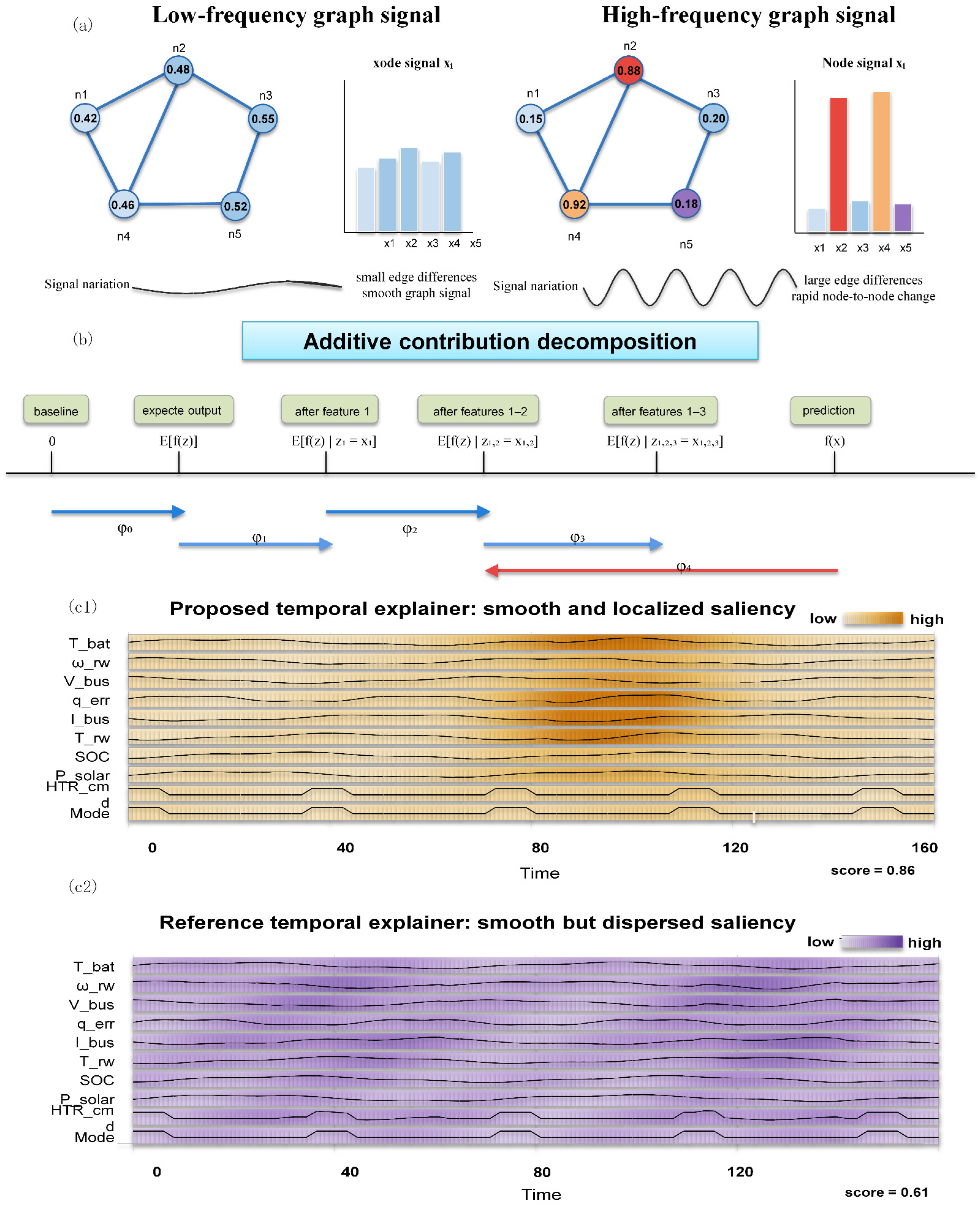
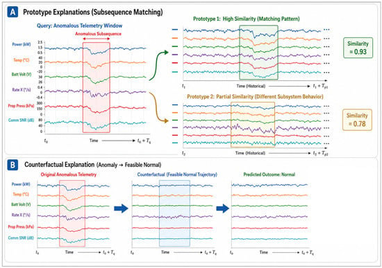
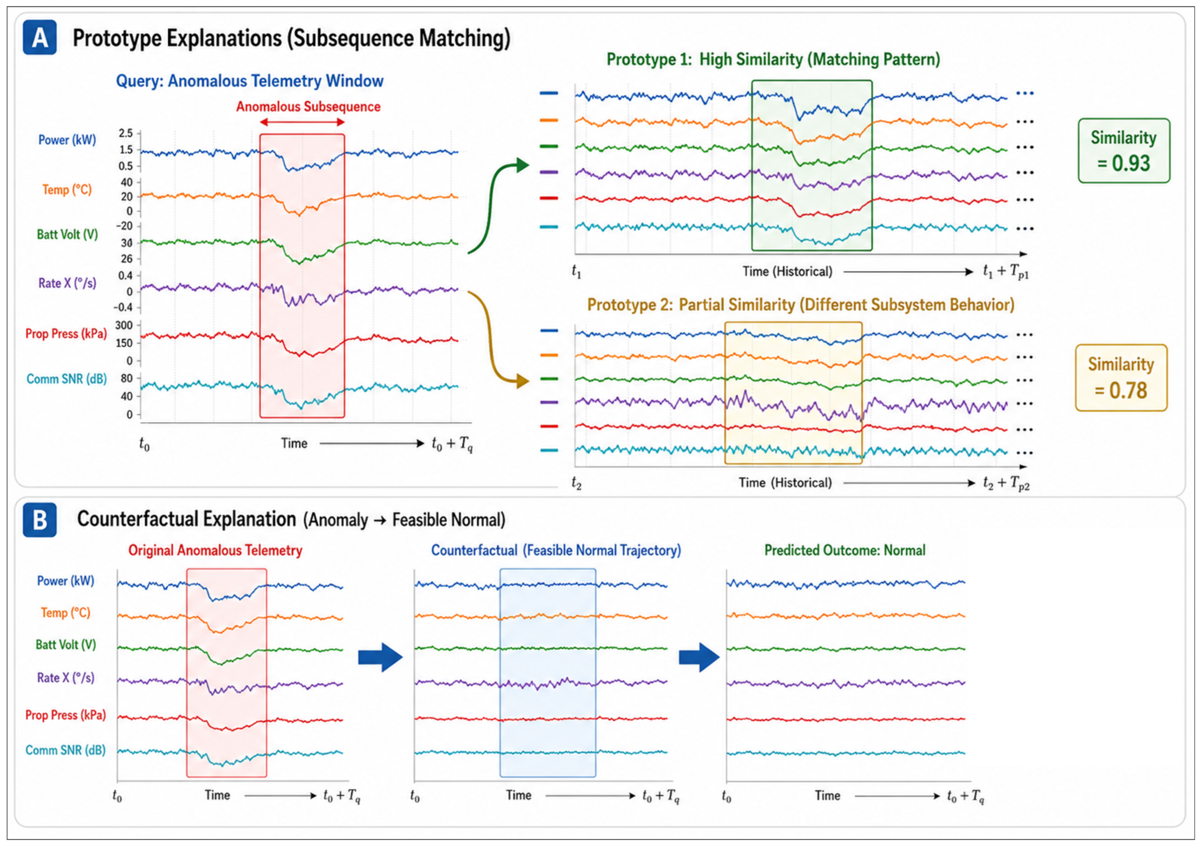
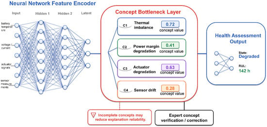
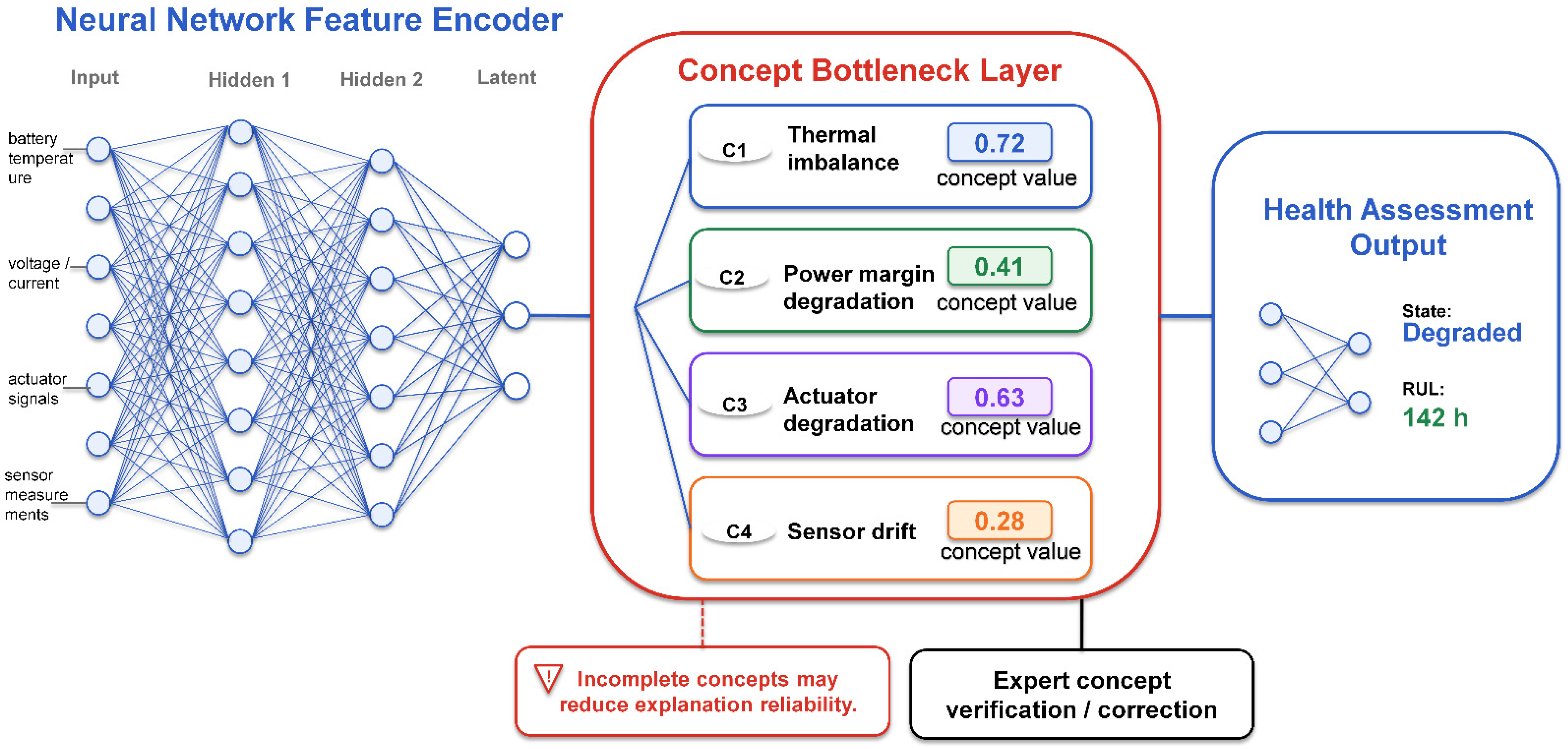
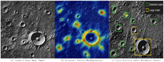
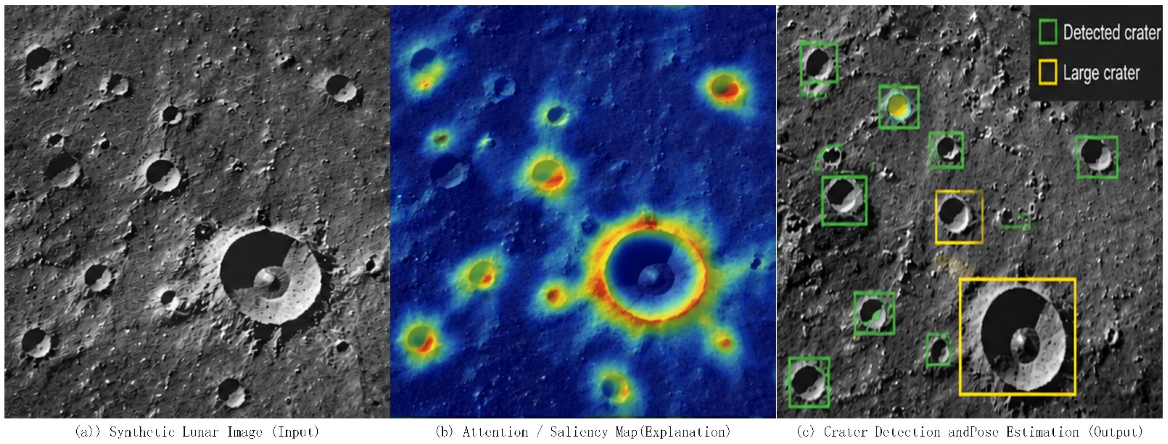
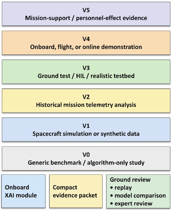
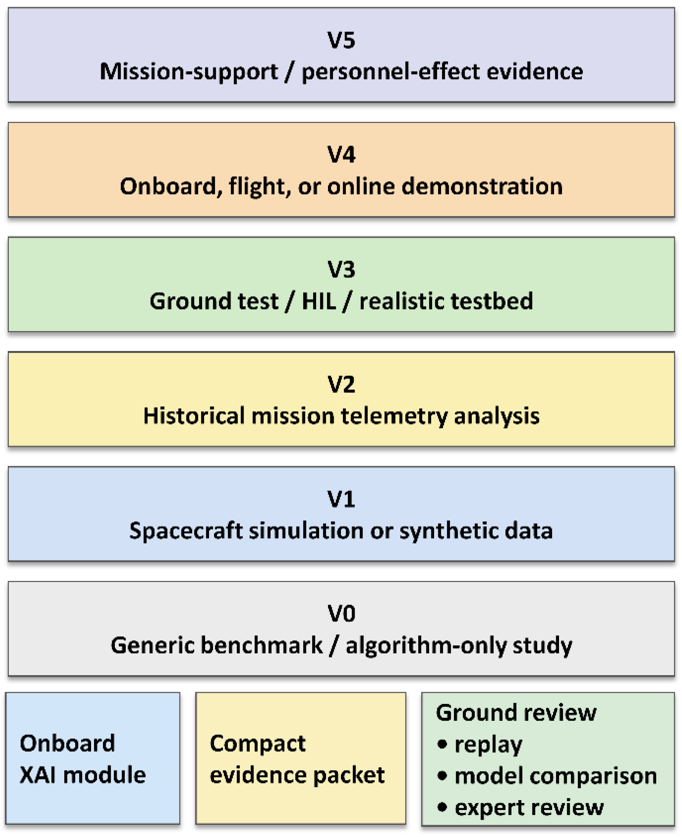

Disclaimer/Publisher’s Note: The statements, opinions and data contained in all publications are solely those of the individual author(s) and contributor(s) and not of MDPI and/or the editor(s). MDPI and/or the editor(s) disclaim responsibility for any injury to people or property resulting from any ideas, methods, instructions or products referred to in the content. |
© 2026 by the authors. Licensee MDPI, Basel, Switzerland. This article is an open access article distributed under the terms and conditions of the Creative Commons Attribution (CC BY) license.