VRGAN: A Deep Generative Framework for Unsupervised Anomaly Detection in Multivariate Time-Series Data

Abstract

Time-series anomaly detection holds value across various research fields and application domains, serving purposes such as fault diagnosis, identification of unexpected system intrusions, or signaling the onset of new disease outbreaks. To identify anomalous timepoints in a practical manner, unsupervised learning methods have been introduced. These methods leverage normality’s feature representations to reconstruct data, determining anomalies through the calculation of anomaly scores based on reconstruction errors. Still, recent approaches assume the use of a normal dataset for model training, implicitly necessitating true anomaly labels. Furthermore, the absence of guidelines for determining anomaly thresholds hinders the easy application of current detection methods in diverse research fields. In this paper, we propose VRGAN, a deep generative anomaly detection framework designed for unsupervised multivariate time-series analysis. VRGAN stands out by eliminating the need for assumptions or true label information. Through the training of variational recurrent neural network and GAN modules on a training dataset masked for anomaly candidates, VRGAN reconstructs the dataset based on learned normal data distribution and calculates anomaly scores to identify anomalies. Evaluation on seven benchmark datasets demonstrates VRGAN’s performance improvement compared with recent unsupervised anomaly detection methods. The proposed model is further tested on a time-series metagenomic dataset, showcasing its applicability in fully unsupervised settings for wastewater-based surveillance to monitor and track patterns of antibiotic resistance genes that are prevalent among bacteria carried by a given human community.

1. Introduction

Anomaly detection in time-series data has been widely studied across various domains, including fault diagnosis in machinery [1], identification of abnormal behavior in IoT sensors [2], and detection of malware or web intrusions to enhance application availability. In biological and medical research, anomalies can serve as indicators of previously unknown underlying processes, potentially critical factors in the emergence of new disease outbreaks [3,4]. It could also be used to characterize specific patients with rare or heterogeneous diseases [5]. For example, identification of temporal anomalies can potentially serve as an early warning system for antibiotic-resistant bacteria outbreaks or other events that may be relevant to antibiotic resistance stewardship and mitigation [6].

Deep learning has gained prominence in recent years for its ability to extract feature representations from complex data, making it applicable to various time-series anomaly detection methods. While some studies have employed supervised learning with labeled normal and anomalous instances for training [7,8,9], the impracticality of collecting such labeled data has led to a shift towards unsupervised approaches. Unsupervised anomaly detection involves capturing time-series embeddings or learning feature representations for data reconstruction, with anomaly scores calculated by comparing reconstructed values to actual values. Representation learning-based neural networks, including autoencoders (AEs) and deep generative models such as variational autoencoders (VAEs) and generative adversarial networks (GANs), have been adopted in recent approaches. OmniAnomaly [10] presented a stochastic recurrent neural network (RNN) combining VAEs and Gated Recurrent Units (GRUs) to explicitly model the temporal dependence and the stochasticity of time series for multivariate time-series anomaly detection in the device monitoring industry. VAE-LSTM [11] is a hybrid anomaly detection method, where the VAE module is trained to capture the low-dimensional embeddings of time-series data, while the long short-term memory-based RNN (LSTM) module takes the embeddings produced by VAE and learns the sequential patterns over extended time periods. USAD [12] proposed AEs, which were trained within an adversarial training inspired by GANs to amplify the reconstruction error of inputs containing anomalies. SISVAE [13] designed a multivariate time-series anomaly detection model based on the sequential VAE trained with a variational smoothness regularizer, providing robustness of the reconstruction by incorporating a penalty on the non-smooth output of the generative model.

State-of-the-art methods have demonstrated improved performance in time-series anomaly detection using public benchmark datasets, mostly related to server or IT system monitoring [10,11,12]. However, applying these methods to other domains, such as bioinformatics, presents numerous challenges. An assumption underlying most prior studies is that the training dataset used to identify the anomaly in the future unseen observations consists of normally distributed data points, which does not define the anomaly detection problem in the fully unsupervised setting. Moreover, a key aspect to anomaly detection is the threshold score that is used to determine whether an instance is anomalous. Often, threshold determination/selection is incorporated into model performance evaluation, where the value producing the highest performance metrics, such as the F1-score, for the validation data is set as the threshold. However, such assumptions and strategies are problematic in most biological settings. First, it is difficult to provide the human-annotated labels for biological time-series datasets. Second, if the validation set does not include any anomalous cases, the aforementioned method for determining the threshold value will not work. Third, during the performance evaluation, for some benchmark datasets, most studies adopted “point adjustment (PA) evaluation protocol”, where performance is measured based on the segment-level predictions adjusted by point predictions: if at least one point in a contiguous segment is detected as an anomaly, the entire segment is considered to be correctly predicted as an anomaly. This protocol was proposed on the basis that a single alert within an anomaly period is sufficient to take action for system recovery. However, the practice has a possibility of overestimating the model performance, as argued in several papers [14,15].

The present work proposes VRGAN, a deep generative method for time-series anomaly detection that operates in fully unsupervised settings. To mitigate the impact of anomalies on model training, potential anomalous points are identified and masked, and the remaining data is input into a variational recurrent neural network (VRNN) module. The VRNN module is trained, outputs the reconstructed points, and the learned latent variables are fed into the GAN module. After GAN module training, the anomaly threshold is defined using reconstructed values from both VRNN and GAN to predict anomalous points. VRGAN is compared with eight baseline methods on seven benchmark datasets spanning web traffic, industrial processes, spacecraft telemetry, and server monitoring and produced the best prediction performance. The experiments include comparisons under point-wise and PA evaluation protocols, component ablations, sensitivity analyses of anomaly candidate identification and decision thresholds, and an assessment of computational costs. In addition, VRGAN was applied to the time-series metagenomic datasets collected from a local wastewater treatment plant (WWTP), consisting of short-read relative abundance values of antibiotic resistance genes (ARGs). Predicted anomalous points were validated through several analyses. VRGAN is publicly accessible at https://github.com/joungmin-choi/VRGAN (accessed on 1 September 2026).

2. Materials and Methods

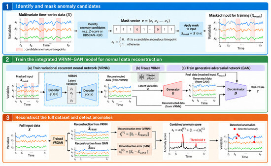
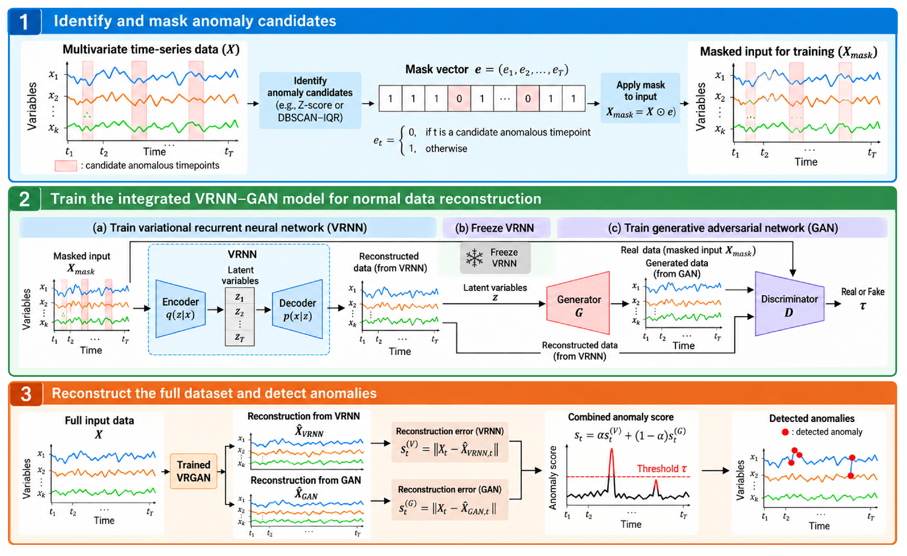
This section describes the system of VRGAN, illustrated in Figure 1. Our model consists of three phases. Initially, we identify a set of anomaly candidates and mask those points during training to prevent the model from being influenced by anomalies. Subsequently, the VRNN is trained to learn the latent variables, capturing temporal dependencies among variables across timesteps and reconstructing the input. The learned latent variables are then fed into the GAN module, which is trained to reconstruct the input as well. Utilizing the reconstructed values from both the VRNN and GAN modules, an anomaly detection threshold is determined. Samples with anomaly scores surpassing this threshold are predicted as anomalous.

Figure 1. Workflow of the proposed anomaly identification framework.

2.1. Defining the Mask Based on the Anomaly Candidates

Let n be the number of features, $T=(t_1$, $t_2$, …, $t_k)$ a positive increasing sequence of times, $x_i\in {\mathbf{R}}^n$ the observations at time $t_i$, and $x=(x_1$, …, $x_k)\in {\mathbf{R}}^{n\times k}$ the matrix of all the $x_i$. To minimize the influence of anomalies on model training, a set of candidate anomalous timepoints are identified and masked before training, where the mask vector $e\in {\{0,1\}}^k$ is defined by

$$\begin{array}{c}\hfill e_i=\left\{\begin{array}{cc}0,\hfill & \mathrm{if}{t}_i\mathrm{is}\mathrm{a}\mathrm{candidate}\mathrm{anomalous}\mathrm{timepoint},\hfill \\ 1,\hfill & \mathrm{otherwise}.\hfill \end{array}\right.\end{array}$$

(1)

When true anomaly labels are available for the training set, anomaly candidates can be defined based on them. However, in most cases, obtaining true labels is unrealistic. Two approaches can be employed to identify anomaly candidates. The first approach utilizes the standard deviation information from the dataset, calculating the Z-Score for each feature. If a timepoint has at least $1\%$ of the number of highly variant features (defined as |Z-Score| > 2), the timepoint is considered an anomaly candidate and is masked during training. Alternatively, outliers detected by both DBSCAN and IQR rules can be used to identify candidates. Given that DBSCAN is sensitive to parameter settings [16], we consider outliers detected by both methods as candidates for anomalous timepoints and mask them. The performance of anomaly detection based on each method is presented in the Section 3.

The masking ratio is not predefined as a fixed proportion of the time series but is adaptively determined by the identified anomaly candidates. Specifically, the masking ratio is defined as the number of masked timepoints divided by the total number of timepoints. For the Z-score-based strategy, the criterion requiring at least 1% highly variant features refers to the proportion of features used to identify an anomaly candidate, rather than the proportion of timepoints to be masked. For the combined DBSCAN–IQR strategy, only timepoints identified as outliers by both methods are selected as anomaly candidates. Consequently, the masking ratio depends on the statistical characteristics of the dataset and the hyperparameters of the selected candidate identification strategy, without requiring ground-truth anomaly labels.

2.2. Data Reconstruction Based on VRGAN

2.2.1. Phase 1: VRNN Module Training

The variational recurrent neural network (VRNN) [17] extends the variational autoencoder (VAE) into a recurrent framework for modeling high-dimensional sequences. VAE, a probabilistic generative model combining a neural network and a variational learning framework, introduces latent variables z to capture variations in observed variables x. The VAE models the conditional $p\left(x\right|z)$ with a neural network, assuming a standard normal distribution for the prior over latent variables $p\left(z\right)$. However, introducing a non-linear mapping from z to x leads to intractable inference of the posterior $p\left(z\right|x)$. To resolve this, VAE employs variational inference, approximating the posterior as a Gaussian. Through stochastic gradient variational Bayes, VAE estimates Gaussian parameters $\mu$ and $\sigma$, using the variational lower bound on the log-likelihood as the objective function:

$$\begin{array}{c}\hfill \log p\left(x\right)\ge E_{q\left(z\right|x)}\left[\log p\left(x\right|z)\right]-KL\left(q\left(z\right|x)\right|\left|p\left(z\right)\right),\end{array}$$

(2)

where $KL\left(Q\right|\left|P\right)$ denotes the Kullback-Leibler (KL) divergence between probability distributions Q and P. The encoder, termed the inference model $q\left(z\right|x)$, and the decoder, defining the generative model $p\left(x\right|z)$, are trained jointly by maximizing the variational lower bound.

The VRNN incorporates a VAE at each timestep, with VAEs conditioned on the RNN’s hidden state variable $h_{i-1}$ to consider the temporal structure of sequential data. It integrates temporal dependency modeling with probabilistic latent variable learning, both of which are essential to the objectives of the proposed VRGAN framework. Unlike conventional deterministic recurrent encoders, the VRNN incorporates variational inference at each timepoint, enabling the learning of stochastic latent representations conditioned on preceding temporal information. This probabilistic formulation jointly models temporal dependencies and variability in the observed time-series data. Furthermore, the learned latent representations can be transferred to the subsequent GAN module to produce complementary reconstructions. The VRNN is also augmented with adaptive smoothness regularization, which encourages temporal consistency while reducing the regularization strength for observations exhibiting larger statistical deviations. Therefore, the VRNN was adopted for its compatibility with probabilistic reconstruction, temporal modeling, and the sequential training strategy of VRGAN, rather than based on an assumption that recurrent architectures are inherently superior to alternative temporal encoders.

The prior on the latent variable follows the distribution:

$$\begin{array}{c}\hfill z_i\sim N({\mu }_{0,i},\mathrm{diag}\left({\sigma }_{0,i}^2\right)),\mathrm{where}[{\mu }_{0,i},{\sigma }_{0,i}]={\phi }_{\theta }^{\mathrm{prior}}\left(h_{i-1}\right),\end{array}$$

(3)

where ${\mu }_{0,i}$ and ${\sigma }_{0,i}$ denotes to the parameters of the conditional prior distribution. The generating distribution will also be conditioned on $h_{i-1}$ and $z_i$:

$$\begin{array}{c}\hfill x_i|z_i\sim N({\mu }_{x,i},\mathrm{diag}\left({\sigma }_{x,i}^2\right)),\mathrm{where}[{\mu }_{x,i},{\sigma }_{x,i}]={\phi }_{\theta }^{\mathrm{dec}}({\phi }_{\theta }^z\left(z_i\right),h_{i-1}),\end{array}$$

(4)

with ${\mu }_{x,i}$ and ${\sigma }_{x,i}$ as parameters of the generating distribution, ${\phi }_{\theta }^{\mathrm{prior}}$ and ${\phi }_{\theta }^{\mathrm{dec}}$ representing neural networks. Additionally, ${\phi }_{\theta }^x$ and ${\phi }_{\theta }^z$ refers to neural networks extracting features from $x_i$ and $z_i$, respectively. The RNN updates its hidden state using the recurrence equation:

$$\begin{array}{c}\hfill h_i=f({\phi }_{\theta }^x\left(x_i\right),{\phi }_{\theta }^z\left(z_i\right),h_{i-1}),\end{array}$$

(5)

where f is a non-linear transition function. The generative model results in the following factorization:

$$\begin{array}{c}\hfill p(x_{\le k},z_{\le k})={\displaystyle \prod _{i=1}^k}p\left(x_i\right|z_{\le i},x_{<i})p\left(z_i\right|x_{<i},z_{<i})\end{array}$$

(6)

In a similar fashion, the approximate posterior depends on $x_i$ and $h_{i-1}$:

$$\begin{array}{c}\hfill z_i|x_i\sim N({\mu }_{z,i},\mathrm{diag}\left({\sigma }_{z,i}^2\right)),\mathrm{where}[{\mu }_{z,i},{\sigma }_{z,i}]={\phi }_{\varphi }^{\mathrm{enc}}({\phi }_{\theta }^x\left(x_i\right),h_{i-1}),\end{array}$$

with ${\mu }_{z,i}$ and ${\sigma }_{z,i}$ as parameters of the approximate posterior, and ${\phi }_{\varphi }^{\mathrm{enc}}$ approximated by a neural network. The encoder for the approximate posterior and the decoder for the generative model are tied through the RNN hidden state $h_{i-1}$. The inference model results in the following factorization:

$$\begin{array}{c}\hfill q\left(z_{\le k}\right|x_{\le k})={\displaystyle \prod _{i=1}^k}q\left(z_i\right|x_{\le i},z_{<i}).\end{array}$$

(7)

The objective function of VRNN becomes a timestep-wise variational lower bound:

$$\begin{array}{c}\hfill {\displaystyle \sum _{i=1}^k}\{\log p\left(x_i\right|z_{\le i},x_{<i})-\mathrm{KL}(q\left(z_i\right|x_{\le i},z_{<i})\left|\right|p\left(z_i\right|x_{<i},z_{<i})\left)\right\}\end{array}$$

(8)

In addition, the smoothness regularization was added, following the idea suggested by Li et al. [13]. Assuming that the probability density function over time varies smoothly, the cumulative transition cost of time-varying probability distributions is defined as follows:

$$\begin{array}{c}\hfill L_{\mathrm{smooth}}={\displaystyle \sum _{i=1}^{k-1}}{\lambda }_i\mathrm{KL}\left(p\left(x_i\right|z_{\le i},x_{<i})\parallel p\left(x_{i+1}\right|z_{\le i+1},x_{<i+1})\right).\end{array}$$

(9)

Here, ${\lambda }_i$ denotes the smoothness regularization coefficient associated with timepoint $t_i$. For the Z-score-based anomaly candidate identification strategy, this coefficient is dynamically determined based on the statistical deviation of each observation. Specifically, the Z-score of feature j at timepoint $t_i$ is calculated as follows:

$$\begin{array}{c}\hfill z_{i,j}={\displaystyle \frac{x_{i,j}-{\mu }_j}{{\sigma }_j+ϵ}},\end{array}$$

(10)

where $x_{i,j}$ represents the observed value of feature j at timepoint $t_i$, ${\mu }_j$ and ${\sigma }_j$ denote the mean and standard deviation of feature j calculated from the training time series, respectively, and $ϵ={10}^{-8}$ is a small positive constant introduced for numerical stability. The absolute Z-scores are then averaged across all n features to obtain a timepoint-level anomaly magnitude:

$$\begin{array}{c}\hfill a_i={\displaystyle \frac{1}{n}}{\displaystyle \sum _{j=1}^n}\left|z_{i,j}\right|.\end{array}$$

(11)

The resulting anomaly magnitude is normalized by the maximum value across the training time series, and the time-dependent smoothness regularization coefficient is defined as follows:

$$\begin{array}{c}\hfill {\lambda }_i=1-{\displaystyle \frac{a_i}{{\max }_{1\le t\le k}{a}_t+ϵ}}.\end{array}$$

(12)

Accordingly, ${\lambda }_i\in [0,1]$, with larger mean absolute Z-scores resulting in smaller regularization coefficients. This adaptive weighting reduces the smoothness constraint on potentially anomalous timepoints while assigning larger coefficients to observations exhibiting smaller statistical deviations. The coefficient ${\lambda }_i$ is applied to the KL divergence between the reconstructed probability distributions at consecutive timepoints $t_i$ and $t_{i+1}$. For the combined DBSCAN–IQR anomaly candidate identification strategy, the coefficient is fixed at ${\lambda }_i=0.5$ during training. The coefficient is also initialized to 0.5 for the testing dataset, although smoothness regularization is applied only during model training.

The final objective function for training the VRNN is therefore expressed as:

$$\begin{array}{cc}\hfill L_{\mathrm{VRNN}}=& -{\displaystyle \sum _{i=1}^k}\left\{\log p\left(x_i\right|z_{\le i},x_{<i})-\mathrm{KL}\left(q\left(z_i\right|x_{\le i},z_{<i})\parallel p\left(z_i\right|x_{<i},z_{<i})\right)\right\}\hfill \\ & +{\displaystyle \sum _{i=1}^{k-1}}{\lambda }_i\mathrm{KL}\left(p\left(x_i\right|z_{\le i},x_{<i})\parallel p\left(x_{i+1}\right|z_{\le i+1},x_{<i+1})\right).\hfill \end{array}$$

(13)

As a final output, the VRNN will produce the reconstructed dataset $\hat{x}$.

2.2.2. Phase 2: GAN Module Training

After training the VRNN, the learned latent variables from the VRNN were transferred to the generator in the GAN module as an input, with latent variables for timepoints in the anomaly candidates being masked. To train temporal relations between the observations, a one-layer RNN module was implemented, followed by a fully connected layer. From this module, the generated output $\overline{x}$ was obtained and multiplied by a combination factor $\gamma$ to calculate the final reconstructed output: $\tilde{x}=\gamma \overline{x}$.

The combination factor is based on the time gap $\delta \in {\mathbf{R}}^k$ and is trained as a model parameter controlling the influence of the forward-generated values based on how far the last observed value in the forward direction was:

$$\begin{array}{cc}\hfill \gamma & =\exp \left(-\max \{0,f_{\gamma }\left(\delta \right)\}\right),\hfill \end{array}$$

(14)

where $f_{\gamma }$ is a fully connected layer with a ReLU activation function, and the time gap is defined as the time lag between the current and previous values in the forward direction, given by:

$$\begin{array}{c}\hfill {\delta }_i=\left\{\begin{array}{cc}{t}_i-t_{i-1},\hfill & \mathrm{if}{e}_{i-1}=1,i>1,\hfill \\ {\delta }_{i-1}+t_i-t_{i-1},\hfill & \mathrm{if}{e}_{i-1}=0,i>1,\hfill \\ 0,\hfill & \mathrm{if}i=1.\hfill \end{array}\right.\end{array}$$

(15)

During the training phase, the generator was trained to minimize the loss composed of two different losses, expressed as follows:

$$\begin{array}{c}\hfill L_{\mathrm{Gen}}=L_G+L_R.\end{array}$$

(16)

$L_G$ represents the classification loss, where the generator aims to maximize the probability $D\left(\tilde{x}\right)$ that the discriminator D (defined later) classifies the fake instances as actual values:

$$\begin{array}{c}\hfill L_G=-\log \left(D\left(\tilde{x}\right)\right).\end{array}$$

(17)

To train the generator such that its outputs are close to the corresponding actual values in the input, the reconstruction loss $L_R$ is defined as the absolute error between the actual values and the corresponding generated values:

$$\begin{array}{c}\hfill L_R={\displaystyle \sum _{i=1}^k}{∥(x_i-{\tilde{x}}_i)e_i∥}_1/{\parallel e\parallel }_1.\end{array}$$

(18)

The discriminator takes the two reconstructed values $\hat{x}$ and $\tilde{x}$ from the VRNN and the generator module, respectively, along with the actual observation values x as input. It consists of a one-layer RNN module followed by two fully connected layers and a sigmoid function, classifying the input as real or generated values. The discriminator is trained to maximize the probability of correctly classifying actual values as real and generated values as fake using a binary cross-entropy loss:

$$\begin{array}{c}\hfill L_{\mathrm{Disc}}=-\log \left(D(x\odot e)\right)-\log (1-D\left(\tilde{x}\right))-\log (1-D\left(\hat{x}\right)),\end{array}$$

(19)

where $D(x\odot e)$ is the probability for the actual value to be classified as real, $1-D\left(\tilde{x}(\mathrm{or}\hat{x}\right))$ is the probability of the reconstructed value being classified as fake. While training the GAN module, the VRNN module is frozen to avoid its impact on the GAN module training.

2.3. Calculation of the Anomaly Score and the Threshold

To identify anomalous observations, VRGAN calculates the anomaly score by combining the reconstruction errors obtained from the VRNN and GAN modules. The anomaly score $s_i$ for observation $x_i$ is defined as follows:

$$s_i=\underset{s_i^{\mathrm{VRNN}}}{\underbrace{\parallel x_i-{\hat{x}}_i{\parallel }_2}}+\underset{s_i^{\mathrm{GAN}}}{\underbrace{\parallel x_i-{\tilde{x}}_i{\parallel }_2}},$$

(20)

where ${\parallel ·\parallel }_2$ denotes the Euclidean norm, and $s_i^{\mathrm{VRNN}}$ and $s_i^{\mathrm{GAN}}$ represent the reconstruction errors from the VRNN and GAN modules, respectively. The two errors are calculated in the same observation space and combined with equal weights. A larger score indicates greater disagreement between the original observation and the reconstructed outputs.

The anomaly detection threshold is determined using the validation set without requiring ground-truth anomaly labels. Let $\mathcal{V}$ denote the set of validation timepoint indices. Using the masking indicator $e_i$ defined in Equation (1), the threshold $\alpha$ is calculated as follows:

$$\alpha =\underset{\begin{array}{c}i\in \mathcal{V}\\ e_i=1\end{array}}{\max }{s}_i.$$

(21)

An observation is classified as anomalous when $s_i>\alpha$ and as normal otherwise.

Unlike conventional VAE-based reconstruction methods that primarily rely on a single generative model, VRGAN employs a two-stage architecture integrating variational recurrent modeling and adversarial generation. The VRNN first learns temporal dependencies and latent representations, which are subsequently transferred to the GAN module. During the second training stage, the VRNN parameters are frozen, allowing the GAN to learn an additional reconstruction without modifying the pretrained VRNN. Unlike approaches that rely on reconstruction errors from a single model, VRGAN combines the reconstruction errors of both modules to calculate anomaly scores. In addition, anomaly candidate masking is applied during training to mitigate the influence of potentially anomalous observations, and the detection threshold is determined from validation data without using ground-truth anomaly labels. These design choices distinguish VRGAN from standalone VAE-, GAN-, and recurrent reconstruction-based frameworks in terms of model integration, training procedure, and anomaly-scoring strategy.

2.4. Implementation of the VRGAN

The VRNN module comprises a single current hidden layer with 8 GRU units, and ${\phi }^x$, ${\phi }^z$, ${\phi }^{\mathrm{prior}}$ include two fully connected (FC) layers using rectified linear units (ReLU) with 8 hidden nodes. Notably, ${\phi }^{\mathrm{prior}}$ employs the Softplus function for the last layer. On the other hand, ${\phi }^{\mathrm{enc}}$ consists of two FC layers with 32 and 16 hidden nodes, followed by a ReLU activation function. The symmetrical structure of ${\phi }^{\mathrm{dec}}$ mirrors ${\phi }^{\mathrm{enc}}$, extracting 8 latent variables with a sigmoid function. For the GAN module, the generator features a single recurrent hidden layer with 16 GRU units followed by an FC layer with a sigmoid function. The discriminator is constructed with a one-layer RNN having 16 LSTM units, followed by two FC layers ending with the sigmoid function.

VRGAN was trained with Adam, an adaptive optimization algorithm [18], with a learning rate of ${10}^{-4}$. The VRNN module underwent initial training for 1000 epochs. Subsequently, the GAN module was trained for an additional 1000 epochs, with the VRNN being frozen during GAN training. For each epoch, the generator was trained after five iterations of the discriminator.

2.5. Experimental Design

To assess the performance of our proposed model, seven publicly available benchmark datasets were employed. Table 1 provides an overview of the dataset characteristics. The Yahoo’s S5 Webscope A1 dataset (Yahoo-A1) [19] consists of 67 univariate time-series data collected from computation systems, recording real production traffic of Yahoo’s Website, with anomalies annotated manually by human experts.

Table 1. Details of the benchmark datasets used for performance evaluation.

Dataset	Description	Number of Time-Series	Number of Features	Length	Proportion of Anomalies	Anomaly Label
Yahoo-A1	Real production traffic of Yahoo’s Website dataset	67	1	1420	1.58%	Train, Validation, Test
SKAB-valve1	Skoltech anomaly benchmark valve1 dataset	1	8	18,160	34.74%	Train, Validation, Test
SKAB-valve2	Skoltech anomaly benchmark valve2 dataset	1	8	4310	35.19%	Train, Validation, Test
TEP	Tennessee Eastman Process	60	52	1460	50%	Train, Validation, Test
SMAP	Soil Moisture Active Passive satellite dataset	55	25	11,000	13.13%	Test
MSL	Mars Science Laboratory rover dataset	27	55	4000	10.72%	Test
SMD	Server Machine Dataset	28	38	50,000	4.16%	Test
CIWARS	Metagenomic sequencing data from a WWTP	1	15	80	Unknown	-

SKAB [20] is the Skoltech anomaly benchmark dataset designed for evaluating anomaly detection algorithms. Each dataset, representing valve1 and valve2, respectively, consists of 8 variables. True labels for single-point anomalies were provided by human experts.

The Tennessee Eastman Process (TEP) dataset [21] is a simulated industrial process dataset widely used for fault detection and diagnosis. It contains 52 process variables, comprising 41 continuous process measurements and 11 manipulated variables. For computational efficiency, we selected 30 independent simulation runs for each of two operating conditions: normal operation (fault number 0) and fault condition 1, resulting in 60 time series. Each time series contained 500 training samples and 960 testing samples, with ground-truth anomaly labels available for both partitions.

Soil Moisture Active Passive (SMAP) satellite and Mars Science Laboratory (MSL) rover datasets are expert-labeled datasets from NASA [22], each comprising 55 and 27 time-series data composed of 25 and 55 variables, respectively. The Server Machine Dataset (SMD) is a 5-week-long dataset collected from a large internet company, which consists of 28 different machines, as provided by [10].

To test the robustness of the methods in anomaly detection across different research domains, our proposed model and other baseline methods were compared using a time-series metagenomic dataset from the NSF-funded CyberInfrastructure for Waterborne Antibiotic Resistance Risk Surveillance (CIWARS) project (PRJNA1083020) [23]. Collected from sampling influent wastewater to the wastewater treatment plant (WWTP) in a local WWTP from August 2020 to July 2021, the dataset includes short-read abundance values for antibiotic resistance genes (ARGs) measured by DeepARG [24]. After preprocessing, 221 common ARGs shown in all the timepoints were selected, and the 16S normalized abundances of ARGs were aggregated for each drug resistance class, resulting in 15 classes. Metadata for the influent, primary, aeration tank, effluent water quality parameters, and the rainfall during sampling were collected. Descriptions for each parameter is provided in Supplementary Material S5.

For performance evaluation, the Yahoo-A1 and SKAB datasets were split to a ratio of 3:2:5 for training, validation and testing. Models were trained on the training dataset, and the anomaly threshold was defined based on the validation set. For TEP, SMAP, MSL, and SMD datasets, pre-defined training and testing datasets were available, with anomaly label information provided solely for the testing dataset. The training dataset was split into a 3:2 ratio for training and validation sets. All the datasets were normalized using min-max normalization. In each experiment, the average Area Under the Receiver Operating Characteristic Curve (AUROC) and the F1-score were measured for the testing dataset, utilizing the Scikit-learn package [25].

3. Results

3.1. Performance Evaluation of VRGAN

To demonstrate the effectiveness and generalizability of our proposed VRGAN model across different scenarios, we conducted a comprehensive performance evaluation using real-world benchmark datasets. First, the models were evaluated on four datasets with ground-truth anomaly labels available for the entire dataset, including the training, validation, and testing sets: Yahoo-A1, SKAB-valve1, SKAB-valve2, and TEP. The performance of VRGAN was assessed under three conditions: (1) using ground-truth anomaly labels, (2) employing outliers detected by both DBSCAN and IQR, and (3) utilizing standard deviation information. These conditions were denoted as ‘VRGAN (true)’, ‘VRGAN (outlier)’, and ‘VRGAN (SD)’, respectively. To provide a comprehensive comparison across different deep learning architectures, VRGAN was evaluated against eight baseline methods, including Anomaly-Transformer, a Transformer-based anomaly detection model; MADGAN, a GAN-based anomaly detection model; SISVAE, a sequential variational autoencoder with smoothness regularization; VAE-LSTM, which combines variational autoencoders and long short-term memory networks; USAD, an adversarially trained autoencoder-based method; and three recurrent generative models, VRNN-GRU, VAE-RNN, and GAN-RNN. The baseline methods utilized ground-truth labels from the validation set to determine the anomaly detection threshold, selecting the threshold that maximized the F1-score. Each experiment was repeated five times, and the mean performance results are presented in Table 2 and Figure 2, with the corresponding standard deviations reported in Supplementary Material S1. One-sided Wilcoxon signed-rank tests were performed for F1-scores to assess the statistical significance of performance differences.

Table 2. Average anomaly detection performance on four benchmark datasets with ground-truth anomaly labels available for the training and validation sets. Results represent the mean performance over five independent runs, with the corresponding standard deviations reported in Supplementary Material S1. One-sided Wilcoxon signed-rank tests were performed on the F1-scores to assess statistical significance. An asterisk (*) indicates a statistically significant improvement of the best-performing VRGAN variant over the corresponding comparison method (p < 0.05); non-significant comparisons are left unmarked.

Dataset	Metric	VRGAN (True)	VRGAN (Outlier)	VRGAN (SD)	Anomaly-Transformer	MADGAN	SISVAE	VAE-LSTM	USAD	VRNN-GRU	VAE-RNN	GAN-RNN
Yahoo-A1	Precision	0.303	0.320	0.288	0.085	0.091	0.212	0.180	0.054	0.215	0.216	0.186
	Recall	0.420	0.360	0.676	0.023	0.209	0.354	0.320	0.504	0.358	0.380	0.248
	F1-score	0.289	0.270	0.295	0.015 *	0.073 *	0.209	0.184 *	0.085 *	0.212	0.221	0.147 *
SKAB-valve1	Precision	0.983	0.949	0.937	0.557	0.359	0.345	0.343	0.995	0.345	0.343	0.343
	Recall	0.437	0.445	0.441	0.081	0.944	0.996	1.000	0.374	0.996	1.000	1.000
	F1-score	0.567	0.606	0.595	0.140 *	0.518	0.513	0.511	0.544	0.513	0.511	0.511
SKAB-valve2	Precision	0.980	0.959	0.944	0.358	0.456	0.465	0.412	0.764	0.412	0.412	0.412
	Recall	0.409	0.357	0.357	0.036	0.907	0.300	0.600	0.358	0.600	0.600	0.600
	F1-score	0.553	0.520	0.516	0.065 *	0.607	0.365 *	0.489	0.488	0.489	0.489	0.489
TEP	Precision	0.500	0.500	0.500	0.437	0.500	0.500	0.500	0.500	0.500	0.500	0.500
	Recall	0.059	0.186	0.149	0.003	0.106	0.092	0.093	0.173	0.173	0.173	0.078
	F1-score	0.103	0.270	0.225	0.005 *	0.159	0.152 *	0.153 *	0.257	0.257	0.257	0.135 *

Note: Bold values indicate the highest F1-score among the VRGAN variants for each dataset.

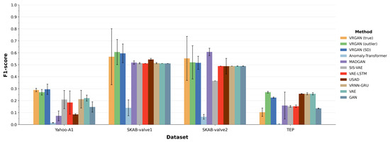
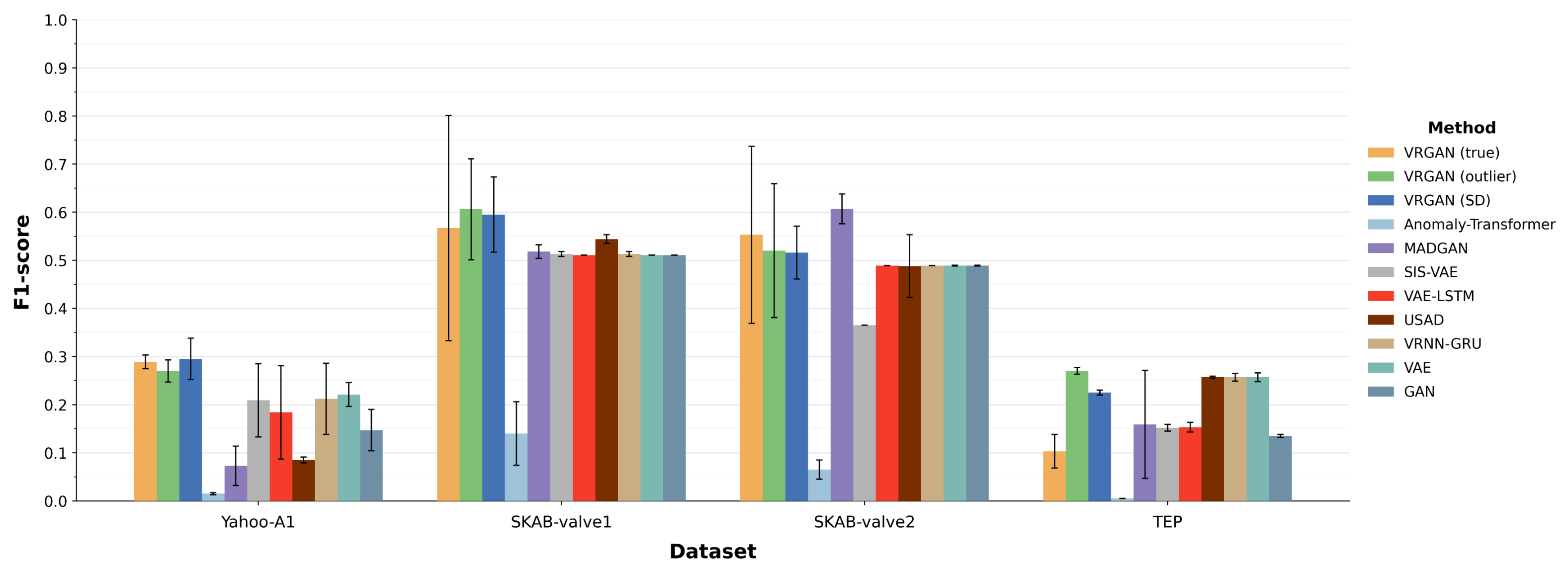
Figure 2. Performance comparison of VRGAN models with the baseline methods based on the datasets having the true anomaly labels.

As shown in Table 2 and Figure 2, VRGAN achieved the highest F1-scores among the evaluated methods on three of the four datasets, including Yahoo-A1, SKAB-valve1, and TEP. On Yahoo-A1, VRGAN (SD) achieved the highest F1-score of 0.295, outperforming all baseline methods, including VAE-RNN (0.221), VRNN-GRU (0.212), SISVAE (0.209), and VAE-LSTM (0.184). Similarly, on SKAB-valve1, VRGAN (outlier) achieved the highest F1-score of 0.606, exceeding the results of USAD (0.544), MADGAN (0.518), and the recurrent generative models (0.511–0.513). On the TEP dataset, VRGAN (outlier) achieved the highest F1-score of 0.270, followed by USAD, VRNN-GRU, and VAE-RNN (0.257). In contrast, on SKAB-valve2, MADGAN achieved the highest F1-score of 0.607, followed by VRGAN (true) (0.553), while VRGAN (outlier) and VRGAN (SD) achieved 0.520 and 0.516, respectively. These results demonstrate the competitive performance of VRGAN against Transformer-based, GAN-based, and recurrent generative models across different datasets, although its relative performance varies depending on the dataset characteristics.

Notably, VRGAN using statistically identified anomaly candidates achieved higher F1-scores than its counterpart using ground-truth anomaly labels on three of the four datasets. Specifically, VRGAN (SD) achieved F1-scores of 0.295 and 0.595 on Yahoo-A1 and SKAB-valve1, respectively, exceeding the corresponding results obtained using ground-truth anomaly labels (0.289 and 0.567). Similarly, on TEP, VRGAN (outlier) achieved an F1-score of 0.270, compared with 0.103 for VRGAN (true). Although VRGAN (true) achieved a higher F1-score on SKAB-valve2 (0.553) than its label-free variants (0.516), these findings suggest that statistically identified anomaly candidates can serve as an effective alternative to ground-truth labels and, in certain datasets, improve anomaly detection performance. Importantly, these results highlight the distinguishing contribution of VRGAN. Rather than assuming that the training data contain only normal observations or requiring ground-truth anomaly labels to identify contaminated samples, VRGAN identifies potential anomalies using statistical characteristics of the observed data and masks these candidates during model training. This strategy is integrated with a two-stage generative framework in which the VRNN captures temporal dependencies and latent representations, while the GAN module provides complementary reconstruction estimates. The reconstructed outputs from both modules are combined to calculate anomaly scores, and the detection threshold is determined using validation data without requiring ground-truth labels. The consistent improvements over several baseline methods on Yahoo-A1, SKAB-valve1, and TEP, together with the effectiveness of label-free anomaly candidate selection, support the applicability of VRGAN across different anomaly detection settings.

Furthermore, the methods were evaluated using the SMAP, MSL, and SMD datasets, which lack ground-truth anomaly labels for the training and validation sets. Following the original studies of the comparison methods, the assumption that the training and validation datasets contain only normal timepoints was applied to the baseline methods. For these benchmark datasets, most previous studies adopted the point adjustment (PA) evaluation protocol, which assumes that a single alert within an anomalous period is sufficient for system recovery. However, this protocol has the potential to overestimate anomaly detection performance [14,15]. To provide a more comprehensive evaluation, we compared VRGAN with eight baseline methods under both evaluation protocols, with and without PA. The results are presented in Table 3, with the corresponding standard deviations provided in Supplementary Material S2. VRGAN achieved the highest F1-scores across all three datasets under both evaluation protocols. Without PA, VRGAN achieved F1-scores of 0.275, 0.307, and 0.281 on SMAP, MSL, and SMD, respectively, exceeding those of the highest-performing baseline methods, VAE-LSTM (0.247) on SMAP and USAD on MSL (0.303) and SMD (0.236). Under the PA protocol, VRGAN (SD) achieved F1-scores of 0.593, 0.580, and 0.509 on SMAP, MSL, and SMD, respectively, outperforming all eight baseline methods. These results demonstrate that VRGAN consistently achieved the highest F1-scores among the evaluated methods under both protocols, including comparisons with Transformer-based, GAN-based, and recurrent generative models. Additionally, the F1-scores increased substantially under the PA protocol, highlighting its potential to overestimate anomaly detection performance and the importance of reporting results under both evaluation settings.

Table 3. Anomaly detection performance comparison using SMAP, MSL, and SMD datasets with and without point adjustment (PA) evaluation protocol. Results represent the mean performance over five independent runs, with the corresponding standard deviations reported in Supplementary Material S2. One-sided Wilcoxon signed-rank tests were performed on the F1-scores to assess statistical significance. An asterisk (*) indicates a statistically significant improvement of the best-performing VRGAN variant over the corresponding comparison method (p < 0.05); non-significant comparisons are left unmarked.

EvaluationProtocol	Dataset	Metric	VRGAN (Outlier)	VRGAN (SD)	Anomaly-Transformer	MADGAN	SISVAE	VAE-LSTM	USAD	VRNN-GRU	VAE-RNN	GAN-RNN
w/o PA	SMAP	Precision	0.185	0.255	0.127	0.123	0.225	0.232	0.125	0.225	0.189	0.154
		Recall	0.256	0.298	0.129	0.142	0.270	0.263	0.175	0.269	0.246	0.206
		F1-score	0.215	0.275	0.128 *	0.132 *	0.245	0.247	0.146 *	0.245	0.214	0.176 *
	MSL	Precision	0.235	0.170	0.119	0.116	0.139	0.179	0.255	0.143	0.185	0.117
		Recall	0.441	0.358	0.107	0.120	0.244	0.269	0.374	0.239	0.276	0.154
		F1-score	0.307	0.231	0.113 *	0.118 *	0.177	0.215	0.303	0.179	0.222	0.133 *
	SMD	Precision	0.214	0.376	0.033	0.038	0.052	0.049	0.249	0.053	0.073	0.044
		Recall	0.329	0.224	0.026	0.066	0.087	0.079	0.315	0.089	0.199	0.082
		F1-score	0.155	0.281	0.024 *	0.041 *	0.049 *	0.047 *	0.236 *	0.049 *	0.077 *	0.042 *
w/PA	SMAP	Precision	0.431	0.558	0.364	0.361	0.400	0.435	0.315	0.404	0.406	0.365
		Recall	0.497	0.645	1.000	0.979	0.908	0.853	0.759	0.910	0.857	1.000
		F1-score	0.435	0.593	0.465 *	0.461 *	0.481 *	0.508 *	0.394 *	0.485 *	0.483 *	0.463 *
	MSL	Precision	0.451	0.448	0.448	0.418	0.392	0.423	0.445	0.397	0.435	0.420
		Recall	0.512	0.999	0.499	0.973	0.935	0.870	0.861	0.927	0.942	1.000
		F1-score	0.462	0.580	0.472 *	0.546	0.498 *	0.511 *	0.548	0.503 *	0.538 *	0.544 *
	SMD	Precision	0.309	0.392	0.466	0.313	0.203	0.201	0.321	0.204	0.236	0.253
		Recall	0.561	0.726	0.425	0.821	0.480	0.471	0.481	0.481	0.655	0.607
		F1-score	0.399	0.509	0.445	0.422	0.255 *	0.253 *	0.357 *	0.255 *	0.302 *	0.319 *

Note: Bold values indicate the highest F1-score among the VRGAN variants for each dataset.

3.2. Performance Comparison with the Outlier Detection Methods Used for Anomaly Candidate Identification

Our proposed VRGAN model leverages outlier identification from DBSCAN and IQR rules to define candidate anomalous points, which are used for the masking and anomaly threshold definition. To assess whether our model’s performance is contingent on these methods, we applied DBSCAN and IQR rules to seven benchmark datasets. Outliers detected in the testing dataset were treated as anomalies for performance measurement. It was found (Table 4) that VRGAN exhibited an improved F1-score compared with the outlier methods, even when using the outliers as the anomaly candidates. This suggests that VRGAN’s performance is not limited to the outlier detection methods.

Table 4. Average F1-score for detecting anomalous timepoints based on the proposed method and the outlier detection methods used for anomaly candidate identification.

Dataset	VRGAN (Outlier)	VRGAN (SD)	DBSCAN	IQR
Yahoo-A1	0.270 ± 0.023	0.295 ± 0.043	0.186 *	0.218
SKAB-valve1	0.606 ± 0.105	0.595 ± 0.078	0.463 *	0.493 *
SKAB-valve2	0.520 ± 0.139	0.516 ± 0.055	0.302 *	0.469 *
TEP	0.270 ± 0.007	0.225 ± 0.005	0.211	0.227
SMAP	0.215 ± 0.024	0.275 ± 0.059	0.028 *	0.156
MSL	0.307 ± 0.038	0.231 ± 0.072	0.087 *	0.170 *
SMD	0.155 ± 0.090	0.281 ± 0.020	0.227	0.136

Note: An asterisk (*) indicates a statistically significant improvement of the best-performing VRGAN variant over the corresponding comparison method (p < 0.05); non-significant comparisons are left unmarked.

3.3. Effectiveness of Each Component in VRGAN

To gain a deeper understanding of the contributions of individual components to anomaly detection performance, we conducted an expanded ablation study using four benchmark datasets: SKAB-valve1, SKAB-valve2, SMAP, and MSL (Table 5). Three components were investigated: smoothness regularization (smooth-reg), anomaly candidate masking (masking), and the GAN module (GAN). We evaluated the complete VRGAN model and seven ablated variants by systematically removing individual components and their combinations. Each experiment was repeated five times, and the mean AUROC values and corresponding standard deviations were reported. In the ablated variants, removing masking indicates that anomaly candidates were not masked during training and validation, whereas removing the GAN module indicates that only the reconstructed outputs from the VRNN module were used to calculate anomaly scores and determine the anomaly threshold.

Table 5. Ablation study of VRGAN across four benchmark datasets (SKAB-valve1, SKAB-valve2, SMAP, and MSL). Results are reported as the mean AUROC ± standard deviation over five independent runs. Each ablated variant represents the removal of the indicated components: smoothness regularization (smooth-reg), anomaly candidate masking (masking), and the GAN module (GAN).

Variant	SKAB-Valve1	SKAB-Valve2	SMAP	MSL
VRGAN (S.D.)	0.763 ± 0.027	0.843 ± 0.050	0.565 ± 0.041	0.568 ± 0.046
- smooth-reg	0.763 ± 0.027	0.837 ± 0.047	0.561 ± 0.045	0.551 ± 0.045
- masking	0.703 ± 0.023	0.812 ± 0.030	0.562 ± 0.043	0.564 ± 0.036
- masking - smooth-reg	0.703 ± 0.023	0.812 ± 0.030	0.563 ± 0.043	0.562 ± 0.038
- GAN	0.538 ± 0.061	0.808 ± 0.051	0.553 ± 0.024	0.511 ± 0.041
- GAN - masking	0.605 ± 0.146	0.813 ± 0.055	0.547 ± 0.041	0.498 ± 0.031
- GAN - smooth-reg	0.538 ± 0.061	0.808 ± 0.051	0.558 ± 0.027	0.512 ± 0.040
- GAN - masking - smooth-reg	0.605 ± 0.146	0.812 ± 0.055	0.547 ± 0.045	0.497 ± 0.031

As shown in Table 5, the complete VRGAN model achieved AUROC values of 0.763, 0.843, 0.565, and 0.568 on SKAB-valve1, SKAB-valve2, SMAP, and MSL, respectively, achieving the highest mean AUROC on three datasets and matching the highest AUROC on SKAB-valve1. Among the three components, the GAN module exhibited the most pronounced contribution to anomaly detection performance. Removing this module decreased the AUROC from 0.763 to 0.538 on SKAB-valve1, from 0.843 to 0.808 on SKAB-valve2, from 0.565 to 0.553 on SMAP, and from 0.568 to 0.511 on MSL. These consistent reductions in mean AUROC suggest that incorporating GAN-based reconstruction alongside VRNN-based reconstruction improves anomaly discrimination across different datasets. The contribution of anomaly candidate masking was more pronounced on the SKAB datasets, where its removal decreased the AUROC from 0.763 to 0.703 on SKAB-valve1 and from 0.843 to 0.812 on SKAB-valve2. In contrast, relatively small reductions were observed on SMAP (0.565 to 0.562) and MSL (0.568 to 0.564). Similarly, smoothness regularization provided modest improvements, with its removal resulting in AUROC values of 0.763, 0.837, 0.561, and 0.551 on the four datasets, respectively. Although its removal did not change the mean AUROC on SKAB-valve1, a larger reduction was observed on MSL, suggesting that its contribution may vary depending on the characteristics of the dataset. Overall, the expanded ablation study demonstrates that the GAN module consistently contributes to improved mean AUROC across all four benchmark datasets, whereas the contributions of anomaly candidate masking and smoothness regularization are more dataset-dependent.

To further investigate the training behavior of VRGAN, we analyzed the convergence of VRGAN (SD) on the SKAB-valve2 dataset across five independent random seeds (Supplementary Material S3). The VRNN loss components generally decreased during training, while the generator reconstruction loss and discriminator loss exhibited substantial initial reductions followed by relatively stable trajectories. In contrast, the generator adversarial loss increased initially before stabilizing, which may reflect improvements in the discriminator rather than necessarily indicating training divergence. The validation reconstruction errors also decreased following an initial transient period, although the VRNN validation trajectory was not strictly monotonic. These observations suggest stabilization of the reconstruction-related objectives over the investigated training period.

3.4. Hyperparameter Sensitivity Analysis of Anomaly Candidate Identification Strategies

To evaluate the robustness of VRGAN with respect to the hyperparameters used for anomaly candidate identification, we conducted sensitivity analyses for both the Z-score-based and combined DBSCAN–IQR strategies using the SKAB-valve1 and SKAB-valve2 datasets. For the Z-score-based strategy, we investigated the effect of the Z-score threshold ($\tau$ = 1.5, 2.0, 2.5, and 3.0). For the combined DBSCAN–IQR strategy, we performed a comprehensive grid search over three hyperparameters: DBSCAN $\epsilon$ ∈ 0.75, 1.00, 1.25 × the dataset-specific k-distance knee value, min_samples ∈ 3, 5, 7, and the IQR multiplier $\beta$ ∈ 1.0, 1.5, 2.0. The k-distance knee values were 0.215 and 0.313 for SKAB-valve1 and SKAB-valve2, respectively. All experiments were repeated five times using different random seeds while maintaining identical data splits, model architectures, and training configurations. Performance was evaluated using AUROC, and ground-truth anomaly labels were not used for candidate identification or threshold determination (Supplementary Material S4).

For the Z-score-based strategy, the sensitivity analysis revealed relatively stable AUROC values across the investigated thresholds. Specifically, AUROC ranged from 0.763 to 0.794 on SKAB-valve1 and from 0.798 to 0.843 on SKAB-valve2, with maximum differences of 0.031 and 0.045, respectively. The highest AUROC values were obtained at $\tau$ = 2.5 for SKAB-valve1 (0.794) and $\tau$ = 2.0 for SKAB-valve2 (0.843). These results suggest that the anomaly discrimination performance of VRGAN is relatively robust to variations in the Z-score threshold within the investigated range.

The combined DBSCAN–IQR strategy also demonstrated relatively stable performance across the investigated hyperparameter combinations, with AUROC values ranging from 0.695 to 0.730 on SKAB-valve1 and from 0.810 to 0.829 on SKAB-valve2, corresponding to maximum differences of 0.035 and 0.019, respectively. Notably, when $\epsilon$ was set to 1.00 or 1.25 times the k-distance knee value, the AUROC remained nearly unchanged across different min_samples and $\beta$ values. At $\epsilon$ = 1.00 × knee, AUROC was consistently approximately 0.702 on SKAB-valve1 and ranged from 0.810 to 0.811 on SKAB-valve2, whereas at $\epsilon$ = 1.25 × knee, AUROC remained at approximately 0.703 and 0.812, respectively. In contrast, setting $\epsilon$ to 0.75 × knee resulted in greater performance variability, particularly on SKAB-valve1, where AUROC ranged from 0.695 to 0.730 depending on the combination of min_samples and $\beta$. These findings suggest that the combined DBSCAN–IQR strategy is relatively insensitive to changes in min_samples and $\beta$ when $\epsilon$ is set at or above the estimated knee distance, while a smaller $\epsilon$ can introduce greater sensitivity to their combinations.

Overall, these additional analyses demonstrate that both anomaly candidate identification strategies maintain relatively stable anomaly discrimination performance across the investigated hyperparameter ranges, although their sensitivity patterns vary across datasets and parameter settings. The Z-score-based strategy exhibited moderate variations in AUROC depending on the selected threshold, whereas the combined DBSCAN–IQR strategy showed particularly stable performance when $\epsilon$ was set to 1.00 or 1.25 times the dataset-specific knee distance. These findings provide additional evidence for the robustness of the proposed anomaly candidate identification strategies while highlighting the importance of selecting appropriate hyperparameter ranges.

3.5. Sensitivity Analysis of the Anomaly Detection Threshold

To evaluate the sensitivity of VRGAN to the anomaly detection threshold, we conducted additional experiments using the SKAB-valve1 and SKAB-valve2 datasets (Table 6). The original threshold was systematically adjusted using a scaling factor, defined as $\alpha =\gamma \times {\alpha }_0$, where ${\alpha }_0$ denotes the threshold determined by the proposed validation-based strategy and $\gamma \in \{0.9,1.0,1.1,1.2\}$. Both VRGAN (SD) and VRGAN (outlier) were evaluated to investigate the effects of threshold variations on precision, recall, and F1-score. Each experiment was repeated five times, and the mean performance values and corresponding standard deviations were reported.

Table 6. Threshold sensitivity analysis results of VRGAN on SKAB-valve1 and SKAB-valve2.

Dataset	VRGAN Variant	γ	Precision	Recall	F1-Score
SKAB-valve1	outlier	0.9	0.740 ± 0.047	0.490 ± 0.142	0.585 ± 0.188
		1.0	0.949 ± 0.076	0.445 ± 0.061	0.601 ± 0.105
		1.1	0.333 ± 0.471	0.000 ± 0.000	0.001 ± 0.001
		1.2	0.000 ± 0.000	0.000 ± 0.000	0.000 ± 0.000
	SD	0.9	0.856 ± 0.039	0.498 ± 0.067	0.620 ± 0.071
		1.0	0.937 ± 0.015	0.441 ± 0.081	0.595 ± 0.078
		1.1	0.991 ± 0.013	0.028 ± 0.010	0.054 ± 0.020
		1.2	1.000 ± 0.000	0.003 ± 0.002	0.006 ± 0.003
SKAB-valve2	outlier	0.9	0.825 ± 0.020	0.403 ± 0.244	0.519 ± 0.277
		1.0	0.959 ± 0.043	0.357 ± 0.092	0.520 ± 0.139
		1.1	0.610 ± 0.432	0.020 ± 0.017	0.039 ± 0.032
		1.2	0.333 ± 0.471	0.003 ± 0.004	0.005 ± 0.007
	SD	0.9	0.920 ± 0.022	0.359 ± 0.159	0.510 ± 0.194
		1.0	0.944 ± 0.018	0.357 ± 0.054	0.516 ± 0.055
		1.1	0.942 ± 0.023	0.125 ± 0.071	0.213 ± 0.117
		1.2	0.981 ± 0.026	0.029 ± 0.019	0.055 ± 0.035

As shown in Table 6, the original threshold ($\gamma =1.0$) achieved competitive F1-scores across both datasets and anomaly candidate identification strategies. On SKAB-valve1, VRGAN (outlier) achieved its highest mean F1-score of 0.601 at $\gamma =1.0$, compared with 0.585 at $\gamma =0.9$. Similarly, on SKAB-valve2, VRGAN (SD) achieved its highest mean F1-score of 0.516 at $\gamma =1.0$, slightly exceeding the corresponding result of 0.510 at $\gamma =0.9$. In contrast, reducing the threshold to $\gamma =0.9$ improved the F1-score of VRGAN (SD) on SKAB-valve1 from 0.595 to 0.620 and that of VRGAN (outlier) on SKAB-valve2 from 0.520 to 0.559. These results suggest that the proposed validation-derived threshold provides competitive anomaly detection performance without requiring ground-truth anomaly labels for threshold optimization, although a moderately lower threshold can improve performance in certain configurations.

Further analysis revealed a trade-off between precision and recall as the threshold varied. Reducing $\gamma$ from 1.0 to 0.9 consistently increased recall across both datasets and anomaly candidate identification strategies, accompanied by decreases in precision. In contrast, increasing $\gamma$ beyond 1.0 substantially reduced recall and F1-score. On SKAB-valve1, increasing $\gamma$ from 1.0 to 1.1 decreased the F1-score from 0.595 to 0.054 for VRGAN (SD) and from 0.601 to 0.001 for VRGAN (outlier). Similar reductions were observed on SKAB-valve2, where the corresponding F1-scores decreased from 0.516 to 0.213 and from 0.520 to 0.039, respectively. Further increasing $\gamma$ to 1.2 resulted in F1-scores ranging from 0.000 to 0.055 across the four configurations. These findings indicate that excessively increasing the threshold leads to missed anomalies and substantial performance degradation, whereas a moderate threshold reduction increases recall at the expense of precision. Overall, the proposed validation-derived threshold achieved competitive F1-scores across both datasets and anomaly candidate identification strategies without relying on ground-truth labels. However, the substantial performance reductions observed at higher threshold values indicate that anomaly detection performance is sensitive to upward threshold adjustments. These results provide empirical support for the proposed threshold-determination strategy while highlighting the importance of balancing precision and recall when selecting the detection threshold.

3.6. Computational Efficiency Analysis

To evaluate the computational efficiency of VRGAN, we compared its training time, single-sample inference time, peak GPU and CPU memory usage, and number of trainable parameters with those of eight baseline methods (Table 7). All experiments were conducted on a computing server equipped with one NVIDIA B200 GPU (183 GB memory) and two AMD EPYC 9365 36-Core processors (72 CPU cores in total). The evaluation included all seven benchmark datasets, comprising 239 individual time series. Each time series was evaluated five times using different random seeds, resulting in 1195 experimental runs per method. For each random seed, computational metrics were first averaged across individual time series within each dataset and then averaged equally across the seven datasets to prevent datasets with larger numbers of time series from disproportionately influencing the overall results. The final results are reported as the mean and standard deviation across five independent repetitions.

Table 7. Computational efficiency comparison of VRGAN and baseline methods across seven benchmark datasets.

Method	Train Time (s)	Inference/Sample (ms)	Peak GPU Mem (MB)	Peak CPU Mem (MB)	Number of Params
VRGAN (true)	6.106 ± 2.103	0.040 ± 0.004	35.293 ± 0.010	$1.704\times {10}^3$ ± 10.081	$1.06\times {10}^4$
VRGAN (outlier)	10.726 ± 5.820	0.033 ± 0.004	46.276 ± 0.007	$2.496\times {10}^3$ ± 9.041	$1.06\times {10}^4$
VRGAN (SD)	13.943 ± 4.030	0.031 ± 0.005	46.301 ± 0.007	$1.716\times {10}^3$ ± 5.550	$1.06\times {10}^4$
Anomaly-Transformer	218.095 ± 12.9	0.380 ± 0.136	637.713 ± 0.000	$1.788\times {10}^3$ ± 1.873	$4.81\times {10}^6$
MADGAN	11.698 ± 4.257	0.334 ± 0.020	170.410 ± 0.004	$1.738\times {10}^3$ ± 0.484	$2.69\times {10}^5$
SISVAE	2.828 ± 0.259	0.002 ± 0.004	44.197 ± 0.004	$2.052\times {10}^3$ ± 6.953	$5.93\times {10}^3$
VAE-LSTM	2.626 ± 0.496	0.197 ± 0.003	30.959 ± 0.004	$1.513\times {10}^3$ ± 0.978	$1.78\times {10}^3$
USAD	64.932 ± 5.408	0.014 ± 0.002	287.313 ± 0.020	$1.546\times {10}^3$ ± 0.302	$1.05\times {10}^7$
VRNN-GRU	2.835 ± 0.203	0.003 ± 0.004	42.650 ± 0.000	$1.507\times {10}^3$ ± 5.941	$5.93\times {10}^3$
VAE-RNN	2.357 ± 0.282	0.200 ± 0.004	26.445 ± 0.000	$1.460\times {10}^3$ ± 8.556	$3.47\times {10}^3$
GAN-RNN	2.383 ± 0.251	0.617 ± 0.111	46.865 ± 0.004	$1.415\times {10}^3$ ± 0.490	$4.60\times {10}^3$

As shown in Table 7, VRGAN demonstrated relatively low computational costs compared with several more complex deep learning architectures. VRGAN (SD) and VRGAN (outlier) required average training times of 13.943 and 10.726 s, respectively, substantially shorter than those of USAD (64.932 s) and Anomaly-Transformer (218.095 s). However, simpler architectures, including SISVAE, VRNN-GRU, VAE, and GAN, required approximately 2–3 s for training. These results indicate that the two-stage VRNN–GAN framework introduces additional training overhead compared with simpler architectures while maintaining considerably shorter training times than USAD and Anomaly-Transformer. In terms of inference efficiency, VRGAN (SD) and VRGAN (outlier) achieved single-sample inference times of 0.031 and 0.033 ms, respectively. Although these values were higher than those of SISVAE (0.002 ms), VRNN-GRU (0.003 ms), and USAD (0.014 ms), VRGAN achieved substantially shorter inference times than VAE (0.200 ms), GAN (0.617 ms), MADGAN (0.334 ms), and Anomaly-Transformer (0.380 ms), demonstrating relatively efficient inference despite incorporating both VRNN and GAN modules.

Furthermore, VRGAN exhibited a relatively compact model architecture and low GPU memory requirements. VRGAN (SD) and VRGAN (outlier) each contained approximately 10.6 thousand trainable parameters, substantially fewer than MADGAN (268.9 thousand), Anomaly-Transformer (4.81 million), and USAD (10.49 million). Similarly, both label-free VRGAN variants required approximately 46.3 MB of peak GPU memory, compared with 170.4 MB for MADGAN, 287.3 MB for USAD, and 637.7 MB for Anomaly-Transformer. However, VRGAN (outlier) exhibited relatively high peak CPU memory consumption (2,496 MB), exceeding that of the other evaluated methods, indicating that its computational requirements are not uniformly lower across all resource metrics.

Overall, these results demonstrate that VRGAN provides a trade-off between computational efficiency and anomaly detection performance. Although the two-stage architecture requires additional training time compared with simpler recurrent models, VRGAN maintains a compact model size, relatively low GPU memory requirements, and short single-sample inference times. Together with the improved F1-scores observed in the benchmark evaluations, these findings suggest that VRGAN achieves competitive anomaly detection performance with moderate computational requirements under the evaluated experimental conditions.

3.7. Robustness Testing in a Different Application Domain

To explore the applicability of our proposed method beyond machine or server monitoring, we tested its ability to detect anomalies in a time-series metagenomic dataset from the ’CIWARS’ research project. This dataset, collected from a local WWTP, comprises short-read relative abundance values for ARGs. Given the public health implications of monitoring ARGs in wastewater, effective anomaly detection could prove to be a powerful new approach for identifying emerging AMR variants or other associated public health risks [26,27].

Importantly, unlike the seven benchmark datasets, the CIWARS dataset does not provide ground-truth anomaly labels for any timepoints, including those in the training, validation, and testing sets. Therefore, this experiment was designed to evaluate the applicability of VRGAN in a completely label-free, real-world scenario. No ground-truth anomaly labels were used for model training, anomaly candidate identification, threshold determination, or anomaly detection. Since conventional classification metrics, such as precision, recall, and F1-score, cannot be computed without ground-truth labels, we instead assessed the plausibility of the detected anomalies through comparisons with statistical outlier detection methods, independently collected water quality metadata, and DTW-based statistical analyses.

Preprocessing involved selecting 221 common ARGs detected in all timepoints. The normalized values of ARGs were summed for each drug resistance class, resulting in 15 features (classes). Since the CIWARS dataset consists of a one-year period time-series data from the WWTP, when splitting the dataset for model training and testing, the training and validation datasets contained the data collected during fall and winter, whereas the testing dataset had the data from the spring and summer. Several studies have investigated the seasonal variation in antibiotic resistance and demonstrated associations of ARG abundance with temperatures in wastewater [28,29,30]. We performed the co-integration test to test whether there is a correlation between the ARG abundances for each drug resistance class and the temperature in the aeration tank (obtained from the metadata), using the ’coint’ function in the ’statsmodels’ Python package [31]. From the result, 80% (12 out of 15 classes) rejected the null hypothesis of no co-integration with the $p\text{-}\mathrm{value}<0.01$. To prevent the timepoints from being identified as anomalies due to the seasonal temperature change, we removed trends from the dataset before applying the anomaly detection method by differencing, where the value at the current timepoint was calculated as the difference between the original observation and the observation at the previous timepoint [32].

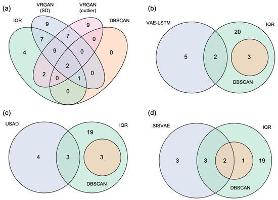
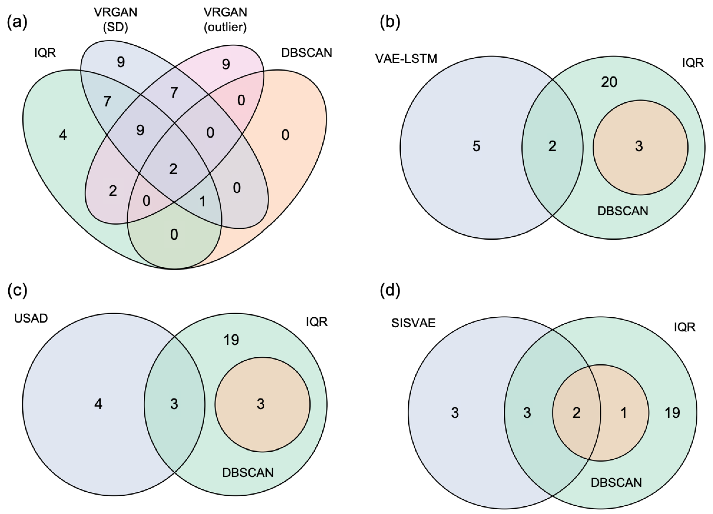
To validate the fidelity of the anomalies detected by our proposed model, we conducted several analyses and compared the results with baseline methods. First, we examined the overlap between the identified anomalous timepoints and outliers detected by the statistical methods (DBSCAN and IQR rules). VRGAN showed substantial overlap, identifying most outliers (100% for DBSCAN, 84% for IQR). In contrast, baseline methods had limited success, with only 12% of IQR outliers detected, and VAE-LSTM and USAD failing to detect any DBSCAN outliers (Figure 3).

Figure 3. Venn diagrams showing the overlap between anomalous timepoints detected by each method and outliers identified using the DBSCAN and IQR rules: (a) VRGAN; (b) VAE-LSTM; (c) USAD; and (d) SISVAE.

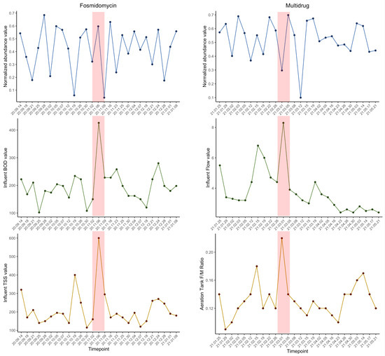
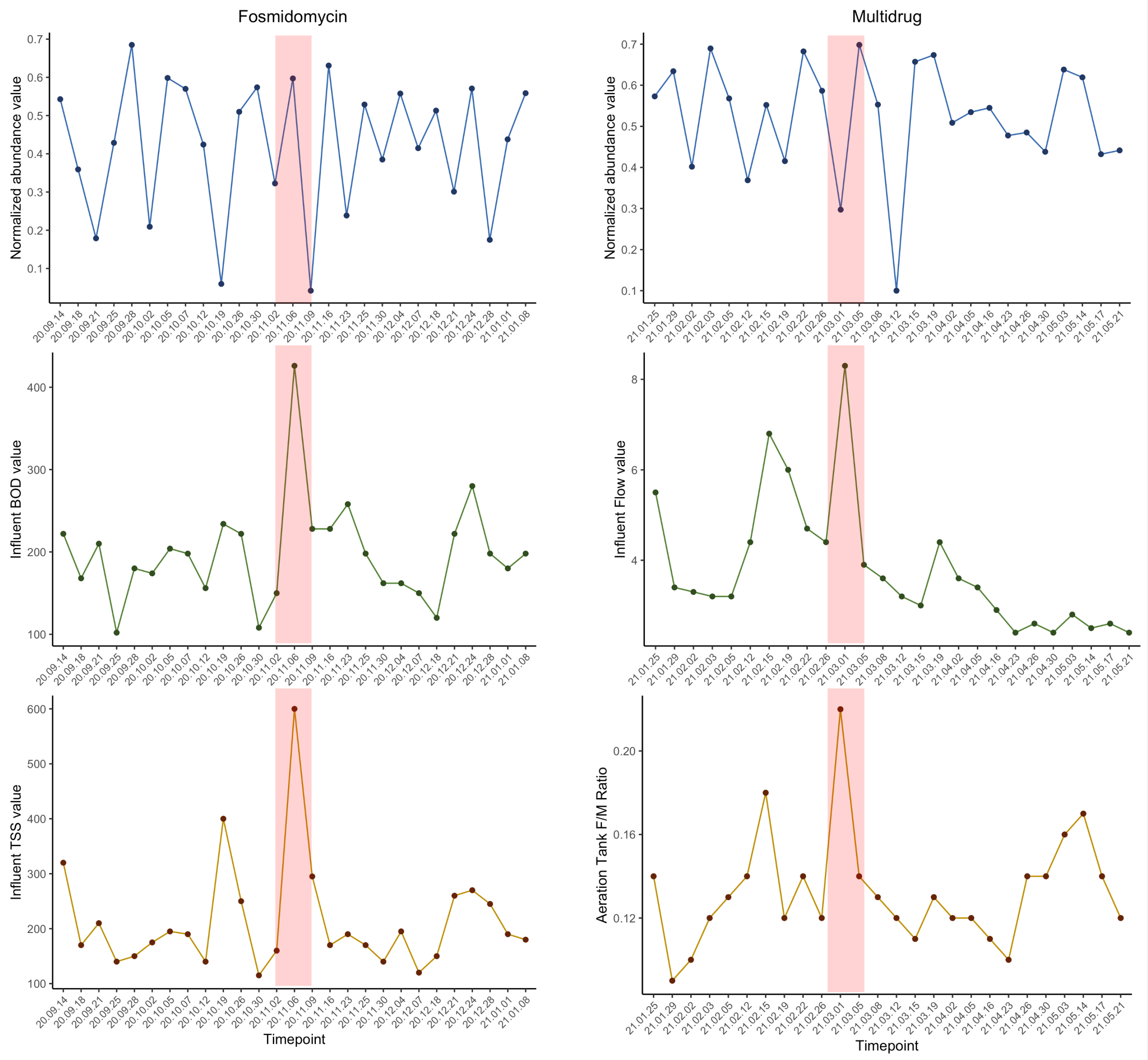
Next, we investigated whether anomalous timepoints identified solely by our model were associated with other water quality indicators at the time of sampling. Metadata, comprising 19 water quality parameters collected during the sampling for each timepoint, was used to detect outliers based on IQR rules. Those outliers were compared with the identified anomalous timepoints to infer whether the abnormality of ARG abundance could possibly relate to other measurable changes in water quality, as has been shown in other studies [33,34]. Fourteen timepoints were identified as anomalous first from VRGAN and subsequently compared with the corresponding metadata (Supplementary Material S5 and S6, Figure 4). In many cases, there were other notable changes in water quality that overlapped with anomalous points identified by VRGAN. For instance, for the timepoint of November 6th, 2020, identified as anomalous in ARGs encoding resistance to the Fosmidomycin drug class, we could see that TSS and BOD parameters in the influent peaked at their highest value of 600 and 426, respectively, compared with each of their averages of 225 and 216, which coincided with abnormal ARG relative abundances. TSS has been reported by others to be associated with antibiotic resistance in bacteria and BOD is a factor that can influence ARG occurrence [35]. Moreover, the timepoint of March 1st, 2021, was predicted as an anomaly in the multidrug ARG class, where we might get clues for this from the metadata variable of the FLOW parameter in the influent and F/M parameter in the aeration tank having a high value of 8.3 and 0.22, respectively, compared with their average of 3.63 and 0.14.

Figure 4. Visualization of the timepoints identified as anomalous only by VRGAN and their corresponding water quality metadata. The red-shaded regions indicate timepoints identified as outliers in the water quality metadata using the IQR rule.

In addition, we performed statistical testing to determine whether the anomalous timepoints we detected also deviate from a normal data distribution. We set a window of the size of five timepoints to include at least one anomaly detected by the model. Windows of the same size containing only samples identified as normal by the model were also set. Then, dynamic time warping (DTW), which is used to compare the similarity between the time series, was measured between the normal window pairs, and we also measured DTW between the pairs of normal windows and the anomalous window. After that, we checked whether the DTW between the anomalous and the normal windows was significantly different from the DTW measured between the normal pairs using the Wilcoxon rank-sum test. Statistical testing based on the anomaly detection results from our models and IQR achieved a p-value $<0.001$, and SISVAE and DBSCAN had a p-value less than 0.01 (Table 8). However, USAD and VAE-LSTM was not significantly different (p-value $>0.05$). This is likely stemmed from the assumption that the training dataset only contains normally distributed timepoints, leading to a high rate of false negatives.

Table 8. p-value results for statistical testing based on the DTW measured between the pairs of normal and anomaly windows and the DTW between the normal pairs.

	VRGAN (S.D.)	VRGAN (Outlier)	SISVAE	VAE-LSTM	USAD	IQR	DBSCAN
p-value	<$0.001$	<$0.001$	<$0.01$	0.955	0.924	<$0.001$	<$0.01$

4. Discussion

In this study, we developed and systematically evaluated VRGAN, a deep generative framework for unsupervised anomaly detection in multivariate time-series data. The primary methodological contribution of VRGAN lies in the integration of four complementary components: (1) label-free anomaly candidate identification and masking to mitigate training-data contamination, (2) sequential training of a variational recurrent neural network (VRNN) and a generative adversarial network (GAN), (3) dual reconstruction-based anomaly scoring, and (4) a validation-derived threshold that does not require ground-truth anomaly labels. Unlike conventional VAE- and recurrent reconstruction-based approaches that rely on their respective reconstruction mechanisms, VRGAN employs a two-stage generative architecture. The VRNN first learns temporal dependencies and stochastic latent representations, which are subsequently transferred to the GAN module. During the second training stage, the VRNN parameters are frozen, allowing the GAN to learn an additional reconstruction without modifying the pretrained VRNN. Furthermore, potential anomalous timepoints are identified using either the Z-score-based strategy or the combined DBSCAN–IQR method and masked during training to reduce their influence on the learned representations. Rather than relying on a single reconstruction output, VRGAN combines the reconstruction errors obtained from both modules to calculate anomaly scores. The detection threshold is subsequently determined using anomaly candidate information from the validation set without requiring ground-truth anomaly labels.

The benchmark evaluation demonstrated that VRGAN achieved competitive anomaly detection performance across datasets with different temporal characteristics and anomaly patterns. Specifically, VRGAN obtained the highest mean F1-scores among the evaluated methods on Yahoo-A1, SKAB-valve1, and TEP. In particular, VRGAN consistently achieved higher mean F1-scores than the newly included recurrent generative baselines, including VRNN-GRU, VAE-RNN, and GAN-RNN, across the evaluated datasets. On SMAP, MSL, and SMD, the VRGAN variants achieved the highest mean F1-scores under both point-wise and point-adjusted (PA) evaluation protocols, demonstrating that their relative performance was maintained regardless of whether PA was applied. These comparisons included recurrent generative models, autoencoder-based approaches, GAN-based methods, and Transformer-based architectures, providing a broad assessment against different modeling strategies.

The component ablation experiments provide further empirical evidence supporting the effectiveness of the integrated VRNN–GAN framework. Removing the GAN component decreased the mean AUROC across all four evaluated ablation datasets, supporting the contribution of incorporating GAN-based reconstruction alongside VRNN-based reconstruction into the complete detection pipeline. In contrast, the effects of anomaly candidate masking and smoothness regularization were more dataset-dependent, suggesting that their contributions vary according to the underlying temporal dynamics and anomaly characteristics. Together, these findings support the effectiveness of integrating the proposed components.

A key component of VRGAN is its label-free anomaly candidate identification and masking strategy, which aims to reduce the influence of potentially anomalous observations during model training. Unlike methods that assume anomaly-free training data or require labeled anomalies, VRGAN identifies potential anomalies using statistical criteria and adaptively determines the masking proportion according to the selected observations. The ablation experiments demonstrated that removing masking decreased the mean AUROC across all four evaluated datasets, with substantially larger reductions observed on the two SKAB datasets than on SMAP and MSL. These findings suggest that masking can improve detection performance by limiting the influence of potentially contaminated observations. The hyperparameter sensitivity experiments further showed relatively limited AUROC variation within the investigated ranges of the Z-score and DBSCAN–IQR parameters, indicating that the candidate-identification strategies were reasonably robust under the examined configurations.

The proposed label-free threshold determination strategy represents another key aspect of VRGAN, as threshold selection remains a critical challenge in unsupervised anomaly detection. VRGAN determines the decision threshold using the maximum validation anomaly score among observations not identified as anomaly candidates, thereby avoiding direct optimization against ground-truth anomaly labels. The threshold sensitivity experiments showed that the original validation-derived threshold achieved competitive F1-scores across the examined SKAB configurations. However, decreasing the threshold improved F1-scores for certain combinations of datasets and candidate-identification strategies, whereas increasing the threshold substantially reduced recall and F1-score. These results highlight the trade-off between precision and recall and demonstrate that the proposed threshold should be interpreted as a reproducible, label-independent operating point rather than a universally optimal decision boundary.

The anomaly-scoring mechanism of VRGAN combines the reconstruction errors obtained from the VRNN and GAN modules with equal weights. This design directly measures deviations between observed values and reconstructions generated through two different generative mechanisms. Alternative scoring strategies, including latent-space and discriminator-based scores, may capture different aspects of anomalous behavior. For example, latent-space scores may reflect deviations from learned representation distributions, whereas discriminator-based scores may provide information about the distinction between observed and generated sequences. However, their effectiveness depends on the learned latent distributions, discriminator behavior, and calibration of the resulting scores. Furthermore, combining heterogeneous scores introduces additional challenges in determining appropriate fusion weights without labeled validation data. Therefore, the proposed equal-weight reconstruction-based score represents a practical design choice consistent with the fully unsupervised objectives of VRGAN rather than a theoretically optimal scoring formulation.

To investigate the applicability of VRGAN beyond conventional engineering benchmarks, we further evaluated the framework using the CIWARS wastewater metagenomic time series, which lacks ground-truth anomaly labels. Wastewater surveillance presents a challenging anomaly detection setting because microbial and antibiotic resistance gene (ARG) abundance profiles can be influenced by environmental conditions, seasonal variations, and measurement variability. Following an analysis of the association between ARG abundance and wastewater temperature, the abundance data were differenced before anomaly detection to reduce potential seasonal confounding. VRGAN identified anomalous timepoints that overlapped with all DBSCAN outliers and 84% of IQR outliers, while several detections coincided with unusual water-quality measurements. In addition, dynamic time warping analysis revealed significant differences between the selected normal and anomalous windows for both VRGAN variants. Together, these observations provide evidence that the identified timepoints exhibit unusual temporal characteristics and warrant further investigation.

Despite the promising results, two main limitations should be acknowledged. First, the effectiveness of VRGAN depends on the reliability of anomaly candidate identification and threshold determination, which may be affected by data contamination and distribution shifts. Second, although VRGAN demonstrated competitive performance across multiple benchmark datasets, its generalizability to diverse real-world environments requires further validation, particularly in applications where ground-truth anomaly labels are unavailable. Future work will focus on developing more robust candidate identification and adaptive thresholding strategies, as well as extending the evaluation to additional real-world datasets. Nevertheless, the proposed framework demonstrates the potential of integrating label-free anomaly candidate masking, sequential VRNN–GAN training, and complementary reconstruction-based scoring into a unified anomaly detection pipeline. By eliminating the need for annotated training and validation data, VRGAN offers a promising approach for multivariate time-series anomaly detection in practical monitoring applications where reliable anomaly labels are difficult or costly to obtain.

References

- Xu, H.; Chen, W.; Zhao, N.; Li, Z.; Bu, J.; Li, Z.; Liu, Y.; Zhao, Y.; Pei, D.; Feng, Y.; et al. Unsupervised anomaly detection via variational auto-encoder for seasonal kpis in web applications. In Proceedings of the 2018 World Wide Web Conference, Lyon, France, 23–27 April 2018; pp. 187–196. [Google Scholar]
- Yan, J.; Tian, C.; Huang, J.; Albertao, F. Incremental dictionary learning for fault detection with applications to oil pipeline leakage detection. Electron. Lett. 2011, 47, 1198–1199. [Google Scholar] [CrossRef] [Scilit]
- Lewis, J.; Bartlett, A.; Atkinson, P. Hidden in the middle: Culture, value and reward in bioinformatics. Minerva 2016, 54, 471–490. [Google Scholar] [CrossRef] [Scilit]
- Venzon, M.; Bernard-Raichon, L.; Klein, J.; Axelrad, J.E.; Zhang, C.; Hussey, G.A.; Sullivan, A.P.; Casanovas-Massana, A.; Noval, M.G.; Valero-Jimenez, A.M.; et al. Gut microbiome dysbiosis during COVID-19 is associated with increased risk for bacteremia and microbial translocation. bioRxiv 2021. [Google Scholar] [CrossRef] [Scilit]
- Pietras, C.M.; Power, L.; Slonim, D.K. aTEMPO: Pathway-Specific Temporal Anomalies for Precision Therapeutics. In Proceedings of the Pacific Symposium on Biocomputing 2020; World Scientific: Singapore, 2019; pp. 683–694. [Google Scholar]
- Daughton, C.G. Wastewater surveillance for population-wide Covid-19: The present and future. Sci. Total Environ. 2020, 736, 139631. [Google Scholar] [CrossRef] [Scilit]
- Jumutc, V.; Suykens, J.A. Multi-class supervised novelty detection. IEEE Trans. Pattern Anal. Mach. Intell. 2014, 36, 2510–2523. [Google Scholar] [CrossRef] [Scilit]
- Kim, S.; Choi, Y.; Lee, M. Deep learning with support vector data description. Neurocomputing 2015, 165, 111–117. [Google Scholar] [CrossRef] [Scilit]
- Erfani, S.M.; Baktashmotlagh, M.; Moshtaghi, M.; Nguyen, V.; Leckie, C.; Bailey, J.; Ramamohanarao, K. From shared subspaces to shared landmarks: A robust multi-source classification approach. In Proceedings of the Thirty-First AAAI Conference on Artificial Intelligence, San Francisco, CA, USA, 4–9 February 2017. [Google Scholar]
- Su, Y.; Zhao, Y.; Niu, C.; Liu, R.; Sun, W.; Pei, D. Robust anomaly detection for multivariate time series through stochastic recurrent neural network. In Proceedings of the 25th ACM SIGKDD International Conference on Knowledge Discovery & Data Mining, Anchorage, AK, USA, 4–8 August 2019; pp. 2828–2837. [Google Scholar]
- Lin, S.; Clark, R.; Birke, R.; Schönborn, S.; Trigoni, N.; Roberts, S. Anomaly detection for time series using vae-lstm hybrid model. In Proceedings of the ICASSP 2020-2020 IEEE International Conference on Acoustics, Speech and Signal Processing (ICASSP); IEEE: Piscataway, NJ, USA, 2020; pp. 4322–4326. [Google Scholar]
- Audibert, J.; Michiardi, P.; Guyard, F.; Marti, S.; Zuluaga, M.A. Usad: Unsupervised anomaly detection on multivariate time series. In Proceedings of the 26th ACM SIGKDD International Conference on Knowledge Discovery & Data Mining, Virtual, 6–10 July 2020; pp. 3395–3404. [Google Scholar]
- Li, L.; Yan, J.; Wang, H.; Jin, Y. Anomaly detection of time series with smoothness-inducing sequential variational auto-encoder. IEEE Trans. Neural Netw. Learn. Syst. 2020, 32, 1177–1191. [Google Scholar] [CrossRef] [Scilit]
- Kim, S.; Choi, K.; Choi, H.S.; Lee, B.; Yoon, S. Towards a rigorous evaluation of time-series anomaly detection. In Proceedings of the AAAI Conference on Artificial Intelligence, Online, 22 February–1 March 2022; Volume 36, pp. 7194–7201. [Google Scholar]
- Huet, A.; Navarro, J.M.; Rossi, D. Local Evaluation of Time Series Anomaly Detection Algorithms. In Proceedings of the 28th ACM SIGKDD Conference on Knowledge Discovery and Data Mining, Washington, DC, USA, 14–18 August 2022; pp. 635–645. [Google Scholar]
- Khan, K.; Rehman, S.U.; Aziz, K.; Fong, S.; Sarasvady, S. DBSCAN: Past, present and future. In Proceedings of the Fifth International Conference on the Applications of Digital Information and Web Technologies (ICADIWT 2014); IEEE: Piscataway, NJ, USA, 2014; pp. 232–238. [Google Scholar]
- Chung, J.; Kastner, K.; Dinh, L.; Goel, K.; Courville, A.C.; Bengio, Y. A recurrent latent variable model for sequential data. In Proceedings of the 29th International Conference on Neural Information Processing Systems, Montreal, Canada, 7–12 December 2015; pp. 2980–2988. [Google Scholar]
- Kingma, D.P.; Ba, J. Adam: A method for stochastic optimization. arXiv 2014, arXiv:1412.6980. [Google Scholar]
- Yahoo’s A Labeled Anomaly Detection Dataset S5. Available online: https://huggingface.co/datasets/YahooResearch/ydata-labeled-time-series-anomalies-v1_0 (accessed on 21 April 2022).
- Katser, I.D.; Kozitsin, V.O. Skoltech Anomaly Benchmark (SKAB). 2020. Available online: https://www.kaggle.com/dsv/1693952 (accessed on 21 April 2022).
- Rieth, C.A.; Amsel, B.D.; Tran, R.; Cook, M.B. Additional Tennessee Eastman Process Simulation Data for Anomaly Detection Evaluation. 2017. Available online: https://dataverse.harvard.edu/dataset.xhtml?persistentId=doi:10.7910/DVN/6C3JR1 (accessed on 21 April 2022).
- Hundman, K.; Constantinou, V.; Laporte, C.; Colwell, I.; Soderstrom, T. Detecting spacecraft anomalies using lstms and nonparametric dynamic thresholding. In Proceedings of the 24th ACM SIGKDD International Conference on Knowledge Discovery & Data Mining, London, UK, 19–23 August 2018; pp. 387–395. [Google Scholar]
- Brown, C.L.; Rumi, M.A.; McDaniel, L.; Maile-Moskowitz, A.; Sein, J.; Nguyen, L.; Choi, M.; Hindi, F.; Mullet, J.; Emon, M.; et al. Metagenomics disentangles epidemiological and microbial ecological associations between community antibiotic use and antibiotic resistance indicators measured in sewage. medRxiv 2024. [Google Scholar] [CrossRef] [Scilit]
- Arango-Argoty, G.; Garner, E.; Pruden, A.; Heath, L.S.; Vikesland, P.; Zhang, L. DeepARG: A deep learning approach for predicting antibiotic resistance genes from metagenomic data. Microbiome 2018, 6, 23. [Google Scholar] [CrossRef] [Scilit]
- Pedregosa, F.; Varoquaux, G.; Gramfort, A.; Michel, V.; Thirion, B.; Grisel, O.; Blondel, M.; Prettenhofer, P.; Weiss, R.; Dubourg, V.; et al. Scikit-learn: Machine learning in Python. J. Mach. Learn. Res. 2011, 12, 2825–2830. [Google Scholar]
- Majeed, H.J.; Riquelme, M.V.; Davis, B.C.; Gupta, S.; Angeles, L.; Aga, D.S.; Garner, E.; Pruden, A.; Vikesland, P.J. Evaluation of metagenomic-enabled antibiotic resistance surveillance at a conventional wastewater treatment plant. Front. Microbiol. 2021, 12, 657954. [Google Scholar] [CrossRef] [Scilit]
- Zhang, Z.; Zhang, Q.; Wang, T.; Xu, N.; Lu, T.; Hong, W.; Penuelas, J.; Gillings, M.; Wang, M.; Gao, W.; et al. Assessment of global health risk of antibiotic resistance genes. Nat. Commun. 2022, 13, 1553. [Google Scholar] [CrossRef] [Scilit]
- Sun, W.; Qian, X.; Gu, J.; Wang, X.J.; Duan, M.L. Mechanism and effect of temperature on variations in antibiotic resistance genes during anaerobic digestion of dairy manure. Sci. Rep. 2016, 6, 30237. [Google Scholar] [CrossRef] [Scilit]
- Sui, Q.; Zhang, J.; Tong, J.; Chen, M.; Wei, Y. Seasonal variation and removal efficiency of antibiotic resistance genes during wastewater treatment of swine farms. Environ. Sci. Pollut. Res. 2017, 24, 9048–9057. [Google Scholar] [CrossRef] [Scilit]
- Schages, L.; Wichern, F.; Kalscheuer, R.; Bockmühl, D. Winter is coming–Impact of temperature on the variation of beta-lactamase and mcr genes in a wastewater treatment plant. Sci. Total Environ. 2020, 712, 136499. [Google Scholar] [CrossRef] [Scilit]
- Seabold, S.; Perktold, J. statsmodels: Econometric and statistical modeling with python. In Proceedings of the 9th Python in Science Conference, Austin, TA, USA, 28 June–3 July 2010. [Google Scholar]
- Petelin, G.; Cenikj, G.; Eftimov, T. Towards understanding the importance of time-series features in automated algorithm performance prediction. Expert Syst. Appl. 2023, 213, 119023. [Google Scholar] [CrossRef] [Scilit]
- Wang, J.; Mao, D.; Mu, Q.; Luo, Y. Fate and proliferation of typical antibiotic resistance genes in five full-scale pharmaceutical wastewater treatment plants. Sci. Total Environ. 2015, 526, 366–373. [Google Scholar] [CrossRef] [Scilit]
- Pallares-Vega, R.; Blaak, H.; van der Plaats, R.; de Roda Husman, A.M.; Leal, L.H.; van Loosdrecht, M.C.; Weissbrodt, D.G.; Schmitt, H. Determinants of presence and removal of antibiotic resistance genes during WWTP treatment: A cross-sectional study. Water Res. 2019, 161, 319–328. [Google Scholar] [CrossRef] [Scilit]
- Teban-Man, A.; Szekeres, E.; Fang, P.; Klümper, U.; Hegedus, A.; Baricz, A.; Berendonk, T.U.; Pârvu, M.; Coman, C. Municipal wastewaters carry important carbapenemase genes independent of hospital input and can mirror clinical resistance patterns. Microbiol. Spectr. 2022, 10, e02711-21. [Google Scholar] [CrossRef] [Scilit]
Disclaimer/Publisher’s Note: The statements, opinions and data contained in all publications are solely those of the individual author(s) and contributor(s) and not of MDPI and/or the editor(s). MDPI and/or the editor(s) disclaim responsibility for any injury to people or property resulting from any ideas, methods, instructions or products referred to in the content. |
© 2026 by the authors. Licensee MDPI, Basel, Switzerland. This article is an open access article distributed under the terms and conditions of the Creative Commons Attribution (CC BY) license.