


Featured Application
The model sizes a construction robot fleet and assigns it to activities on a project schedule, so that a contractor can decide how many machines to hold, which trades to give them, and how to keep crews clear of them before the machines arrive on site.
Abstract
Construction robots for repetitive trades have moved beyond demonstration, yet fleet size and task assignment are still decided by rule of thumb. This study formulates the human–robot collaborative resource-constrained project scheduling problem, which chooses execution modes, fleet size, and start times together and renders the speed-and-separation requirement as a static zone-exclusivity constraint. A heuristic, repair-augmented evolutionary method is validated against exact bi-objective fronts and two established heuristics. In computational experiments on 30 generated apartment-finishing instances of 64 to 128 activities, the minimum-cost schedule reduced cost by 3.7% relative to a human-only plan, whereas robotizing every eligible activity cost 7.8% more than using no robots at the calibrated day rate and paid off only below about 649 thousand KRW per machine-day. As skilled-labor availability fell to 40%, the cost effect of a two-machine fleet moved from −2.2% to +17.0%, and a factorial design attributed more of the variance in cost saving to labor availability than to machine productivity. Static zone exclusivity lengthened the schedule by 11.0%, an upper bound on the cost of dynamic separation. Under duration noise and downtime the schedule advantage persisted while the cost advantage narrowed. All results are model-based estimates conditional on the calibrated assumptions.
1. Introduction
Construction has long been organized on the assumption that skilled trades will be available when the schedule calls for them. That assumption is weakening. In an analysis of 97 North American projects, Karimi et al. found that sites facing craft shortages had lower labor productivity and longer schedules [1], and the same data linked shortages to poorer safety performance [2]. Elbashbishy and El-adaway later showed that the shortage has become structural across labor-intensive trades in both union and nonunion settings [3]. The classical remedy—adding crews to protect the completion date—fails precisely when there are no crews to add.
Over the same period, construction robots have moved past proof of concept. The technological trajectory of construction automation and of robot-oriented design has been mapped systematically [4,5], and quantitative evidence is accumulating. Comparing a straight and a double-curved reinforced concrete wall built by digital fabrication with conventional formwork, García de Soto et al. showed that the productivity advantage of the robotic process is conditional: it appears only as geometric complexity rises [6]. Machines for masonry, board fixing, painting, and layout are now on sites, but diffusion remains slow, and the barrier is economic rather than technical. In a mixed-method study with 28 experts, the highest-ranked obstacle was high initial capital investment [7]; an analysis of the United States industry reached the same conclusion and added the scarcity of qualified operators [8].
1.1. The Deployment Decision on Site
If the binding constraint is economic, what is needed is not a better machine but a better deployment decision. Three questions confront the site manager: how many machines to hold for the project, which activities to give them, and how to arrange the remaining crews around them. The three are not separable. Enlarging the fleet shortens individual activities but incurs a holding cost for the whole project, so the penalty grows with the very schedule it is meant to shorten. Assigning more activities to robots raises utilization but lengthens the queue in front of the machines, and the schedule can end up longer than it would have been without them. Each decision therefore has to be taken on the project network rather than activity by activity.
The literature approaches this space from two sides and leaves the middle empty. One stream examines adoption—barriers, competencies, willingness—at the level of the firm [7,8]. The other develops perception, control, and motion planning for individual machines, plans their paths, or allocates tasks among several of them [9,10,11,12,13]. The first asks whether to adopt, the second how to move. Between them lies the question of how many machines to hold and where to put them, which belongs to resource-constrained project scheduling (RCPSP). Existing RCPSP extensions, however, treat resource availability as an exogenous constant, whether the modeled flexibility lies in execution modes [14] or in workforce skills [15,16,17], and none of them represents the spatial separation that operating a robot beside a human crew requires.
1.2. Problem Statement and Propositions
This study asks three questions. (RQ1) Does the intuitive policy of applying robots wherever they are technically applicable improve project outcomes at the day rates that commercial machines currently command? (RQ2) How much of the value of a robot fleet is governed by the productivity of the machine, how much by its price, and how much by the scarcity of the labor it displaces? (RQ3) What does the safety separation required around an operating robot cost at the level of the schedule? Three propositions follow, each stated with the condition under which it is examined.
- P1.
- At the calibrated machine day rate, applying robots to every eligible activity is dominated: it raises total cost relative to a human-only plan without shortening the schedule. The proposition is conditional on price, and the price below which it ceases to hold is identified.
- P2.
- Holding the machine, its price and the project network constant, the sign of the cost effect of robot deployment is governed by the availability of the skilled labor the machine displaces; and in a factorial design that varies availability, productivity and price together, availability accounts for a share of the variance in cost saving that is at least comparable to that of productivity.
- P3.
- The zone exclusivity required by collaborative-robot safety practice, rendered as a static exclusion at the resolution of a daily schedule, imposes a measurable schedule and cost penalty that is large enough to enter the deployment decision.
1.3. Contributions and Structure of the Paper
The study makes three kinds of contribution, which we keep separate because they rest on different evidence.
- Modeling. We formulate the human–robot collaborative resource-constrained project scheduling problem (HRC-RCPSP). The execution mode of every activity, the number of machines held, and the start times are decided jointly; the number of machines is a decision variable whose cost is proportional to the makespan it is used to shorten; and the speed-and-separation requirement of collaborative-robot practice is carried at schedule resolution as a zone-exclusivity constraint. Extensions with two machine types, rental-style holding windows, and temporary skilled hires are formulated and tested.
- Algorithmic. A serial schedule generation scheme with a delay-aware mode repair is embedded in a non-dominated sorting evolutionary algorithm. The method is validated against proven-optimal makespans of a discrete-time mixed-integer program, against complete bi-objective fronts obtained by the ε-constraint method at small scale, and against priority-rule sampling and simulated annealing at project scale. The components are established ones; the problem-specific element, the repair, is a greedy heuristic that carries no dominance guarantee, and its value is established computationally rather than proven.
- Managerial. We report computational results with direct decision content: the price threshold below which indiscriminate deployment stops being dominated, the dependence of the sign of the cost effect on labor availability, a break-even map over machine productivity and day rate, the marginal cost of a day of schedule along the front, and an upper bound on the schedule price of the safety rule. These are model-based estimates under calibrated assumptions, not field measurements, and the analysis states the conditions on which they rest: the price of the machine, the share of activities it can take, the coupling of the precedence network, and the level of duration uncertainty.
Section 2 reviews the literature and states the research gap. Section 3 presents the formulation, the solution method, and the experimental design; Figure 1 maps the inputs, the model, the two solution routes, the experimental campaign, and the outputs. Section 4 reports the results, Section 5 discusses them together with alternative explanations, boundary conditions, and limitations, and Section 6 concludes. Experiments that support the main results without changing them are reported in the Supplementary Materials.
Figure 1.
Inputs, model, solution routes, experimental campaign, and outputs of the study.
2. Literature Review
2.1. Productivity Evidence and Adoption Barriers
The technological lineage of construction automation is documented by Bock [4] and in the robot-oriented design framework of Bock and Linner [5]. Quantitative evidence on productivity is more recent and more guarded. García de Soto et al. found a robotic mesh-mould process inferior to conventional construction for a simple wall and superior for a complex one [6], and Pan et al. reported that the economic indicators of construction automation depend heavily on utilization and project scale [18]. The productivity advantage of a construction robot is thus conditional on what it is asked to do and how intensively it is used, which turns deployment into a planning problem rather than a purchasing one. Studies of adoption barriers agree: high initial capital investment ranks first among the obstacles reported by practitioners [7], and uncertainty over recovering that investment, together with the shortage of qualified operators, leads the constraints identified in the United States [8]. Both point past the machine toward the decision of how much of it to buy and where to use it.
2.2. Human–Robot Collaboration and Safety Separation
Human–robot collaboration in construction was given a structure by the review of Liang et al. [9] and has since extended to teaching quasi-repetitive tasks by demonstration [10] and to safety-constrained reinforcement-learning control [11]. On the safety side, the technical specification for collaborative robots names speed and separation monitoring as a principal risk-reduction method [19]; implementing it requires the protective separation distance to be recomputed continuously from the speeds of robot and operator [20], and sensor-based implementations have been demonstrated [21]. The manufacturing literature has examined how the requirement shapes collaborative assembly [22] and how the level of automation interacts with operator workload [23]. A recent review notes that the unstructured character of construction sites makes the manufacturing formulation hard to apply directly and proposes workspace-level separation as the realistic alternative [24]. The human side of the interaction has begun to enter scheduling: Tian and Yu optimized task schedules for efficiency and ergonomic load jointly [25], and Sam and Franz assessed the vulnerability of a collaborative drywall operation to uncertainty [26]. In both, the unit of analysis is a task or a crew, not the project network.
2.3. Task Allocation and Team Composition for Construction Robots
Allocation among several machines forms a separate stream. Ye et al. decomposed the allocation of multiple construction robots into two stages and solved it with an improved genetic algorithm [12]; the path-planning algorithms on which such allocations depend have been reviewed recently [13]; and Pan and Yu searched over the composition of heterogeneous robot teams for long-horizon tasks with time- and utilization-guided simulation [27]. Both decide how many machines of what kind to field, which is also our concern. In both, however, the human crews are a background condition: neither the aggregate availability of skilled labor nor the choice between a human and a robotic mode for the same activity is a decision variable. Where that availability binds, which is the situation this study addresses, their conclusions need not carry over.
2.4. Resource-Constrained Project Scheduling and Its Extensions
The RCPSP has accumulated four decades of variants, surveyed twice by Hartmann and Briskorn [28,29]. Standard libraries [30] and comparative evaluations of heuristics [31,32] provide the benchmarks against which a new method is expected to be placed: serial and parallel schedule generation with priority rules and biased random sampling [33], activity-list genetic algorithms [34], and, for the multi-mode case, the metaheuristic comparison of Van Peteghem and Vanhoucke [35]. The multi-mode extension itself was settled by the exact-algorithm comparison of Hartmann and Drexl [14]; objectives other than time, such as the financial optimization of a project with milestone payments [36], have been brought into the same frame; and scheduling under duration uncertainty has its own survey [37]. The multi-skill variant, which represents workforce competencies explicitly, runs from Bellenguez-Morineau and Néron [17] to the priority-rule heuristics and modeling-framework comparisons of Almeida et al. [15,16], and has recently been combined with schedule risk analysis [38] and with flexible resource profiles under multiple objectives [39]. Construction applications include genetic-algorithm scheduling of prefabricated projects [40], schedule compression under uncertainty [41], multi-objective scheduling of large repetitive works [42], and linear scheduling of works executed in reverse order [43]. Workspace interference has been modeled with a spatial conflict simulator [44], the closest precedent for the zone constraint used here.
2.5. Research Gap
Three gaps follow. First, robot allocation studies optimize the robot side while holding human crews fixed, so they cannot represent the substitution that deployment is meant to achieve [12,27]. Second, RCPSP extensions treat resource availability as given, which is untenable for a resource whose quantity is itself the dominant cost item [28,29]. Third, no study we are aware of quantifies what the separation required around an operating robot costs at the level of the schedule, although the requirement is stated normatively [19,24]. Table 1 places the principal prior studies against the decisions each of them makes. The present study treats mode assignment, fleet size, and sequencing as one problem, carries the safety separation as an explicit constraint, and reports the price of each.
Table 1.
Decision scope of the principal prior studies.
3. Materials and Methods
3.1. Research Design
The study follows the sequence of Figure 1. A formulation is derived from the deployment decision of Section 1.1. Small instances are solved to proven optimality—for the makespan at each fleet size and for the complete bi-objective front—so that the constraint handling and the search of the heuristic method can be checked against exact references. Realistically sized instances are then solved by the evolutionary method and by two established comparators, and the resulting fronts are examined under scenarios that vary labor availability, machine economics, the safety rule, and the modeling assumptions themselves. Every comparison is paired: within an instance, all policies face the same network, durations, and resource limits, so differences between policies cannot be attributed to differences in instance difficulty. All results are computational. No field data were collected, and the study is offered as a decision-support framework whose parameters are to be replaced by site measurements as they become available.
3.2. Problem Description and Assumptions
The following terms are used throughout. A trade is a craft category (masonry, tiling, painting). An activity is the work of one trade on one work unit. A crew is the set of workers that executes one activity, described by its numbers of skilled and general workers; skilled workers are trade-qualified craft workers, and general workers provide handling and assistance. An operator is the single certified worker, drawn from the skilled pool, who supervises a machine in the robot-led mode. A machine or robot is one unit of construction robotic equipment, and the fleet is the number of machines held for the project.
A project consists of a finite set of activities defined on work units—dwellings, in the case treated here. Several adjacent units form one safety zone, much as dwellings on one floor share a working space; the zone is deliberately coarser than the unit because the reach of a machine and the separation it requires do not stop at the boundary of a dwelling. Every activity is executed in one of three modes—human-only (H), collaborative (C), or robot-led (A)—and the modes available depend on the trade. Modes C and A both occupy a machine and are referred to jointly as robot-based modes. The modeling assumptions are as follows.
- A1.
- Activities are not preempted once started.
- A2.
- The execution mode is fixed at the start of an activity and does not change during it.
- A3.
- Skilled and general labor are each available up to a constant ceiling for the duration of the project. In the baseline the ceilings are inputs; an extension in which the skilled ceiling can be raised by temporary hires at a wage premium is examined in Section 4.4.
- A4.
- In the baseline, robots are acquired at project start, held until completion, and generate a holding cost over the whole project duration and a variable cost over the days on which they actually work. A rental-style variant in which the holding cost accrues only over the window between the first and the last robot activity, plus a mobilization fee, is examined in Section 4.8.
- A5.
- No other crew enters a safety zone while a robot is operating in it.
- A6.
- Relocation and setup of a machine are charged as a fixed allowance per activity, independent of the order in which the machine visits units.
- A7.
- Charging and servicing are represented by a duty-cycle factor applied to the processing time. Durations are deterministic in the baseline; the consequences of duration noise and machine downtime for a planned schedule are examined in Section 4.8.
A4 is where the formulation departs from the standard RCPSP. In the classical problem the availability of a renewable resource is a constant; for a machine being introduced into an operation, that availability is the principal cost decision and must be endogenous. Whole-project holding is the conservative case for the machine, since it charges every day between acquisition and completion, as an owned machine or a fixed-term lease would; Section 4.8 measures how much of that charge a holding window matched to the robot activities removes.
A5 renders the speed-and-separation requirement of collaborative-robot practice [19,21] at the resolution of a daily schedule. The specification itself is dynamic: the protective separation distance is recomputed continuously from the speeds of the robot and of the nearest person, and co-presence is permitted whenever that distance is maintained [20]. A daily schedule cannot represent that dynamic, and an unstructured construction site, with crews moving material through shared spaces, cannot yet supply the sensing on which it rests [24]. A5 therefore replaces the dynamic rule with a static one: while a machine operates in a zone, no other crew enters it. The approximation is conservative in one direction only. Every schedule feasible under A5 is feasible under the specification, but not conversely, so the penalty measured in Section 4.6 is an upper bound on what the separation requirement costs at schedule resolution; the zone-granularity experiment in the same section shows how the bound moves as the exclusion is narrowed.
3.3. Notation
Table 2 lists the sets, parameters, and decision variables of the formulation; the additional symbols of the model extensions are introduced where they appear in Section 3.6.5.
Table 2.
Sets, parameters, and decision variables.
3.4. Mode Durations and Crew Requirements
The human-only duration d_iH follows from the standard productivity of the trade. The two robot-based durations are obtained from it through the productivity multiplier ρ_i, the duty-cycle factor η, and the setup allowance σ, as in Equations (1) and (2).
d_iC = ⌈ (d_iH/(1 + λ(ρ_i − 1)))/η + σ ⌉
d_iA = ⌈ (d_iH/ρ_i)/η + σ ⌉
The multiplier ρ_i is drawn for every activity from the calibrated distribution of Section 3.8, so that machines of the same type differ in realized performance from one activity to the next. A trade-specific multiplier would be a refinement that the available evidence does not yet support: published comparisons report ranges for single processes rather than distributions by trade [6,27]. The coefficient λ ∈ (0, 1) is the share of the machine’s potential gain that the collaborative mode realizes; in collaboration the pace remains partly set by the worker, so only part of the gain is captured, as both the ergonomic-scheduling and the field-case literature report [25,26]. With λ = 0.55 the collaborative duration lies roughly midway between the human-only and the robot-led duration; Section S3 of the Supplementary Materials reports the results at 0.35 and 0.75. On the resource side, the crew of each mode follows a fixed rule from the human-only crew (s_iH, g_iH) of Table 3. Mode C releases one skilled worker and keeps the general labor: s_iC = max(1, s_iH − 1), g_iC = g_iH. Mode A replaces the skilled crew with a single certified operator and retains two general workers for material handling: s_iA = 1, g_iA = 2. The resulting requirements are listed by trade in Table 3. The three modes correspond to distinct levels of automation in the sense of the human–robot interaction literature [23], and robots substitute for skilled labor partially rather than entirely, as field evidence reports [6,26].
Table 3.
Trade data, crew requirements by mode, and robot applicability.
3.5. Mixed-Integer Formulation
A discrete-time formulation is used. The two objectives, makespan and total cost, are given by Equations (3) and (4).
min f1 = C_max
min f2 = Σ_i Σ_m Σ_t d_im (s_im w_S + g_im w_G) x_imt + c_F K C_max + c_V Σ_i Σ_m Σ_t r_im d_im x_imt + c_O C_max
The second term of Equation (4) is the holding cost of the fleet over the project duration and the third is the variable cost of the days actually worked. Separating them matters: with a holding cost alone, keeping every machine busy is always weakly optimal and indiscriminate deployment looks efficient by construction. The constraints are Equations (5)–(14).
Σ_{m∈M_i} Σ_{t∈T} x_imt = 1, ∀ i ∈ A
Σ_m Σ_t (t + d_im) x_imt ≤ C_max, ∀ i ∈ A
Σ_m Σ_t t x_jmt ≥ Σ_m Σ_t (t + d_im) x_imt, ∀ (i, j) ∈ P
Σ_i Σ_m s_im Σ_{τ∈W(i,m,t)} x_imτ ≤ S, ∀ t ∈ T
Σ_i Σ_m g_im Σ_{τ∈W(i,m,t)} x_imτ ≤ G, ∀ t ∈ T
Σ_i Σ_m r_im Σ_{τ∈W(i,m,t)} x_imτ ≤ K, ∀ t ∈ T
Here W(i, m, t) = {τ ∈ T: t − d_im < τ ≤ t} is the set of start times that leave activity i in progress at t. Equation (5) assigns exactly one mode and one start time to every activity, Equation (7) enforces precedence, and Equations (8)–(10) impose the period-by-period ceilings on labor and machines. The safety requirement is carried by Equations (11)–(13) through the zone-occupancy indicator y_zt.
y_zt = Σ_{i∈A_z} Σ_{m: r_im=1} Σ_{τ∈W(i,m,t)} x_imτ, ∀ z ∈ Z, t ∈ T
y_zt ≤ 1, ∀ z ∈ Z, t ∈ T
Σ_{i∈A_z} Σ_{m: r_im=0} Σ_{τ∈W(i,m,t)} x_imτ ≤ κ_z (1 − y_zt), ∀ z ∈ Z, t ∈ T
Equation (11) defines y_zt as the number of robot-based activities in progress in zone z at time t, and Equation (12) admits at most one machine to a zone at a time, so y_zt is binary. Equation (13) is the exclusivity itself: when a machine is operating in the zone the right-hand side is zero and every concurrent human-only activity in that zone is blocked; when no machine is present, crews are admitted up to the zone capacity κ_z. The sets W(i, m, t) appear in every occupancy term, so each constraint applies to the activities actually in progress at t, not only to those starting at t. Equation (14) states the variable domains.
x_imt ∈ {0, 1}, y_zt ∈ {0, 1}, K ∈ Z+, C_max ≥ 0
The product of K and C_max in Equation (4) makes the cost objective bilinear when the fleet size is a variable. Both methods treat K as an outer variable. In the exact experiments the model is solved for each K from zero to an upper bound—for the makespan directly, and for the cost by the ε-constraint method with the makespan bounded from above—so every program solved is linear; the fronts obtained for the different fleet sizes are then merged and filtered for dominance. This is exact, not a linearization, because the practical range of K is small. In the evolutionary method K is a gene of the individual and Equation (4) is evaluated directly on the decoded schedule.
Equation (12) also bounds the useful fleet. Because at most one machine operates in a zone at a time, no more than |Z| machines can work simultaneously. Any schedule that is feasible with K > |Z| machines is therefore feasible with |Z| machines at the same makespan and, by the holding term of Equation (4), at a strictly lower cost, so solutions with K > |Z| are dominated and the admissible fleet range is 0, …, |Z|. The same argument applies to any fleet larger than the peak number of machines a schedule has in use. The evolutionary method treats K as a free gene between 0 and 6 and does not impose either bound, so a solution can carry an idle machine until a trimmed copy displaces it; Section 4.2 reports how often this occurs in the fronts of the main experiment.
Complexity
Restricting every activity to a single mode, setting the robot requirement to zero, and relaxing the zone capacity to the size of the zone reduces the HRC-RCPSP to the classical RCPSP, which is strongly NP-hard [45]. The problem inherits that status; the mode and fleet-sizing layers enlarge the search space rather than restrict it. Exact solution can therefore be expected only for small instances, which is what Section 4.1 observes, and the approximate method of Section 3.6 is a necessity rather than a convenience.
3.6. Solution Method
3.6.1. Representation and Schedule Generation
The number of binary variables in the discrete-time model grows with the product of activities, modes, and periods, so an approximate method is needed at realistic sizes. A solution is a triple: an activity permutation π, a mode vector μ, and a fleet size K. The permutation need not respect precedence; before decoding it is converted into a feasible activity list by repeatedly taking the eligible activity of highest rank. The decoder is a serial schedule generation scheme: activities are placed in list order at the earliest period, at or after the completion of their predecessors, at which the labor and machine profiles and the zone conditions of Equations (11)–(13) are all satisfied. The resulting schedule is always feasible and active.
3.6.2. Delay-Aware Mode Repair
One structural loss arises in decoding. When an activity is assigned a robot-based mode but no machine is free, or the zone is occupied, the activity waits; if the wait is long enough, it consumes the saving in processing time and the activity would have finished earlier in the human-only mode. Mutation corrects this only slowly, because the improvement requires changing one gene whose effect propagates through every later placement. The decoder therefore carries a delay-aware mode repair (DMR): for an activity assigned a robot-based mode, the earliest feasible start is computed for that mode and for the human-only mode, and the mode is reverted whenever waiting for the machine yields no earlier completion (Algorithm 1). The repaired mode also enters the cost evaluation, so the procedure removes the operating cost of machine-days that bought nothing.
| Algorithm 1. Serial schedule generation with delay-aware mode repair. |
| Input: activity list L, mode vector mu, fleet size K Output: start times Sx, realized modes mu*, makespan Cmax 1 initialize resource and zone occupancy profiles 2 for i in L do 3 m <- mu(i); est <- max{ F(j) : j in pred(i) } 4 t_m <- earliest feasible start of (i, m) at or after est 5 if r_im = 1 then 6 t_H <- earliest feasible start of (i, H) at or after est 7 if t_H + d_iH < t_m + d_im then m <- H; t_m <- t_H 8 end if 9 Sx(i) <- t_m; F(i) <- t_m + d_im; mu*(i) <- m 10 update profiles over [t_m, F(i)) 11 end for 12 Cmax <- max_i F(i) |
Lines 5–8 are the repair. Because the search for a feasible start advances period by period and is run for at most two modes, decoding costs at most twice as much as the plain scheme. The repair is a greedy, local rule: it compares completion times of the current activity only and ignores the possibility that a later activity might have used the machine more profitably, so it is not guaranteed to preserve the dominance relations of the population. Its effect on the front is therefore measured rather than assumed (Section 4.3), and a variant that applies the repair with probability one half is reported in Section S4 of the Supplementary Materials.
3.6.3. Bi-Objective Evolutionary Search
Makespan and cost conflict, so a non-dominated sorting search is used rather than a weighted sum. The skeleton follows NSGA-II [46]; the ε-constraint method [47] serves at the exact end, and preference-weighting schemes such as the analytic hierarchy process [48] were avoided so that the trade-off is reported rather than resolved by the analyst. Crossover is order-preserving one-point on the permutation and uniform on the mode vector, and K is inherited from one parent chosen at random. Mutation swaps permutation elements with probability 0.06 per position, resamples the mode of an activity with probability 0.08 per position, and shifts K by ±1 with probability 0.25 per individual. Selection is a binary tournament on non-domination rank and crowding distance, and survival is elitist over the merged parent and offspring populations. The population holds 40 individuals and evolves for 50 generations, a budget of 2000 schedule decodings (Table A1); Section 4.3 examines budgets from 500 to 9600. Half of the initial population is seeded with structured solutions—the human-only plan, the robot-maximal plan for every fleet size from zero to the upper bound, and a perturbation of each in which about a third of the robot-eligible activities are returned to the human-only mode—and the other half is random; Section 4.3 also reports the search from a fully random population. The first non-dominated front of the final population is reported, and front quality is summarized by the hypervolume indicator [49]. The indicator is computed on objectives normalized by the makespan and cost of the human-only plan, against a reference point common to all the fronts being compared on an instance and placed 5% beyond the worst value of each objective over those fronts, so that the reference point is dominated by every solution and every solution contributes to the indicator. Where a single representative is needed, the knee point is used: both objectives are normalized over the front and the solution closest to the ideal point in Euclidean distance is taken. The knee is a reporting device, not a recommendation; every comparison in Section 4 is also reported at the minimum-cost and minimum-makespan ends of the front, and Section 5.2 replaces the knee with the marginal cost of a day of schedule, which lets a manager select a solution from the value the contract attaches to time.
Two comparators from the project-scheduling literature are run on the same representation and decoder at the same budget of decodings: regret-based biased random sampling on the latest-finish-time priority rule [33], with modes and fleet size drawn at random and a non-dominated archive kept over the sample, and simulated annealing [50] on a weighted sum of the two normalized objectives, run for five weights with the budget divided equally among them and the archives merged. Both are standard baselines for activity-list metaheuristics [34,35].
3.6.4. Reference Policies
Four reference policies and a decomposition are computed on every instance of the main experiment. The rule-based human-only policy executes all activities in mode H under the latest-finish-time priority rule and represents current practice. The optimized human-only policy searches over the activity sequence alone with the same evolutionary algorithm, modes fixed at H and K fixed at zero; the difference between the two isolates the gain that comes from better sequencing and owes nothing to machines. The rule-based robot-maximal policy assigns the fastest available mode to every activity a machine can take and schedules it under the same priority rule; it is evaluated for every fleet size from one to the upper bound and the least-cost result is retained. It is not a proposal that anyone defends in print. It is the upper bound of deployment intensity, included because it is the operating principle that the barrier literature reports on early-adopting sites [7,8] and because its distance from the proposed solutions measures how much of the value of a fleet lies in restraint. To remove any handicap from the priority rule, an optimized robot-maximal policy searches over the sequence and the fleet size with the modes held at their fastest setting. Finally, a sequential two-stage procedure, of the kind used when scheduling and equipment decisions are taken by different parties, fixes the optimized human-only sequence and then chooses modes and fleet size by greedy cost descent on that sequence; the gap between it and the integrated solution is the value of deciding the three together.
3.6.5. Model Extensions
Four extensions are implemented in the same decoder and searched by the same algorithm, so that their effects can be compared with the baseline on identical instances. (i) Heterogeneous fleet: machines are of two types—a heavy type for masonry, board fixing, and plastering and a light type for layout, tiling, and painting—each with its own fleet size K_r; Equation (10) is stated per type and the holding term of Equation (4) becomes c_F C_max Σ_r K_r. (ii) Windowed holding: for each machine type the holding cost accrues from the first start to the last finish of the robot-based activities, S_r to F_r, and a mobilization fee φ is charged per machine, so the holding term becomes Σ_r K_r (c_F (F_r − S_r) + φ). (iii) Temporary skilled hires: an integer number h of additional skilled workers raises the ceiling S to S + h for the whole project at a wage w_S (1 + π) per day, where π is the hiring premium; h is a gene of the individual. (iv) Stochastic realization: a planned schedule—its activity order, realized modes, and fleet—is re-executed by the decoder with every duration multiplied by a lognormal factor of mean one and coefficient of variation ν, and with every robot-based activity extended by two days with probability p_d to represent a breakdown; the realized makespan and cost are averaged over 200 draws. The realization holds the plan fixed and does not re-optimize, so it measures the exposure of a plan to uncertainty rather than the value of re-planning.
3.7. Instance Generation
The test instances reproduce the structure of apartment finishing work. Each of U work units passes through eight trades in a fixed order, and the crew of a given trade moves from one unit to the next, so the precedence relations form a lattice of within-unit chains and between-unit flows (Figure 2). Two adjacent units form one safety zone, so the number of zones is half the number of units. The same lattice underlies published models of large repetitive construction [42].
Figure 2.
Unit–trade precedence lattice and its relation to safety zones (solid arrows: trade sequence within a unit; gray dashed arrows: flow of a trade between units; brackets: safety zones).
Trade data and robot applicability are given in Table 3. Applicability is graded from the trades addressed by machines that are commercially available or in field trials: masonry, board fixing, and painting admit robot-led execution; mechanical and electrical layout, plastering, and tiling admit collaboration only; window installation and final finishing are excluded. Base durations are perturbed by a uniform factor of ±15% across units.
Setting U to 8, 12, and 16 gives instances of 64, 96, and 128 activities, ten per size differing in random seed; these 30 instances form the main experiment. The scenario experiments of Section 4.4, Section 4.5, Section 4.6, Section 4.7 and Section 4.8 use ten instances of 64 activities, or ten of 80 activities where the scenario concerns labor availability, and the grid of Section 4.5 uses three. For the exact comparison, smaller instances of 16, 24, and 32 activities were generated, four per size.
The four instances per size (seeds 101–104) serve the makespan validation. For the bi-objective validation, which is confined to 16 activities, two further 16-activity instances (seeds 105 and 106) were generated, so that six instances are used there.
Because the instances are generated rather than observed, the quantities they imply are reported so that their plausibility can be judged. Summed over the eight trades, a dwelling carries 39.2 days of work; under the human-only plan the eight-unit instances complete in 116.8 days, a cycle of 14.6 days per dwelling once trades overlap across units; direct cost including site overhead is 68.0 million KRW per dwelling; and crew sizes of two to six workers against ceilings of twelve skilled and six general workers allow two to four trades to proceed at once. These are the magnitudes of a mid-rise apartment finishing package. A reader who judges them unrepresentative can rescale them: the results in Section 4 are reported as percentages, and Sections S2 and S3 of the Supplementary Materials show how they move when the underlying parameters are perturbed.
3.8. Parameter Calibration
Parameters were taken from published sources where these exist and made the subject of sensitivity analysis where they do not (Table 4). Wages follow the Korean construction wage survey [51]. The robot day rate was built up as follows. An acquisition price of 550 million KRW was assumed for a semi-autonomous machine of the masonry or board-fixing class, an order of magnitude consistent with the surveys that rank capital investment as the leading barrier to adoption [7,8]; straight-line recovery over five years at 220 working days a year gives 500 thousand KRW per machine-day. Insurance and scheduled maintenance at 12% of the price per year add 300, and transport and software subscriptions add 100, for a total of 900 thousand KRW per machine-day. Capital recovery, insurance, and the fixed part of maintenance (522, or 58%) are incurred whether or not the machine works and form the holding rate c_F; energy, consumables, wear-related maintenance, transport between workfaces, and software (378, or 42%) are incurred only on working days and form the operating rate c_V. Because the price of any particular machine can be argued, the day rate is swept from 300 to 1200 thousand KRW in Section 4.5, which covers a machine costing about 140 to 760 million KRW under the same recovery assumptions. The productivity multiplier follows a triangular distribution with mode 2.2 and bounds 1.5 and 3.0, consistent with the time comparisons reported for robotic fabrication [6] and for heterogeneous robot teams [27]. The duty-cycle factor η = 0.85 allows about one hour in seven for charging, servicing, and repositioning, and the setup allowance σ = 0.5 day represents relocation between dwellings and set-up at the workface; neither is measured in the literature, and Section S3 reports the results at η = 0.70 and 0.95 and at σ from 0 to 2 days. The zone capacity κ_z = 2 reflects the working space of finishing trades in a two-dwelling zone, where two crews of different trades can work in separate rooms but a third obstructs material handling; κ_z from 1 to 4 is examined in the same section.
Table 4.
Calibrated parameters and their basis.
3.9. Experimental Design and Statistical Procedure
The experiments fall into four groups. Validation: the evolutionary solutions are compared with proven-optimal makespans of the mixed-integer program on the small instances under 90 s and 600 s limits, and with complete bi-objective fronts obtained by the ε-constraint method on the 16-activity instances. Policies and search quality: the proposed method is compared with the reference policies of Section 3.6.4 at the three sizes; the delay-aware repair is ablated; the fronts are compared with those of priority-rule sampling and simulated annealing; the search budget and the seeding are varied; random sampling at an identical budget serves as a control; and lower bounds are computed. Scenarios: the skilled-labor ceiling is scaled to 1.00, 0.85, 0.70, 0.55, and 0.40 of its baseline; four levels of the productivity multiplier are crossed with four day rates, the day rate is swept from 300 to 1200, and a three-factor design crosses three levels each of labor availability, productivity, and day rate; the zone-exclusivity constraint is released and the number of units per zone is varied; and the share of robot-eligible trades is varied. Extensions and robustness: planned schedules are realized under duration noise and downtime; the two-type fleet, the windowed holding cost, and temporary hires are solved; and, in the Supplementary Materials, precedence arcs are added, the search is repeated with different algorithmic seeds, the calibrated parameters are perturbed, and the repair is applied with probability one half (Tables S1–S5).
Because policies are compared within instances, paired t-tests are used with Cohen’s d_z as the effect size, and 95% confidence intervals for mean percentage differences are obtained by bootstrapping instances (5000 resamples). Trends across scenario levels are summarized by the repeated-measures correlation of Bakdash and Marusich [52], which removes the between-instance variation before correlating level and outcome and therefore does not treat the repeated observations of one instance as independent; its degrees of freedom are N − k − 1 for N observations on k instances. In the three-factor design the variance of the cost saving is decomposed into the sums of squares of the three main effects, their two-way interactions, and the instance block, which is exact for a balanced design. Because eight paired comparisons form one family, p-values are corrected by the Benjamini–Hochberg procedure [53], and every parametric test is repeated as a Wilcoxon signed-rank test. Solutions are placed on an absolute scale by two lower bounds on the makespan, Equations (15) and (16): the resource-relaxed critical-path bound computed with the fastest feasible mode of every activity, where L(i) is the longest path from i to the end of the network, and a work-content bound equal to the total person-days of each labor type, minimized over modes, divided by the corresponding ceiling. The larger of the two is reported.
LB_CP = max_{i∈A} L(i), L(i) = min_{m∈M_i} d_im + max_{j:(i,j)∈P} L(j)
LB_W = max { ⌈ Σ_i min_m s_im d_im/S ⌉, ⌈ Σ_i min_m g_im d_im/G ⌉ }
Throughout, the cost saving and the schedule (makespan) saving of a solution are its percentage reductions in total cost and in makespan relative to the rule-based human-only plan on the same instance, and a positive value favors the solution. The significance level is 0.05. Exact solutions were obtained with the CBC branch-and-cut solver. Runs that reached the time limit are reported separately and excluded from the optimality statistics, because the incumbent they return is not a proven optimum, and runs that returned no incumbent within the limit are counted as attempted. The model, the instance generator, and the solver interface were implemented in Python 3.9 with NumPy 2.0, SciPy 1.13, and PuLP 3.3. Experiments ran on a desktop machine with a 16-core processor and six worker processes; the computing times reported for the evolutionary algorithm were re-measured in a separate sequential run, one search at a time on a single core, so that they are free of contention. Every instance is produced by a seeded generator, and the seed of each instance is listed in Section S10 of the Supplementary Materials, so the whole campaign can be regenerated exactly.
4. Results
4.1. Exact Validation and Scaling
Twelve small instances were solved for fleet sizes of zero, one, and two—36 combinations—under a 90 s limit. At 16 and 24 activities optimality was proven in every combination, and the evolutionary method matched the optimal makespan in all 24 of them (mean deviation 0.00%). At this scale the solution space is narrow and a metaheuristic has little room to fail, so the comparison mainly confirms that the decoder and the constraint handling reproduce the formulation; judgment on search quality belongs to the larger instances.
At 32 activities the picture changed. Of the 12 combinations attempted, 2 returned no integer solution within 90 s and the remaining 10 reached the limit without closing the branch-and-cut tree; their incumbents were on average 10.9% longer—up to 14.7%—than the schedules the evolutionary method found in 21.5 s. Extending the limit to 600 s did not prove optimality in any of the 12 combinations; all 12 returned an incumbent, on average 11.3% longer than the evolutionary makespan (Table 5). Between 16 and 32 activities the exact solver thus moves from seconds to exhaustion while the heuristic grows by a factor of three, which justifies the heuristic at project scale; Figure 3a shows the proven cases on the diagonal and the time-limited cases well below it.
Table 5.
Mixed-integer program and evolutionary algorithm on the small instances.
Figure 3.
(a) Makespan of the evolutionary solutions against the mixed-integer solutions; open markers denote runs that reached the solver time limit. (b) Convergence of the best makespan by instance size; bands give the range over ten instances. The label “EA better” in (a) marks the region below the diagonal, in which the evolutionary makespan is shorter than the makespan returned by the exact solver.
The makespan comparison validates one objective at a fixed fleet. To validate the bi-objective search itself, the complete non-dominated front of the six 16-activity instances was obtained by the ε-constraint method: for each fleet size from zero to two, the makespan was minimized, the cost was minimized, and the cost was then minimized under every integer makespan bound between the two; the fronts of the three fleet sizes were merged and filtered for dominance. This required 61 mixed-integer programs, all proven optimal within 120 s, and 254 s per instance. The exact fronts contained 14 points in total, two or three per instance; the evolutionary method returned all 14 of them and no dominated point, so its hypervolume equaled that of the exact front on every instance. The fronts are short because at 16 activities only a few fleet-size and mode combinations are non-dominated; Table S6 lists them. The fronts are complete although the exact search stops at K = 2 and the evolutionary search admits K up to 6. A 16-activity instance has two work units and hence a single safety zone, so by the argument of Section 3.5 at most one machine can operate at a time and every solution with K > 1 is dominated by the same schedule with one machine; K = 0, 1, 2 therefore covers the admissible range with a margin, and no exact front contains a point with K = 2. A direct check agrees: the proven minimum makespan was identical for every fleet size from one to six on all 6 instances.
4.2. Comparison of Deployment Policies
Table 6 reports the results for the three sizes, ten instances each. The rule-based robot-maximal policy performs poorly on both objectives. Its total cost exceeded the rule-based human-only plan by 7.8% on average (95% CI [7.0, 8.6]; paired t(29) = 32.6, p < 0.001, d_z = 5.95), and it did not shorten the schedule to any detectable degree (mean +0.3%, p = 0.501). At the calibrated day rate, holding machines and putting them everywhere bought nothing: the holding and operating costs of the fleet exceeded the labor they displaced, and queueing in front of the machines absorbed the processing gains. Every conclusion in this subsection survives Benjamini–Hochberg correction across the family of eight paired tests and is reproduced by a Wilcoxon signed-rank test (Table A2); the one non-significant result, the schedule effect of the robot-maximal policy, remains non-significant under both. P1 is supported at the calibrated day rate; Section 4.5 identifies the rate below which it no longer holds. The finding is consistent with the reluctance to adopt reported in the barrier literature [7,8].
Table 6.
Policy comparison and lower bounds by instance size (means of ten instances).
The proposed method dominates both references (Figure 4). Its minimum-cost schedule was 3.7% cheaper than the human-only plan (CI [3.4, 4.0], d_z = 2.66) and 10.6% cheaper than the robot-maximal plan, improving on the latter in 30 of 30 instances. At the other end of the front, the minimum-makespan schedule was 17.1% shorter than the human-only plan and 17.3% shorter than the robot-maximal plan, again in every instance. The advantage was of the same order at all three sizes. What separates the proposed solutions from the reference policies is not the equipment, which is the same, but which activities receive it and how many machines are held: at the calibrated day rate and eligibility, the cost-optimal fleet was close to one machine, the knee solution held two, and the makespan-optimal solution three to four; Section 4.5 and Section 4.7 show how these sizes move with price and with the share of eligible work. An audit of the decoded schedules shows that these fleets are used. In all 30 instances the minimum-cost and knee solutions held exactly as many machines as their schedules had in use at the peak. In eight instances, however, the minimum-makespan solution held more machines than it used, by up to three, because no trimmed copy had been generated within the budget (Section 3.5); this overstates the cost of those solutions by 12.5% on average and leaves their makespan unchanged. The cost conclusions of this paper rest on the minimum-cost and knee solutions and are unaffected; the costs reported at the minimum-makespan end are upper estimates.
Figure 4.
Pareto fronts and the position of the reference policies for one instance of each size; the number beside each non-dominated solution gives its fleet size K.
The bounds of Equations (15) and (16) place these results on an absolute scale. Averaged over the three sizes, the minimum-makespan schedules lie 28.0% above the stronger bound, and the gap narrows from 35.1% at 64 activities to 21.7% at 128 (Table 6). Most of that gap is slack in the bounds rather than in the schedules: neither bound represents the zone-exclusivity constraint, which Section 4.6 prices at about a tenth of the makespan; the work-content bound ignores precedence; and the critical-path bound assumes that every activity can take its fastest mode at once, which the labor ceilings forbid. The exact comparison of Section 4.1 shows deviations of well under one percent wherever an optimum could be proven, and the comparators of Section 4.3 do not find the region the evolutionary search misses. Better schedules may nevertheless exist, which makes the advantages reported below conservative.
The rule-based references leave open how much of the advantage comes from the machines and how much from the search that places them. Table 7 separates the two on the ten 64-activity instances. Optimizing the sequence of the human-only plan with the same algorithm, modes fixed and no machine, lowered cost by 0.9% and makespan by 2.7%. That is the sequencing gain, and it explains the positive savings that Section 4.5 reports in cells where the cost-optimal fleet is zero. Relative to this optimized human-only plan, the integrated solution was still 2.5% cheaper (CI [2.0, 3.1], p < 0.001) at its minimum-cost end and 12.9% shorter at its minimum-makespan end, so most of the cost advantage and nearly all of the schedule advantage come from the machines and their placement, not from sequencing. The optimized robot-maximal policy improved on its rule-based version by 2.7% but remained 8.4% more expensive than the optimized human-only plan and 10.0% more expensive than the integrated minimum-cost solution: better sequencing does not rescue indiscriminate deployment. The sequential two-stage procedure is the most instructive row. Given the optimized human sequence, greedy mode and fleet selection found no machine assignment that lowered cost in nine of the ten instances and returned the human-only plan; the sequence that is best for crews leaves no room in which a machine can be used intensively enough to repay its holding cost. The integrated solution was 2.5% cheaper than the two-stage result, which is the value of deciding sequence, modes, and fleet together rather than in the order in which site planning and equipment procurement usually take them.
Table 7.
Decomposition of the advantage on the 64-activity instances (means of ten instances).
A further control separates the search from the decoder and the seeding. Drawing permutations, mode vectors, and fleet sizes at random and decoding exactly as many schedules as one evolutionary run consumes gave solutions 8.2% longer and 3.5% more expensive than the evolutionary solutions on the same 12 instances (paired t-tests, both p < 0.001). At equal budget the directed search is doing the work; the advantage in Table 6 cannot be attributed to the repair-augmented decoder alone.
4.3. Contribution of the Repair and Quality of the Search
Disabling the repair while holding the population, the generation count, and the seed constant degraded both objectives: total cost rose by 3.7% (CI [3.3, 4.0], p < 0.001, d_z = 2.59) and makespan by 1.0% (p < 0.001); the minimum makespan over the three sizes was 140.6 days without the repair and 139.0 with it. The asymmetry is informative: the repair helps cost about three times as much as it helps time, because reverting an activity to the human-only mode removes not only the wait but also the machine-days the wait would have consumed. Mode choice and the queue for the resource cannot be optimized separately, and a decoder that ignores the coupling wastes part of its budget recovering from it. The endpoints describe two solutions rather than the front. Measured by the hypervolume against the common reference point of Section 3.6.3, the repair enlarged the front by 44% on average (95% CI [36,53], paired t-test p < 0.001) and improved it in every one of the 12 instances.
Two established heuristics were run on the same representation, decoder, and budget on 18 instances of the three sizes. With the hypervolume computed against a reference point common to the three methods, regret-based priority-rule sampling reached 71% of the evolutionary hypervolume on average (paired t-test, p < 0.001) with a minimum cost 3.1% higher, and simulated annealing reached 57% (p < 0.001) with a minimum cost 3.8% higher. The evolutionary front was the better one in all 18 instances against both comparators (Table S7, Figure S1a), and both comparators fell short at both ends of the front: their minimum makespans were 5.0% and 8.4% longer than the evolutionary minimum. Sampling explores sequences well but draws modes and fleet size independently of them, so it rarely produces the coordinated choice of few robot activities and a small fleet that the low-cost end requires; annealing on a weighted sum accumulates a large archive of intermediate states, but its front lies inside the evolutionary front on both objectives. Neither comparator found a point that dominated an evolutionary point on any instance.
The budget of 2000 decodings was examined by varying it from 500 to 9600 on ten instances (Table S8, Figure S1b). The front is not saturated at that budget: relative to the largest budget, and against a reference point common to all budgets, the hypervolume reached 71% at 500 decodings, 83% at 2000, and 88% at 4800, so a longer run keeps widening the front, mostly at its minimum-makespan end, while the minimum cost found at 2000 decodings was within 1.3% of that found at 9600 for a quarter of the computing time. Two consequences follow. The budget is a compromise, and every method in this paper—the proposed search, the comparators, the optimized baselines, and the random control—runs at the same budget, so the comparisons are fair even though none of the methods is at its limit; and the advantages reported against the human-only plan are conservative, since a longer run finds lower costs and shorter schedules still. Starting from a fully random population at the same budget reduced the hypervolume by 26% (p < 0.001), and at the largest budget the random start reached 66% of the seeded hypervolume. The seeding is therefore a substantial part of the method at these budgets, which is why Section 3.6.3 and Table A1 specify it in full; it consists of the two reference policies and their perturbations, a starting point any site planner could construct.
4.4. Skilled-Labor Scarcity and the Sign of the Cost Effect
Scaling the skilled-labor ceiling from its baseline to 40% on ten 80-activity instances stretched the human-only schedule from 142 to 347 days, while the knee solution moved only from 121 to 183 days; the schedule saving therefore widened from 15.3% to 47.1% (Table 8, Figure 5). The cost effect did more than widen—it changed sign. Under the baseline ceiling the knee solution was 2.2% more expensive than working without machines (95% CI of the saving [−2.9, −1.5]); at 40% availability it was 17.0% cheaper (CI [+15.9, +18.1]), and it was cheaper in every one of the ten instances. Across the 50 instance-level observations, the within-instance association between availability and cost saving was strongly monotone (repeated-measures r = −0.94, df = 39, p < 0.001; for the schedule saving r = −0.97). The first part of P2 is supported: holding the machine, its price, and the network constant, the economics of a construction robot are governed by the scarcity of the labor it displaces. The same machine at the same price loses money on a well-staffed site and repays itself on a short-staffed one. The second part—the weight of scarcity against productivity and price when all three vary—is tested in Section 4.5.
Table 8.
Effect of skilled-labor availability (means of ten instances, 80 activities).
Figure 5.
Effect of skilled-labor availability on (a) makespan saving, (b) total cost saving, and (c) the fleet size and utilization of the knee solution (ten instances per level).
The mechanism is not fleet expansion. At the calibrated day rate and eligibility, the knee fleet stayed between 1.8 and 2.1 machines across the whole range, the cost-optimal fleet between 1.0 and 1.1, and utilization between 0.67 and 0.73. What changes as labor tightens is the opportunity cost of the skilled hours the machine releases, not the amount of machinery worth holding. That distinction matters for policy: subsidizing equipment purchase addresses a quantity that is already close to optimal, whereas the binding variable is where the equipment is sent.
The labor ceiling is an input in the baseline, and a contractor facing a shortage would also consider hiring at a premium. Allowing up to four temporary skilled workers at a wage premium of 30% or 60%, chosen jointly with the fleet on six instances, did not change the cost result: the minimum-cost solution hired at most 0.2 workers on average at either availability and premium, and its cost saving stayed within a point of the value without the option (8.7% against 7.9% and 8.2% at 60% availability), because a worker hired at a premium for the whole project costs more per day than the labor the ceiling withholds is worth. Hires entered at the schedule end of the front instead: at 60% availability the minimum-makespan solution hired 2.2 to 3.0 workers, shortened the makespan from 108 to 102 days, and held 3.0 machines instead of 4.2 (Table S9). Hires and machines are substitutes for schedule but not for cost, so the fixed ceiling does not inflate the cost case for robots; what it fixes is the price at which a shortage can be bought out, which in a real shortage is high and the supply limited.
4.5. Break-Even in Productivity, Day Rate, and Labor Availability
Crossing four levels of the productivity multiplier with four day rates gives the surface of Table 9 and Figure 6. Cost saving rises with the multiplier (repeated-measures r = 0.78, df = 44, p < 0.001) and falls with the day rate (r = −0.54, p < 0.001), ranging from 0.7% to 25.5% across the grid, with the maximum at the highest multiplier and the lowest day rate. The operationally useful boundary is not where the saving turns positive but where the cost-optimal fleet falls to zero, the region in which holding no machine is cheaper than holding any. Four of the sixteen cells lie in that region, all at low multipliers and high day rates, and the boundary runs diagonally across the grid. The savings in those cells are not zero because the no-machine solution is the optimized human-only plan of Section 4.2, whose sequencing gain of about one percent appears in every cell; a saving at or below that level means the machine itself contributes nothing. A manager holding a rental quotation can read the map directly: with this trade mix, a machine delivering a multiplier near 1.6 does not repay a rate above about 500 thousand KRW per day, whereas one delivering 2.8 remains worthwhile at 1200.
Table 9.
Total cost saving against the human-only plan (%) and cost-optimal fleet size, by productivity multiplier and robot day rate (means of three instances, 64 activities).
Figure 6.
(a) Total cost saving against the human-only plan and (b) cost-optimal fleet size over the productivity multiplier and the robot day rate. Darker shading indicates larger values; the heavy line in (b) bounds the region in which no machine is held.
The grid answers the question for the proposed method. The same sweep answers a sharper one for Proposition 1: at what price does robotizing every eligible activity stop being a mistake? With the productivity distribution at its calibrated values, moving the day rate from 300 to 1200 thousand KRW on six instances raised the cost penalty of the robot-maximal policy relative to the human-only plan from −14.5% to +22.2%, crossing zero at about 649 thousand KRW per machine-day (Table 10). Below that price indiscriminate deployment is cheaper than working without machines; above it, where a machine of the class costed in Section 3.8 sits, it is not. Proposition 1 is thus a conditional statement with an explicit threshold at roughly 72% of the calibrated day rate. The proposed method, by contrast, produced a positive saving at every price tested, from 0.8% at the highest rate to 17.2% at the lowest; what changes with price is the fleet it holds, which falls from 2.3 machines to none. The break-even of the optimal policy—the price at which its cost-optimal fleet reaches zero and the machine contributes nothing beyond the sequencing gain—lies at about 1030 thousand KRW per machine-day, well above the threshold of the robot-maximal policy. The two thresholds bracket the value of selective deployment: between them, a machine pays only if it is placed selectively.
Table 10.
Effect of the robot day rate on the two policies (means of six instances, 64 activities).
Section 4.4 and the grid above vary one or two drivers at a time. To weigh them against each other, three levels each of labor availability (1.0, 0.7, 0.4), productivity multiplier (1.6, 2.2, 2.8), and day rate (600, 900, 1200) were crossed on four 64-activity instances, 27 cells and 108 runs. Decomposing the variance of the cost saving of the minimum-cost solution into main effects, two-way interactions, and the instance block (Table 11), labor availability accounted for 45% of the total sum of squares, the multiplier for 31%, and the day rate for 19%; the interactions together accounted for 4% and the residual for 2%. Moving availability across its three levels at fixed multiplier and price changed the saving by 14.8 percentage points on average, against 12.3 for the multiplier and 9.6 for the price. The second part of P2 is therefore supported: when all three vary together, availability explains most of the variance in cost saving, and its effect exceeds that of the machine’s own productivity over the calibrated ranges. For the schedule saving the shares were 83%, 15%, and 0%. The cost saving of the minimum-cost solution was positive in every cell, because the cost-optimal fleet falls to zero before the saving turns negative; its smallest value, 0.7%, occurred at full availability, the lowest multiplier, and the highest price, where the fleet was 0.0 machines and most of the saving is the sequencing gain; the full cell table is Table S10 and the interaction plot Figure S2.
Table 11.
Three-factor design: shares of the sum of squares and marginal means (four instances, 64 activities).
4.6. The Schedule Price of Zone Exclusivity
Releasing the zone-exclusivity constraint on ten instances isolates its cost (Figure 7). With the constraint in force the knee makespan was 11.0% longer (CI [9.8, 12.2], paired t(9) = 17.8, p < 0.001) and total cost 5.5% higher (p < 0.001); at the minimum-makespan end of the front the penalty was 11.7% of schedule, and at the minimum-cost end 3.5% of cost. Machine utilization fell from 0.81 to 0.63 while the fleet size was essentially unchanged, and the penalty appeared in every instance. Separation is usually discussed as a qualitative obligation; measured on the schedule under the static rendering of A5, it is a definite quantity, and one large enough to compete with the gains that motivate deployment. P3 is supported in the form in which it was stated, with two qualifications from Section 3.2. The figure is the price of the modeled rule, a static exclusion at daily resolution, and an upper bound on what the dynamic separation of the specification would cost [19,20]; and it bounds what engineering around the rule—narrowing the exclusion, or adding sensing and barriers that permit concurrent work—can recover, at the 11.0% of schedule and 5.5% of cost measured here.
Figure 7.
(a) Knee makespan by instance with and without zone exclusivity; (b) the joint distribution of the makespan and cost penalties (ten instances).
The zone is the unit over which the exclusion applies, and its size is a design choice rather than a property of the machine. One unit per zone means that a machine closes only the dwelling it works in, which is what a room-level exclusion supervised at the door achieves; two units, the baseline, means that it closes the pair of dwellings that share a corridor and a material route; four units means that it closes a whole floor. Grouping one, two, and four units into a zone on the same ten instances moved the schedule saving of the minimum-makespan solution from 24.0% through 15.1% to 7.7%, and the cost saving of the minimum-cost solution from 6.5% to 2.4% (Table 12). Utilization fell in step, from 0.81 to 0.20, and at the coarsest setting the knee fleet fell to 0.5 machines: when an operating robot closes four dwellings to every other trade, the balanced solution nearly stops holding a machine at all. The baseline sits in the middle of the range, so the reported advantages are neither the best nor the worst case the rule permits, and the exclusion radius is a lever with roughly the same leverage as the machine’s own productivity: moving from a four-unit to a single-unit exclusion changed the schedule saving by about as much as moving the multiplier across its calibrated range in Section 4.5. Investment in the sensing that would justify a tighter exclusion competes directly with investment in a faster machine.
Table 12.
Effect of the zone-exclusivity constraint and of the granularity of the zone (means of ten instances, 64 activities).
The penalty is that of the static exclusion of A5 and is an upper bound on the cost of dynamic speed-and-separation monitoring, which would admit schedules that the static rule forbids.
4.7. Share of Robot-Eligible Work
Which trades a machine can take is a property of the equipment available at a given moment, and it fixes how much of the project the fleet can touch. Three scenarios were compared on the same ten networks: a narrow one in which only masonry and painting admit a machine, the baseline of Table 3, and a broad one in which every trade does. The eligible share moved from 25% of activities to 75% and 100%, and the cost saving of the minimum-cost solution rose from 1.0% through 3.3% to 9.7%, with the schedule saving in the same order (9.9%, 15.1%, 21.0%) and utilization rising from 0.42 to 0.76 (Table 13). The narrow scenario is the informative one. With only a quarter of the activities eligible, the cost-optimal fleet averaged 0.3 machines: in most instances it was cheaper at the calibrated day rate to hold no machine at all, even though a machine would have shortened the schedule by 9.9%, and the residual saving is the sequencing gain of Section 4.2. The reason is structural. A machine is held for the whole project but can work only on the activities it is qualified for; the narrower that set, the longer the idle interval its holding cost has to cover. Breadth of application, not speed on any one task, carries the business case, which is why a machine that handles three trades adequately can be worth more than one that handles a single trade very well.
Table 13.
Effect of the share of robot-eligible activities (means of ten instances, 64 activities).
4.8. Robustness Under Uncertainty and Model Extensions
4.8.1. Duration Noise and Machine Downtime
Durations are deterministic in the model, and a plan built on them will meet a different reality. To measure the exposure, the human-only plan, the knee solution, and the minimum-cost solution of each of the ten 64-activity instances were re-executed 200 times with every duration multiplied by lognormal noise and every robot activity subject to a two-day breakdown, at three levels of severity (Figure 8; Table S11 gives the values). Under mild noise (coefficient of variation 0.10, downtime probability 0.05) the realized makespan of the human-only plan exceeded its planned value by 10.4% and that of the knee solution by 14.3%; the realized schedule saving of the knee solution was 10.3% against 13.4% planned, and the realized cost saving of the minimum-cost solution 0.9% (CI [0.5, 1.6]) against 3.3% planned. At the intermediate level (0.20, 0.10) the schedule saving was 8.3% and still present in every instance, but the cost saving fell to −0.4% (CI [−0.8, 0.2], p = 0.221), and at the severe level (0.30, 0.20) it reversed to −2.5% while the schedule saving remained 5.3%.
Figure 8.
Realized (a) makespan and (b) cost relative to the planned value for the three solutions, by severity of duration noise and downtime; boxes span the ten instances.
The asymmetry has a clear cause. A robot-based plan is more exposed to duration noise than a human-only plan for two reasons the model makes visible: its robot activities sit on the critical path, so their delays and breakdowns propagate, and every day by which the makespan grows is charged at the holding rate of the fleet plus the site overhead, whereas the human-only plan pays the overhead alone. The schedule advantage rests on processing time and survives the noise; the cost advantage is a margin of a few percent earned by holding a small fleet for a short period, and it does not survive a one-in-five breakdown rate. Three consequences are drawn in Section 5: the cost results hold for machines at least as reliable as the mild scenario; downtime is a first-order parameter of the business case, on a par with price; and a plan re-optimized as durations are realized, which this experiment does not do, would recover part of the loss.
4.8.2. Heterogeneous Fleet and Rental-Style Holding
A single machine type was assumed in the baseline. Splitting the fleet into a heavy type for masonry, board fixing, and plastering and a light type for layout, tiling, and painting, each with its own fleet size, left the schedule saving essentially unchanged (14.3% against 15.3% at full labor availability) but lowered the cost saving of the minimum-cost solution from 3.3% to 2.0% (paired difference in cost +1.4%, p < 0.001) and, at 60% availability, from 8.8% to 5.9% (Table 14). The reason is the one Section 4.7 identified: a machine that serves three trades has fewer activities over which to spread its holding cost than one that serves six, so the cost-optimal solution held one heavy and no light machine in nine of the ten instances at full availability and left the light trades to crews. The homogeneous fleet is therefore the optimistic case for deployment and overstates the cost saving by one to three percentage points in this trade mix; the schedule result does not depend on the assumption. Where machines are specialized, the two-type formulation is the one to use, and its composition output tells a contractor which type to acquire first. Holding the machine for the whole project is the assumption a rental market would question first. Charging the holding rate only over the window between the first and the last robot activity raised the cost saving of the minimum-cost solution from 3.3% to 5.1% with no mobilization fee, to 5.0% with a fee of 2 million KRW per machine, and to 4.5% with 5 million. The cost-optimal fleet stayed at one machine under every fee, the knee fleet moved from 1.7 to 1.6–2.0, and the machine was held for 87 days of a 104-day makespan. The whole-project assumption is thus conservative for the machine, as Section 3.2 states; it understates the case for deployment by one to two percentage points of cost—the value of a rental contract matched to the robot window, which Section 5.2 turns into a recommendation to lessors—and it does not change the size of the fleet worth holding.
Table 14.
Heterogeneous fleet and windowed holding cost (means of ten instances, 64 activities).
Three further checks are reported in the Supplementary Materials because they qualify the results without changing them. Adding precedence arcs to raise the order strength of the network preserved the schedule advantage but removed most of the cost advantage, which identifies loosely coupled networks as the domain of the cost result (Section S1). Repeating the search with seven algorithmic seeds gave coefficients of variation of the knee objectives an order of magnitude below the policy differences (Section S2). Perturbing the calibrated parameters one at a time, including the zone capacity, the duty-cycle factor, the setup allowance, and the collaborative realization ratio, changed the magnitude of the cost advantage but not its direction, except where the model itself recommends holding no machine (Section S3).
4.9. Structure of a Representative Solution
The aggregate figures hide what the schedules look like. Figure 9 places one 64-activity instance side by side under the human-only plan and under the knee solution, with time on the horizontal axis and work units on the vertical; trades are distinguished by shade of gray, robot-based modes by hatching, and safety-zone boundaries by the horizontal dashed lines. Three features stand out. Robot-led masonry is pulled forward and compressed at the head of every unit, where the productivity multiplier acts on the longest activity; collaborative modes appear later, on the board, plaster, and tiling sequence, where they shorten work without displacing the whole crew; and windows and final finishing remain human-only throughout, as Table 3 requires. Zone exclusivity can be read from the gaps: within a zone, the bars of the two units interlock rather than overlap, because a machine working in one dwelling closes the adjacent one to other trades, whereas in the human-only panel the bars run in parallel across the pair. The schedule shortens by 15 days, and the fleet is two machines carrying 38 of the 64 activities—neither all of the eligible ones nor a token few.
Figure 9.
Space–time chart of one 64-activity instance: (a) the human-only plan and (b) the knee solution. Shades of gray give the trade, hatching the execution mode, and the black dashed lines the boundaries between safety zones.
5. Discussion
The three propositions are supported under the conditions stated with them, each by more than one line of computational evidence. P1 rests on the paired comparison of the robot-maximal policy with the human-only plan at the calibrated day rate, on the persistence of that result when both policies are optimized, and on the identified price below which it no longer holds. P2 rests on the monotone within-instance relation between labor availability and cost saving on ten instances, on the change of sign at the extremes, and on the variance decomposition of the three-factor design. P3 rests on the paired release of the zone constraint, which produced a penalty in every instance, with the qualification that the penalty is that of the static rule modeled and bounds the dynamic rule from above. What follows sets out what these results mean, first for theory and then for deployment. It should be read throughout as an account of what the model implies under calibrated assumptions, not of what has been observed on a site.
5.1. Theoretical Implications
The first contribution is to make resource availability a decision. RCPSP extensions have enlarged the space of execution modes [14] and of workforce skills [15,16,17] while leaving resource ceilings exogenous—an assumption that is harmless for labor markets but untenable for a machine whose quantity is the dominant cost item. Coupling fleet size to mode assignment changes the structure of the problem, not only its parameters: the cost of a unit of the resource is proportional to the makespan it is used to shorten, so the two objectives interact through the same variable. The same structure recurs wherever an expensive, held resource substitutes for a scarce one—specialist plant, rented temporary works, on-site additive manufacturing—and the formulation would transfer to those cases with re-parameterization of the modes, the holding cost, and the spatial rule rather than with a change of structure.
The second contribution is to price a safety requirement. Speed and separation monitoring is written in the vocabulary of second-by-second control [19,20,21], and the review literature has noted how hard it is to carry into unstructured construction environments [24]. Rendering it as zone exclusivity and then releasing it turns a normative obligation into a measured quantity: the schedule and cost consequences of Section 4.6 are the most the site pays for keeping crews and machines apart—an upper bound, because the static rendering forbids schedules that dynamic speed-and-separation monitoring would admit, and not an estimate of what that monitoring costs in practice. That number is the missing term in any argument about sensing investments, movable barriers, or revised separation distances, because it states what such measures can be worth at most; and the granularity results show that most of it is recoverable by narrowing the exclusion from a floor to a dwelling, which is an organizational measure before it is a technical one.
The third contribution is computational and, in our view, the most consequential. The economics of construction robots have been discussed as a property of the machine—its productivity multiplier and its price [6,7,18]. The results here locate a large part of them in the labor market the machine enters. Holding the machine, the price, and the network constant and varying only the availability of skilled labor moved the cost effect from −2.2% to +17.0%, and when availability, productivity, and price were varied together, availability explained 45% of the variance in cost saving against 31% for productivity and 19% for price. Adoption studies that treat capital cost as the barrier [7,8] therefore measure only one side of a ratio. The relevant quantity is the price of the machine relative to the shadow price of the labor it displaces, and the second term is precisely what is rising in the labor-market evidence [1,3].
The magnitudes are worth placing beside what the field reports. The schedule saving obtained here, 17.1% at the minimum-makespan end of the front, is well below the multiples that single-activity comparisons of robotic against manual execution suggest, and that is the expected result rather than a discrepancy: a multiplier of two on one trade cannot produce a multiplier of two on a project in which that trade is one of eight. The same dilution appears in the case evidence, where the advantage of digital fabrication depended on the share of the work it could take [6], and in the indicator framework, where economic performance hinged on utilization and project scale [18]. Section 4.7 makes the mechanism explicit: the project-level figure is the activity-level figure multiplied by the eligible share and then reduced again by queueing and by the exclusion rule. Studies that extrapolate from a single workface to a project overstate the effect by exactly these two factors.
A methodological observation follows from the ablation and the comparators. The delay-aware mode repair is a small addition to the decoder, yet it improved cost by roughly three times what it improved time, and the evolutionary search with it outperformed priority-rule sampling and simulated annealing on the same representation at the same budget. Mode choice and resource queueing are entangled in a way that gene-level search and single-solution local search correct only slowly, because the one change that helps propagates through every subsequent placement. The repair is a greedy rule and is not dominance-preserving in general; its value is established here empirically, and multi-mode problems in which one mode consumes a scarce, held resource share the structure in which it is likely to pay.
5.2. Deployment Principles and a Decision Framework
The first principle is selectivity, and it is conditional on price. The robot-maximal policy is not wrong in principle: below roughly 649 thousand KRW per machine-day it beats working without machines, and only above that price does it become the expensive option (Section 4.5). At the day rate of a machine of the class costed in Section 3.8, however, the same fleet produced a cost difference of 10.6% depending only on which activities received it, and optimizing the sequence of the robot-maximal plan recovered less than three points of that difference (Section 4.2). The intuitive rule of keeping an expensive asset busy proved to be the expensive option. At the calibrated day rate and eligibility, the cost-optimal solutions held about one machine and gave it a subset of the eligible activities; the machine idles more, and the project pays less. The small fleet is a result of those conditions, not a general rule for construction-robot deployment: the cost-optimal fleet grew to more than two machines at the lowest day rate (Table 10) and to one and a half when every trade was eligible (Table 13), and fell to zero at high prices and narrow eligibility. Utilization is the wrong target when the resource is held rather than consumed.
The second principle concerns where machines are sent, and it has two parts. Because the sign of the cost effect follows labor availability, a contractor operating several sites should allocate equipment to the trades and regions where skilled labor is hardest to secure; a feasibility study that compares machine specifications without a labor-supply forecast for the specific site is answering the wrong question. The same logic favors rental over ownership during introduction, and Section 4.8 puts a number on it: charging the holding cost only over the window in which robot-eligible trades are active, rather than over the whole project as the baseline of Equation (4) does, added one to two percentage points to the cost saving, with the gain eroded by the mobilization fee. The second part concerns what to buy. Section 4.7 shows that the breadth of a machine’s applicability governs the business case more strongly than its speed—where only a quarter of the activities were eligible, the cost-optimal fleet was nearly empty even though the machine would have shortened the schedule—and Section 4.8 shows that a fleet of specialized types earns less than a general-purpose one for the same reason. Under the assumptions of this study, then, equipment that covers several trades adequately is worth more than equipment that excels at one, which runs against the way machine specifications are usually compared.
The third principle is to plan the separation rather than to discover it. A penalty of 11.0% of schedule under the static rule—an upper bound on the cost of dynamic separation, not a measurement of it—is large enough to enter the deployment decision explicitly, and it is actionable. Narrowing the exclusion from a floor to a dwelling recovered most of it in Section 4.6; sequencing robot-led work so that it clears a zone before human trades arrive, and adopting the sensing that permits genuine speed-and-separation control [20,21], attack the same term. Related site technologies point the same way: exterior-wall painting robots [54] and wearable assistive devices [55,56] change the composition of the crew that must be kept clear of the machine, and digital-twin monitoring of site operations [57] and automated scan-based position capture [58] supply the data on which a finer exclusion rule would rest. The measured effect of the exclusion radius gives such investments a number to be compared against.
The fourth element is a rule for choosing a solution from the front, because the knee point used for reporting has no economic content of its own. The front supplies one directly: the marginal cost of a day of schedule, the slope between adjacent solutions (Table 15). Moving from the minimum-cost solution to the knee bought each day of schedule for about 5.3–7.6 million KRW; moving from the knee to the minimum-makespan solution cost 30–37 million KRW per day, four to six times more, because the last days are bought with a third and fourth machine held for the whole project to shorten a few activities (an upper estimate, since some minimum-makespan solutions carry an idle machine; Section 4.2). A manager therefore needs one number from the contract—the value of a day, whether as liquidated damages, as the overhead of the following trades, or as the earlier release of the site—and takes every step along the front whose marginal cost is below it. With the site overhead of 1.5 million KRW per day used here, the first segment is worth taking on every instance and the second on none; a contract that values a day at 30 million KRW or more would take both. This replaces the knee with a decision the site can defend, and it is the form in which the fronts of Section 4 are meant to be used.
Table 15.
Marginal cost of a day of schedule along the front (means of ten instances per size).
The principles bind on different parties, and Table 16 assigns each to the actor who controls the corresponding decision. None requires new technology; each requires a decision to be taken where the relevant information already sits. All are conditional on the ranges examined here and on the reliability condition of Section 4.8.
Table 16.
Recommended actions by actor.
5.3. Alternative Explanations
Three alternative readings deserve an answer. The first is that the results follow from the way the machine cost was split into a holding and an operating component. The split is what makes the problem non-trivial, and removing it would bias the analysis toward, not against, the naive policy: with holding cost alone, a busy machine is always weakly preferable, so the robot-maximal policy would look better than it does here. The day-rate sweep and factorial design of Section 4.5, the eligibility scenarios of Section 4.7, the windowed holding cost of Section 4.8, and the one-at-a-time perturbations of Section S3 move the magnitude of the advantage without reversing it, except where the model itself recommends holding no machine and where duration noise is severe—boundaries the paper reports rather than artifacts of the cost model.
The second is that the robot-maximal policy is a straw man. It is presented as what it is: the upper bound of deployment intensity, included because the barrier literature describes it as prevailing on early-adopting sites [7,8] and because its distance from the proposed solutions measures the value of restraint. It was nevertheless made as strong as its own logic permits—fleet size optimized over the whole admissible range, the same decoder, priority rule, and instance data—and Section 4.2 goes further: optimizing its sequence with the same search recovered less than three percentage points and left it more expensive than an optimized human-only plan. The same section replaces the rule-based human-only baseline with an optimized one and with a sequential two-stage procedure, and the integrated solution remains cheaper than both. The advantage reported is an advantage over optimized alternatives, not over a rule of thumb.
The third is that the differences reflect the metaheuristic rather than the formulation. The exact validation of Section 4.1 shows that the decoder reproduces the optimum wherever an optimum could be proven and the complete exact front at 16 activities; the comparators of Section 4.3 reach fronts of smaller hypervolume on the same representation; the budget test shows that a longer run widens the front further, so the reported advantages are conservative rather than inflated; the seed replications of Section S2 place the dispersion of the search an order of magnitude below the policy differences; and the equal-budget random control of Section 4.2 shows that the directed search, not the decoder alone, produces the advantage. A gap to the lower bounds remains, most of it attributable to bounds that ignore the zone rule and the labor ceilings; a better solver would in any case widen the advantage over the reference policies, not close it.
5.4. Transferability and Boundary Conditions
The formulation needs three ingredients: a project network whose activities admit alternative execution modes, at least one resource that is held rather than consumed and whose quantity is a decision, and a spatial rule that restricts concurrency. Off-site and modular production has all three—the factory line is held, the transport fleet is sized, and assembly bays restrict concurrency—and the management systems developed for those settings [59], together with digital-twin coordination of the modular supply chain [60], would supply the input data. The same holds for on-site additive manufacturing and specialist lifting plant.
Boundary conditions apply, and several of them have been tested rather than assumed. A two-type fleet left the schedule saving unchanged and lowered the cost saving by one to three points, because a specialized machine serves fewer trades; the homogeneous fleet is the optimistic case, and the team-composition literature [27] shows that the assignment dimension matters further where types compete for the same activities. Relocation was charged as a fixed allowance, so the spatial clustering that sequence-dependent travel would induce is absent; the mobilization fee of Section 4.8 captures the fixed part of that cost but not its dependence on the route. Duration noise and downtime were applied to fixed plans and left the schedule advantage intact while consuming the cost advantage at a downtime probability of one in five; a reactive or robust formulation [37] is the natural next step. The instances share one family of precedence topologies, and Section S1 shows that this matters: raising the order strength preserved the schedule advantage but almost eliminated the cost advantage, because the saving is earned by resequencing work around a small fleet and a tightly coupled network does not permit it. The results therefore apply to loosely coupled, repetitive projects and should not be carried to tightly constrained ones without re-estimation. Nor are the drivers of duration exhausted by those modeled here: weather alone accounts for a measurable share of lost productivity on site [61], and a plan built for a nominal calendar will meet a different one.
Three propositions follow for empirical work. Sites that allocate machines selectively rather than maximally should record higher machine idle time and lower unit cost at the same time. The realized benefit of a given machine should correlate with local skilled-labor vacancy rates rather than with its nominal productivity multiplier. And schedules that plan the exclusion zone in advance should show fewer robot-related interruptions than those that resolve conflicts on site. All three are testable against site records once deployment is common enough to generate them.
5.5. Limitations
The principal limitation is the absence of measured field data, and it should be stated without qualification: every number in this paper is the output of a model run on generated instances under calibrated parameters. No public dataset yet records the activity-level productivity and downtime of construction robots on live sites with a sample large enough to estimate distributions—a gap that the review of activity-level productivity modeling has also identified [62]—so the multiplier and the setup allowance were set from the ranges reported in the literature [6,27], the day rate was built up from an assumed acquisition price and swept over a wide range, and the influence of each was examined by sensitivity analysis and by the factorial design. What the study can claim is a decision structure and a set of conditional magnitudes, together with the conditions under which the magnitudes reverse: high machine prices, narrow eligibility, tightly coupled networks, and severe downtime. Confirming the magnitudes requires a pilot deployment, and the formulation is built so that trial-site logs can replace the distributions without altering the model or the method. Three further limitations are methodological: the delay-aware repair is a greedy rule whose value is shown empirically rather than proven; the zone rule is static and bounds the dynamic specification from above; and the stochastic experiment measures the exposure of a fixed plan rather than the value of re-planning. Finally, the worker’s physical load and willingness to work alongside a machine are not in the objective, although both shape outcomes [25,55]; trust in the collaboration varies and is measurable [63], and skilled workers hold views on assistive equipment that affect whether it is used as intended [64]. Both would enter a deployment model as constraints on which activities may be assigned to which mode, and both are more likely to bind during introduction than any parameter varied here.
6. Conclusions
This study treated the deployment of construction robots as a scheduling problem rather than a purchasing problem. Execution mode, fleet size, and start times were formulated jointly as the human–robot collaborative resource-constrained project scheduling problem; the separation required around an operating machine was carried as a zone-exclusivity constraint; and the resulting bi-objective model was solved by a repair-augmented evolutionary method validated against exact makespans and exact fronts at small scale and against established heuristics at project scale. The repair is a greedy heuristic without a dominance guarantee, and the evidence for it is computational.
Four computational results follow. First, at the calibrated day rate, robotizing every eligible activity is dominated: it raised total cost by 7.8% over a human-only plan without shortening the schedule, and optimizing its sequence did not change that; selective assignment with a smaller fleet lowered cost by 3.7%, shortened the schedule by 17.1% at the other end of the front, and remained cheaper than an optimized human-only plan and than a sequential two-stage procedure. The naive policy stops being dominated below about 649 thousand KRW per machine-day. Second, the sign of the cost effect is set by labor scarcity: as skilled availability fell to 40% of nominal, the effect moved from −2.2% to +17.0%, while the cost-optimal fleet stayed near a single machine and the knee fleet near two, so what changes is the value of each machine-day rather than the number of machines worth holding—a fleet size that holds at the calibrated day rate and eligibility and grows when the machine is cheaper or qualified for more trades; in a factorial design, labor availability explained 45% of the variance in cost saving. Third, zone exclusivity in its static form costs 11.0% of schedule and 5.5% of cost. These figures are upper bounds on what dynamic speed-and-separation monitoring would cost, not estimates of it, and they cap what sensing or barrier investments aimed at relaxing the rule can be worth; widening the exclusion from one work unit to four removed most of the schedule advantage, so the radius of the rule is a design lever of the same order as the speed of the machine. Fourth, the business case is governed by breadth and reliability rather than speed: where only a quarter of the activities admitted a machine, the cost-optimal fleet was nearly empty even though a machine would have shortened the schedule; a fleet of specialized types earned less than a general-purpose one; and under duration noise and downtime the schedule advantage persisted while the cost advantage narrowed and, at a downtime probability of one in five, reversed.
For practice, the usual order of reasoning is reversed. The question is not whether a machine is fast enough to justify its price, but whether the site it is sent to is short enough of the labor it replaces, whether the machine is qualified for enough of the work to keep its holding period busy, and whether it is reliable enough to hold its place on the critical path. Once it is there, restraint in assigning work to it is worth more than utilization, and the solution to run is the one whose marginal cost per day lies below what the contract pays for a day. For research, the immediate need is measurement: activity-level productivity and downtime from trial deployments, sequence-dependent relocation, and an ergonomic objective alongside cost and time. The formulation is ready to absorb those data as they appear.
Supplementary Materials
The following supporting information can be downloaded at https://www.mdpi.com/article/10.3390/app16199555/s1: Section S1, sensitivity to network density (Table S1); Section S2, algorithmic stability (Table S2); Section S3, one-at-a-time perturbation of the calibrated parameters and additional levels of the zone capacity, duty-cycle factor, setup allowance, and collaborative realization ratio (Tables S3 and S4); Section S4, probabilistic application of the delay-aware repair (Table S5); Section S5, exact and evolutionary fronts of the 16-activity instances (Table S6); Section S6, comparator heuristics, search budget, and seeding (Tables S7 and S8, Figure S1); Section S7, temporary skilled hires (Table S9); Section S8, cells of the three-factor design (Table S10, Figure S2); Section S9, realized outcomes under duration noise and downtime (Table S11); Section S10, instance-level results of the main experiment (Tables S12 and S13).
Author Contributions
Conceptualization, K.-B.K. and S.-B.K.; methodology, K.-B.K.; software, K.-B.K.; formal analysis, K.-B.K.; validation, T.-Y.K.; investigation, T.-Y.K.; writing—original draft preparation, K.-B.K.; writing—review and editing, S.-B.K.; visualization, T.-Y.K.; supervision, S.-B.K. All authors have read and agreed to the published version of the manuscript.
Funding
This research received no external funding.
Institutional Review Board Statement
Not applicable.
Informed Consent Statement
Not applicable.
Data Availability Statement
The instance generator, the optimization code, and the result files that support the findings of this study are available from the corresponding author upon reasonable request.
Conflicts of Interest
The authors declare no conflicts of interest.
Abbreviations
The following abbreviations are used in this manuscript:
| CP | critical path |
| DMR | delay-aware mode repair |
| EA | evolutionary algorithm |
| HRC-RCPSP | human–robot collaborative resource-constrained project scheduling problem |
| LFT | latest finish time |
| MILP | mixed-integer linear programming |
| MSRCPSP | multi-skill resource-constrained project scheduling problem |
| PRS | priority-rule sampling |
| RCPSP | resource-constrained project scheduling problem |
| SA | simulated annealing |
| SSGS | serial schedule generation scheme |
Appendix A
Table A1.
Settings of the evolutionary algorithm.
Table A2.
Paired comparisons across the 30 instances of the main experiment.
References
- Karimi, H.; Taylor, T.R.B.; Goodrum, P.M. Analysis of the impact of craft labour availability on North American construction project productivity and schedule performance. Constr. Manag. Econ. 2017, 35, 368–380. [Google Scholar] [CrossRef] [Scilit]
- Karimi, H.; Taylor, T.R.B.; Goodrum, P.M.; Srinivasan, C. Quantitative analysis of the impact of craft worker availability on construction project safety performance. Constr. Innov. 2016, 16, 307–322. [Google Scholar] [CrossRef] [Scilit]
- Elbashbishy, T.; El-adaway, I.H. Skilled worker shortage across key labor-intensive construction trades in union versus nonunion environments. J. Manag. Eng. 2024, 40, 04023063. [Google Scholar] [CrossRef] [Scilit]
- Bock, T. The future of construction automation: Technological disruption and the upcoming ubiquity of robotics. Autom. Constr. 2015, 59, 113–121. [Google Scholar] [CrossRef] [Scilit]
- Bock, T.; Linner, T. Robot-Oriented Design: Design and Management Tools for the Deployment of Automation and Robotics in Construction; Cambridge University Press: Cambridge, UK, 2015. [Google Scholar] [CrossRef] [Scilit]
- García de Soto, B.; Agustí-Juan, I.; Hunhevicz, J.; Joss, S.; Graser, K.; Habert, G.; Adey, B.T. Productivity of digital fabrication in construction: Cost and time analysis of a robotically built wall. Autom. Constr. 2018, 92, 297–311. [Google Scholar] [CrossRef] [Scilit]
- Davila Delgado, J.M.; Oyedele, L.; Ajayi, A.; Akanbi, L.; Akinade, O.; Bilal, M.; Owolabi, H. Robotics and automated systems in construction: Understanding industry-specific challenges for adoption. J. Build. Eng. 2019, 26, 100868. [Google Scholar] [CrossRef] [Scilit]
- Pradhananga, P.; ElZomor, M.; Santi Kasabdji, G. Identifying the challenges to adopting robotics in the US construction industry. J. Constr. Eng. Manag. 2021, 147, 05021003. [Google Scholar] [CrossRef] [Scilit]
- Liang, C.-J.; Wang, X.; Kamat, V.R.; Menassa, C.C. Human–robot collaboration in construction: Classification and research trends. J. Constr. Eng. Manag. 2021, 147, 03121006. [Google Scholar] [CrossRef] [Scilit]
- Liang, C.-J.; Kamat, V.R.; Menassa, C.C. Teaching robots to perform quasi-repetitive construction tasks through human demonstration. Autom. Constr. 2020, 120, 103370. [Google Scholar] [CrossRef] [Scilit]
- Duan, K.; Zou, Z. Safety-constrained deep reinforcement learning control for human–robot collaboration in construction. Autom. Constr. 2025, 174, 106130. [Google Scholar] [CrossRef] [Scilit]
- Ye, X.; Guo, H.; Luo, Z. Two-stage task allocation for multiple construction robots using an improved genetic algorithm. Autom. Constr. 2024, 165, 105583. [Google Scholar] [CrossRef] [Scilit]
- Fu, S.; Yang, D.; Mei, Z.; Zheng, W. Progress in construction robot path-planning algorithms: Review. Appl. Sci. 2025, 15, 1165. [Google Scholar] [CrossRef] [Scilit]
- Hartmann, S.; Drexl, A. Project scheduling with multiple modes: A comparison of exact algorithms. Networks 1998, 32, 283–297. [Google Scholar] [CrossRef]
- Almeida, B.F.; Correia, I.; Saldanha-da-Gama, F. Priority-based heuristics for the multi-skill resource constrained project scheduling problem. Expert Syst. Appl. 2016, 57, 91–103. [Google Scholar] [CrossRef] [Scilit]
- Almeida, B.F.; Correia, I.; Saldanha-da-Gama, F. Modeling frameworks for the multi-skill resource-constrained project scheduling problem: A theoretical and empirical comparison. Int. Trans. Oper. Res. 2019, 26, 946–967. [Google Scholar] [CrossRef] [Scilit]
- Bellenguez-Morineau, O.; Néron, E. Multi-mode and multi-skill project scheduling problem. In Resource-Constrained Project Scheduling: Models, Algorithms, Extensions and Applications; Artigues, C., Demassey, S., Néron, E., Eds.; Wiley: Hoboken, NJ, USA, 2008; pp. 149–160. [Google Scholar] [CrossRef] [Scilit]
- Pan, M.; Linner, T.; Pan, W.; Cheng, H.; Bock, T. A framework of indicators for assessing construction automation and robotics in the sustainability context. J. Clean. Prod. 2018, 182, 82–95. [Google Scholar] [CrossRef] [Scilit]
- ISO/TS 15066:2016; Robots and Robotic Devices—Collaborative Robots. International Organization for Standardization: Geneva, Switzerland, 2016.
- Marvel, J.A.; Norcross, R. Implementing speed and separation monitoring in collaborative robot workcells. Robot. Comput.-Integr. Manuf. 2017, 44, 144–155. [Google Scholar] [CrossRef] [Scilit] [PubMed]
- Rosenstrauch, M.J.; Pannen, T.J.; Krüger, J. Human robot collaboration—Using Kinect v2 for ISO/TS 15066 speed and separation monitoring. Procedia CIRP 2018, 76, 183–186. [Google Scholar] [CrossRef] [Scilit]
- Heydaryan, S.; Suaza Bedolla, J.; Belingardi, G. Safety design and development of a human-robot collaboration assembly process in the automotive industry. Appl. Sci. 2018, 8, 344. [Google Scholar] [CrossRef] [Scilit]
- Gutman, D.; Olatunji, S.; Edan, Y. Evaluating levels of automation in human–robot collaboration at different workload levels. Appl. Sci. 2021, 11, 7340. [Google Scholar] [CrossRef] [Scilit]
- Lin, P.; Zeng, N.; Li, Q.; Nübel, K. A review of human–robot collaboration safety in construction. Systems 2025, 13, 856. [Google Scholar] [CrossRef] [Scilit]
- Tian, F.; Yu, Y. Optimizing task scheduling for efficient and ergonomic human–robot collaboration in construction tasks. ASCE OPEN Multidiscip. J. Civ. Eng. 2026, 4, 04026003. [Google Scholar] [CrossRef] [Scilit]
- Sam, M.; Franz, B. Evaluating vulnerability to uncertainty in human-robot collaboration: A case study in drywall finishing. In Construction Research Congress 2024; ASCE: Reston, VA, USA, 2024; pp. 558–568. [Google Scholar] [CrossRef] [Scilit]
- Pan, Z.; Yu, Y. Optimizing heterogeneous multi-robot team composition for long-horizon construction tasks: Time- and utilization-guided simulation. Autom. Constr. 2024, 165, 105520. [Google Scholar] [CrossRef] [Scilit]
- Hartmann, S.; Briskorn, D. A survey of variants and extensions of the resource-constrained project scheduling problem. Eur. J. Oper. Res. 2010, 207, 1–14. [Google Scholar] [CrossRef] [Scilit]
- Hartmann, S.; Briskorn, D. An updated survey of variants and extensions of the resource-constrained project scheduling problem. Eur. J. Oper. Res. 2022, 297, 1–14. [Google Scholar] [CrossRef] [Scilit]
- Kolisch, R.; Sprecher, A. PSPLIB—A project scheduling problem library. Eur. J. Oper. Res. 1997, 96, 205–216. [Google Scholar] [CrossRef] [Scilit]
- Kolisch, R.; Hartmann, S. Experimental investigation of heuristics for resource-constrained project scheduling: An update. Eur. J. Oper. Res. 2006, 174, 23–37. [Google Scholar] [CrossRef] [Scilit]
- Hartmann, S.; Kolisch, R. Experimental evaluation of state-of-the-art heuristics for the resource-constrained project scheduling problem. Eur. J. Oper. Res. 2000, 127, 394–407. [Google Scholar] [CrossRef] [Scilit]
- Kolisch, R. Serial and parallel resource-constrained project scheduling methods revisited: Theory and computation. Eur. J. Oper. Res. 1996, 90, 320–333. [Google Scholar] [CrossRef] [Scilit]
- Hartmann, S. A competitive genetic algorithm for resource-constrained project scheduling. Nav. Res. Logist. 1998, 45, 733–750. [Google Scholar] [CrossRef]
- Van Peteghem, V.; Vanhoucke, M. An experimental investigation of metaheuristics for the multi-mode resource-constrained project scheduling problem on new dataset instances. Eur. J. Oper. Res. 2014, 235, 62–72. [Google Scholar] [CrossRef] [Scilit]
- Klimek, M. Financial optimization of the resource-constrained project scheduling problem with milestones payments. Appl. Sci. 2021, 11, 661. [Google Scholar] [CrossRef] [Scilit]
- Herroelen, W.; Leus, R. Project scheduling under uncertainty: Survey and research potentials. Eur. J. Oper. Res. 2005, 165, 289–306. [Google Scholar] [CrossRef] [Scilit]
- Isah, M.A.; Kim, B.-S. Integrating schedule risk analysis with multi-skilled resource scheduling to improve resource-constrained project scheduling problems. Appl. Sci. 2021, 11, 650. [Google Scholar] [CrossRef] [Scilit]
- Luo, X.; Guo, S.; Du, B.; Luo, X.; Guo, J. Multi-objective multi-skill resource-constrained project scheduling considering flexible resource profiles. Appl. Sci. 2024, 14, 1921. [Google Scholar] [CrossRef] [Scilit]
- Xie, L.; Chen, Y.; Chang, R. Scheduling optimization of prefabricated construction projects by genetic algorithm. Appl. Sci. 2021, 11, 5531. [Google Scholar] [CrossRef] [Scilit]
- Takleef, F.; Ayadi, O.; Masmoudi, F. An integrated optimization method for resource-constrained schedule compression under uncertainty in construction projects. Appl. Sci. 2025, 15, 4089. [Google Scholar] [CrossRef] [Scilit]
- Lazari, V.; Chassiakos, A.; Karatzas, S. Multi-objective resource-constrained scheduling in large and repetitive construction projects. Algorithms 2024, 17, 351. [Google Scholar] [CrossRef] [Scilit]
- Yu, Z.; Wang, C.; Zhao, Y.; Hu, Z.; Tang, Y. Linear project-scheduling optimization considering a reverse construction scenario. Appl. Sci. 2023, 13, 9407. [Google Scholar] [CrossRef] [Scilit]
- Messi, L.; García de Soto, B.; Carbonari, A.; Naticchia, B. Spatial conflict simulator using game engine technology and Bayesian networks for workspace management. Autom. Constr. 2022, 144, 104596. [Google Scholar] [CrossRef] [Scilit]
- Błażewicz, J.; Lenstra, J.K.; Rinnooy Kan, A.H.G. Scheduling subject to resource constraints: Classification and complexity. Discret. Appl. Math. 1983, 5, 11–24. [Google Scholar] [CrossRef] [Scilit]
- Deb, K.; Pratap, A.; Agarwal, S.; Meyarivan, T. A fast and elitist multiobjective genetic algorithm: NSGA-II. IEEE Trans. Evol. Comput. 2002, 6, 182–197. [Google Scholar] [CrossRef] [Scilit]
- Mavrotas, G. Effective implementation of the ε-constraint method in multi-objective mathematical programming problems. Appl. Math. Comput. 2009, 213, 455–465. [Google Scholar] [CrossRef] [Scilit]
- Zeibak-Shini, R.; Malka, H.; Kima, O.; Shohet, I.M. Analytical hierarchy process for construction safety management and resource allocation. Appl. Sci. 2024, 14, 9265. [Google Scholar] [CrossRef] [Scilit]
- Zitzler, E.; Thiele, L. Multiobjective evolutionary algorithms: A comparative case study and the strength Pareto approach. IEEE Trans. Evol. Comput. 1999, 3, 257–271. [Google Scholar] [CrossRef] [Scilit]
- Kirkpatrick, S.; Gelatt, C.D.; Vecchi, M.P. Optimization by simulated annealing. Science 1983, 220, 671–680. [Google Scholar] [CrossRef] [Scilit] [PubMed]
- Construction Association of Korea. Construction Industry Wage Survey Report; Construction Association of Korea: Seoul, Republic of Korea, 2025. (In Korean) [Google Scholar]
- Bakdash, J.Z.; Marusich, L.R. Repeated measures correlation. Front. Psychol. 2017, 8, 456. [Google Scholar] [CrossRef] [Scilit] [PubMed]
- Benjamini, Y.; Hochberg, Y. Controlling the false discovery rate: A practical and powerful approach to multiple testing. J. R. Stat. Soc. Ser. B 1995, 57, 289–300. [Google Scholar] [CrossRef] [Scilit]
- Cho, J.-W.; Yoo, H.-S.; Choi, S.-H.; Kim, Y.-S. Wind resistance performance analysis of automated exterior wall painting robot for apartment buildings. KSCE J. Civ. Eng. 2015, 19, 510–519. [Google Scholar] [CrossRef] [Scilit]
- Alabdulkarim, S.; Kim, S.; Nussbaum, M.A. Effects of exoskeleton design and precision requirements on physical demands and quality in a simulated overhead drilling task. Appl. Ergon. 2019, 80, 136–145. [Google Scholar] [CrossRef] [Scilit] [PubMed]
- Oh, J.; Cho, G.Y.; Kim, H. Performance analysis of wearable robotic exoskeleton in construction tasks: Productivity and motion stability assessment. Appl. Sci. 2025, 15, 3808. [Google Scholar] [CrossRef] [Scilit]
- Salem, T.; Dragomir, M.; Chatelet, E. Strategic integration of drone technology and digital twins for optimal construction project management. Appl. Sci. 2024, 14, 4787. [Google Scholar] [CrossRef] [Scilit]
- Kim, B.; Jo, I.; Ham, N.; Kim, J.-J. Simplified scan-vs-BIM frameworks for automated structural inspection of steel structures. Appl. Sci. 2024, 14, 11383. [Google Scholar] [CrossRef] [Scilit]
- Jang, Y.; Son, J.; Yi, J.-S. BIM-based management system for off-site construction projects. Appl. Sci. 2022, 12, 9878. [Google Scholar] [CrossRef] [Scilit]
- Lee, D.; Lee, S. Digital twin for supply chain coordination in modular construction. Appl. Sci. 2021, 11, 5909. [Google Scholar] [CrossRef] [Scilit]
- Šopić, M.; Vranković, A.; Marović, I. Understanding and quantifying the impact of adverse weather on construction productivity. Appl. Sci. 2025, 15, 10759. [Google Scholar] [CrossRef] [Scilit]
- Lim, Y.T.; Yi, W.; Wang, H. Application of machine learning in construction productivity at activity level: A critical review. Appl. Sci. 2024, 14, 10605. [Google Scholar] [CrossRef] [Scilit]
- Loizaga, E.; Bastida, L.; Sillaurren, S.; Moya, A.; Toledo, N. Modelling and measuring trust in human–robot collaboration. Appl. Sci. 2024, 14, 1919. [Google Scholar] [CrossRef] [Scilit]
- Du, B.B.; Somasundram, K.G.; Johnston, A.; Bigelow, P.; Abdoli-Eramaki, M.; Jordan, K. Skilled workers’ perspectives on utilizing a passive shoulder exoskeleton in construction. Appl. Sci. 2024, 14, 8971. [Google Scholar] [CrossRef] [Scilit]
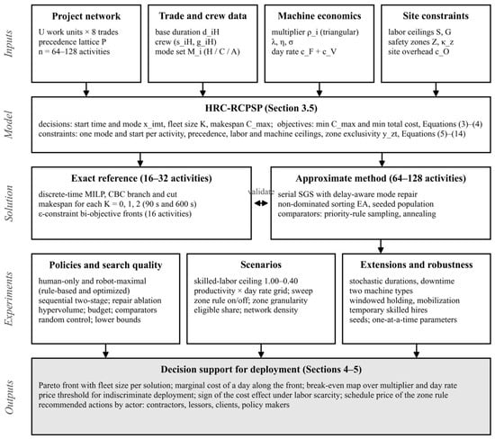
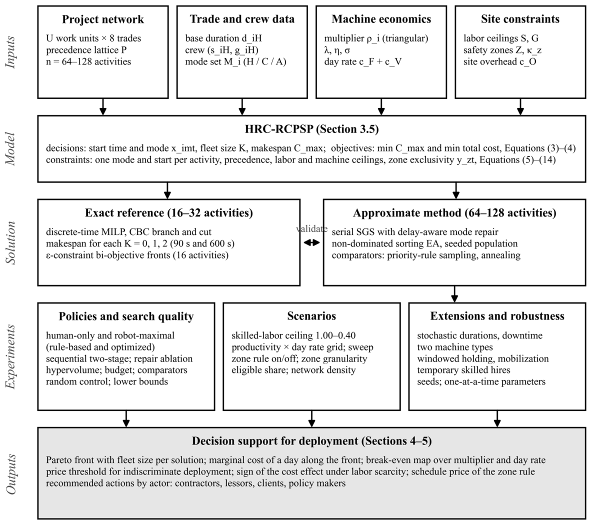
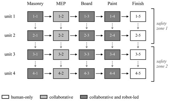
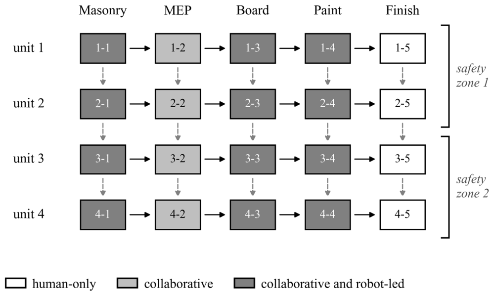
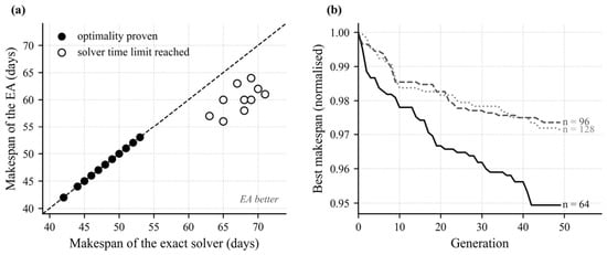
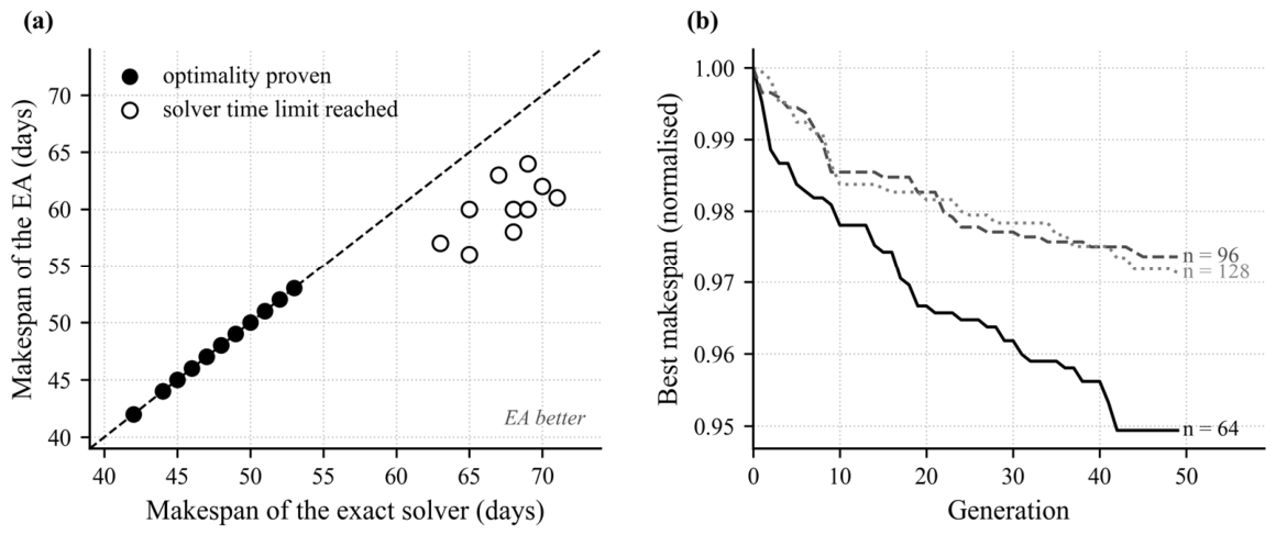
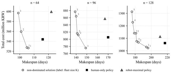
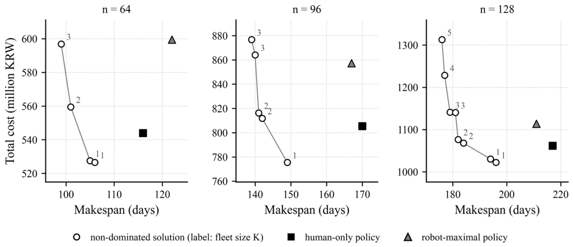
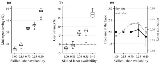
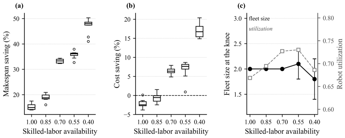
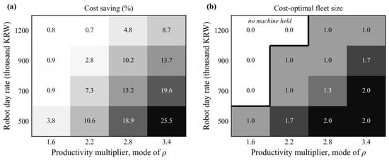
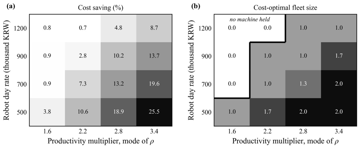
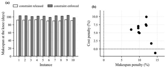
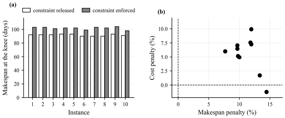
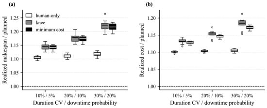
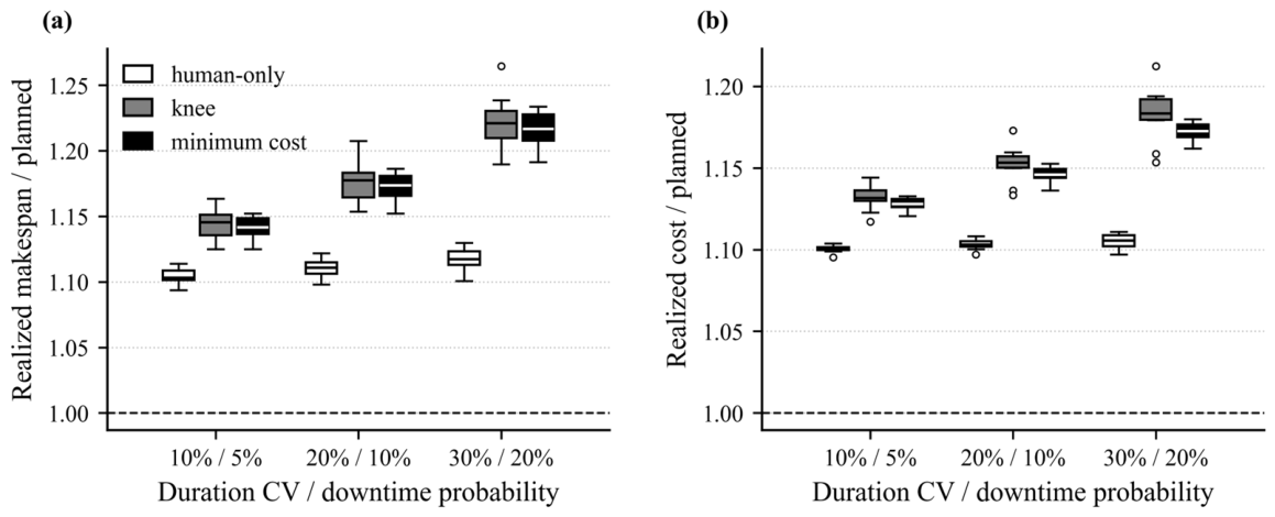
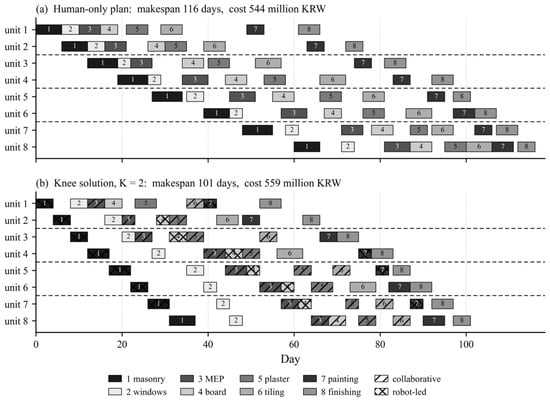
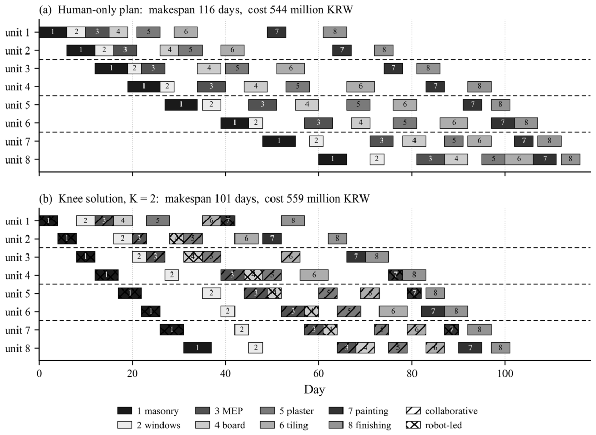

Disclaimer/Publisher’s Note: The statements, opinions and data contained in all publications are solely those of the individual author(s) and contributor(s) and not of MDPI and/or the editor(s). MDPI and/or the editor(s) disclaim responsibility for any injury to people or property resulting from any ideas, methods, instructions or products referred to in the content. |
© 2026 by the authors. Licensee MDPI, Basel, Switzerland. This article is an open access article distributed under the terms and conditions of the Creative Commons Attribution (CC BY) license.