


Abstract
To address the limitations of traditional route choice models, including their dependence on manually constructed path sets, their difficulty in capturing nonlinear decision preferences, and their insufficient consideration of dynamic congestion factors, this paper proposes an urban vehicle route choice modeling method that integrates trajectory map matching with adversarial inverse reinforcement learning. First, based on taxi GPS (global positioning system) trajectories, the OSM (Open Street Map) road network, Amap real-time traffic conditions, and POI (point of interest) data, a multi-source feature set including road-segment attributes, dynamic congestion, built environment, and destination context is constructed. Second, STGM-Net is used to convert raw GPS point trajectories into road-segment sequences. Furthermore, the route choice process is modeled as a Markov decision process at the road-segment scale, and an AIRL model is constructed to learn the latent reward function from real trajectories. Finally, the SHAP (Shapley additive explanations) method is introduced to analyze the influence of different features on route choice behavior. Experimental results show that the proposed model outperforms traditional discrete choice models and imitation learning models in terms of path similarity, distribution fitting, and traffic-flow restoration. Dynamic congestion level and shortest-path distance are key factors influencing vehicle route choice.
1. Introduction
With the continuous advancement of urbanization and the rapid growth of motor-vehicle ownership, urban road traffic systems are facing increasing operational pressure. The sustained growth of travel demand, the growing complexity of road-network structures, and the highly dynamic variation of traffic states have made traffic congestion, declining travel efficiency, and increasing transport energy consumption increasingly prominent. As an important component of travel decision-making, route choice behavior directly affects individual travel time, road traffic-flow distribution, and road-network operating conditions, and it constitutes an important basis for traffic assignment, congestion evolution analysis, and intelligent traffic management and control. Therefore, accurately characterizing urban vehicle route choice behavior is of great significance for revealing the travel decision-making mechanisms of traffic participants, optimizing traffic guidance strategies, and improving the operating efficiency of the transportation system [1,2].
Traditional route choice models are mostly based on random utility theory, with discrete choice models as the main representatives [3]. These models describe travelers’ choice probabilities among different routes by constructing candidate path sets and specifying path utility functions [4]. Such methods have been widely applied in transport planning and demand analysis, but they still have certain limitations under complex urban road-network conditions [5]. On the one hand, the number of feasible paths in a real road network is enormous, and it is difficult to exhaustively enumerate the complete path set; the results of candidate path generation can therefore easily affect model-estimation accuracy [6]. On the other hand, different paths often share many overlapping road segments, and path utilities exhibit obvious spatial correlation, which traditional discrete choice models have difficulty eliminating sufficiently. In addition, the form of the utility function usually depends on manual specification, making it difficult to accurately express travelers’ nonlinear decision preferences in dynamic traffic environments [7,8,9].
With the development of onboard positioning devices, mobile Internet, and connected-vehicle technologies, large-scale GPS trajectory data provide a new data foundation for route choice research [10]. Route choice modeling based on trajectory data can extract decision rules from real travel behavior, thereby improving the practical applicability of models [11]. At the same time, data-driven methods such as deep learning and reinforcement learning show strong advantages in high-dimensional feature representation, nonlinear relationship modeling, and sequential decision learning, and they have gradually been applied to route choice behavior modeling. Related studies have begun to regard the route choice process as a continuous decision process in which vehicles move forward segment by segment in the road network [12,13,14,15,16]. Segment-based modeling avoids the traditional problem of enumerating candidate paths and uses neural networks to enhance the model’s ability to represent complex traffic features [17,18].
However, existing deep-learning-based route choice models still face the problem of insufficient behavioral interpretability [19,20]. Although some end-to-end models can improve route prediction accuracy, their internal decision mechanisms are difficult to interpret, making it hard to reveal the specific effects of road attributes, traffic states, and environmental factors on route choice behavior [21,22,23,24]. In contrast, inverse reinforcement learning can infer travelers’ latent reward functions from observed real trajectories and learn their implicit preferences without prespecifying the form of the utility function, thus providing a new perspective for route choice modeling [25,26,27]. In particular, adversarial inverse reinforcement learning can simultaneously achieve route policy learning and reward-function estimation through adversarial training between a generator and a discriminator [28], and therefore has strong potential for characterizing complex route choice behavior [29,30,31,32,33].
Nevertheless, existing route choice studies based on inverse reinforcement learning still have the following shortcomings [24]. First, most studies focus on static road-network attributes such as road length and road class, while insufficiently considering dynamic traffic-environment factors such as real-time congestion, making it difficult to reflect the influence of changes in traffic operating conditions on route choice behavior [3]. Second, some models insufficiently characterize goal-oriented features such as destination direction and distance to destination, which may lead to deviations between generated routes and real travel routes in local decisions. Third, although deep inverse reinforcement learning models can improve path-fitting ability, the nonlinear reward functions they learn still have certain black-box characteristics, and the influence of different features on route choice decisions needs to be further explained. In addition, during trajectory data processing, GPS trajectories in complex urban environments are easily affected by signal drift, uneven sampling intervals, and dense road intersections [26]. If map-matching accuracy is insufficient, the training quality and reliability of subsequent route choice models will be directly affected [34,35,36,37].
To address these issues, this paper takes urban vehicle route choice behavior as the research object and constructs a multi-source data system integrating static road attributes, dynamic congestion states, built-environment features, and destination-context features based on taxi GPS trajectories [38,39], the OSM road network [40,41], Amap real-time traffic conditions [42], and POI data. In the trajectory processing stage, a multi-scale spatiotemporal graph-constrained map-matching method is adopted to convert raw GPS point trajectories into road-segment-level trajectory sequences [31,32,33]. In the route choice modeling stage, the vehicle route choice process is abstracted as a segment-based Markov decision process, and an adversarial inverse reinforcement learning route choice model considering dynamic congestion features is constructed to learn travelers’ latent reward functions from real trajectories. Furthermore, the SHAP method [35] is introduced to conduct feature attribution analysis of the reward function, revealing the influence mechanisms of different traffic-environment factors on vehicle route choice behavior.
The main contributions of this paper are as follows:
- (1)
- A route choice feature system integrating multi-source traffic-environment information is constructed. By integrating taxi GPS trajectories, the road network, real-time congestion, and POI data, vehicle route choice contexts are characterized from multiple dimensions, including static road-segment attributes, dynamic traffic states, built environment, and destination context, thereby improving the data representation capability for route choice behavior modeling.
- (2)
- An adversarial inverse reinforcement learning route choice model considering dynamic congestion features is proposed. The vehicle route choice process is modeled as a sequential decision-making problem at the road-segment scale, and the latent reward function is inferred from real trajectories through adversarial inverse reinforcement learning, avoiding the dependence of traditional models on manually specified utility functions and candidate path sets.
- (3)
- An interpretability analysis method is introduced to reveal the mechanisms influencing route choice. The SHAP method is used to analyze the feature contributions of the learned nonlinear reward function, quantifying the effects of road conditions, dynamic congestion, and environmental features on route choice behavior, and providing behavioral-mechanism references for urban traffic guidance and congestion management.
2. Dataset Construction and Feature Extraction
This paper takes taxi GPS trajectories in Wuxi as the main research object and combines the OSM road network, Amap real-time traffic conditions, and POI data to construct a dataset for route choice modeling. Taxi GPS data are used to identify actual vehicle trips and trajectory sequences; OSM road-network data are used to construct a passable road topology; real-time traffic-condition data are used to extract dynamic congestion states at the road-segment level; and POI data are used to characterize the built environment and functional attributes around roads [11,20,24].
The background city of this study is Wuxi, Jiangsu Province, located between 31°07′ and 32°00′ N and between 119°31′ and 120°36′ E. Figure 1 shows the location of Wuxi. The data involved in this paper cover the entire administrative area of Wuxi. In the data analysis stage, the urban area of Wuxi is selected, mainly Liangxi District, while also covering parts of Xishan District, Binhu District, Xinwu District, and Huishan District. The study area is approximately 64 square kilometers.
Figure 1.
The location of Wuxi.
The research data consist of GPS trajectory data collected from taxis operating in Wuxi. The data span a period of 31 days, from 18 July 2020 to 17 August 2020, including 21 weekdays and 10 non-weekdays, which adequately reflect the operational characteristics of taxis across different temporal periods. During this period, taxi operations, commuting, and general travel demand had essentially recovered after the outbreak of COVID-19, and no strict mobility restrictions were in place. Therefore, the influence of the pandemic on the travel patterns captured in this dataset is limited. The trajectory data were automatically collected via onboard terminals, with an average sampling interval of approximately 4–5 s. However, due to variations in communication environments and device conditions, trajectory points exhibit uneven sampling intervals.
Each individual GPS trajectory record primarily includes fields such as vehicle identification, spatial location, temporal information, and vehicle operational status. Specifically, the recorded fields comprise vehicle ID, longitude, latitude, collection time, heading direction, speed, longitudinal acceleration, lateral acceleration, vertical acceleration, and yaw rate. Among these, the longitude, latitude, and collection time fields are used to characterize the spatiotemporal position changes of the vehicle, while the remaining fields are employed to describe the vehicle’s operational status. The vehicle identification, spatial location, and temporal information serve as the primary fields for trajectory extraction, whereas the various acceleration measures and yaw rate are treated as auxiliary information.
Written data-use authorization was obtained from the Wuxi Connected Vehicle Group before the data were released to the study team. The data provider de-identified all records prior to transfer, and the research team received only anonymized data without any direct identifiers. Therefore, formal ethical approval was waived.
To ensure trajectory data quality, GPS points were first processed by removing outliers, sorting by time, checking speed rationality, and segmenting trajectories. Then, combined with road-network topology, the raw point trajectories were converted into road-segment-level trajectory sequences. Road-network preprocessing included road-type filtering, coordinate-system unification, road-topology construction, and road-segment attribute extraction. Finally, a route choice modeling dataset was constructed, in which road segments served as the basic analytical units and OD trips constituted the samples. More than 183,000 raw data were collected within the urban area of Wuxi city, and after processing, there were a total of 25,563 road trajectory sequences in the expert trajectory dataset [38,39,40,41,42].
Vehicle route choice is influenced not only by static attributes such as segment length and road class, but also by dynamic constraints such as real-time traffic states and destination direction. This paper constructs state features from four aspects [3,8,24,26,27].
- (1)
- Static road-network attributes. These include road-segment length, road class, road direction, topological connectivity, node degree, and relative distance to the destination, which are used to describe the travel conditions of the segment itself and its structural position in the road network.
- (2)
- Dynamic congestion features. Real-time traffic-condition data are used to classify road-segment traffic operating states, forming road-segment-level congestion-level features that characterize the dynamic traffic environment faced by vehicles at different times.
- (3)
- Built-environment features. Land-use functions are reclassified based on POI types, and the number, density, and functional-mix characteristics of different types of POIs within a certain buffer around each road segment are calculated to describe the activity environment along the road.
- (4)
- Destination-context features. Indicators such as the distance between the current segment and the destination, the direction angle, and the remaining-path trend are constructed to express goal orientation in the route choice process.
Together, these features constitute the state input of the route choice model, enabling the model to perceive road-network structure, real-time traffic states, and goal-oriented information simultaneously.
Due to the high cost of obtaining high-precision and true-labeled vehicle trajectory data, this paper proposes a simulation trajectory generation scheme based on road network topology structure, which provides large-scale and robust supervised learning samples for the training of STGM Net model.
Firstly, in the directed graph of the road network within the research scope, a pair of starting nodes O and ending nodes D are selected through uniform random distribution to ensure sufficient topological distance between the starting points to cover a variety of road types. As a benchmark for path generation, Dijkstra’s algorithm is used to search for the global optimal path between point O and point D on the road network. And define the weight cost coefficient of the algorithm as the physical length of the road segment. In order to make the generated simulation trajectory closer to the real distribution and enhance the generalization ability of the model, before performing path search, random error weights are injected into the original cost of each edge in the road network to generate the perturbed road segment cost :
where is the disturbance intensity coefficient, with a value of 0.1, and is a random variable that follows a standard normal distribution.
Through multiple iterations of the aforementioned perturbation process, multiple candidate path sets can be generated for the same pair of OD nodes that differ in spatial topology but are logically reasonable, and each path is composed of a series of ordered road segment indices , where the road segment index is the true label of the path.
After obtaining a topologically continuous sequence of real road segments, it is necessary to simulate the motion process of vehicles on the path and discretize it into a GPS trajectory point sequence with time attributes. A sampling frequency of and a sampling time interval of are assumed. For each time step on the path , the cumulative distance traveled by the vehicle on the road segment can be expressed as:
When the vehicle passes through the junction of the road section, it triggers a random stop behavior with a stop probability and a waiting time that follows a uniform distribution within the interval . Based on the calculated cumulative distance , the vehicle trajectory point is mapped to the geographic coordinate of the road section center line using a linear interpolation algorithm.
Real GPS coordinates often deviate from their true positions. In order to train the model’s correction ability in complex environments, this paper injects noise into the ideal sampling point sequence to simulate the spatial position drift, sampling sparsity, and outliers of GPS trajectory points. Using a Gaussian noise model to simulate spatial position drift, for each ideal trajectory point , inject independent latitude and longitude offsets to generate observation point :
where the standard deviation of determines the intensity of noise, and the range of values is meters.
Randomly discard some sampling points and simulate unstable sampling frequency caused by network latency or device power failure. Introduce large random jump points in the trajectory with probability to simulate the outlier phenomenon caused by signal reflection.
The final generated dataset structure has an input sequence of , consisting of a series of trajectory points containing latitude, longitude, time, and instantaneous velocity. The label sequence consists of a series of road segment IDs.
3. Models and Methods
3.1. STGM-Net Trajectory Map-Matching Method
GPS trajectory data are prone to drift, missing values, and noise in environments such as urban high-rise areas, tunnels, and complex intersections. Directly using such data for route choice modeling can distort road-segment sequences. To improve the quality of expert trajectories, this paper adopts STGM-Net to perform map matching on raw GPS trajectories [38,39,40,41,42].
STGM-Net adopts an encoder– decoder structure. The encoder consists of a multi-scale progressive temporal convolutional network and a GraphSAGE road-network embedding module [10,42]. The multi-scale progressive temporal convolutional network is used to extract short-term and long-term temporal dependencies in trajectory sequences, while GraphSAGE is used to learn structural representations of road-segment nodes in the road topology. The decoder adopts candidate subgraph constraints and a GRU (gated recurrent unit) sequence decoding mechanism to map GPS point sequences into road-segment sequences that conform to road-network topological connectivity [43].
The input of STGM-Net consists of a GPS trajectory point sequence and its candidate road-segment set, and the output is the matched road-segment sequence:
where denotes the matched road segment corresponding to the th time step. The model jointly learns spatial similarity constraints, topological connectivity constraints, and temporal features to improve matching robustness in complex road-network environments.
3.2. Markov Decision Process Modeling of Route Choice
The vehicle route choice process can be regarded as a sequential decision process in which the next road segment is selected step by step in the road network. This paper models it as a Markov decision process [13,14]:
where denotes the set of all states, denotes the set of all actions; is the state transition function, which determines the next state according to the current state and action to obtain the next state ; denotes the reward; and denotes the discount factor.
State Representation (): At each decision step , the state is a concatenated vector comprising (i) the current link ID, (ii) the remaining travel distance to the destination, (iii) the cumulative travel time incurred so far, (iv) the current time of day, and (v) a set of link-level attributes (free-flow speed, capacity, and historical congestion index) for the current link and its immediate successors. All continuous features are normalized to zero mean and unit variance using statistics computed from the training dataset.
Action Space (): The action is a discrete choice among the set of outgoing links from the current node, excluding the link that immediately led to the current node. The size of the action space varies per state, with a maximum out-degree of 8. Invalid actions are masked by setting their logits to before the softmax operation.
Transition Constraints (): The transition is deterministic and governed by the network topology: given action , the next state is obtained by advancing the agent to the downstream node of that link. The episode terminates when the agent reaches the destination node or when the number of steps exceeds a maximum horizon . No stochasticity is assumed in the transition dynamics.
3.3. Adversarial Inverse Reinforcement Learning Route Choice Model
Based on Markov decision process modeling, an Adversarial Inverse Reinforcement Learning (AIRL) framework is introduced to construct the route choice model [37,38,39,40,41,42].
As shown in Figure 2, the model framework consists of a data and environment layer, an adversarial reinforcement learning modeling layer, and an output application layer, forming a complete process from data input, feature representation, and adversarial learning to result output. Through the generator-discriminator adversarial mechanism, the road-segment sequences generated by the policy network gradually approximate the expert trajectory distribution, while the reward function that can explain expert route choice behavior is inferred, thereby achieving joint modeling of route choice policy and decision preferences [30,31,32,33].
Figure 2.
Framework of the adversarial deep inverse reinforcement learning model.
The data and environment layer mainly provides the road-network environment and expert samples. Based on the OSM road network, the topology is constructed, road-segment reachability relationships and state-transition constraints are extracted, and features such as the built environment, destination information, and dynamic congestion levels are integrated to characterize the route choice environment under complex traffic conditions. The training samples consist of expert trajectory road-segment sequences obtained after map matching. It should be clearly noted that this expert dataset has been pre-processed offline through the STGM-Net map-matching step. Only the matched road-network coordinates, rather than the raw noisy GPS points, are subsequently fed into the AIRL loop. The current segment, time, and destination are defined as the state, and the transition to a downstream adjacent segment is defined as the action, thereby converting the route choice process into a sequential decision problem in the road network [24,26,27].
In the adversarial reinforcement learning modeling layer, the generator’s policy network outputs action selection probabilities based on state features and interacts with the road-network environment to generate complete routes. The discriminator’s reward network judges the source of samples based on state-action pairs and learns reward signals that can explain expert behavior. After adversarial training converges, the optimal policy can output the probability of choosing the next segment under a given state, enabling segment-level route prediction and route generation. The learned reward function is used to characterize travelers’ comprehensive route choice preferences under the joint effects of road attributes, environmental features, and congestion states [31,32,33].
In the local action space , a feasibility mask vector is constructed for the action in the training sample. As shown in Figure 3, for the current road segment , 8 potential movement directions are checked. Feasible directions are marked as 0, and infeasible directions are marked as [43].
Figure 3.
Attention masking mechanism.
After the raw attention scores are computed, the mask matrix is added to the scores. is the original score vector.
If direction is feasible, ; if direction is infeasible, . The masked scores are then normalized using softmax to obtain the final attention weights ,
To accommodate the structural heterogeneity of real-world urban intersections—which commonly feature 3-way (T-junctions), 4-way (crossings), or 5-way junctions, as opposed to a fixed maximum of 8 directions—our method implements a dynamic action masking mechanism within the attention-based policy head.
While the neural network’s output layer is architecturally fixed to a maximum action dimension of A = 8, the physical validity of these actions is not uniform across all scenarios. To prevent the agent from selecting physically non-existent outbound links, we apply a hard attention mask to the action logits prior to the final softmax normalization.
This mask is constructed as follows:
Mask Generation: For each intersection, a binary validity vector is computed in real-time based on the current topological map. Entries corresponding to physically available outbound branches are set to 1; all other entries are set to 0.
Logit Injection: This validity vector is transformed into an additive mask by mapping and . This mask is then added element-wise to the raw action logit produced by the network’s final linear layer:
Softmax Invariance and Validity: The standard softmax function is then applied to the masked logit :
Because , the probability mass for all invalid actions is forced to exactly zero. Crucially, the softmax denominator automatically sums only over the valid, unmasked logits, guaranteeing that the probability distribution over the remaining actions sums to 1.
This approach yields two critical advantages:
Dynamic Elasticity: The network seamlessly adapts to -way junctions without requiring any architectural changes or retraining. The effective action space shrinks from 8 to on the fly.
Gradient Preservation: By applying the mask additively to the logits (rather than post hoc renormalization), we ensure that the policy gradient flows only through the valid action heads. The invalid heads contribute zero gradient, preventing the network from wasting capacity on impossible maneuvers while maintaining the theoretical guarantee that
Through the masking mechanism, only directions allowed by the road-network topology have positive probabilities in the action probability distribution output by the generator. This prevents trajectories that violate road-network topological rules and ensures that generated routes are physically connected in reality [43].
As shown in Figure 4, the generator model structure mainly consists of three parts: a feature embedding layer, a local context extraction module based on the attention mechanism, and a policy output layer. The feature embedding layer receives road-segment features, congestion-level features, contextual environment features, and built-environment feature vectors around the road segment.
Figure 4.
Generator model structure.
First, the feature-attention module recalibrates the importance of the input raw feature vector . To ensure the stability of adversarial generation and prevent gradient vanishing, the module uses the Sigmoid activation function to compute the weight of each feature dimension and adds the weighted features to the original feature vector through a residual connection, generating an enhanced feature representation. Second, the spatial-attention module introduces an attention mechanism to capture the influence of adjacent road segments in the road-network topology on the current decision. The hidden-layer feature vector is passed through a subnet consisting of a fully connected layer, an ReLU activation function, a masking layer, and a softmax normalization layer to calculate the association between the current segment and candidate segments and obtain spatial attention weights . Specifically, the masking layer masks unreachable connections according to the road-network topology. The weights are used to perform a weighted sum over the candidate road-segment feature vector set, generating a context vector that represents local environmental information. The model concatenates the current road-segment vector with the generated local environmental context vector, so that it focuses on current segment attributes while fully perceiving the traffic state of the surrounding road network. The policy output layer takes the fused comprehensive features as input and passes them through fully connected, masking, and softmax layers. After infeasible real-world segments are masked by the masking mechanism, the final output is a probability distribution over 8 movement-direction actions .
Generator Update: The policy is updated via proximal policy optimization (PPO) to maximize the expected cumulative reward from the discriminator. The objective is:
where
and is the generalized advantage estimation (GAE). An entropy bonus with coefficient c = 0.01 is added to encourage exploration. We performed 10 PPO epochs per AIRL iteration with a batch size of 64.
Update Schedule: At each iteration, (i) collect = 8916 trajectories using the current policy; (ii) update the discriminator 1 time; (iii) recompute rewards using the updated discriminator; and (iv) update the policy and value network with 10 PPO epochs. Training terminates upon policy entropy saturation, discriminator accuracy convergence, or reaching 500 iterations.
Training proceeds for a maximum of 500 AIRL iterations. We adopted two convergence criteria: policy entropy stability, where training is stopped when the rolling average (window size = 20) of the policy’s action entropy falls below 0.5 nats, indicating near-deterministic behavior; and discriminator accuracy saturation, where training is terminated if the discriminator accuracy on a held-out validation set remains within ±2% of 0.5 for 30 consecutive iterations, suggesting that the generated trajectories are indistinguishable from expert ones. If neither criterion is met, training terminates at 500 iterations.
As shown in Figure 5, the discriminator model structure first extracts road-segment features and congestion-level features as well as destination-context features to construct the initial local-environment context feature vector , and introduces an attention mechanism into the discriminator as well to capture the influence of different neighboring segments in the road network on the current decision. The discriminator’s core task is to recover the latent reward function , and to distinguish expert trajectories from trajectories generated by the generator through adversarial learning. The model adopts a structure based on the advantage function and decomposes it into a state–action reward term and a state–value shaping term .
Figure 5.
Discriminator model structure.
The AIRL training proceeds via an adversarial alternating optimization between the generator and the discriminator. Reward Function: The reward for a state–action pair is modeled as a neural network.
where is a 3-layer feedforward network with 128 hidden units and ReLU activations. The term serves as a policy entropy regularizer, ensuring that the recovered reward is invariant to the policy’s action distribution.
Discriminator Update: The discriminator is trained to distinguish expert trajectories from generated ones by minimizing the binary cross-entropy loss:
We perform 1 discriminator gradient step per generator update. After the update, the reward is derived as:
Reward Update: After updating the discriminator, the reward function is implicitly updated:
This reward is then used for the subsequent policy update.
The attention embedding layer uses an attention mechanism to dynamically process the features of the current road segment and its next candidate road segment. The current road segment and all locally reachable candidate road segments are mapped into a feature sequence, where each element contains the road segment’s static attribute features, relative relationship to the destination, and sliced features of the dynamic traffic congestion level. The state– action reward network estimates the instantaneous utility of executing a certain action in a specific context, and concatenates the local-environment context vector output by the attention embedding layer with the current action vector. Through a multilayer feedforward neural network, the fused features are mapped to a reward value. The state–value shaping term takes the current state and the state after executing the action as inputs to the multilayer feedforward neural network, and the features are input to the multilayer feedforward neural network, and it outputs the latent value of the state.
Following the Adversarial Inverse Reinforcement Learning (AIRL) framework proposed by Fu et al. [31], the discriminator is structured to distinguish between expert demonstrations and trajectories generated by the learned policy. The discriminator is defined as:
where the function decomposes into a reward approximator and a shaping term:
Combining the two equations yields the explicit linking relationship between the discriminator and the reward function:
This equation is the core of the AIRL framework. Its key contribution is that, by introducing the shaping function (a potential function), the learned reward (s,a) is disentangled from the environment dynamics . Specifically, the presence of ensures that when the environment transition dynamics change, the optimal discriminator still recovers the same reward function (up to a constant), thereby endowing the learned reward with cross-environment transferability.
All symbols are explicitly defined as follows:
—AIRL discriminator output, representing the probability that the current state–action–next-state tuple comes from expert demonstrations;
—Reward approximator (parameterized by ϕ), which serves as the final extracted reward function ;
—Shaping/potential function (parameterized by ), which disentangles the reward from environment dynamics;
—Discount factor of the Markov decision process;
—Current policy (parameterized by ).
This fundamental linking equation directly reflects the key innovation that distinguishes AIRL from other IRL methods: through the coupled design of the discriminator and the policy, together with the shaping term , the reward recovery process is rendered independent of specific environment transition dynamics, thus enabling reward transferability.
3.4. PPO-Based Policy Optimization
In the adversarial inverse reinforcement learning framework, the generator’s policy network needs to be continuously optimized to generate route trajectories that approximate real driving behavior. Traditional REINFORCE policy gradient methods are prone to unstable or even collapsed training because an excessive step size can lead to drastic policy updates. Therefore, this study uses the proximal policy optimization (PPO) algorithm to train the generator. PPO is a deep reinforcement learning algorithm based on an actor–critic [44] architecture with model-free [45], online [46], and on-policy [47] attributes. PPO limits the magnitude of policy updates by introducing a clipping mechanism, thereby significantly improving convergence stability while ensuring sample efficiency.
Table 1 presents the pseudocode of the PPO algorithm. The specific procedure is as follows:
Table 1.
PPO algorithm procedure.
4. Experimental Design
4.1. STGM-Net Trajectory Map-Matching Model
During model training, the core optimization objective of the network is to minimize the distributional difference between the predicted road segment and the true label. Since map matching is essentially a multiclass classification problem, that is, predicting the best-matched road-segment class from the candidate segment set for each trajectory point. This paper adopts cross-entropy loss as the objective function for model training. Specifically, given the point-level true road-segment label sequence and the output path predicted by the model , the cross-entropy loss function is defined as follows:
where is the length of the input trajectory sequence; C it is the total number of candidate road-segment classes in the target space; is the indicator function, which equals th trajectory point’s true physical matched road segment is 1 and otherwise equals 0; is the predicted probability that the th trajectory point is mapped to a road segment by the decoder.
The structural parameters of the STGM-Net model are shown in Table 2, mainly covering three modules: the PD-TCN trajectory encoder, the GraphSAGE road-network encoder, and the gated GRU decoder.
Table 2.
Hyperparameter settings of STGM-Net modules.
In PD-TCN, the input feature vector dimension corresponds to the four-dimensional feature representation of trajectory points in Formula. . The dilation rates of the three dilated convolution layers are set to [1, 2, 4], corresponding to the short, medium, and long temporal scales. This expands the receptive field to 13 time steps without increasing the number of parameters. PD-TCN output dimension is kept consistent with GraphSAGE output dimension to support cosine-similarity attention calculation in the decoder.
The initial GraphSAGE road-segment feature dimension is set to 8, including the normalized coordinates of the two endpoints of the segment, segment length, sine and cosine of the azimuth angle, and the road-class code extracted from attribute fields and normalized to the [0, 1] interval. The number of graph convolution layers aggregates 2-hop topological neighborhood information for each road segment. The gated GRU decoder’s hidden-state dimension is aligned with the encoder output dimension and set to 128.
The training strategy hyperparameters of the model are shown in Table 3. The optimizer is Adam, the learning rate is set to , and the training, test, and validation sets are divided at a ratio of 8:1:1 at the trajectory level. And the 8:1:1 trajectory-level split is used only for the final held-out test set. The five-fold time-series cross-validation is applied exclusively to the 80% training portion for hyperparameter tuning and model selection.
Table 3.
List of model training hyperparameters.
We employed a grid search combined with 5-fold time-series cross-validation for hyperparameter tuning. To prevent data leakage, all cross-validation splits were performed strictly in chronological order, ensuring that validation sets do not contain future information.
Search Ranges (key hyperparameters as examples): Learning rate: {1 × 10⁻⁴, 5 × 10⁻⁴, 1 × 10⁻³}; Batch size: {64, 128, 256}; Hidden dimension: {64, 128, 256}; Discriminator update steps: fixed at 1 (corrected per previous comment); Behavior cloning (BC) loss weight λ: {0.1, 0.5, 1.0, 2.0}; Gradient penalty (GP) coefficient: {1.0, 5.0, 10.0}.
Selection Criterion: We used the average validation return as the primary selection metric, supplemented by the policy success rate as a secondary metric to balance performance and stability. The final hyperparameter configuration selected was the one achieving the highest average validation return.
Validation Procedure: For each fold of cross-validation, the model was trained for full iterations and evaluated on the validation set every 5 iterations (each evaluation averaged over 10 random seeds). The final hyperparameters were selected based on the best average performance across all 5 folds.
We place high importance on fair baseline comparisons and have taken the following measures:
Unified Tuning Protocol: All baseline methods (including BC, DAgger, GIRL, AIRL, etc.) were tuned using exactly the same search ranges, cross-validation procedure, and evaluation protocol as our method. Each baseline underwent independent grid search within its own search space, and its optimal configuration was selected based on its own validation performance.
Computational Budget Consistency: All baselines were trained using the same hardware resources and the same set of random seeds as our method.
To comprehensively evaluate the matching performance of the STGM-Net model, this paper draws on evaluation methods from sequence-to-sequence learning and machine translation and adopts three indicators, namely AHD, F-score, and BLEU score, for quantitative evaluation from both point-level matching and segment-level matching perspectives. On the one hand, point-level matching focuses on whether each GPS trajectory point can be accurately mapped to its corresponding real road segment. On the other hand, segment-level matching reflects the matching degree of the connected road-segment sequence of the vehicle’s real global trajectory.
In information theory, average hamming distance (AHD) is used to measure the number of symbols that differ at corresponding positions between two equal-length strings. In the evaluation of the map-matching model, it is converted into an indicator for calculating model matching accuracy:
where denotes the total number of trajectory points or road segments correctly matched by the model to the true label, denotes the total number of input trajectory points or road segments. The closer the indicator value is to 1, the higher the spatial mapping accuracy of the model.
The F-score is one of the most commonly used indicators for measuring the prediction accuracy of binary or multi-class classification models. In complex road-network matching scenarios, a single precision or recall measure is often insufficient to fully reflect the true performance of a model. Therefore, the F-score introduces the harmonic mean of precision and recall to evaluate matching accuracy:
denotes the proportion of road segments predicted as correctly matched that actually belong to the real vehicle trajectory path; denotes the proportion of all actually traveled road segments that are successfully predicted and correctly matched by the model. F-score ranges from [0, 1], and the closer its value is to 1, the better the model balances suppressing mismatches and reducing missed matches, and the stronger its overall matching performance.
BLEU was originally an evaluation metric commonly used in machine translation and Seq2Seq sequence generation. In map matching, compared with evaluating a single trajectory point in isolation, BLEU can scan the matching of consecutive trajectory points in the output sequence to effectively evaluate the order of trajectory-segment combinations and the completeness of the global path. To prevent the model from obtaining an artificially high score by repeatedly generating the same high-frequency segment, BLEU introduces a clipped modified precision ,
where denotes the number of elements contained in the currently counted continuous segment block; is the set of all unique segment blocks in the model output sequence; is the actual frequency of block in the model output sequence; denotes the maximum frequency of block in the corresponding true reference sequence; and is the total number of blocks contained in the model output sequence.
In addition, because shorter candidate sequences are usually prone to abnormally high precision, BLEU further introduces a brevity penalty factor to limit short-sighted behavior caused by overly short generation. The final score is jointly determined by the geometric mean of the first orders of modified precision and the brevity penalty factor,
where represents the length of the predicted sequence generated by the model, and represents the reference path sequence length closest to the length of the predicted sequence.
To evaluate the matching performance of the proposed STGM-Net model, this section selects three representative classical algorithms and frontier deep-learning models in the field of map matching as baseline models for comparative analysis [38,39,40,41,42].
- (1)
- The FMM (Fast Map-Matching) algorithm is an efficient and highly scalable fast map-matching algorithm. Based on the hidden Markov model, it introduces a precomputation mechanism by preconstructing an origin–destination table containing shortest paths and using fast hash-table search instead of repeated path-query operations, thereby greatly improving matching efficiency when processing large-scale trajectory data [40].
- (2)
- The ST-Matching model is a classical map-matching algorithm for low-sampling-rate GPS trajectories. Its core idea is to construct a candidate road-segment graph by comprehensively considering the spatial geometric features of the road network, topological connectivity, and temporal attributes of trajectories, and then to search this graph to identify the best matched path [38,39].
- (3)
- BiLSTM–Attention model: This model uses a bidirectional long short-term memory network (BiLSTM) to extract bidirectional temporal features of GPS trajectories and introduces an attention mechanism to perform weighted aggregation of trajectory features at different time steps so as to capture key movement states. As a representative deep sequence learning model, it can better cope with trajectory-noise interference. However, because its road-segment representation mainly relies on learnable embedding vectors and lacks explicit road-network topological constraints, it has certain limitations in judging logical connectivity in complex road-network environments.
The performance of STGM-Net and the baseline models on the Wuxi taxi test set is shown in Table 4:
Table 4.
Comparison of model performance.
STGM-Net achieves the best performance on the Wuxi taxi trajectory dataset, while FMM performs the worst, with an AHD of only 0.7213. The main reason is that it relies only on the projection distance from GPS points to road segments as the observation probability, which provides limited discrimination in areas with dense road segments. After introducing temporal consistency constraints, ST-Matching improves its AHD to 0.7658, but its path inference capability for low-sampling-rate trajectories remains limited. BiLSTM–Attention adopts sequence learning and can capture the temporal context of trajectories, but its road-segment representation is provided only by a learnable embedding table and lacks road-network topology priors, leading to mismatches in segment-connectivity judgment.
4.2. AIRL-Based Route Choice Model
To ensure the convergence stability and generation quality of the adversarial inverse reinforcement learning model when processing complex urban road networks, this study refers to the experimental settings in the related literature and conducts a series of hyperparameter tuning. The specific parameter settings are shown in Table 5 [31,32,33,44].
Table 5.
Hyperparameter settings for AIRL model training.
In terms of hardware environment, the experiments were run on a server equipped with an RTX 4090 GPU (24 GB memory), a 12-core Intel Xeon Platinum 8352 V@2.10 GHz CPU, and 90 GB RAM. The software environment was Python 3.9, the deep-learning framework was PyTorch 1.9.0, and the CUDA version was 11.1.
Table 6, Table 7 and Table 8 respectively list the experimental results of the AIRL-based route choice model used in this paper, the baseline PSL, DNN-PSL, and R-logit models, and two imitation learning models, BC and GIRL, under sample sizes of 100, 1000, and 10,000. The experimental results came from a single run [3,5,48].
Table 6.
Model training results with 100 samples.
Table 7.
Model training results with 1000 samples.
Table 8.
Model training results with 10,000 samples.
This article builds an evaluation index system from two dimensions: the generation capability of a single path and the overall accuracy of the model. Among them, ED (Edit Distance) and BLEU (Bilingual Evaluation Understudy) focus on the accuracy of individual path sequences, while JSD (Jensen–Shannon Distance) and LP (Log Probability) focus on the accuracy of the model’s overall statistical distribution.
Across all sample sizes, the AIRL model performs best on all four indicators. With only 100 samples, its ED is already as low as 0.28 and its BLEU reaches 0.65. With 10,000 samples, ED further decreases to 0.21 and BLEU increases to 0.72. Through the adversarial mechanism between the generator and discriminator, AIRL not only approximates real routes at the sequence level, but more importantly infers and learns the latent reward function. This grasp of the underlying decision logic gives it strong generalization ability under small-sample conditions and enables highly accurate route generation and probability-distribution restoration under large-sample conditions [7,8,9,48].
BC performs poorly with 100 samples, with ED as high as 0.47 and LP as high as 22.0. However, when the sample size reaches 10,000, all indicators improve substantially, with ED decreasing to 0.23 and BLEU reaching 0.72, numerically approaching AIRL. BC is essentially a supervised learning model that regards route choice as a direct mapping from states to actions. Under small-sample conditions, it is easily constrained by error accumulation in sequential decision-making. Under large-scale data training, however, it can achieve end-to-end replication by accurately capturing high-frequency statistical features in expert data. Nevertheless, it is only pattern matching and lacks an understanding of the underlying physical attributes of routes, making it prone to overfitting [30,49].
GIRL’s performance lies between that of AIRL and BC: it is clearly superior to BC under small-sample conditions, but not as good as AIRL and BC under large-sample conditions. GIRL fits occupancy measures from expert samples through a generative mechanism, giving it better generalization ability than BC. However, the high LP values indicate that although the trajectories generated by GIRL are similar to real route choices, the conditional transition probabilities computed by the model still deviate from the true decision logic.
Overall, the traditional comparison models are inferior to the three imitation learning models in training performance. Among them, R-logit simplifies decisions into a fixed combination of immediate rewards and lacks dynamic evaluation of global contextual information, making it difficult to precisely characterize complex preferences. The utility calculation of PSL depends heavily on pre-generated candidate path sets, and candidate-set generation algorithms often cannot effectively simulate humans’ real cognitive maps, leading to model bias. Although DNN-PSL introduces a multilayer perceptron to extract high-dimensional nonlinear features, its underlying framework is still constrained by the PSL structure that requires prespecified path sets. The complex features learned by the neural network may be transformed into model noise, preventing it from resolving the systematic bias caused by incomplete candidate sets [3,5,6,7,9].
5. Results and Analysis
5.1. Evolution of Feature Attention Weights Across Different Time Periods
To reveal the influence of each feature when the adversarial inverse reinforcement learning model simulates drivers’ route choices, the weight coefficients learned by the generator feature-embedding attention layer were extracted and visualized, as shown in Figure 6.
Figure 6.
Heat map of attention scores for feature categories.
Among them, contextual features maintain the highest weight level across all time periods, indicating that drivers rely heavily on current movement states and spatiotemporal correlation information when making route decisions. Congestion level and road-network attributes have the next highest weights, and the two show strong synergistic fluctuations. In contrast, built-environment features have the lowest weights, ranging from 0.18 to 0.22, and remain the most stable. This suggests that although static factors such as POI distribution provide a decision-making background, their direct driving effect on microscopic route choice is relatively limited.
From the perspective of dynamic evolution over time, the color of congestion-level features becomes significantly deeper and their weights increase markedly during the morning peak (8:00–9:30) and evening peak (17:00–19:30). This indicates that when traffic pressure increases, drivers’ decision logic actively shifts toward avoiding congested areas and pursuing travel efficiency. During the early-morning period (0:00–5:00) and the afternoon off-peak period, road-network attributes and contextual features dominate. This shows that under smooth traffic conditions, drivers are more inclined to follow established road-class preferences or habitual driving patterns when choosing routes.
5.2. SHAP-Based Attribution Analysis of Reward-Function Feature Contributions
The analysis based on the SHAP explanation framework shows that the vehicle route choice model exhibits a clear efficiency-first logic during decision-making, and feature influence presents a distinct gradient distribution. From the global feature importance in Figure 7a, shortest-path distance, congestion level, and the total number of road segments are the core factors determining route choice probability, among which shortest-path distance contributes far more than the other variables and plays a dominant role. For the taxi trajectory data used in this study, drivers are motivated by profit and are highly sensitive to fuel consumption (affected by distance) and time cost (affected by congestion). Second, road-network class and topological attributes (high-class road-segment count and straight-through proportion) have substantial effects on route choice, reflecting that drivers strongly rely on shortening physical distance and ensuring travel speed when selecting routes. In contrast, various land-use features (such as residential, commercial, and industrial land distribution) and POI indicators rank lower in importance, indicating that at the macro route-planning level, the social attributes of the surrounding environment make relatively weak marginal contributions to model decisions, while the model tends to capture the geometry and operating state of the road itself [34,35].
Figure 7.
SHAP value distribution of the discriminator reward network.
From the positive and negative effects of different features on the model in Figure 7b, the strong negative effect of congestion level reflects the instantaneous reduction of route attractiveness caused by dynamic urban traffic conditions. This negative feedback mechanism is converted into a relatively high penalty weight in the reinforcement learning model. In addition, the negative correlation of the total number of road segments can be attributed to traffic-signal delay risk: more segments imply higher intersection density, resulting in increased stop-and-go losses and safety risks. This is consistent with drivers’ preference for continuous routes with sparse nodes. For road-network class and topology, the positive contributions of high-class segment count and straight-through proportion essentially result from the higher design speeds and better driving stability of expressways or arterial roads, which can significantly reduce drivers’ psychological fatigue and operational complexity, forming a dual physical and psychological preference. In contrast, land-use and POI indicators have weaker influence on the route choice model because such features are usually spatially static attributes that mainly affect the generation of travel destinations. In a given O-D route choice process, road attributes such as speed and connectivity are more influential than static surrounding attributes [36,37].
5.3. Model Performance Analysis
The road-segment flow distribution aggregated over multiple OD pairs can reflect the model’s ability to learn global road-network travel preferences and its effect in assigning travel demand to the road network. This subsection aggregates microscopic individual route decision behavior at the macroscopic level and compares the consistency between the expected flow distributions generated by different models and the real flow distribution. In this experiment, 3000 actual trip origins and destinations are extracted from the Wuxi taxi trajectory data. Pretrained route choice models are used for path inference, and the inferred results are superimposed onto the road network to obtain estimated flows for each road segment [1,2,50,51,52].
This paper uses to quantify model goodness of fit, with a value range from 0 to 1. The closer the 1, the better the fitting effect of the model. Conversely, if approaches 0, it indicates that the model has difficulty capturing the intrinsic patterns in the data and has poor fitting performance.
Table 9 presents the comparative experimental results of different models in terms of goodness of fit . The experimental data show that the AIRL model performs best, with its reaching 0.915, significantly higher than those of the other comparison models. This indicates that the adversarial inverse reinforcement learning framework has strong representational ability in capturing the latent reward structure and nonlinear features of target behavior. Second, the BC model and the GIRL model also show high fitting levels, indicating that imitation-learning-based methods have good robustness on this dataset. In contrast, traditional discrete choice models perform weakly. The PSL model has the lowest value, while the DNN-PSL model with an introduced deep neural network shows only a slight improvement in goodness of fit.
Table 9.
Comparison of goodness of fit across models.
Figure 8 shows the road-segment flow distribution aggregated from real trajectories. The real road-network flow exhibits significant nonuniformity and skeletonized characteristics. A small number of core arterial roads and urban expressways carry most of the traffic load, appearing as dark-blue high-flow corridors in the figure, while many secondary and branch roads have low flows and appear light yellow or light green. This distribution objectively reflects the high spatial concentration of urban traffic flow.
Figure 8.
Actual road-segment flow distribution.
Comparing the experimental results of different models in Figure 9, it can be found that the models differ significantly in their ability to restore the road-network flow distribution. In Figure 9a, the AIRL model performs best; the locations and coverage of the high-flow segments it generates are most similar to the real distribution, restoring the concentrated flow distribution of ring-shaped and radial arterial areas in the core road-network region. The BC model ranks second. Although it can identify major traffic corridors, its local flow concentration is slightly weaker than that of AIRL, reflecting the limitations of behavioral cloning in handling long-sequence decision bias accumulation. The GIRL model can also generally represent the distribution structure of road-network flow, but its overall color is lighter, indicating insufficient estimation of the attraction of core segments. Traditional discrete choice models and their variants perform worse. The R-logit model produces an overly smooth flow distribution and cannot form an obvious high-flow backbone network. The PSL and PSL-DNN models perform the worst; the whole road network almost shows a uniform flow distribution, losing the spatial distribution characteristics of real traffic flow [3,6].
Figure 9.
Road-segment flow distributions of different models.
To complement the above experimental results, we further assessed the statistical reliability and uncertainty of the observed performance differences. All experiments were repeated five times with different random seeds (42, 1234, 5678, 91,011, and 2024) for each model, and we report the mean ± standard deviation of the values across these runs. For the AIRL model, we additionally computed 95% confidence intervals via bootstrap resampling (1000 iterations) to quantify estimation uncertainty.
The AIRL model achieves a mean of 0.915 ± 0.006, with the narrowest confidence interval among all methods, indicating high estimation precision and stable convergence behavior. The BC model yields 0.893 ± 0.009, and the GIRL model yields 0.897 ± 0.011, both exhibiting slightly larger variability. Traditional discrete choice models show considerably wider standard deviations, with the PSL model at 0.771 ± 0.014 and the PSL-DNN at 0.798 ± 0.013, reflecting greater sensitivity to initialization and optimization dynamics. The R-logit model achieves 0.832 ± 0.012; however, its estimated flow distribution is overly smooth and fails to form a pronounced high-flow backbone network, suggesting that the route choice logic embedded in the R-logit framework lacks the capacity to capture sharp structural asymmetries in the traffic assignment.
We also consider the practical meaningfulness of these improvements. In accordance with common practice in transportation modeling, and considering the inherent noise level in empirical traffic flow data, an absolute error gain of ≥0.03 or more is considered to represent a systematic improvement beyond random fluctuations, and is therefore of practical engineering significance. In transportation behavior studies, especially those using choice-based data with high inherent noise, values typically range between 0.3 and 0.7 at the disaggregate level. At the aggregate level, values are generally higher but marginal improvements tend to be smaller; thus, a 0.03 gain in at this level corresponds to a non-negligible reduction in prediction error, which can translate into measurable benefits in applications such as congestion forecasting and infrastructure planning. The AIRL model exceeds this threshold against all baselines, with a margin of +0.042 over BC and +0.173 over PSL. This suggests that the observed advantages are likely to translate into tangible benefits in real-world applications, such as more reliable congestion prediction and infrastructure planning.
In terms of the visual flow-restoration results shown in Figure 9, we note that the qualitative differences across models are consistent with the quantitative uncertainty analysis. Models with tighter confidence intervals and lower variability (e.g., AIRL) also produce spatially more coherent and stable flow patterns, whereas models with high uncertainty (e.g., PSL and PSL-DNN) tend to yield overly smoothed or uniform distributions. This consistency reinforces the interpretation that AIRL’s structural advantages—particularly its segment-based formulation and freedom from predefined candidate sets—contribute to both higher accuracy and greater robustness.
When comparing multiple models, a standard practice for consistent uncertainty reporting is to present the mean of the performance metric along with its variability measure, such as the standard error or a confidence interval.
The specific procedure is: obtain multiple estimates of the performance metric for each model through resampling techniques, then compute the standard deviation of these estimates as the standard error, which quantifies the uncertainty of the estimate. For visualization, error bars can represent standard errors, and shaded regions can represent confidence intervals.
The above results may be due to inherent defects in path-based models. Models based on complete paths need to sample potential paths to form a limited candidate set. Constrained by candidate-set generation algorithms, such models can allocate flow only to several pre-generated shortest paths, causing many suboptimal segments that are actually used to be completely ignored. In contrast to the PSL series models, AIRL is essentially a segment-based route choice model and has greater advantages in macroscopic traffic-flow assignment. It does not require a predefined choice set and can simulate candidate routes according to the learned policy, thereby covering a broader range of the real network [7,8].
6. Conclusions
This paper focuses on vehicle route choice behavior modeling in complex urban road networks and proposes a route choice modeling method that integrates multi-source traffic features with adversarial inverse reinforcement learning. The main conclusions are as follows:
- (1)
- Multi-source data fusion can improve the state representation capability of route choice. By integrating taxi GPS trajectories, the OSM road network, real-time congestion states, and POI data, vehicle route choice conditions can be characterized from multiple dimensions, including road-network structure, traffic operations, built environment, and destination orientation [11,20,24].
- (2)
- STGM-Net can effectively improve GPS trajectory map-matching accuracy. The model extracts trajectory temporal features through multi-scale temporal convolution, represents road-network topology using GraphSAGE, and introduces candidate subgraphs and topological constraints in the decoding stage. As a result, its matching results outperform comparison models in spatial accuracy, road-segment identification, and sequence similarity [38,40,41,42].
- (3)
- The AIRL model can better characterize the sequential decision mechanism of route choice. The model does not depend on manually specified utility functions or candidate path sets, but instead infers latent reward functions from real trajectories. Across different sample sizes, it shows good path similarity, distribution fitting ability, and generalization ability [19,21,24,25,27,28,30,33,49].
- (4)
- Dynamic congestion and shortest-path distance are key factors influencing route choice. SHAP interpretation results show that drivers’ route choices exhibit clear sensitivity to distance cost and a tendency to avoid congestion. Congestion level has a negative effect on route attractiveness, while POI built-environment features mainly serve as background influences and make relatively limited marginal contributions to microscopic segment-transfer decisions [24,26,34,37].
- (5)
- AIRL has good capability for reproducing aggregated traffic flows. Validation results across multiple OD pairs show that the road-segment flow distribution formed by AIRL-generated routes is closest to the real observations. This indicates that the model is suitable not only for individual route choice prediction, but also for supporting dynamic traffic assignment and route-guidance strategy evaluation [1,2,50,51,52].
In summary, the method proposed in this paper provides a technical path for urban vehicle route choice behavior modeling under dynamic traffic environments that combines data-driven capability, sequential decision representation, and behavioral interpretability. It can support personalized route guidance, traffic-flow prediction, and urban road-network optimization in intelligent transportation systems.
Several limitations of this study should be acknowledged.
- (1)
- Our analysis relies exclusively on taxi trajectory data, which may not fully represent the travel patterns of other population segments or transportation modes, potentially introducing selection bias.
- (2)
- The findings are context-dependent and may exhibit regional specificity, as traffic dynamics and road network characteristics are inherently tied to the study area; thus, generalizing these results to other cities or regions should be done with caution. We state that the framework is designed to be transferable—because it learns a reward function and a policy over generic network and behavioral features rather than hard-coded city-specific rules—but that empirical validation on external datasets remains future work.
- (3)
- Data privacy concerns impose constraints on data sharing and fine-grained spatiotemporal analysis, which may limit the reproducibility and extensibility of our approach.
- (4)
- The absence of external validation against independent ground-truth datasets leaves the accuracy of our inferred metrics unconfirmed.
- (5)
- The reliability of our results is contingent upon the precision of the map-matching algorithm and the quality of the underlying congestion data; any systematic errors or inherent inaccuracies in these inputs could propagate through our analytical pipeline and affect the robustness of our conclusions.
Author Contributions
Conceptualization, S.Z.; Methodology, S.Z.; Software, B.W.; Validation, C.Z.; Formal analysis, X.X.; Investigation, X.X.; Resources, G.M.; Data curation, G.M.; Writing—original draft, X.X.; Writing—review & editing, Y.L.; Visualization, B.W.; Supervision, G.M. All authors have read and agreed to the published version of the manuscript.
Funding
This work was supported by the National Natural Science Foundation of China (Grant No. 52572341).
Data Availability Statement
The original contributions presented in this study are included in the article. Further inquiries can be directed to the corresponding author.
Conflicts of Interest
The authors declare no conflicts of interest.
References
- Liu, G.; He, J.; Luo, Z.; Yao, X.; Fan, Q. Understanding route choice behaviors’ impact on traffic throughput in a dynamic transportation network. Chaos Solitons Fractals 2024, 181, 114605. [Google Scholar] [CrossRef] [Scilit]
- Han, X.; Sun, Q.; Xing, Y.; Gao, Z.Y.; Zhang, H.M. Reducing strategic uncertainty in transportation networks by personalized routing advice: A route-choice laboratory experiment. Travel Behav. Soc. 2024, 34, 100701. [Google Scholar] [CrossRef] [Scilit]
- Duncan, L.C.; Watling, D.P.; Connors, R.D.; Rasmussen, T.K.; Nielsen, O.A. Path Size Logit route choice models: Issues with current models, a new internally consistent approach, and parameter estimation on a large-scale network with GPS data. Transp. Res. Part B Methodol. 2020, 135, 1–40. [Google Scholar] [CrossRef] [Scilit]
- Shao, M.; Chen, C.; Feng, T. Scenic toll roads or cost-effective free roads? A stated preference analysis of private car users. Transp. Policy 2026, 179, 103983. [Google Scholar] [CrossRef] [Scilit]
- Prato, C.G. Route choice modeling: Past, present and future research directions. J. Choice Model. 2009, 2, 65–100. [Google Scholar] [CrossRef] [Scilit]
- Liu, D.J.; Li, D.W.; Gao, K.; Song, Y.; Zhang, T. Enhancing choice-set generation and route choice modeling with data- and knowledge-driven approach. Transp. Res. Part C-Emerg. Technol. 2024, 162, 104618. [Google Scholar] [CrossRef] [Scilit]
- Fosgerau, M.; Frejinger, E.; Karlstrom, A. A link based network route choice model with unrestricted choice set. Transp. Res. Part B-Methodol. 2013, 56, 70–80. [Google Scholar] [CrossRef] [Scilit]
- Mai, T.; Fosgerau, M.; Frejinger, E. A nested recursive logit model for route choice analysis. Transp. Res. Part B-Methodol. 2015, 75, 100–112. [Google Scholar] [CrossRef] [Scilit]
- Haj-Yahia, S.; Mansour, O.; Toledo, T. Incorporating domain knowledge in deep neural networks for discrete choice models. Transp. Res. Part C-Emerg. Technol. 2025, 171, 105014. [Google Scholar] [CrossRef] [Scilit]
- Qiu, S.H.; Qin, G.Y.; Wong, M.L.; Sun, J. RoutesFormer: A sequence-based route choice Transformer for efficient path inference from sparse trajectories. Transp. Res. Part C-Emerg. Technol. 2024, 162, 104552. [Google Scholar] [CrossRef] [Scilit]
- Wu, X.; Zhang, Z.; Wan, W. Travel route recommendation with a trajectory learning model. Complex Intell. Syst. 2024, 11, 12. [Google Scholar] [CrossRef] [Scilit]
- Mazzia, V.; Salvetti, F.; Aghi, D.; Chiaberge, M. DeepWay: A Deep Learning waypoint estimator for global path generation. Comput. Electron. Agric. 2021, 184, 106091. [Google Scholar] [CrossRef] [Scilit]
- Ke, Z.M.; Zou, Q.L.; Liu, J.C.; Qian, S. Real-time system optimal traffic routing under uncertainties—Can physics models boost reinforcement learning? Transp. Res. Part C-Emerg. Technol. 2025, 173, 105040. [Google Scholar] [CrossRef] [Scilit]
- Long, X.Q.; Mao, J.X.; Qiao, Z.B.; Li, P.; He, W. Reinforcement learning of route choice considering traveler’s preference. Transp. Lett.-Int. J. Transp. Res. 2024, 16, 658–671. [Google Scholar] [CrossRef] [Scilit]
- Low, E.S.; Ong, P.; Cheah, K.C. Solving the optimal path planning of a mobile robot using improved Q-learning. Robot. Auton. Syst. 2019, 115, 143–161. [Google Scholar] [CrossRef] [Scilit]
- Tan, C.S.; Mohd-Mokhtar, R.; Arshad, M.R. Expected-mean gamma-incremental reinforcement learning algorithm for robot path planning. Expert Syst. Appl. 2024, 249, 123539. [Google Scholar] [CrossRef] [Scilit]
- Shi, Y.Y.; Gu, Z.Y.; Yang, X.; Li, Y.; Chu, Z. An adaptive route guidance model considering the effect of traffic signals based on deep reinforcement learning. IEEE Intell. Transp. Syst. Mag. 2024, 16, 21–34. [Google Scholar] [CrossRef] [Scilit]
- Yin, Y.; Chen, Z.Y.; Liu, G.; Guo, J. A mapless local path planning approach using deep reinforcement learning framework. Sensors 2023, 23, 2036. [Google Scholar] [CrossRef] [Scilit] [PubMed]
- Li, B.Y.; Zhang, W.J. Enhancing pedestrian route choice models through Maximum-Entropy Deep Inverse Reinforcement Learning with Individual Covariates (MEDIRL-IC). IEEE Trans. Intell. Transp. Syst. 2024, 25, 20446–20463. [Google Scholar] [CrossRef] [Scilit]
- Chung, J.; Yao, E.; Pan, L.; Ko, J. Understanding the route choice preferences of private and dock-based public bike users using GPS data in Seoul, South Korea. J. Transp. Geogr. 2024, 116, 103845. [Google Scholar] [CrossRef] [Scilit]
- Zhang, P.; Lei, D.; Liu, S.; Jiang, H. Recursive logit-based meta-inverse reinforcement learning for driver-preferred route planning. Transp. Res. Part E Logist. Transp. Rev. 2024, 185, 103485. [Google Scholar] [CrossRef] [Scilit]
- Zimmermann, M.; Mai, T.; Frejinger, E. Bike route choice modeling using GPS data without choice sets of paths. Transp. Res. Part C Emerg. Technol. 2017, 75, 183–196. [Google Scholar] [CrossRef] [Scilit]
- Koch, T.; Dugundji, E. A review of methods to model route choice behavior of bicyclists: Inverse reinforcement learning in spatial context and recursive logit. In Proceedings of the 3rd Acm Sigspatial International Workshop on Geospatial Simulation, Geosim 2020; Association for Computing Machinery: New York, NY, USA, 2020; pp. 30–37. [Google Scholar] [CrossRef] [Scilit]
- Liu, S.; Jiang, H. Personalized route recommendation for ride-hailing with deep inverse reinforcement learning and real-time traffic conditions. Transp. Res. Part E Logist. Transp. Rev. 2022, 164, 102780. [Google Scholar] [CrossRef] [Scilit]
- Liu, S.; Jiang, H.; Chen, S.; Ye, J.; He, R.; Sun, Z. Integrating Dijkstra’s algorithm into deep inverse reinforcement learning for food delivery route planning. Transp. Res. Part E Logist. Transp. Rev. 2020, 142, 102070. [Google Scholar] [CrossRef] [Scilit]
- Zhao, Z.; Liang, Y. A deep inverse reinforcement learning approach to route choice modeling with context-dependent rewards. Transp. Res. Part C Emerg. Technol. 2023, 149, 104079. [Google Scholar] [CrossRef] [Scilit]
- Liu, S.; Zhang, Y.; Wang, Z.; Gu, S. AdaBoost-Bagging deep inverse reinforcement learning for autonomous taxi cruising route and speed planning. Transp. Res. Part E Logist. Transp. Rev. 2023, 177, 103232. [Google Scholar] [CrossRef] [Scilit]
- Henderson, P.; Chang, W.D.; Bacon, P.L.; Meger, D.; Pineau, J.; Precup, D. OptionGAN: Learning joint reward-policy options using generative adversarial inverse reinforcement learning. In Proceedings of the Thirty-Second AAAI Conference on Artificial Intelligence/Thirtieth Innovative Applications of Artificial Intelligence Conference/Eighth AAAI Symposium on Educational Advances in Artificial Intelligence, New Orleans, LA, USA, 2–7 February 2018; pp. 3199–3206. [Google Scholar]
- Arora, S.; Doshi, P. A survey of inverse reinforcement learning: Challenges, methods and progress. Artif. Intell. 2021, 297, 103500. [Google Scholar] [CrossRef] [Scilit]
- Goodfellow, I.J.; Pouget-Abadie, J.; Mirza, M.; Xu, B.; Warde-Farley, D.; Ozair, S.; Courville, A.; Bengio, Y. Generative adversarial nets. In Advances in Neural Information Processing Systems 27 (NIPS 2014); Curran Associates, Inc.: Red Hook, NY, USA, 2014; pp. 2672–2680. [Google Scholar]
- Fu, J.; Luo, K.; Levine, S. Learning robust rewards with adversarial inverse reinforcement learning. arXiv 2017, arXiv:1710.11248. [Google Scholar] [CrossRef] [Scilit]
- Chen, J.Y.; Lan, T.; Aggarwal, V. Hierarchical adversarial inverse reinforcement learning. IEEE Trans. Neural Netw. Learn. Syst. 2024, 35, 17549–17558. [Google Scholar] [CrossRef] [Scilit] [PubMed]
- Sun, J.K.; Yu, L.T.; Dong, P.Q.; Lu, B.; Zhou, B. Adversarial inverse reinforcement learning with self-attention dynamics model. IEEE Robot. Autom. Lett. 2021, 6, 1880–1886. [Google Scholar] [CrossRef] [Scilit]
- Dandolo, D.; Masiero, C.; Carletti, M.; Dalle Pezze, D.; Susto, G.A. AcME—Accelerated model-agnostic explanations: Fast whitening of the machine-learning black box. Expert Syst. Appl. 2023, 214, 119115. [Google Scholar] [CrossRef] [Scilit]
- Lundberg, S.M.; Lee, S.-I. A unified approach to interpreting model predictions. Adv. Neural Inf. Process. Syst. 2017, 30, 4768–4777. [Google Scholar]
- Niu, Z.P.; Hu, X.W.; Fatmi, M.; Qi, S.; Wang, S.; Yang, H.; An, S. Parking occupancy prediction under COVID-19 anti-pandemic policies: A model based on a policy-aware temporal convolutional network. Transp. Res. Part A-Policy Pract. 2023, 176, 103832. [Google Scholar] [CrossRef] [Scilit]
- Xu, L.; Xu, B.; Sun, Y.W.; Cao, Y. Interpretable and scalable deep learning for urban NO2 prediction via multisource data. Transp. Res. Part D-Transp. Environ. 2025, 149, 105039. [Google Scholar] [CrossRef] [Scilit]
- Tanaka, A.; Tateiwa, N.; Hata, N.; Yoshida, A.; Wakamatsu, T.; Osafune, S.; Fujisawa, K. Offline map matching using time-expanded graph for low-frequency data. Transp. Res. Part C Emerg. Technol. 2021, 130, 103265. [Google Scholar] [CrossRef] [Scilit]
- Zhu, Y.; Jiang, M.; Yamamoto, T. Glocal map-matching algorithm for high-frequency and large-scale GPS data. J. Intell. Transp. Syst. 2024, 28, 1–15. [Google Scholar] [CrossRef] [Scilit]
- Yang, C.; Gidófalvi, G. Fast map matching, an algorithm integrating hidden Markov model with precomputation. Int. J. Geogr. Inf. Sci. 2018, 32, 547–570. [Google Scholar] [CrossRef] [Scilit]
- Li, W.; Chen, Y.L.; Wang, S.T.; Li, H.; Fan, Q. A novel map matching method based on improved hidden markov and conditional random fields model. Int. J. Digit. Earth 2024, 17, 2328366. [Google Scholar] [CrossRef] [Scilit]
- Jin, Z.; Kim, J.; Yeo, H.; Choi, S. Transformer-based map-matching model with limited labeled data using transfer-learning approach. Transp. Res. Part C Emerg. Technol. 2022, 140, 103668. [Google Scholar] [CrossRef] [Scilit]
- Liang, Y.B.; Zhao, Z. NetTraj: A Network-Based Vehicle Trajectory Prediction Model With Directional Representation and Spatiotemporal Attention Mechanisms. IEEE Trans. Intell. Transp. Syst. 2022, 23, 14470–14481. [Google Scholar] [CrossRef] [Scilit]
- Schulman, J.; Wolski, F.; Dhariwal, P.; Radford, A.; Klimov, O. Proximal policy optimization algorithms. arXiv 2017, arXiv:1707.06347. [Google Scholar] [CrossRef] [Scilit]
- Chen, X.Z.; Yin, S.H.; Li, Y.J.; Xiang, Z.R. Dynamic path planning for multi-USV in complex ocean environments with limited perception via proximal policy optimization. Ocean Eng. 2025, 326, 120907. [Google Scholar] [CrossRef] [Scilit]
- Wang, X.R.; Wang, C.X.; Zhang, Z.S.; Dong, S. Traffic scheduling algorithm with time constraint based on Proximal Policy Optimization (PPO) algorithm. In Proceedings of the Eighth International Conference on Traffic Engineering and Transportation System, ICTETS, Dalian, China, 20 December 2024; PT 1. [Google Scholar] [CrossRef] [Scilit]
- Li, B.M.; Cui, Y.D.; Xiao, Y.; Fu, S.; Choi, J.; Zheng, C. An improved energy management strategy of fuel cell hybrid vehicles based on proximal policy optimization algorithm. Energy 2025, 317, 134585. [Google Scholar] [CrossRef] [Scilit]
- Huang, K.; Chen, M.; Zhou, Z.H.; Han, X.; Wang, J.; Liu, Z. A systematic approach for the calibration of route choice models based on stochastic user equilibrium. IEEE Intell. Transp. Syst. Mag. 2023, 15, 55–71. [Google Scholar] [CrossRef] [Scilit]
- Sackmann, M.; Bey, H.; Hofmann, U.; Thielecke, J. Modeling driver behavior using adversarial inverse reinforcement learning. In 2022 IEEE Intelligent Vehicles Symposium (IV); IEEE: Aachen, Germany, 2022; pp. 1683–1690. [Google Scholar] [CrossRef] [Scilit]
- Shou, Z.Y.; Chen, X.; Fu, Y.J.; Di, X. Multi-agent reinforcement learning for Markov routing games: A new modeling paradigm for dynamic traffic assignment. Transp. Res. Part C-Emerg. Technol. 2022, 137, 103560. [Google Scholar] [CrossRef] [Scilit]
- Wang, L.Z.; Duan, P.B.; Lyu, C.; Wang, Z.; He, Z.; Zheng, N.; Ma, Z. Scalable and reliable multi-agent reinforcement learning for traffic assignment. Commun. Transp. Res. 2025, 5, 100225. [Google Scholar] [CrossRef] [Scilit]
- Akman, A.O.; Psarou, A.; Gorczyca, L.; Varga, Z.G.; Jamróz, G.; Kucharski, R. Routerl: Multi-agent reinforcement learning framework for urban route choice with autonomous vehicles. Softwarex 2025, 31, 102279. [Google Scholar] [CrossRef] [Scilit]
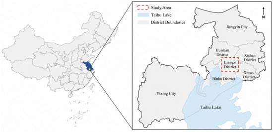
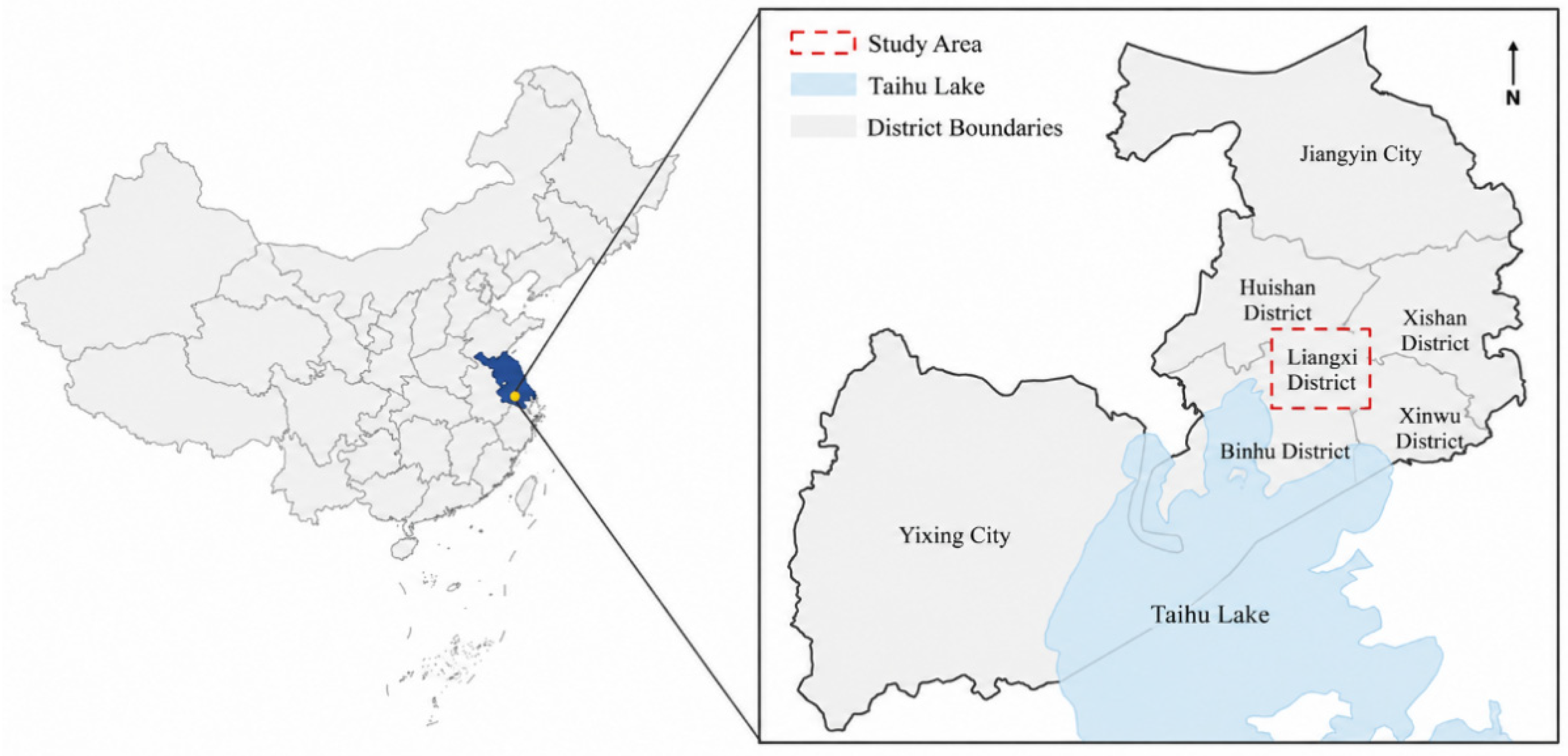
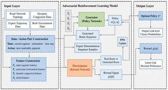
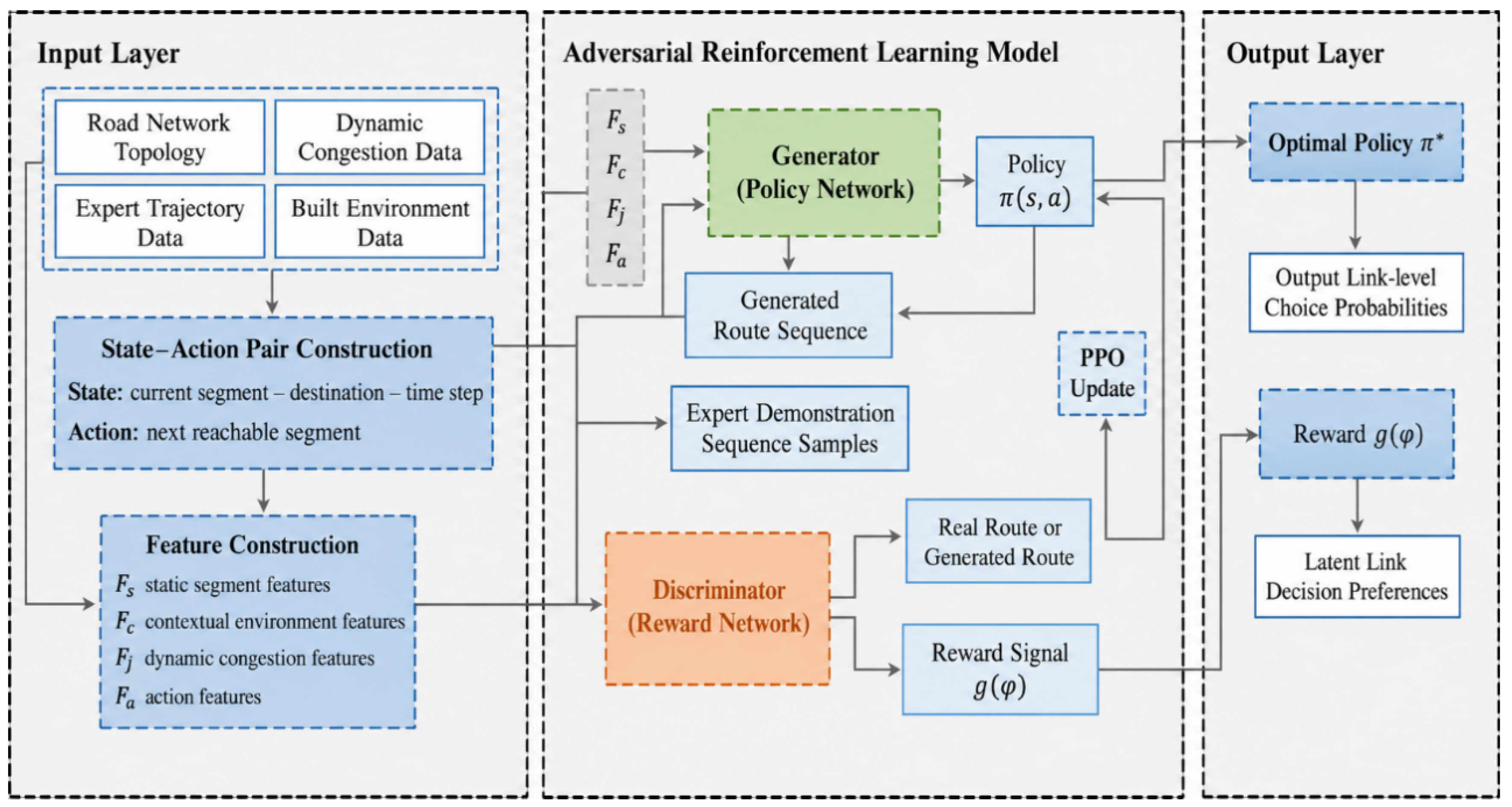
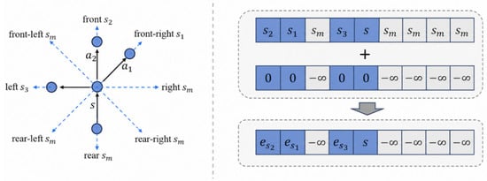
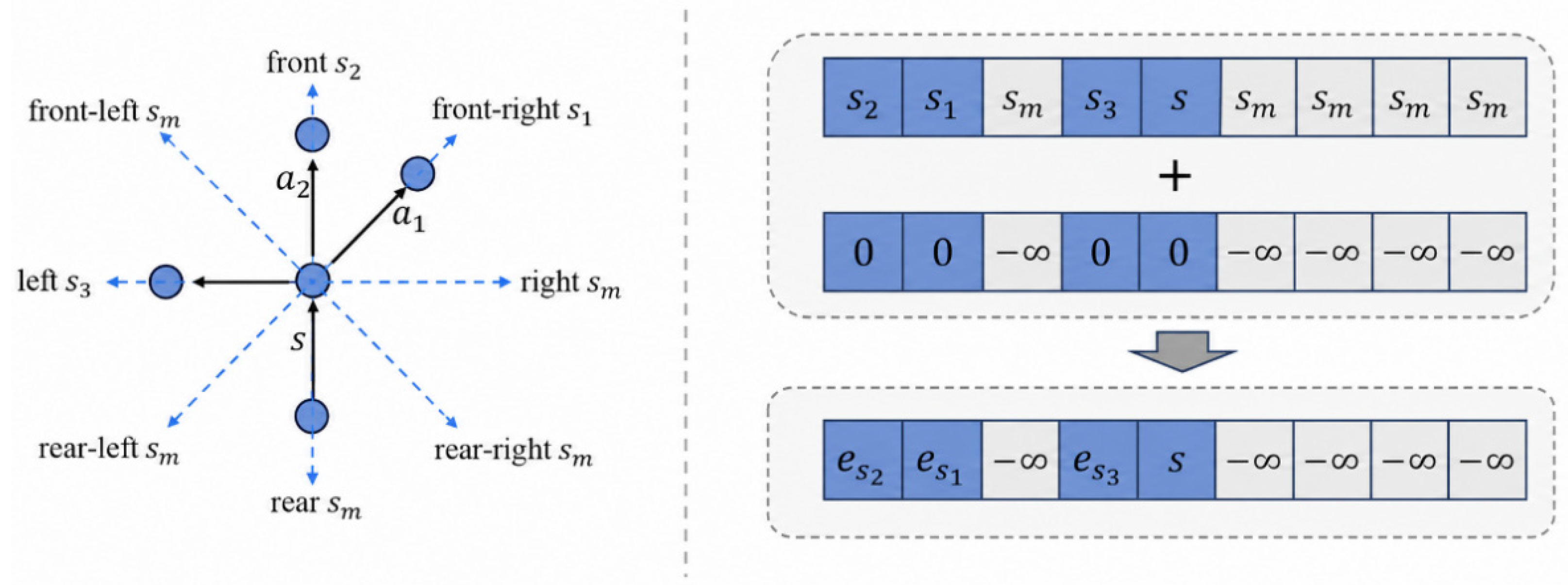
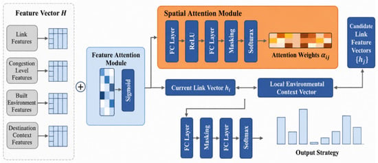
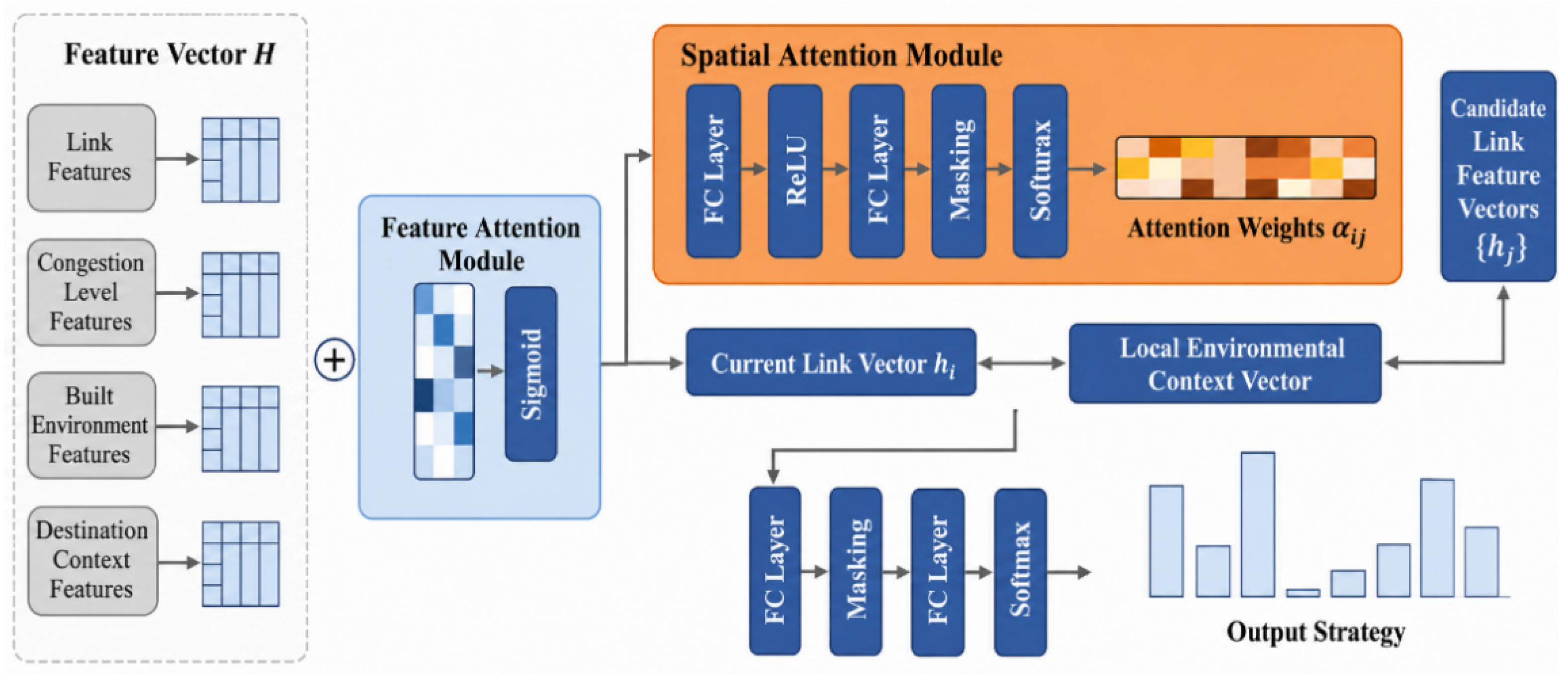
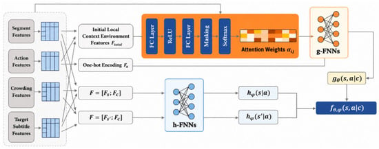
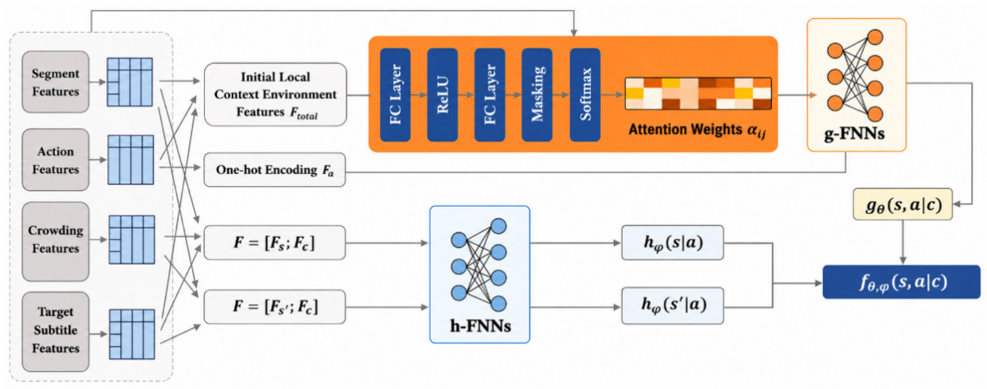
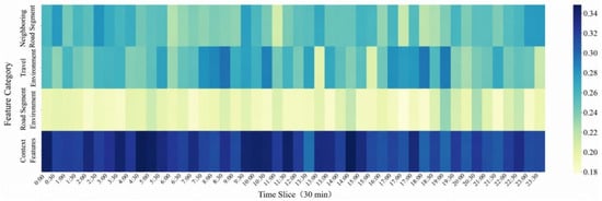
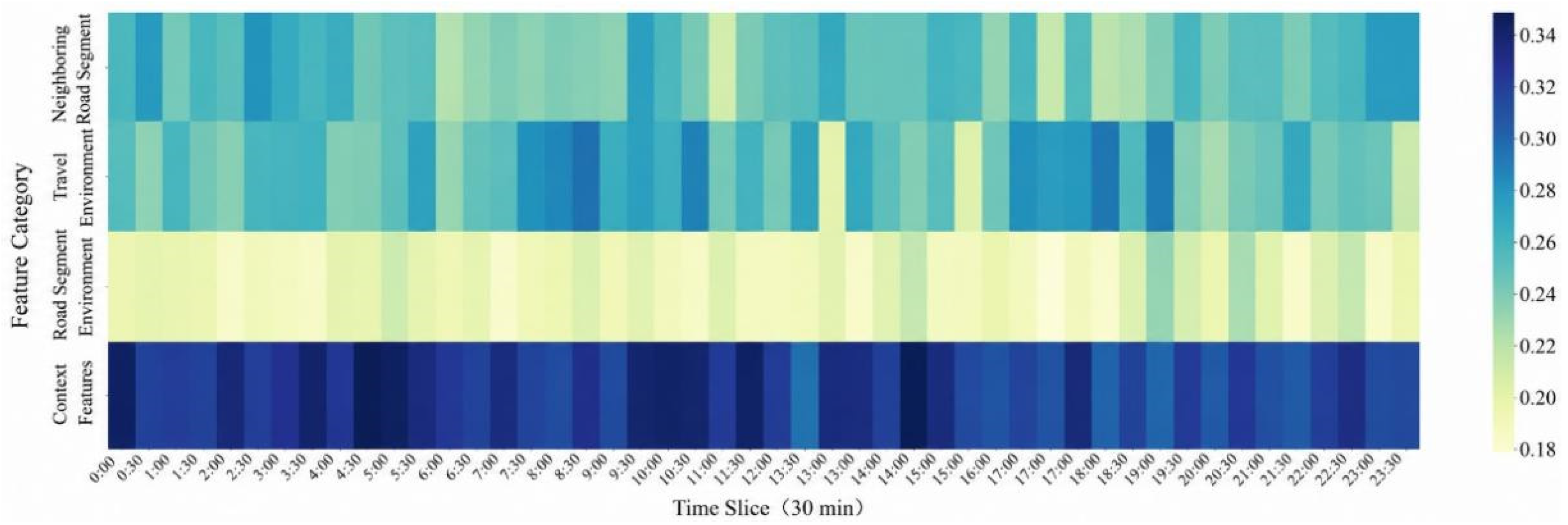
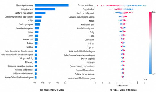
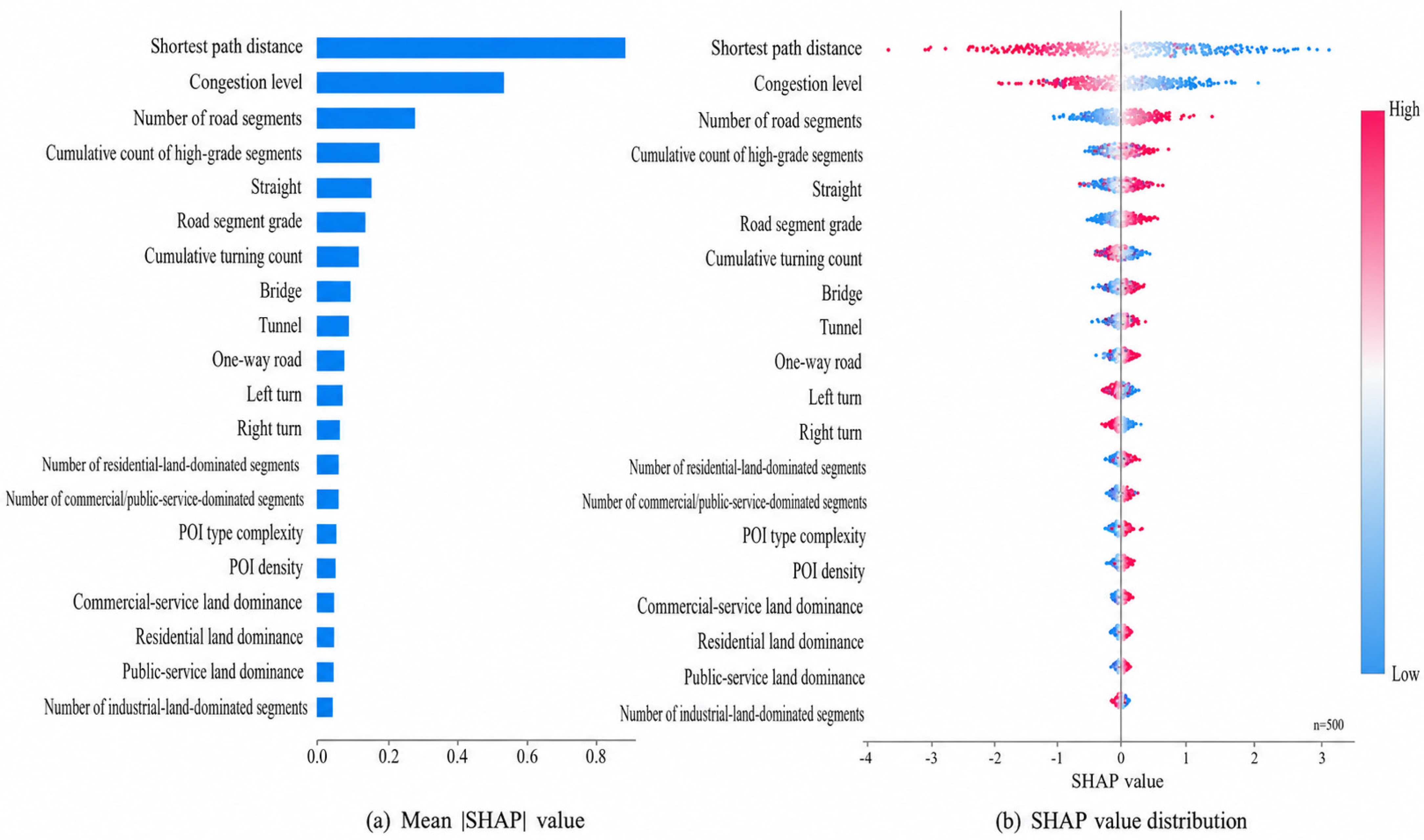
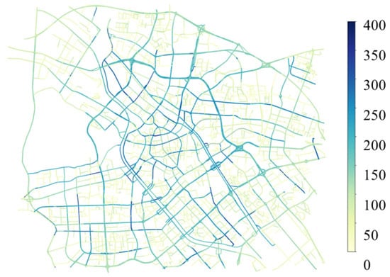
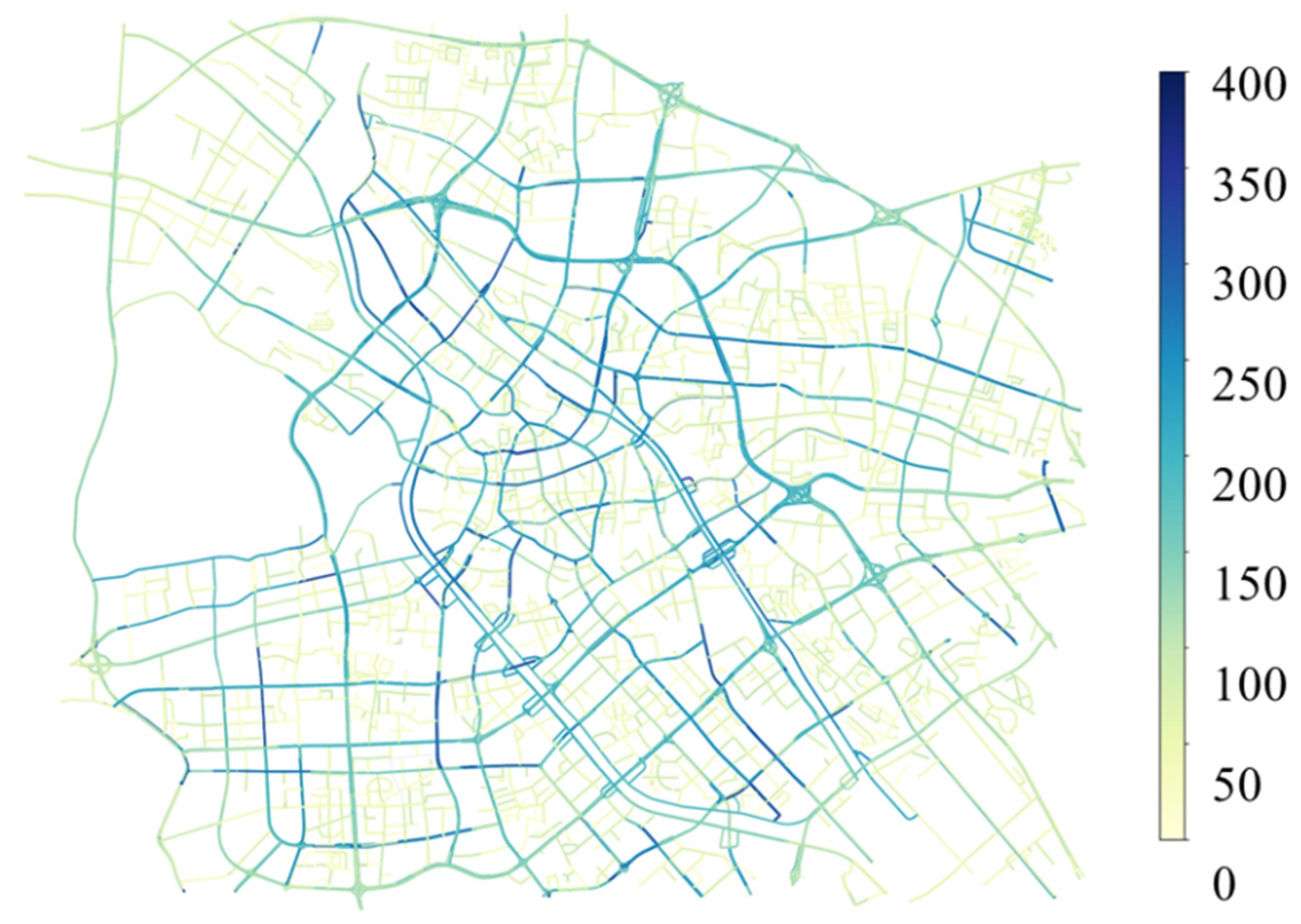
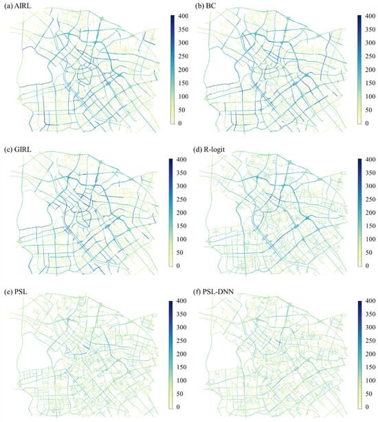
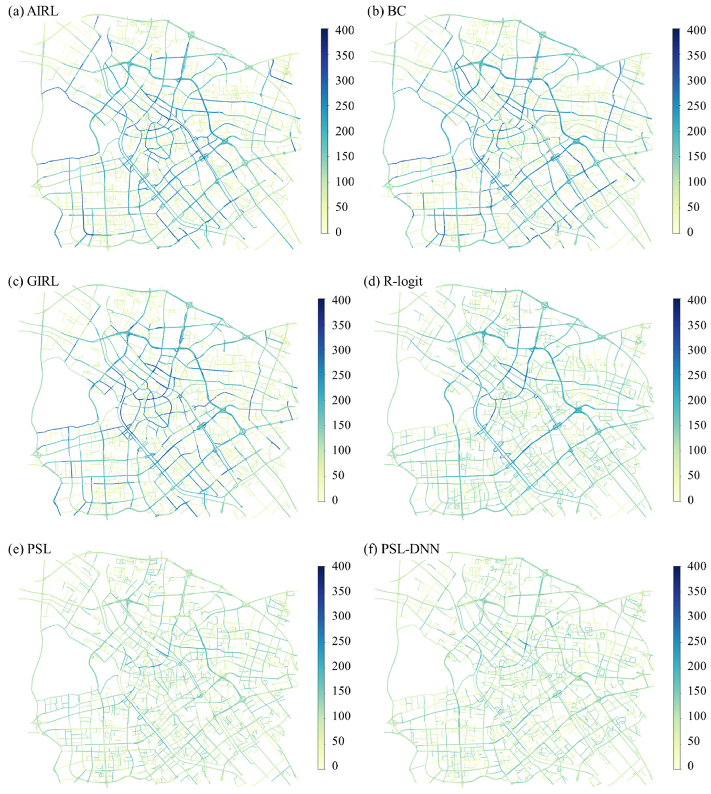

Disclaimer/Publisher’s Note: The statements, opinions and data contained in all publications are solely those of the individual author(s) and contributor(s) and not of MDPI and/or the editor(s). MDPI and/or the editor(s) disclaim responsibility for any injury to people or property resulting from any ideas, methods, instructions or products referred to in the content. |
© 2026 by the authors. Licensee MDPI, Basel, Switzerland. This article is an open access article distributed under the terms and conditions of the Creative Commons Attribution (CC BY) license.