Online Power Quality Anomaly Capture Based on Adaptive Feature Functionals and Fixed-Point Conditioning

Abstract

The large-scale integration of renewable energy loads has made distribution network waveforms strongly non-stationary. In addition to conventional harmonics and voltage deviations, power quality events with highly random triggering and extremely short durations occur frequently, posing a serious threat to precision manufacturing and high-reliability power supply scenarios. Existing detection methods, however, are either sensitive to window length and threshold settings or depend on offline labeled samples, and are therefore difficult to adapt to online anomaly discovery under continuous sampling. To address these problems, this paper proposes an online detection method based on fixed feature functionals and an adaptive normal reference. In this method, the feature centers, scales, and reliability weights are estimated only from normal windows in the training partition, and the alarm threshold is calibrated on a labeled validation partition, forming a site-adaptive online detector fitted on normal data and calibrated on a validation set. During operation, each new window is first scored against the normal reference at the previous instant, and the reference is updated only when the score falls below the update gate threshold. Experiments show that the proposed method achieves an event-level precision of 91.93%, a recall of 91.11%, and an F1 of 91.52%, providing higher detection sensitivity than comparable algorithms.

1. Introduction

The non-stationarity of distribution network waveforms arises from several mutually coupled factors. Distributed generators, such as photovoltaics and wind turbines, produce power fluctuations as resource conditions vary, load switching and nonlinear loads alter the demand and the harmonic background, and the switching and control dynamics of grid-connected and AC/DC converters further introduce ripple and transients. Reference [1] jointly investigated power fluctuation and power quality in a hybrid AC/DC microgrid containing renewable generation, energy storage, heterogeneous loads, and bidirectional converters, illustrating the severity of these effects. Such anomalies may not cause long outages, but they are sufficient to shut down sensitive loads or destabilize precision manufacturing processes. Whether subsequent mitigation equipment can start correctly depends heavily on the front-end anomaly detection result, which is therefore critical for the stable operation of precision manufacturing and large-scale data centers.

Existing power quality event detection methods generally face two typical limitations: the limited on-site computational time budget and the scarcity of on-site anomaly samples.

For the limited on-site time budget, various fast algorithms have been proposed, but their detection accuracy is often insufficient. Sliding RMS, wavelet, and time–frequency transforms respond directly to amplitude or energy changes with low computational complexity, yet their results are sensitive to window length, thresholds, and background noise [2,3,4,5,6,7]. Short windows favor early triggering but easily misjudge measurement disturbances as anomalies, whereas long windows improve statistical stability but blur short-duration anomaly signatures. Another line of work learns disturbance features from historical data through residual networks or attention models [8,9,10,11,12,13]. In recent years, one-class SVM and isolation forest detectors have been deployed directly on intelligent power quality measurement nodes, processing unlabeled load flows with normal data-driven real-time prediction [14,15]. These studies indicate that unsupervised modeling in online and edge environments must report data availability, threshold calibration, and computational boundaries at the same time. Most classification models receive pre-segmented event clips and essentially solve a post hoc recognition problem, which can hardly replace online anomaly capture under continuous sampling.

Without sufficient on-site anomaly samples, the key to online capture is to establish a normal reference that matches the current operating conditions. The load composition, background harmonics, and measurement chain of a distribution network drift slowly. A fixed template may misjudge normal drift as an anomaly, whereas unconditional updating may absorb real anomalies into the normal reference. Therefore, this paper determines the statistical basis of feature extraction using normal waveforms in the training stage, recursively updates only the normal reference during operation, and freezes the reference once the window score crosses the update gate. Because freezing is conditioned on the score crossing the gate, slowly developing or low-amplitude anomalies may alter the reference before triggering; this behavioral boundary is examined in the experiments.

To address these problems, this paper adopts a site-adaptive online detection pipeline that combines normal data fitting with validation set calibration. In the training stage, only normal windows are used to estimate feature statistics and the initial normal reference, and anomalous training records do not participate in parameter fitting. Labels in the validation stage are used only to calibrate the alarm threshold, and no parameters are tuned in the test stage. At runtime, each new window is first scored against the normal reference at the previous instant, and the score determines whether the reference is updated; the current window is never written into the reference before being scored.

The contributions of this paper are threefold:

• A fixed feature-functional dictionary driven by normal waveforms is constructed to characterize waveform morphology from physically meaningful aspects, such as amplitude and harmonic content.
• A gated recursion mechanism for the adaptive normal reference is proposed. The recursion exhibits an explicit contraction property under fixed normal input and is treated as a bounded tracking process under time-varying input; the corresponding mathematical conditions and error bounds are given in Appendix A.
• An online scoring scheme based on causal similarity attention over normal reference deviations is developed. Window deviations are organized into causal tokens according to physical groups, using only the current and limited history without training projection parameters, and event boundaries are located offline through post-processing.

2. Related Work

2.1. Combined Amplitude and Time–Frequency Detection Methods

Early power quality event detection was mainly built around statistics with clear physical meanings. Barros and Perez combined sliding RMS with event duration and amplitude estimation for the online detection of sags, swells, and interruptions [2,3,16]. The wavelet transform locates abrupt waveform changes through detail coefficients at different scales and is sensitive to steep-edged events [4]. The S transform balances time and frequency resolution and can describe local energy variations in harmonics, oscillatory transients, and compound disturbances [5,6,7]. These methods are structurally transparent with controllable computational cost, and they remain suitable as the basic front end of monitoring devices.

The limitations of such methods mainly stem from the rigidity of the windowing mechanism and the normal baseline. While amplifying local changes, wavelet and time–frequency energies also respond to noise, switching ripple, and sampling jitter [2,4,5,6]. Thresholds are usually determined from rated values or offline samples, and changes in the background spectrum after deployment are not necessarily absorbed into the normal model. This paper integrates the above interpretable physical quantities into a set of fixed feature functionals, whose feature centers, scales, and reliability weights are determined once from the normal windows of the training partition; only the normal reference vector is updated during operation.

2.2. Data-Driven Disturbance Representation and Attention Mechanisms

Open disturbance generators and deep learning models have expanded the range of event types covered by power quality analysis. Machlev et al. established a reproducible pipeline for disturbance generation and deep classification [17]. Recent studies have used convolutional, residual, and attention structures to handle noisy and compound disturbances as well as cross-platform scenarios [8,10,12], and have deployed one-class and unsupervised anomaly detection algorithms on intelligent measurement nodes or real-time load flows [14,15]. Frame–frequency attention has been used to jointly extract local correlations in three-phase time–frequency maps [11], and lightweight deep networks have been designed for edge deployment to reduce the parameter count and inference cost [13]. These works show that data-driven representations can compensate for the limited ability of a single physical indicator to describe complex waveforms, but online deployment still requires distinguishing the three stages of model training, on-site calibration, and per-window inference.

Clip recognition and online capture, however, are different tasks. Existing classification models usually receive complete pre-segmented events, and the training and test sets share similar disturbance amplitudes, durations, and noise distributions [8,11,12,13]. Even when a model maintains high accuracy on artificially noised samples, its normal baseline is still determined by the offline training set [10]. Continuous monitoring must further handle unfinished events, slowly drifting on-site normal conditions, and the prohibition of updating during anomalies. This paper treats the captured waveform clip as a potential input to an independent recognition module; the detection stage only judges whether an anomaly has occurred and estimates the event boundaries. Reference [18] combined signal processing with infrared thermography into a complete fault diagnosis chain for grid-connected photovoltaic systems, covering detection, feature analysis, and fault identification. The proposed method constitutes the detection front end of such a chain: its output time boundaries can trigger subsequent recognition and narrow the data interval to be analyzed, while providing event clips, without judging the event category or the fault cause.

2.3. Sequence Anomaly Modeling Based on Self-Attention

Recurrent structures such as LSTM model temporal dependencies through gated states [19], whereas the Transformer establishes longer-range sequence correlations through self-attention among queries, keys, and values [20]. In general multivariate time-series anomaly detection, the Anomaly Transformer constructs an anomaly criterion from association discrepancies [21], and TranAD adopts a Transformer encoder–decoder structure with self-conditioning and adversarial training to amplify the reconstruction error of anomalous samples [22]. Compared with point-wise thresholding, these methods judge local deviations within a temporal context, thereby reducing false alarms caused by isolated noise.

Existing Transformer-based anomaly detection models usually learn normal associations from offline training data, and some further rely on bidirectional context, full-window reconstruction, or iterative decoding [21,22]. This paper borrows the idea of causal attention: the deviations of the most recent eight windows from the adaptive normal reference form tokens, and a fixed cosine similarity attention aggregates current and historical evidence.

2.4. Functional Features and the Adaptive Normal Reference

Functional data analysis treats continuous curves as functional objects, describing the overall shape and local variation in a waveform through basis functions, derivatives, smoothing terms, and covariance operators [23]. This framework allows amplitude, derivatives, harmonic projections, and local time–frequency energy to enter a unified functional space. Robust signal estimation further requires that a small amount of contamination should not cause unbounded changes in the estimate, and the influence of extreme observations should be limited through bounded influence functions or residual truncation [24,25]. For online power quality monitoring, this means that the feature extraction function should adapt to normal operating conditions while not being rapidly dragged away by a newly occurring anomaly.

The Banach contraction principle gives sufficient conditions for a fixed mapping to have a unique fixed point in a complete metric space [26]. This paper applies the result only to the reference update map when the update gate is open and the candidate normal vector is fixed; with the gate closed, the map degenerates to the identity. The state in the implementation is therefore called the adaptive normal reference. The conditions and derivations for completeness, self-mapping, the contraction factor, the time-varying tracking bound, and the bounded contamination bias are given in Appendix A.1 and Appendix A.2.

Robust centers, scale normalization, residual scoring, causal attention, and online reference updating all have independent research foundations [14,15,21,22,24]. The contribution of this paper lies in coupling these components in a specific way for continuous power quality capture: the normal windows of the training partition determine the standardization and reliability weights of the 15-dimensional features; the online stage recurses the normal reference in a score-first-update-second order; and the current and historical reference deviations are aggregated into an anomaly score by causal similarity attention without trainable projections. Compared with online one-class detectors, this paper adds physical feature grouping and gated reference tracking; compared with Transformer-based detectors, it trains no query–key–value projections and uses neither future windows nor a reconstruction decoder; compared with fixed-baseline residual methods, it allows the normal reference to drift slowly in low-score windows. The novelty of this paper therefore lies in this reproducible combined pipeline and its controlled experimental performance, rather than in any of the above existing components themselves.

3. Methods

Let the sampled waveform be $x_n=x(n\Delta t)$, with sampling rate $f_s$. At time $k$, the algorithm can only access the information set generated by the current and historical windows, ${\mathcal{F}}_k$. The output is not a disturbance category but a set of abnormal events

$$\mathcal{E}=\{(t_s,t_e,d,c)\}, d=t_e-t_s,$$

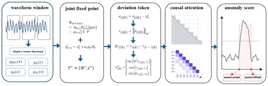
where $t_s$, $t_e$, $d$, and $c$ denote the onset, offset, duration, and capture confidence, respectively. Figure 1 shows the overall framework of the method.

Figure 1. Framework of the proposed method.

3.1. Functional Feature Construction for Power Quality Waveforms

This section defines the feature extraction mapping, whose input is a waveform window of length $L_w$ samples, denoted $x_k$, and whose output is a 15-dimensional basic feature vector. To clarify the physical origin of the features, a signal model of the normal and measured waveforms is first established. The normal grid signal is not an ideal sinusoid. For the k-th local segment, the normal waveform is written as $L_w{x}_k{z}_{k}k$

$$x_0(t;{\vartheta }_k)=A_1(t)\mathrm{s}\mathrm{i}\mathrm{n}({\omega }_{0}t+{\phi }_1(t))+\sum _{h\in {\mathcal{H}}_0}{A}_h(t)\mathrm{s}\mathrm{i}\mathrm{n}(h{\omega }_{0}t+{\phi }_h(t))+r_0(t)$$

(1)

where ${\vartheta }_k$ denotes the fundamental amplitude phase, background harmonics, and load parameters, and $r_0(t)$ denotes normal ripple and small random perturbations. The measured waveform is expressed as

$$x_m(t)=(1+{ϵ}_A)\hspace{0.17em}[x_0(t-{ϵ}_{\phi }/{\omega }_0;{\vartheta }_k)+a(t-{ϵ}_{\phi }/{\omega }_0)]+{ϵ}_b+{\eta }_m(t)$$

(2)

where $a(t)$ denotes the anomaly component, and ${ϵ}_A$,${ϵ}_{\phi }$,${ϵ}_b$ and ${\eta }_m(t)$ denote the amplitude error, phase error, zero offset, and sampling noise, respectively. A window of length $T_w=L_w/f_s$ is regarded as a function defined on $[0,T_w]$. Since $W^{1,2}$ already contains the square integrability condition, this paper directly takes the waveform space

$$\mathcal{X}=H^1([0,T_w])=W^{1,2}\left(\right[0,T_w\left]\right)$$

(3)

and the metric of waveform discrepancy is defined as follows:

$$d_{\mathcal{X}}(x_i,x_j)=\parallel x_i-x_j{\parallel }_{\mathcal{X}}$$

(4)

$$\parallel x{\parallel }_{\mathcal{X}}^2=\parallel x{\parallel }_{L^2}^2+{\lambda }_D\parallel Dx{\parallel }_{L^2}^2+{\lambda }_H\sum _{h\in \mathcal{H}}|⟨x,{\psi }_h⟩{|}^2$$

(5)

This norm specifies which waveform changes in the input space should be considered distant. It does not enter the online computation directly; its role is to delimit which feature functionals remain well-behaved under bounded inputs, and the actual feature extraction adopts the discrete implementation described below. On $\mathcal{X}$, a bounded region around the normal reference is defined as

$${\mathcal{B}}_0=\{x\in \mathcal{X}:\parallel x-x_{\mathrm{r}\mathrm{e}\mathrm{f}}{\parallel }_{\mathcal{X}}\le R_x\}$$

(6)

According to the well-posedness requirement imposed by the above norm, the feature vector finally adopted in this paper is fixed at 15 dimensions, namely RMS, peak value, crest factor, mean absolute value, RMS and maximum of the first-order difference, RMS and maximum of the second-order difference, residual energy ratio of the fundamental fitting, amplitude ratios of the 3rd and 5th harmonics, normalized spectral entropy, kurtosis, and the mean and maximum of TKEO.

Let $\Delta x_i=x_{i+1}-x_i$, ${\Delta }^2{x}_i=\Delta x_{i+1}-\Delta x_i$; let $\widehat{x}$ be the least-squares fit of the constant and nominal fundamental sine and cosine terms, $r=x-\widehat{x}$; let $A_h$ be the projection amplitude of the $h$-th harmonic and $p_m$ be the normalized positive frequency power of the windowed FFT, ${\psi }_i=x_i^2-x_{i-1}{x}_{i+1}$. The final vector is computed in order as follows:

$$\begin{gathered} [\mathrm{r}\mathrm{m}\mathrm{s}(x),\mathrm{m}\mathrm{a}\mathrm{x}|x|,{\displaystyle \frac{\mathrm{m}\mathrm{a}\mathrm{x}|x|}{\mathrm{r}\mathrm{m}\mathrm{s}(x)}},\mathrm{m}\mathrm{e}\mathrm{a}\mathrm{n}|x|,\mathrm{r}\mathrm{m}\mathrm{s}(\Delta x),\mathrm{m}\mathrm{a}\mathrm{x}|\Delta x|,\mathrm{r}\mathrm{m}\mathrm{s}({\Delta }^{2}x),\mathrm{m}\mathrm{a}\mathrm{x}|{\Delta }^{2}x|,{\displaystyle \frac{\sum r^2}{\sum x^2+\epsilon }},{\displaystyle \frac{A_3}{A_1+\epsilon }},{\displaystyle \frac{A_5}{A_1+\epsilon }}, \\ -{\displaystyle \frac{\sum p_m\mathrm{l}\mathrm{o}\mathrm{g}(p_m+\epsilon )}{\mathrm{l}\mathrm{o}\mathrm{g}M}},\mathrm{k}\mathrm{u}\mathrm{r}\mathrm{t}\mathrm{o}\mathrm{s}\mathrm{i}\mathrm{s}(x),\mathrm{m}\mathrm{e}\mathrm{a}\mathrm{n}|\psi |,\mathrm{m}\mathrm{a}\mathrm{x}|\psi |]. \end{gathered}$$

(7)

$\epsilon$ is used only to prevent division by zero. Denominator protection and finite truncation keep these discrete features bounded within the bounded input domain considered; this conclusion is not extrapolated to the zero-crossing count that is not adopted.

The normal windows of the training partition provide the per-feature median $\mu$ and the MAD robust scale $D$. The standardization is written as $z_j=\mathrm{c}\mathrm{l}\mathrm{i}\mathrm{p}({\displaystyle \frac{g_j-{\mu }_j}{D_j}},-\kappa ,\kappa )$, where $D_j$ is given a positive lower bound. The reliability weights are constructed in inverse proportion to the robust dispersion in the normal windows and then normalized to unit mean; their general form is $w_j\propto {\displaystyle \frac{b_j}{\eta +r_j}}$. The truncation bound, stabilizing term, and base weights are fixed in the validation stage and are not modified during testing.

3.2. Gated Recursion of the Adaptive Normal Reference

The initial normal reference $p_0$ is the dimension-wise median of the standardized features of the normal windows in the training partition. For the k-th window, the algorithm first uses the reference at the previous instant $p_{k-1}$ to compute the deviation $e_k=z_k-p_{k-1}$ and the current anomaly score $s_k$; the current window is never written into the reference before being scored.

Reference updating and alarm determination use two different thresholds. The algorithm first scores the current window with the reference at the previous instant; if the score is below the update gate, the reference is updated according to $p_k=(1-\alpha )p_{k-1}+\alpha c_k$, where $c_k$ is the boundedly truncated current standardized feature; otherwise $p_k=p_{k-1}$ is kept. The update rate, truncation bound, and both thresholds are determined in the validation stage and fixed in the test stage, and can be recalibrated with normal commissioning data and the allowable false alarm level during deployment.

If the update gate is open and the candidate normal vector c remains unchanged, the reference map satisfies ${∥T(p_1)-T(p_2)∥}_{\mathrm{\infty }}=(1-\alpha ){∥p_1-p_2∥}_{\mathrm{\infty }}$; when $0<\alpha <1$, it forms a contraction with respect to the reference state. If the candidate varies across windows, this equality gives only conditional single-step stability; if the update gate is closed, the map is the identity. Therefore, $p_k$ should be interpreted as gated exponential tracking of the normal state, rather than a joint fixed point guaranteed by the Banach theorem to converge under all time-varying inputs. The strict conditions and error bounds are given in Appendix A.

The gate freezes only after $s_k$ exceeds ${\tau }_u$, so weak or slowly developing disturbances may alter $p_k$ before triggering.

3.3. Causal Attention Scoring Based on Normal Reference Deviation

For each window, the algorithm compresses the reference deviation into tokens of four physical groups: distance, amplitude, transient, and spectrum. Denote the deviation vector by $e_k=z_k-p_{k-1}$ and the feature index sets of the four groups by $G_1,\dots G_4$; the group tokens are defined as

$$v_{k,g}=\sum _{j\in G_g}{w}_j\left|e_{k,j}\right|,g=1,2,3,4$$

(8)

where g = 1, 2, 3, 4 corresponds to the distance, amplitude, transient, and spectrum groups in order. The instantaneous score is a weighted sum of the four non-negative group deviations,

$${\tilde{s}}_k={\displaystyle \sum _{g=1}^4}{\beta }_g{v}_{k,g},{\beta }_g\ge 0,{\displaystyle \sum _{g=1}^4}{\beta }_g=1$$

(9)

The group weights are fixed in the validation stage; after normalization, they keep the magnitudes of different feature groups comparable and are not re-estimated on the test records.

For the current window and a finite number of historical windows, the algorithm constructs logits from token cosine similarity and a bias that decays with the time interval, and obtains the causal context through softmax. The specific form is

$${\mathcal{l}}_{k,i}={\displaystyle \frac{\mathrm{c}\mathrm{o}\mathrm{s}(v_k,v_i)}{\tau }}+b_{k-i},i=k-q+1,\dots k$$

(10)

$$a_{k,i}={\displaystyle \frac{\mathrm{e}\mathrm{x}\mathrm{p}({\mathcal{l}}_{k,i})}{{\displaystyle {\sum }_{j=k-q+1}^k}\mathrm{e}\mathrm{x}\mathrm{p}({\mathcal{l}}_{k,j})}},u_k={\displaystyle \sum _{i=k-q+1}^k}{a}_{k,i}{\tilde{s}}_i$$

(11)

The history width is determined in the validation stage. This computation accesses only current and historical tokens, uses no future windows, and has no trainable query, key, value projections, or feed-forward network; it is therefore referred to as causal similarity attention in this paper.

A lightweight recursive state is used to suppress isolated jitter. The final score consists of the instantaneous deviation, the causal context, the recursive state, and the score increment. The recursive state and the final score are written as

$$m_k=\gamma m_{k-1}+(1-\gamma ){\tilde{s}}_k,m_0=0$$

(12)

$$s_k={\lambda }_1{\tilde{s}}_k+{\lambda }_2{u}_k+{\lambda }_3{m}_k+{\lambda }_4({\tilde{s}}_k-{\tilde{s}}_{k-1})$$

(13)

The window score is available only after the 20 ms analysis window ends; causal therefore only means that the scoring does not read future windows. In the experiments, the onset and offset boundaries are obtained by mapping all window scores to sampling points through nearest-neighbor assignment, followed by short-gap filling and short-pulse removal; this step serves offline localization evaluation, may write back to the vicinity of the window center, and cannot be regarded as the real-time alarm time. The online initial alarm should be based on the window-end instant and the consecutive positive criterion, and this end-to-end timestamp has not been recorded in this paper.

3.4. Online Operation and Parameter Update Procedure

The proposed method consists of three stages: normal data fitting, validation set calibration, and per-window operation. The training partition uses only normal windows to estimate $\mu$,$D$,$w$ and $p_0$; anomalous training records do not participate in the proposed method. Labels in the validation partition are used to select the alarm thresholds of the seven methods separately, and the test partition is used only for one-shot evaluation after the thresholds are fixed. This pipeline is a site-adaptive detection scheme fitted on normal data and calibrated on a labeled validation set.

At runtime, each new window sequentially undergoes fixed feature extraction, deviation computation against the reference at the previous instant, causal attention over a finite history of tokens, anomaly scoring, current window determination, and gated reference updating. When the number of consecutive positives reaches the minimum run length, a candidate event is formed; record-level boundary consolidation is used only for the experimental localization metrics. For a fixed feature dimension $M$, analysis window length $L_w$, and finite lookback width $q$, the per-window computation is dominated by feature extraction and historical token similarity computation (Algorithm 1).

Algorithm 1. Online capture with fixed feature functionals, an adaptive normal reference, and causal attention
Input: training/validation partitions, continuously sampled waveform, window, and lookback lengths, update gate threshold, and alarm threshold
Output: window alarms and event intervals (the interval boundaries in the experiments are record-level post-processing results)
1	Estimate $\mu ,$$D,$$w$ and the initial reference using only the normal windows of the training partition $p_0$
2	Select the alarm threshold of each method separately on the validation partition $\tau$; no tuning on the test partition
3	Determine the window, lookback, update, and decision settings in the validation stage, and keep them fixed in the test stage
4	Initialize the causal state $m_0=0,$ the run-length state, and an empty event set
5	For each newly arriving window k do the following:
6	Extract the 15-dimensional features and standardize and truncate them with the training normal statistics
7	Using the reference at the previous instant $p_{k-1}$, compute the deviation and the four-dimensional token $v_k$
8	Compute the causal similarity attention context using only the current and q historical tokens
9	Compute the instantaneous score, gate value, lightweight state, and final score $s_k$
10	With $s_k>\tau ,$ form the positive decision of the current window
11	if $s_k<{\tau }_u$ then
12	After scoring, according to $p_k=(1-\alpha )p_{k-1}+\alpha c_k,$ update the bounded reference candidate
13	else set $p_k=p_{k-1},$ freezing the reference
14	Maintain candidate events according to the minimum run-length and gap-filling rules
15	When a candidate event satisfies the consecutive positive condition, issue an initial alarm at the end of the current window
16	After the record ends, reconstruct and consolidate event boundaries only for experimental evaluation
17	Save the window score, decision, and current reference
18	end for

4. Results

4.1. Data Sources

The experimental data consist of field-collected waveform samples covering ten categories: normal, voltage sag, voltage swell, short interruption, harmonics, flicker, notch, spike, impulsive transient, and oscillatory transient, with 100 samples per category. Each sample contains 4000 sampling points at an interval of 100 μs, corresponding to a 10 kHz sampling rate and a duration of 0.4 s, and the category label is given by the file name. All nine anomaly categories come from acquisition records. In actual grid-connected testing, it is impossible to preset whether an abnormal event will occur in the grid, and no corresponding standard test equipment is available. Therefore, standard test instruments capable of simulating actual grid operation are required. To emulate actual grid conditions, amplitude variations, background harmonics, slow drift, and measurement noise are superimposed on the collected power quality anomaly data.

The anomaly onset and offset boundaries are not generated by the anomaly score of the proposed method. Before model inference, the evaluation program compares the waveform of each anomalous sample point by point with the same normal template, uses $\mathrm{m}\mathrm{a}\mathrm{x}({10}^{-10},{10}^{-7}·\mathrm{m}\mathrm{a}\mathrm{x}|x_{\mathrm{n}\mathrm{o}\mathrm{r}\mathrm{m}\mathrm{a}\mathrm{l}}|)$ as the amplitude tolerance, and removes difference segments shorter than two sampling points to form a reference mask, which is used to verify whether the experimental results are correct.

4.2. Experimental Platform

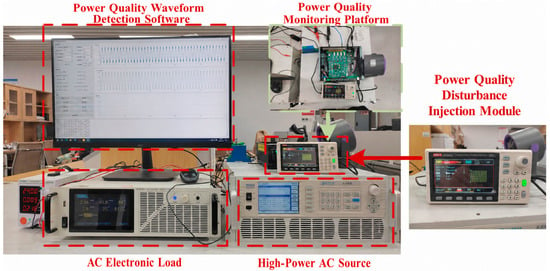
As shown in Figure 2, a standard arbitrary waveform generator, an AC power source with loads, and a PCIe acquisition chain are used to generate and acquire the test waveforms. The peak sampling rate of the acquisition card is 5 MSPS. The embedded acquisition terminal is configured with an Intel i5-6500 and 8 GB of memory. The embedded acquisition architecture needs to distinguish the front-end sampling, A/D conversion, transmission, and local processing stages [27]. This paper reports only the average time of preprocessing, feature extraction, scoring, and binarization after the waveform is loaded, which is used for comparison within the same offline environment. The formation time of a 20 ms window is determined by the analysis window length; acquisition, PCIe transmission, storage, and alarm generation are not counted, so this result is not equivalent to the end-to-end latency of a complete system. The device latency may vary with the hardware implementation, but the overall latency, throughput, memory, or power consumption cannot be inferred before measurement.

Figure 2. Experimental platform.

4.3. Experimental Configuration and Evaluation Metrics

The sparse autoencoder and the Causal LSTM predictor are both trained only with the normal windows of the training partition. The former adopts a 15-8-15 structure and uses the root-mean-square reconstruction error of the standardized features as the anomaly score [28]; the latter adopts a unidirectional LSTM with 24 hidden units, predicts the next window from the historical features up to the current window, and uses the one-step prediction error as the anomaly score [29]. Both use the same base sample partition, 20 ms window, 2 ms step, validation set threshold selection rule, and test evaluation procedure as the other methods, and the test labels do not participate in model training or threshold selection.

To evaluate the stability of the same base sample under varying measurement disturbances, two disturbed samples are generated for each validation base sample, giving 400 validation samples, and five disturbed samples are generated for each test base sample, giving 1000 test samples, i.e., 100 per category. The disturbance factors include a cyclic time shift of no more than 4 ms, an amplitude variation of ±2%, Gaussian noise of 0.05–0.35%, low-amplitude 3rd/5th background harmonics, and a slow amplitude drift of 0.3–0.8 Hz. The number of independent base samples remains 200, i.e., 20 per category. The 1000 test samples are correlated repeated measurements of these base samples and are used for disturbance robustness evaluation; they cannot be interpreted as 1000 independent test sources, nor can it be claimed that the limitation of a small independent test set has been eliminated. Confidence intervals and paired tests take the base sample as the clustering unit, with each cluster containing the five disturbed samples of that sample.

All methods are compared under the same sampling, windowing, data partitioning, and validation set threshold selection protocols. The internal truncation, reference updating, lookback, and event consolidation parameters of the proposed method are determined using only the training and validation partitions and remain fixed during testing. These settings ensure the consistency of the comparison within this study. At a new monitoring site, recalibration can be performed with normal commissioning data according to the background fluctuation and the allowable false alarm level.

To avoid mixing levels, this paper reports event-level and binary window-level metrics separately. Event-level statistics take the single reference event in each anomalous sample as the unit: a prediction interval overlapping the reference interval is counted as ${\mathrm{T}\mathrm{P}}_e$, no overlap is counted as ${\mathrm{F}\mathrm{N}}_e$, and a prediction on a normal sample or a prediction on an anomalous sample that completely deviates from the reference interval is counted as ${\mathrm{F}\mathrm{P}}_e$. The event-level precision, recall, and F1 are defined as follows:

$$P_e={\displaystyle \frac{{\mathrm{T}\mathrm{P}}_e}{{\mathrm{T}\mathrm{P}}_e+{\mathrm{F}\mathrm{P}}_e}};R_e={\displaystyle \frac{{\mathrm{T}\mathrm{P}}_e}{{\mathrm{T}\mathrm{P}}_e+{\mathrm{F}\mathrm{N}}_e}};{\mathrm{F}1}_e={\displaystyle \frac{2P_e{R}_e}{P_e+R_e}}$$

(14)

The window-level $P_w$, $R_w$ and ${\mathrm{F}1}_w$ are computed directly from the binary decisions of 20 ms windows, and the event-level results are always denoted by $P_e$, $R_e$ and ${\mathrm{F}1}_e$.

$${\mathrm{P}}_{\mathrm{w}}={\displaystyle \frac{{\mathrm{T}\mathrm{P}}_{\mathrm{w}}}{{\mathrm{T}\mathrm{P}}_{\mathrm{w}}+{\mathrm{F}\mathrm{P}}_{\mathrm{w}}}};{\mathrm{R}}_{\mathrm{w}}={\displaystyle \frac{{\mathrm{T}\mathrm{P}}_{\mathrm{w}}}{{\mathrm{T}\mathrm{P}}_{\mathrm{w}}+{\mathrm{F}\mathrm{N}}_{\mathrm{w}}}}$$

(15)

$${\mathrm{F}1}_w={\displaystyle \frac{2P_w{R}_w}{P_w+R_w}}$$

(16)

The interval localization quality is evaluated by the temporal intersection over union (tIoU), and the absolute errors of the onset and offset boundaries are also reported. For the 300 s continuous normal stream, the number of false alarm events per hour and the number of false alarm windows per 100,000 windows are counted, as defined below.

$$tIoU={\displaystyle \frac{\left|I_{\mathrm{p}\mathrm{r}\mathrm{e}\mathrm{d}}\cap I_{\mathrm{r}\mathrm{e}\mathrm{f}}\right|}{\left|I_{\mathrm{p}\mathrm{r}\mathrm{e}\mathrm{d}}\cup I_{\mathrm{r}\mathrm{e}\mathrm{f}}\right|}}$$

(17)

$${\mathrm{F}\mathrm{A}\mathrm{R}}_h={\displaystyle \frac{N_{\mathrm{F}\mathrm{A}}}{T}}\times 3600;{\mathrm{F}\mathrm{A}\mathrm{R}}_{100\mathrm{k}}={\displaystyle \frac{N_{\mathrm{F}\mathrm{P},w}}{N_w}}\times {10}^5$$

(18)

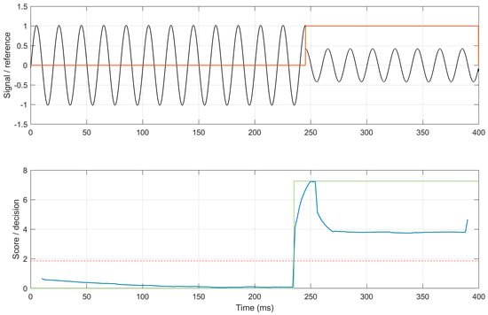
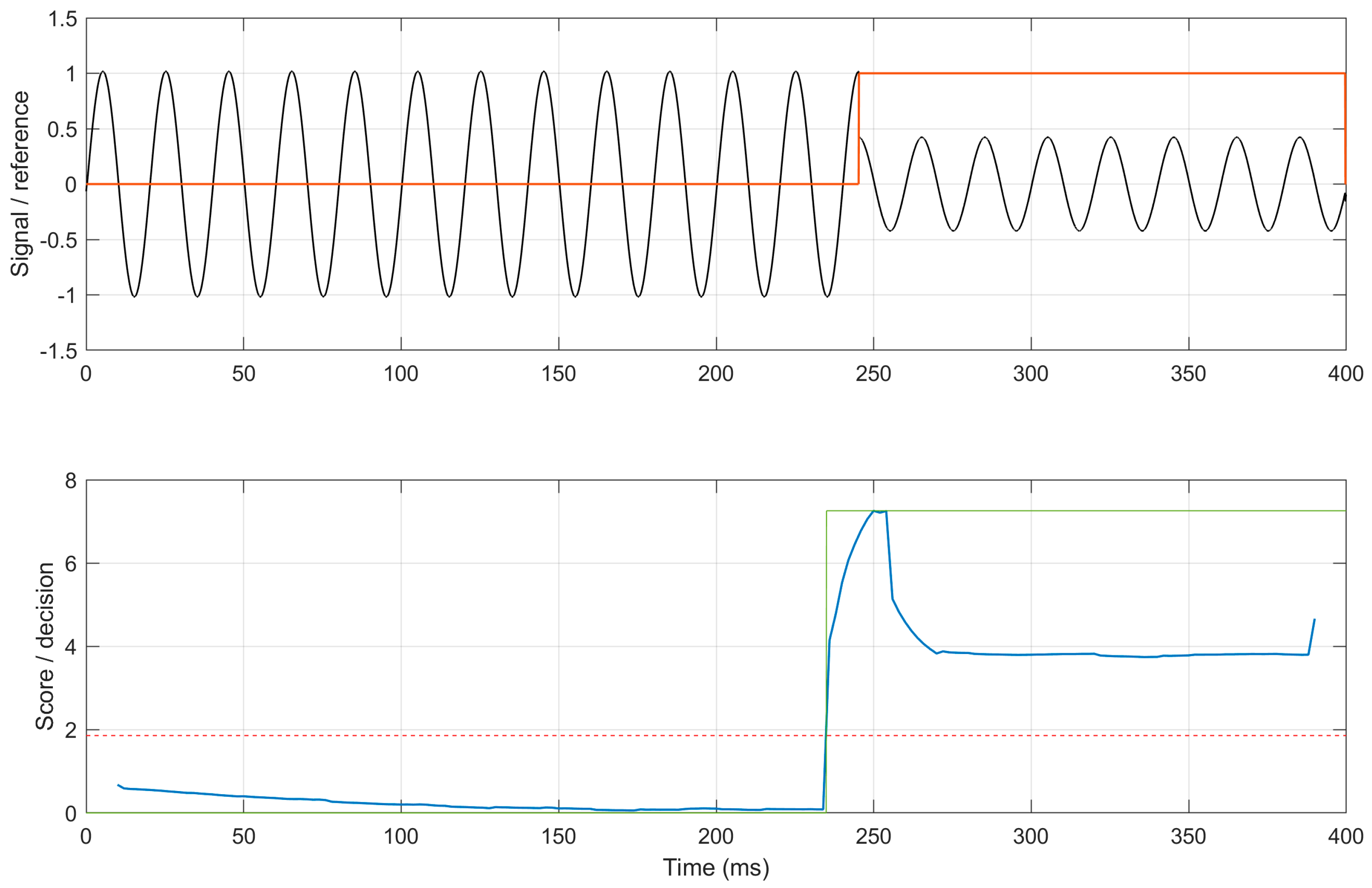
The 95% confidence interval of the event-level F1 is obtained by 1000 bootstrap replications clustered by the 200 held-out base samples, with all five disturbed samples of a base sample included whenever it is drawn. Per-sample exact McNemar tests and sign tests aggregated by base sample are reported between methods. Since the disturbed samples of the same base sample are not mutually independent, the more conservative base sample clustered conclusions are adopted in the main text (Figure 3).

Figure 3. A representative voltage sag sample and the detection result.

4.4. Ablation Under Two Threshold Calibration Protocols

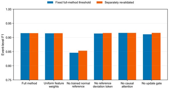
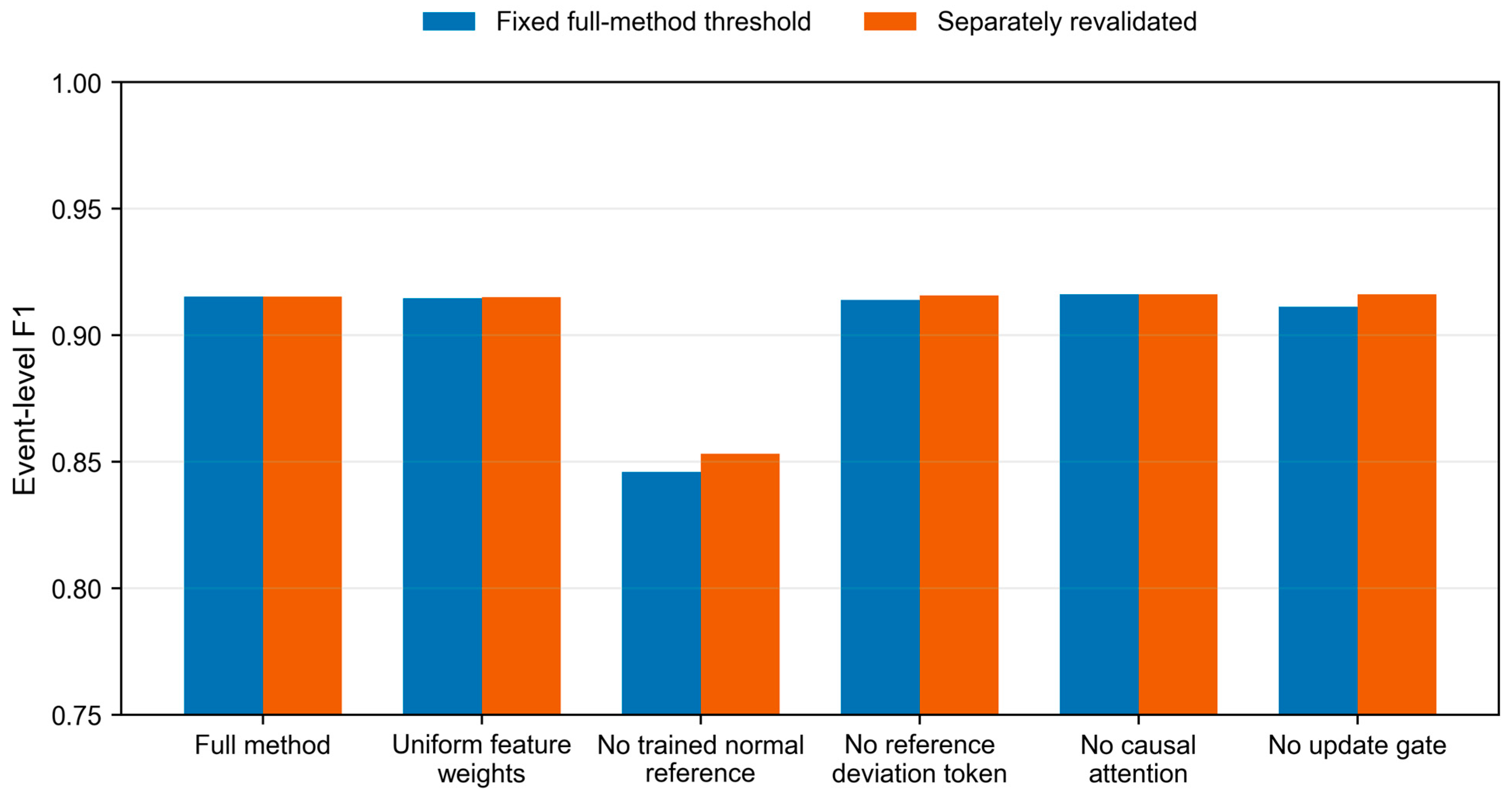
The ablation experiments adopt two calibration protocols. The first fixes the alarm threshold determined by the full method on the validation set to all variants, so as to observe the effects of structure removal and score-scale changes simultaneously; the second allows each variant to reselect the alarm threshold only on the same validation set, so as to compare the achievable performance after fair calibration. These two protocols are unrelated to the trigger-and-release dual thresholds at runtime.

Table 1 shows that the event-level F1 values of uniform feature weights and of the variant without the reference deviation token are 91.51% and 91.57%, respectively, which are close to the 91.52% value of the full method. After replacing the trained normal reference with the median of the first three windows of the current record, the revalidated F1 still drops to 85.31% and the median tIoU is only 5.00%, indicating that the trained normal reference directly contributes to detection and localization. The median tIoU without the update gate is 35.66%, which is lower than 42.14% of the full method. These ablation results therefore clearly support the positive effect of the trained normal reference on the recognition rate (Figure 4).

Table 1. Ablation results with the full-method alarm threshold fixed and with thresholds separately revalidated for each variant (%).

Variant	${\mathbf{F}1}_{\mathit{e}}$/Fixed	Median tIoU/Fixed	${\mathbf{F}1}_{\mathit{e}}$/Revalidated	Median tIoU/Revalidated	False Alarms on Normal Records/Revalidated
Full model	91.52	42.14	91.52	42.14	2.00
Uniform feature weights	91.47	42.14	91.51	45.95	0.00
No trained normal reference	84.59	5.40	85.31	5.00	2.00
No reference deviation token	91.40	43.62	91.57	41.96	1.00
No causal attention	91.62	46.58	91.62	46.58	0.00
No update gate	91.13	35.88	91.62	35.66	0.00

Figure 4. Event-level F1 with the full-method alarm threshold fixed and with thresholds separately revalidated for each variant.

4.5. Comparative Experiments

Table 2 checks all counts and arithmetic relations at the event level. The evaluation set contains 1000 correlated test samples, of which 900 are anomalous and 100 are normal. ${\mathrm{T}\mathrm{P}}_e$, ${\mathrm{F}\mathrm{P}}_e$, and ${\mathrm{F}\mathrm{N}}_e$ are first obtained by event matching on each sample, and $P_e$, $R_e$, and ${\mathrm{F}1}_e$ are then computed uniformly. The integers in the table are sample-level counts, and the statistical uncertainty is estimated by base sample clustering. These results therefore reflect the detection stability of the held-out base samples under repeated measurement disturbances.

Table 2. Event-level results on 1000 correlated disturbance samples generated from 200 held-out base samples.

Method	${\mathbf{T}\mathbf{P}}_{\mathit{e}}$	${\mathbf{F}\mathbf{P}}_{\mathit{e}}$	${\mathbf{F}\mathbf{N}}_{\mathit{e}}$	${\mathit{P}}_{\mathit{e}}$	${\mathit{R}}_{\mathit{e}}$	${\mathbf{F}1}_{\mathit{e}}$	False Alarms on Normal Records
RMS event	654	175	246	78.89	72.67	75.65	77.00
Wavelet energy	620	79	280	88.70	68.89	77.55	9.00
STFT/S transform	675	12	225	98.25	75.00	85.07	1.00
TKEO energy	696	62	204	91.82	77.33	83.96	7.00
Sparse AE	715	70	185	91.08	79.44	84.87	0.00
Causal LSTM	717	72	183	90.87	79.67	84.90	0.00
Proposed	820	72	80	91.93	91.11	91.52	2.00

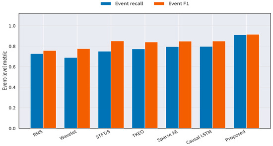
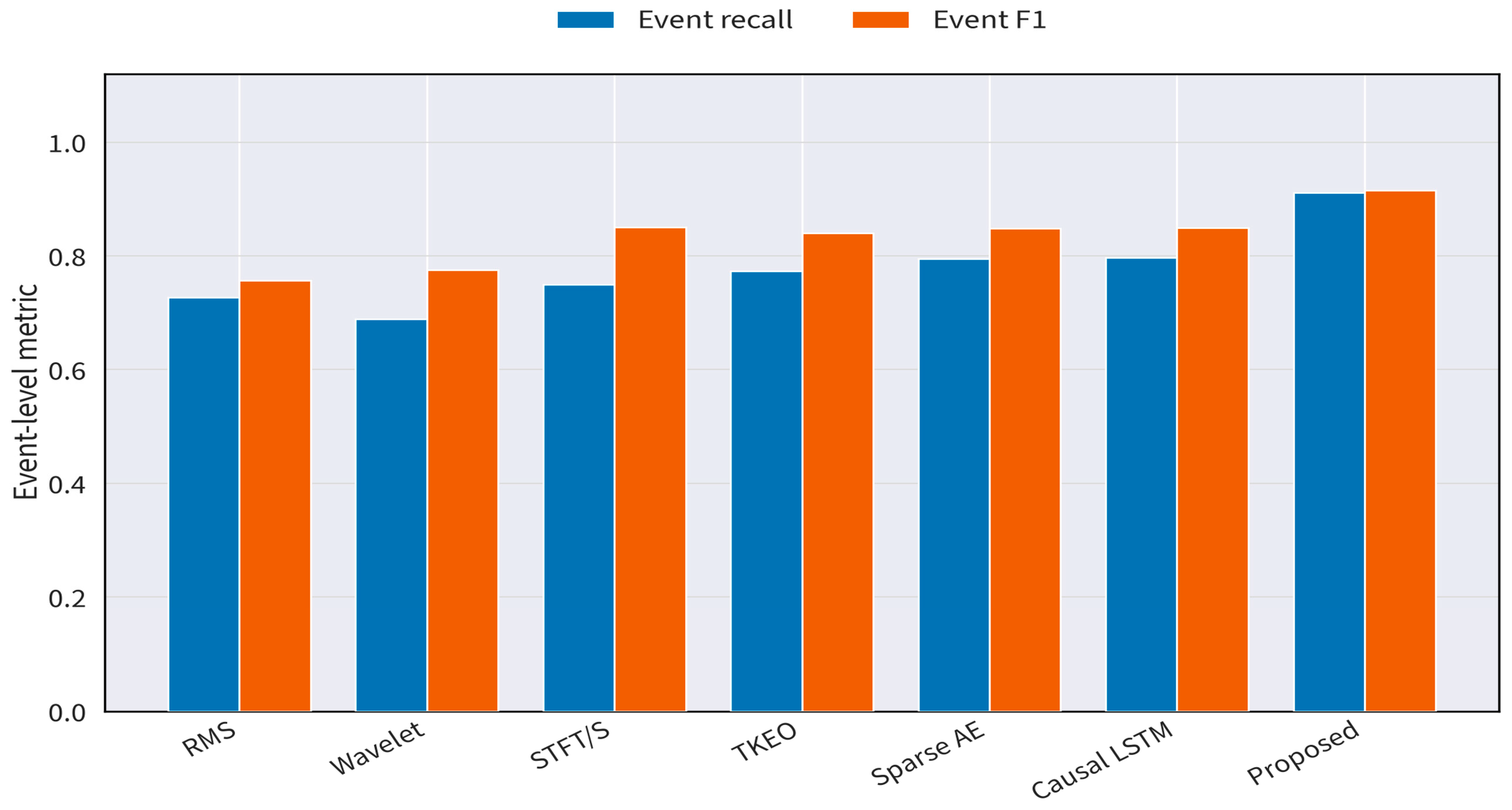
On the 1000 correlated disturbance samples, the event-level precision, recall, and F1 of the proposed method are 91.93%, 91.11%, and 91.52%, respectively. The event-level F1 values of Sparse AE and Causal LSTM are 84.87% and 84.90%, with the p-values of the paired sign tests aggregated by base sample both equal to 1.0000. The event-level F1 of STFT/S transform is 85.07%, and the proposed method achieves the highest event-level F1 among the seven methods (Figure 5). Relative to RMS event and TKEO energy, the base sample clustered decision advantages of the proposed method are both p < 0.01; relative to Wavelet energy, the advantage is not significant (p = 0.0625). Therefore, the present results only support that the proposed method is competitive under the common held-out samples and the disturbance repeated measurement protocol, and do not support the conclusion of overall superiority over traditional and learning-based baselines (Table 3).

Figure 5. Event-level recall and F1 of all methods on the correlated disturbance samples.

Table 3. Binary window-level and time interval-level results (%, with boundary errors and runtime in ms).

Method	${\mathit{P}}_{\mathit{w}}$/${\mathit{R}}_{\mathit{w}}$/${\mathbf{F}1}_{\mathit{w}}$	Mean tIoU	Median tIoU	Median Onset/Offset Absolute Error	Per-Record Time
RMS event	37.80/65.76/48.01	27.53	4.81	22.00/10.45	17.42
Wavelet energy	93.69/99.29/96.41	46.88	44.17	9.60/9.50	17.21
STFT/S transform	99.78/88.91/94.03	41.02	28.90	9.20/9.20	17.48
TKEO energy	90.54/53.53/67.28	24.00	10.33	9.80/9.70	18.50
Sparse AE	93.86/99.82/96.75	47.66	48.25	9.50/9.50	15.98
Causal LSTM	93.86/99.88/96.78	47.65	48.25	9.50/9.50	15.50
Proposed	92.47/99.96/96.07	45.91	42.14	9.55/13.10	18.80

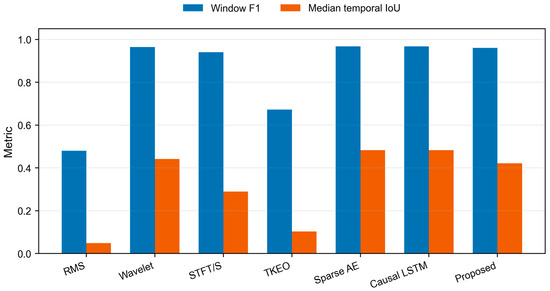
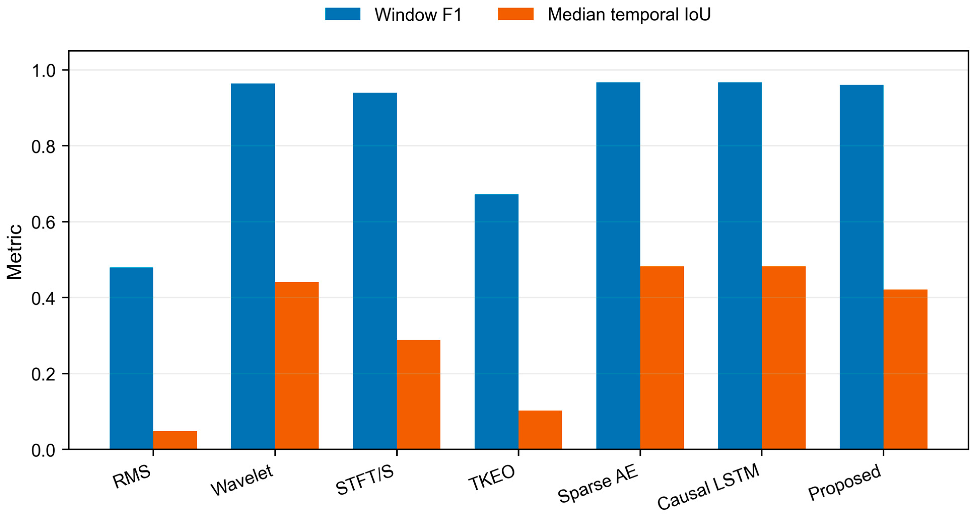
In the binary window-level evaluation, the window-level F1 values of all methods are generally close: the proposed method achieves 96.07%, differing from the 96.41%, 96.75%, and 96.78% of Wavelet energy, Sparse AE, and Causal LSTM by less than one percentage point, so its recognition accuracy is basically comparable to existing methods. The window-level recall of the proposed method reaches 99.96%, which is the highest among the seven methods (Figure 6). The mean and median tIoU of the proposed method are 45.91% and 42.14%, and the median absolute onset/offset errors are 9.55/13.10 ms; the median tIoU values of the two learning baselines are both 48.25%, which is slightly higher than that of the proposed method. However, almost no anomalous window is missed under the 20 ms analysis window, indicating that the proposed method can form consecutive positive decisions faster after an event occurs, with higher detection sensitivity and more timely capture, and its detection rate is significantly higher than that of the compared methods (Table 4).

Figure 6. Window-level F1 and median temporal IoU of all methods.

Table 4. False alarm stress test on the 300 s continuous normal stream.

Method	Windows	False Alarm Events	False Alarm Events/h	False Alarm Windows/100 k
RMS event	149,991	223	2676.00	46,416.12
Wavelet energy	149,991	0	0.00	0.00
STFT/S transform	149,991	4368	52,416.00	67,008.69
TKEO energy	149,991	0	0.00	0.00
Sparse AE	149,991	0	0.00	0.00
Causal LSTM	149,991	0	0.00	0.00
Proposed	149,991	0	0.00	0.00

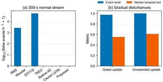
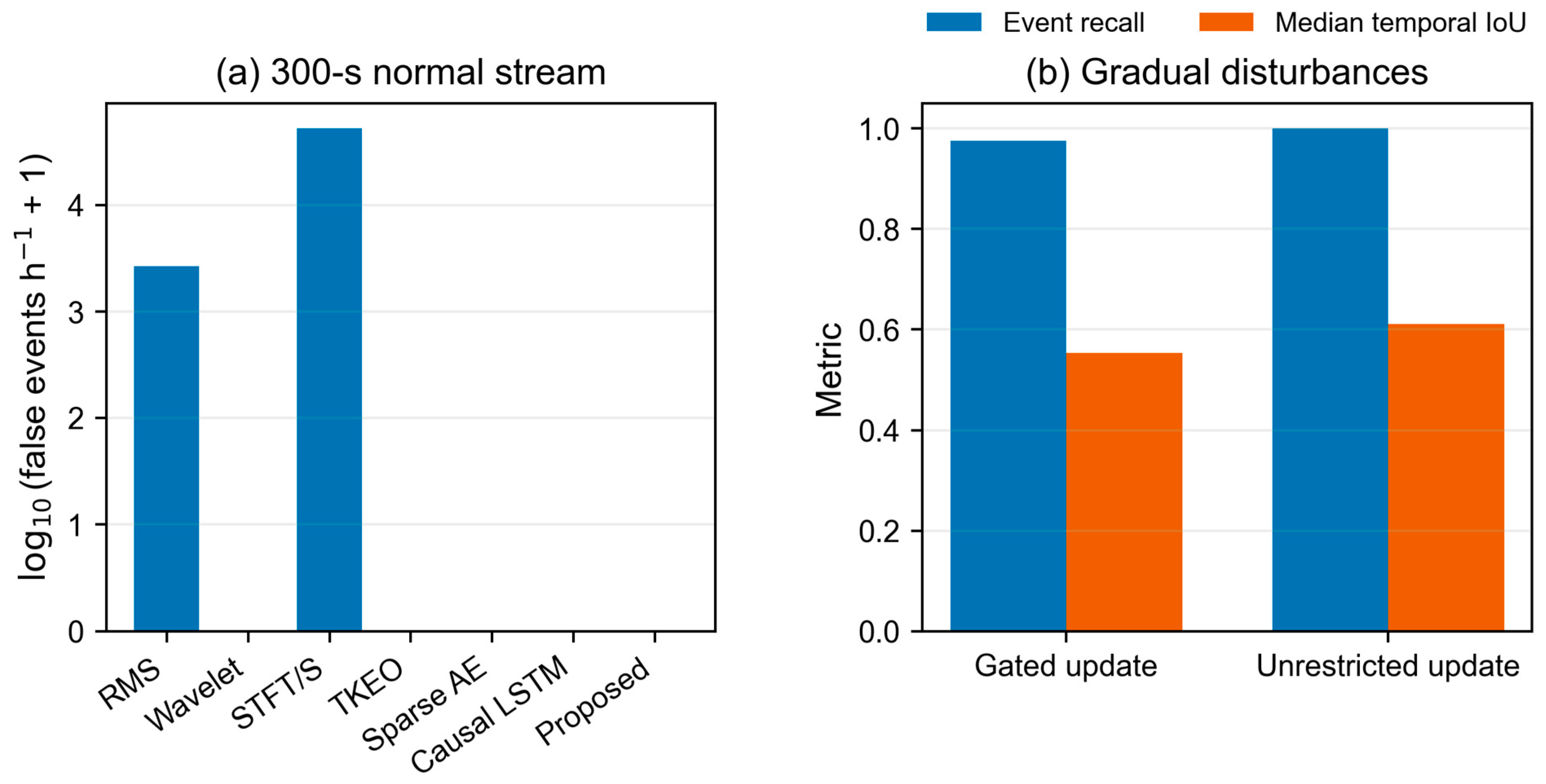
The 300 s continuous normal stream contains 149,991 overlapping windows. The proposed method produces 0 false alarm events, i.e., 0.00 events/h and 0.00 false alarm windows per 100,000 windows. This result is the same as Wavelet energy, TKEO energy, Sparse AE, and Causal LSTM, and lower than RMS event and STFT/S transform. Among them, STFT/S transform produces 4368 false alarm events and maintains a high density of positive windows.

Similarly, on 200 slowly developing sag and harmonic events, the event recall of gated updating is 97.50%, which is lower than the 100.00% of unrestricted updating, and the median tIoU values are 55.41% and 61.16%, respectively. The median onset lags computed from the record-level reconstructed intervals are 73.1 ms and 59.1 ms, respectively. The gate slightly reduces the median final-state RMS shift of the standardized normal reference from 0.684 to 0.647, but at the cost of capture and localization performance. The current update gate therefore demonstrates a certain suppression effect on reference drift.

Measurement data drift slowly changes the normal statistical characteristics of the waveform, gradually deviates a fixed reference from the real operating conditions, and consequently causes false alarms or missed alarms, which is a problem that cannot be ignored in online detection. The proposed method adaptively updates the normal reference through gated recursion, which can suppress the reference shift caused by drift to a certain extent. Therefore, although its detection performance does not significantly exceed that of other algorithms, it has stronger applicability in practical scenarios with data drift (Figure 7).

Figure 7. Verification on the continuous normal stream and gradual disturbances. (a) The number of false alarm events per hour on the 300 s normal stream, displayed as log10 (value + 1); (b) event recall and median tIoU of gated and unrestricted updating.

4.6. Algorithm Performance Analysis

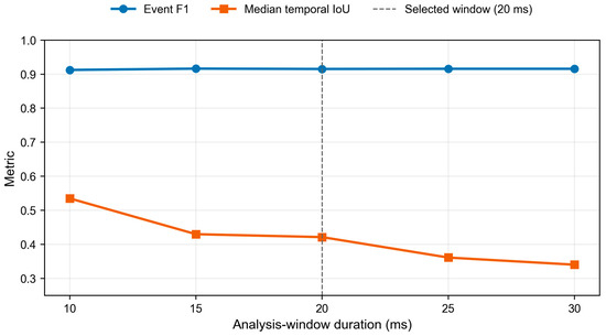
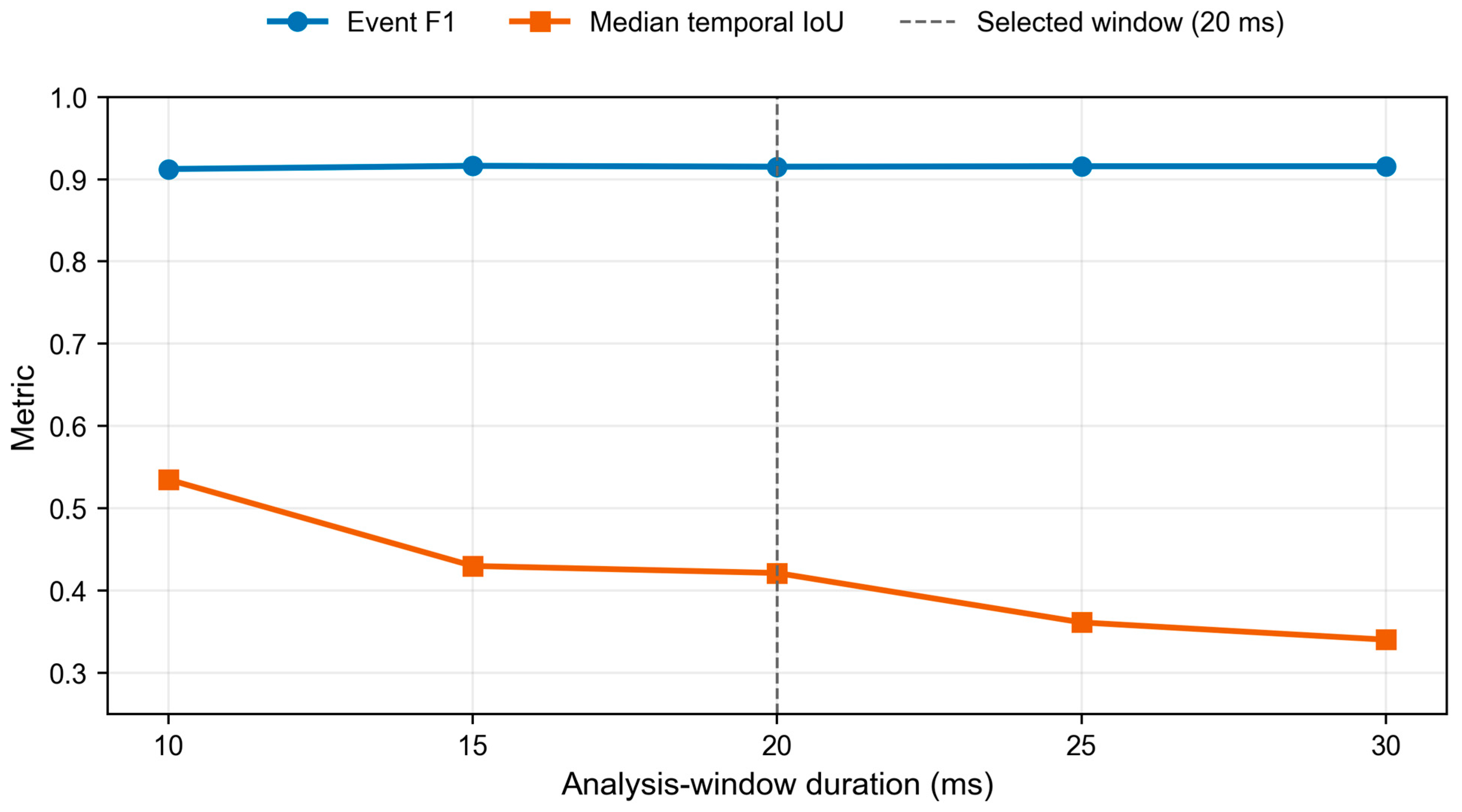
The window length is analyzed by one-factor sensitivity analysis. Except for the candidate window length, all other processing, data partitioning, and threshold selection rules remain unchanged. Each candidate setting is recalibrated only on the validation samples and then evaluated on the same test samples. Table 5 gives the window lengths and the corresponding detection results, and Figure 8 shows the performance changes in unified coordinates.

Table 5. One-factor sensitivity analysis of the window length.

Window Length, Points/ms	${\mathit{P}}_{\mathit{e}}/{\mathit{R}}_{\mathit{e}}/{\mathbf{F}1}_{\mathit{e}}$(%)	Median tIoU/%
100/10	94.84/87.89/91.23	53.50
150/15	92.13/91.11/91.62	43.00
200/20	91.93/91.11/91.52	42.14
250/25	92.03/91.11/91.57	36.14
300/30	92.03/91.11/91.57	34.04

Figure 8. Effect of the analysis window length on the event-level F1 and the median temporal IoU.

On the test platform, the per-sample algorithm time of the proposed method, measured from the waveform already loaded in memory and including feature extraction and per-window scoring, has a mean of 20.05 ms, a median of 19.21 ms, a 95th percentile of 25.90 ms, and a maximum of 36.67 ms. The persistent model array occupies 1184 B, which excludes software runtime events, acquisition buffering, and operating system overhead. Since the core work of this paper is the detection algorithm, the external hardware chain of the detection system is unrelated to the proposed method; therefore, the latency generated by the acquisition hardware was not measured synchronously on the same instrument chain.

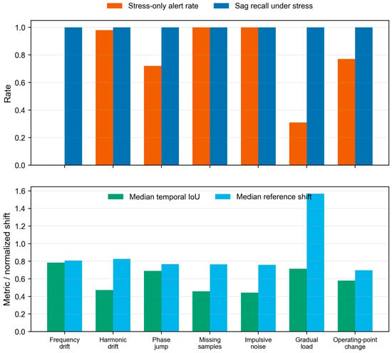
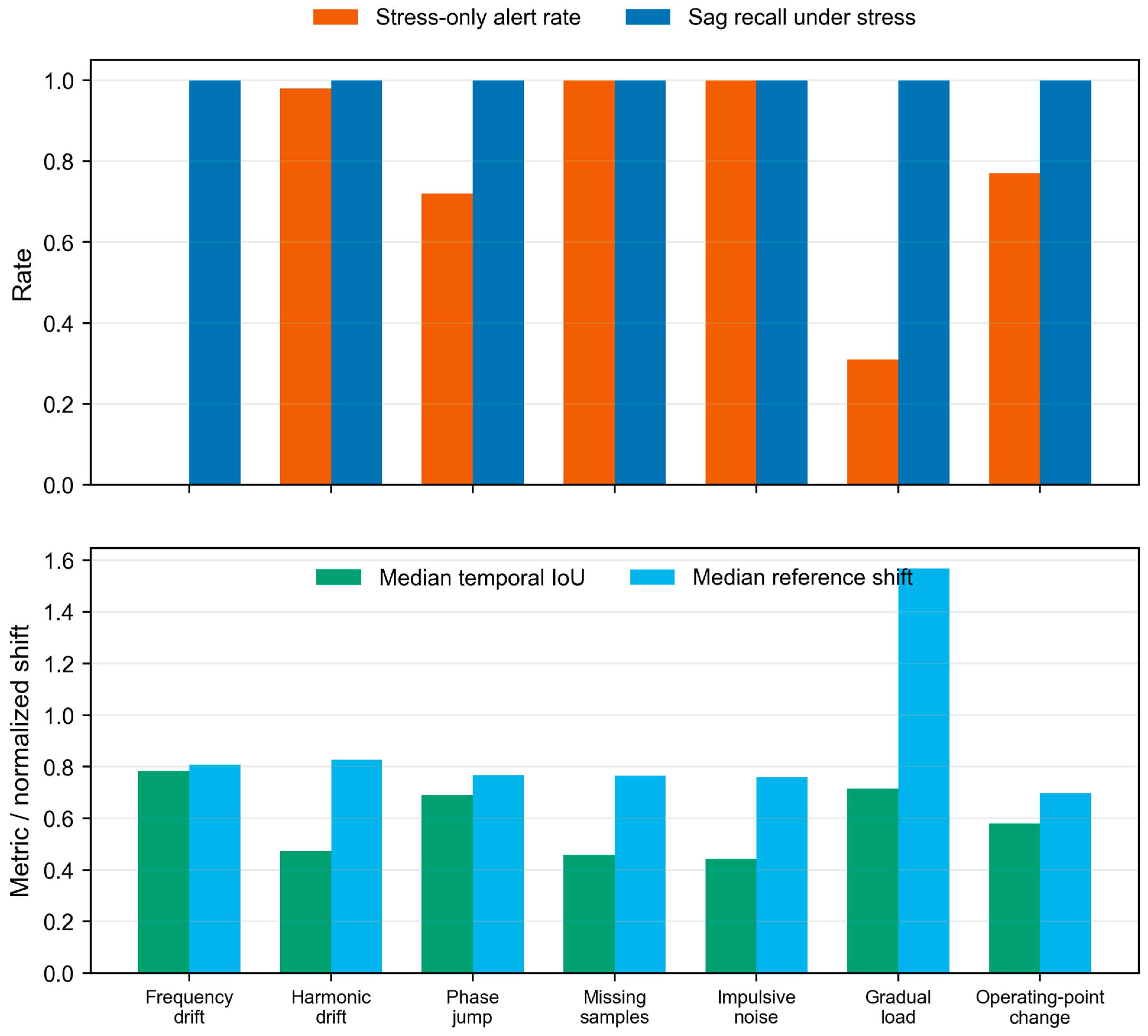
The extended robustness stress test examines seven conditions: frequency drift, harmonic background drift, phase jump, missing samples, impulsive measurement noise, gradual load change, and legitimate operating point step. For each condition, background samples containing only the stress factor and samples with a superimposed standard sag are generated (Figure 9). All detection settings follow the main experiment, and no recalibration is performed with the stress test results. Table 6 reports the background alarms, sag captures, tIoU, and final-state reference drift.

Figure 9. Alarms, sag captures, interval overlap, and normal reference drift under seven operating and measurement stress conditions.

Table 6. Extended robustness stress test.

Stress Condition	Background Realizations	Background Alarms	Superimposed Sags Captured	Median tIoU/%	Median Reference Shift
Frequency drift	100	0	100/100	78.43	0.808
Harmonic background drift	100	98	100/100	47.34	0.827
Phase jump	100	72	100/100	68.97	0.768
Missing samples	100	100	100/100	45.72	0.766
Impulsive measurement noise	100	100	100/100	44.20	0.759
Gradual load change	100	31	100/100	71.43	1.568
Legitimate operating point step	100	77	100/100	57.97	0.697

All superimposed sags are captured, but the harmonic background drift, missing samples, impulsive measurement noise, and legitimate operating point step themselves trigger alarms in 98, 100, 100, and 77 samples, respectively, indicating that the current scorer has a limited ability to distinguish non-event measurement changes. The median final-state reference drift of the gradual load condition is 1.568, which is the highest among the seven conditions.

5. Conclusions

This paper formulates online power quality anomaly capture as a combined pipeline of fixed feature standardization, an adaptive normal reference, causal similarity attention, and gated updating. The training partition fits the feature statistics and the reference using only normal windows, and the labeled validation partition is used to select the alarm threshold; the proposed method does not implement a Transformer trained with anomaly and boundary labels. On the test samples of this paper, the event-level precision, recall, and F1 are 91.93%, 91.11%, and 91.52%, respectively, the window-level F1 is 96.07%, and the median tIoU is 42.14%. The proposed method achieves the highest window-level recall and the highest event-level F1 among the seven methods, while its window-level F1 and tIoU are lower than those of the two learning baselines. The evidence therefore supports significantly higher detection sensitivity than other algorithms under the controlled disturbance repeated measurement protocol, rather than overall superiority, independent field generalization, or full-system real-time performance.

Appendix A.1. State Space, Completeness, and Self-Mapping

Let $d=15$ and take a finite truncation constant $K>0$ to define $\mathcal{X}={[-K,K]}^d$. On $\mathcal{X}$, the infinity norm metric $d_{\mathrm{\infty }}(p,p^{\prime })={∥p-p^{\prime }∥}_{\mathrm{\infty }}$ is adopted. $\mathcal{X}$ is a closed subset of the finite-dimensional Banach space $R^d$, and is therefore $(\mathcal{X},d_{\mathrm{\infty }})$ complete. The dimension-wise median of the training normal windows gives $p_0$; the bounded candidate $c_k=\mathrm{c}\mathrm{l}\mathrm{i}\mathrm{p}(z_k,-K,K)$ belongs to $\mathcal{X}$.

Let $q_k\in \{0,1\}$ denote the update gate, where $q_k=1$ indicates that the current window satisfies the update condition. The reference update in the implementation is uniformly written as

$$p_k=T_{c_k,q_k}(p_{k-1})=(1-q_k\alpha )p_{k-1}+q_k\alpha c_k,0<\alpha <1.$$

(A1)

When $q_k=1$, $T_{c_k,1}(p)$ is a convex combination of $p$ and $c_k$, so $T_{c_k,1}(\mathcal{X})\subseteq \mathcal{X}$; when $q_k=0$, $T_{c_k,0}(p)=p$, which also satisfies self-mapping. Therefore, as long as $p_0\in \mathcal{X}$, all $p_k$ remain in $\mathcal{X}$. The auxiliary scoring state and the FIFO token history are driven by time-varying windows and are not merged in this paper into a product space map claimed to share a common fixed point.

Appendix A.2. Contraction, Time-Varying Tracking, and Bounded Contamination Bounds

Proposition A1

(fixed candidate, update gate open). If $q_k=1$ and $c_k=c$ is fixed, then for any $p,p^{\prime }\in \mathcal{X}$,

$${∥T_{c,1}(p)-T_{c,1}(p^{\prime })∥}_{\mathrm{\infty }}=(1-\alpha ){∥p-p^{\prime }∥}_{\mathrm{\infty }}=\rho {∥p-p^{\prime }∥}_{\mathrm{\infty }},\rho =1-\alpha \in (0,1).$$

(A2)

Therefore, $T_{c,1}$ is a contraction on the complete space $\mathcal{X}$, and there exists a unique fixed point $p^{*}=c$ with ${∥p_k-c∥}_{\mathrm{\infty }}\le {\rho }^k{∥p_0-c∥}_{\mathrm{\infty }}$. If $q_k=0$, the map is the identity with Lipschitz constant 1, which is only non-expansive rather than strictly contractive. Consequently, the complete gated system under arbitrary switching sequences cannot be formulated as globally Banach-convergent.

Proposition A2

(tracking bound for time-varying candidates).  During m consecutive update-permitted steps, let $\rho =1-\alpha$ and define $e_k=p_k-c_k$; then

$${∥e_k∥}_{\mathrm{\infty }}\le {\rho }^m{∥e_{k-m}∥}_{\mathrm{\infty }}+\rho {\displaystyle {\sum }_{i=0}^{m-1}}{\rho }^i{∥c_{k-i}-c_{k-i-1}∥}_{\mathrm{\infty }}.$$

(A3)

The proof follows by recursion on $e_k=\rho (e_{k-1}+c_{k-1}-c_k)$, with repeated use of the triangle inequality. If the variation between adjacent candidates satisfies ${∥c_k-c_{k-1}∥}_{\mathrm{\infty }}\le \delta$, the asymptotic tracking error is bounded above by ${\displaystyle \frac{\rho \delta }{1-\rho }}$. This bound indicates that a smaller α suppresses fast contamination but increases the lag with respect to a slowly changing state. While the gate is closed, $p_k$ remains unchanged and Equation (A3) provides no error decay.

Proposition A3

(bounded contamination and constant bias). Compare the clean candidate $c_k$ and the contaminated candidate ${c^{\prime }}_k=c_k+b_k$ under the same gate sequence. If m consecutive update-permitted windows satisfy ${∥b_k∥}_{\mathrm{\infty }}\le B$, then

$${∥{p^{\prime }}_k-p_k∥}_{\mathrm{\infty }}\le \alpha B{\displaystyle {\sum }_{i=0}^{m-1}}{\rho }^i=B(1-{\rho }^m)\le B.$$

(A4)

If $b_k=b$ is constant, the reference bias is exactly $(1-{\rho }^m)b$. Bounded candidates give a finite worst-case coordinate difference bound. This conclusion is conditioned on the two trajectories having identical gate decisions; the actual score depends on the reference state, and contamination may change the gate decisions, in which case only the fact that both trajectories remain in $\mathcal{X}$ is guaranteed, and Equation (A4) cannot be claimed to remain tight.

References

- Pratticò, D.; Laganà, F.; Versaci, M.; Franković, D.; Jakoplić, A.; Vlahinić, S.; La Foresta, F. Enhancing Power Quality and Reducing Costs in Hybrid AC/DC Microgrids via Fuzzy EMS. Energies 2025, 18, 5985. [Google Scholar] [CrossRef] [Scilit]
- Barros, J.; Perez, E. Automatic Detection and Analysis of Voltage Events in Power Systems. IEEE Trans. Instrum. Meas. 2006, 55, 1487–1493. [Google Scholar] [CrossRef] [Scilit]
- Perez, E.; Barros, J. A Proposal for On-Line Detection and Classification of Voltage Events in Power Systems. IEEE Trans. Power Deliv. 2008, 23, 2132–2138. [Google Scholar] [CrossRef] [Scilit]
- Karimi, M.; Mokhtari, H.; Iravani, M.R. Wavelet Based On-Line Disturbance Detection for Power Quality Applications. IEEE Trans. Power Deliv. 2000, 15, 1212–1220. [Google Scholar] [CrossRef] [Scilit]
- Dash, P.K.; Panigrahi, B.K.; Panda, G. Power Quality Analysis Using S-Transform. IEEE Trans. Power Deliv. 2003, 18, 406–411. [Google Scholar] [CrossRef] [Scilit]
- Dash, P.K.; Panigrahi, B.K.; Sahoo, D.K.; Panda, G. Power Quality Disturbance Data Compression, Detection, and Classification Using Integrated Spline Wavelet and S-Transform. IEEE Trans. Power Deliv. 2003, 18, 595–600. [Google Scholar] [CrossRef] [Scilit]
- Mishra, S.; Bhende, C.N.; Panigrahi, B.K. Detection and Classification of Power Quality Disturbances Using S-Transform and Probabilistic Neural Network. IEEE Trans. Power Deliv. 2008, 23, 280–287. [Google Scholar] [CrossRef] [Scilit]
- Albalooshi, F.A.; Qader, M.R. Deep Learning Algorithm for Automatic Classification of Power Quality Disturbances. Appl. Sci. 2025, 15, 1442. [Google Scholar] [CrossRef] [Scilit]
- Iliadis, P.; Petridis, S.; Skembris, A.; Rakopoulos, D.; Kosmatopoulos, E. Physics-Informed Neural Networks for Enhanced State Estimation in Unbalanced Distribution Power Systems. Appl. Sci. 2025, 15, 7507. [Google Scholar] [CrossRef] [Scilit]
- Palomares-Salas, J.C.; Aguado-González, S.; Sierra-Fernández, J.M. Robustness of Machine Learning and Deep Learning Models for Power Quality Disturbance Classification: A Cross-Platform Analysis. Appl. Sci. 2025, 15, 10602. [Google Scholar] [CrossRef] [Scilit]
- Jiang, Z.; Ma, Z.; Shuai, Z. A Framework for Simultaneous Identification of Three-Phase Power Quality Events Based on Frame-Frequency Attention. IEEE Trans. Instrum. Meas. 2025, 74, 2553313. [Google Scholar] [CrossRef] [Scilit]
- Jian, X.; Cheng, X. PCTAR-Net: A Power Quality Composite Disturbances Classification Model for Variable Scenarios. Measurement 2025, 247, 116757. [Google Scholar] [CrossRef] [Scilit]
- Song, J.; Jiang, Q.; He, Z.; Wen, Z.; Peng, Z.; Hu, Z.; Wang, X.; Lu, S. Power Quality Disturbance Recognition Based on Lightweight Deep Neural Network Deployed in Edge Computing System. IEEE Sens. J. 2026, 26, 21243–21253. [Google Scholar] [CrossRef] [Scilit]
- Patrizi, G.; Garzon Alfonso, C.; Calandroni, L.; Bartolini, A.; Iturrino Garcia, C.; Paolucci, L.; Grasso, F.; Ciani, L. Anomaly Detection for Power Quality Analysis Using Smart Metering Systems. Sensors 2024, 24, 5807. [Google Scholar] [CrossRef] [Scilit] [PubMed]
- Wang, X.; Yao, Z.; Papaefthymiou, M. A real-time electrical load forecasting and unsupervised anomaly detection framework. Appl. Energy 2023, 330, 120279. [Google Scholar] [CrossRef] [Scilit]
- IEEE Std 1159-2019; IEEE Recommended Practice for Monitoring Electric Power Quality. IEEE Standard Association: Piscataway, NJ, USA, 2019.
- Machlev, R.; Chachkes, A.; Belikov, J.; Beck, Y.; Levron, Y. Open source dataset generator for power quality disturbances with deep-learning reference classifiers. Electr. Power Syst. Res. 2021, 195, 107152. [Google Scholar] [CrossRef] [Scilit]
- Laganà, F.; Pratticò, D.; Bibbò, L.; Pullano, S.A.; Calcagno, S. Integrated Fault Diagnosis in Grid-Connected PV Systems: Synergizing Infrared Thermography and Advanced Signal Processing. Appl. Sci. 2026, 16, 6036. [Google Scholar] [CrossRef] [Scilit]
- Hochreiter, S.; Schmidhuber, J. Long Short-Term Memory. Neural Comput. 1997, 9, 1735–1780. [Google Scholar] [CrossRef] [Scilit] [PubMed]
- Vaswani, A.; Shazeer, N.; Parmar, N.; Uszkoreit, J.; Jones, L.; Gomez, A.N.; Kaiser, L.; Polosukhin, I. Attention Is All You Need. In Proceedings of the Advances in Neural Information Processing Systems, Long Beach, CA, USA, 4–9 December 2017. [Google Scholar]
- Xu, J.; Wu, H.; Wang, J.; Long, M. Anomaly Transformer: Time Series Anomaly Detection with Association Discrepancy. In Proceedings of the International Conference on Learning Representations, Virtual, 25–29 April 2022. [Google Scholar]
- Tuli, S.; Casale, G.; Jennings, N.R. TranAD: Deep Transformer Networks for Anomaly Detection in Multivariate Time Series Data. In Proceedings of the VLDB Endowment, Sydney, Australia, 5–9 September 2022; Volume 15, pp. 1201–1214. [Google Scholar] [CrossRef] [Scilit]
- Ramsay, J.O.; Silverman, B.W. Functional Data Analysis, 2nd ed.; Springer: New York, NY, USA, 2005. [Google Scholar] [CrossRef] [Scilit]
- Zoubir, A.M.; Koivunen, V.; Chakhchoukh, Y.; Muma, M. Robust Estimation in Signal Processing: A Tutorial-Style Treatment of Fundamental Concepts. IEEE Signal Process. Mag. 2012, 29, 61–80. [Google Scholar] [CrossRef] [Scilit]
- Bai, S.; Kolter, J.Z.; Koltun, V. Deep Equilibrium Models. Adv. Neural Inf. Process. Syst. 2019, 32. [Google Scholar]
- Banach, S. Sur les operations dans les ensembles abstraits et leur application aux equations integrales. Fundam. Math. 1922, 3, 133–181. [Google Scholar] [CrossRef] [Scilit]
- Laganà, F. Design and Simulation-Based Validation of an Embedded Acquisition Architecture for In Situ PCB Integrity Monitoring in Biomedical Devices. Electronics 2026, 15, 833. [Google Scholar] [CrossRef] [Scilit]
- Sakurada, M.; Yairi, T. Anomaly Detection Using Autoencoders with Nonlinear Dimensionality Reduction. In Proceedings of the MLSDA 2014, Gold Coast, Australia, 2 December 2014; pp. 4–11. [Google Scholar] [CrossRef] [Scilit]
- Malhotra, P.; Vig, L.; Shroff, G.; Agarwal, P. Long Short Term Memory Networks for Anomaly Detection in Time Series. In Proceedings of the 23rd ESANN, Bruges, Belgium, 22–24 April 2015; pp. 89–94. [Google Scholar]
Disclaimer/Publisher’s Note: The statements, opinions and data contained in all publications are solely those of the individual author(s) and contributor(s) and not of MDPI and/or the editor(s). MDPI and/or the editor(s) disclaim responsibility for any injury to people or property resulting from any ideas, methods, instructions or products referred to in the content. |
© 2026 by the authors. Licensee MDPI, Basel, Switzerland. This article is an open access article distributed under the terms and conditions of the Creative Commons Attribution (CC BY) license.