Early Porosity Detection in High-Pressure Die Casting Using Explainable Multimodal Data Fusion

Abstract

Early and reliable detection of defects in the metal industry is crucial for improving quality, reducing costs and minimizing the environmental impact of manufacturing processes. In High-Pressure Die Casting (HPDC), porosity is one of the most severe defect types. This paper presents an explainable, multimodal approach to the early detection of porosity, which can be used as a preliminary step to reduce the number of parts requiring further, more time-consuming and expensive tests. Our work combines different data sources, such as machine sensor measurements, process time-series data and thermal images, to extract meaningful information and improve the final classification. The main classifier used is based on Fuzzy Cognitive Maps (FCMs), which provide a much higher interpretability of results and decisions, as well as of the model, compared to deep learning approaches. Building on our previous research, we have developed new feature extraction methods, classification approaches, and weight-selection strategies. Additionally, we investigated the DINOv2 foundation model for extracting features from thermal images and reducing the feature space using Principal Component Analysis (PCA). The experimental results show that the proposed approach improves defect detection performance compared to previous approaches and the HP-GAN algorithm without losing interpretability, allowing analysis of the relationship between input features and classification decisions. The proposed approach demonstrates how explainable artificial intelligence can support quality monitoring in real-life industrial use cases. Unfortunately, a performance advantage of the multimodal classifier over the strongest single-modality approach has not been demonstrated, and this will be further investigated as one of the future research directions.

1. Introduction

Modern industry is currently facing many problems, such as supply chain disruptions, rising energy costs, and a lack of resources. Therefore, it is crucial to optimize production processes in order to efficiently monitor and improve product quality and reduce the number of defective parts and scrap [1,2,3].

In High-Pressure Die Casting (HPDC), many factors influence the quality of the final part. Examples include temperature-related factors (e.g., surface or melt temperature), process parameters, or post-demolding treatment, which can affect the final properties of the part. Defects occurring in the production process can be categorized as either surface or internal defects [4]. Common surface defects include cold flows, ejection marks, and incomplete filling. The most common internal defects, which have the greatest impact on the final part quality, are different types of porosity, such as shrinkage or gas porosity. Shrinkage porosity forms during solidification when the liquid metal cannot compensate for the volume contraction associated with solidification [5]. It forms when the thermal conditions or process parameters are not appropriate, e.g., melt temperature or pressure [5]. Gas porosity is associated with gas and air entrapment during the filling and injection stages [6,7]. However, the mechanisms are not completely independent and can also influence the formation of shrinkage porosity [8]. Additionally, porosity may appear in different populations with distinct sizes, distributions, and characteristics [9,10].

Surface defects can be detected by visual inspection, either by a human or automatically. Internal defects are more challenging, as their presence is not visible externally. For such defects, destructive and non-destructive techniques are used. Common destructive techniques include metallographic cuts [11], tensile testing [12], or fractographic analysis [13]. When destructive tests are performed, the part cannot be used anymore; thus, non-destructive methods are preferred whenever applicable. Common non-destructive methods include leakage tests [14], X-ray radiography [15,16], and computed tomography (CT) [16,17]. However, despite their effectiveness, these methods are costly and often cannot be easily integrated into the production line. Therefore, there is a need for preliminary, in-line quality assessment to reduce the number of parts that must be investigated more thoroughly. In this area, studies have shown that analysis of thermal images [18] and process data [19,20] can be used for preliminary quality assessment and defect prediction.

Defect detection using computer-supported methods in the metal industry has been studied for many years. Many studies focus only on surface defects, such as inclusions, different types of stains, cracks, pits, or scratches [21]. Both classical machine learning [21] and deep learning [21,22] methods are used. However, when internal defects must be detected, fewer methods are available, with most approaches being based on the aforementioned non-destructive testing techniques. For example, the following approaches have been successfully applied to processes other than HPDC: processing images from XCT with postprocessing to extract porosity [23], analysis of acoustic spectroscopy signals using deep learning [24], and processing of EMD spectrometer signals using a modified SVM and genetic algorithm approach [25].

In the case of High-Pressure Die Casting, many of these methods can also be applied, with modifications tailored to process characteristics. Both classical machine learning (ML) and deep learning (DL) methods can be used for detecting different types of defects and process quality monitoring. Examples of ML methods used in recent studies include Random Forests [20,26], Support Vector Machines [20], and XGBoost and CatBoost classifiers [19]. Machine learning methods provide good results when the features extracted from the data are meaningful [27]. Among DL methods (especially for images), Convolutional Neural Networks (CNNs) [27], ResNet50 [28], or YOLOv5 [27] are often used to learn high-level features and detect defects [27]. For example, Faster R-CNN or YOLOv5 can be used to detect surface defects [29]. Another approach to process quality prediction is using simulations, which can be particularly effective for misruns or cold shuts [30]. For detecting internal defects, a data-fusion approach can be used [26], merging data from Internet of Things (IoT) sensors and simulations, and analyzing them using a Decision Tree, Random Forest, Artificial Neural Network, or Support Vector Machine. However, the work provides limited information about validation on real production data and does not include additional vision-based data. Additionally, prediction quality may depend on the parameter settings represented in the typical good and bad samples from which the model learned, potentially making it less effective in atypical situations. Another example of sensor-fusion-based approaches is [31], which uses thermal images and sensor readouts, similarly to our work. The authors used the HP-GAN (Hypothesis Pruning Generative Adversarial Network) architecture, which is based on CNN and GAN networks, and showed that such an approach can provide highly effective defect prediction. However, this solution has limitations that may restrict broader adoption, including missing information about the datasets used for training and testing, limited details on the evaluation methodology and performance measurements, and limited scalability.

Our paper focuses on the use of Fuzzy Cognitive Maps (FCMs) for multimodal data fusion and classification. Fuzzy Cognitive Maps have been used successfully in many areas, providing explainable insight into classification [32] or forecasting processes, with a graph-like structure [33]. For preprocessing and feature extraction, models such as VGG-16 [34] or Vision Transformers [35] can be used. For classification, the output may be binary [33] or multi-label [35].

The main contributions of our paper are as follows:

• A novel approach for porosity detection in HPDC, based on our previous work [36], with many extensions; the main differences between the previous work and this work are shown in Table 1.
• An analysis of the informativeness of thermal images, process data readouts, and time-series data for the final prediction.
• An analysis of how a foundation model can improve feature extraction for thermal images.
• An analysis of how feature-space reduction influences the results.
• An analysis of how different training algorithms influence the results.
• An analysis and comparison of a data-fusion approach with single-data-source approaches.
• An analysis of model complexity for different approaches.
• Improved explainability of the model and its decisions.
• Performance comparisons with the HP-GAN algorithm [31].

Table 1. Comparison between the previous FCM-based porosity classifier [36] and the framework proposed in this work. Performance values come from different datasets and metric sets and are therefore not directly comparable.

Aspect	Previous Study [36]	This Work
Data sources	Machine header data (structured sensor readouts) and thermal images (before/after spraying)	Three modalities: header data, thermal images, and time-series profiles
Dataset	Two separate balanced datasets, one per data source, plus a fused balanced dataset	Single combined balanced dataset: 200 OK/183 porosity parts; 305 train/78 test;
Feature extraction	Dedicated DNN extractors (U-Net, ResNet50, U-Net + ResNet50; TabNet, LightGBM, MLP); variance reduction, PCA, GA	Dedicated DNN, DINOv2 (no training), DINOv2 (with Siamese training) for thermal images; DTW- and statistics-based features for time-series data; PCA
Model/fusion	FCM per data source; fused header + thermal FCM variants	Two-stage, multimodal, and multi-input FCMs (with and without centroids); GA for concept and weight selection; systematic ablation across different variants
Evaluation	Train/test split; AUC, MCC, balanced accuracy, F1, recall per class	Unified test set plus 5-fold cross-validation for selected models; confusion matrices; MCC-focused ablation

2. Materials and Methods

2.1. Data Sources and Features

During the High-Pressure Die Casting process, various types of data can be captured, such as information logged by the machine, external measurements, or images. These data can contain information that is useful for quality assessment and defect prediction/detection. Therefore, we recorded the following data types in the project:

• Numerical sensor readout data;
• Time-series data;
• Thermal images (before and after spraying).

During production, the process consists of multiple stages, and in HPDC it typically takes 15–40 s to produce a part. During that time, the different modalities are available as follows:

• Thermal images are taken before and after spraying (which is performed at the beginning of the process) for each cast part;
• Time-series data are collected throughout the process;
• Header data are available after the process is completed.

The final decision about the part quality using the proposed solution can be made directly after the casting cycle is finished—for example, when the part is removed from the mold. Therefore, the approach can be used in-line in a real industrial use case.

Since each data type has a different source and characteristics, we processed them using different methods to extract informative features for the classifiers.

2.1.1. Numerical Sensor Features (Header Data)

Numerical sensor values are the simplest features for further processing by classifiers because they can be easily transformed into feature vectors and used directly as inputs by most classifiers. However, since each sensor may have a different value range, it is recommended to normalize the data to obtain values within the range $[0,1]$. The numerical sensor feature vector can be defined as follows:

$${\mathbf{x}}^n=(x_1,x_2,\dots ,x_n),x_i^n\in [0,1]$$

(1)

In High-Pressure Die Casting, this type of data is often referred to as header data.

2.1.2. Sensor Time-Series Feature Extraction (Profile Data)

Time-series data are more difficult to use with standard classifiers because they contain numerical sensor values sampled at multiple time points. Therefore, to convert them into a single feature vector, they require additional processing. In our research, we focused on two approaches: (i) extracting statistical and frequency-domain features, and (ii) Dynamic Time Warping. In High-Pressure Die Casting, this type of data is often referred to as profile data or profiles.

Statistical and Frequency Features:

One approach to feature extraction from time-series data is to compute statistical features across all time points for each sensor. In our research, we computed the following characteristics: root mean square, peak-to-peak (maximum–minimum), crest factor, kurtosis, entropy, energy, power, mean, standard deviation, absolute mean of discrete difference, zero-crossing rate, autocorrelation, and interquartile range.

Other important characteristics are based on the frequency domain. In our research, we used the following: dominant frequency, power spectral density, spectral centroid, spectral spread, and spectral rolloff.

In addition to statistical and frequency-domain features, we computed the following: trend slope and normalized time to maximum and minimum, which may provide additional information for the HPDC process.

The statistical and frequency features can be summarized as follows:

$${\mathbf{x}}^{\left(ts\right)}=\left(f_{\mathrm{stat}},f_{\mathrm{dom}},P_{\mathrm{PSD}},C_{\mathrm{spec}},S_{\mathrm{spec}},R_{\mathrm{roll}},{\beta }_{\mathrm{trend}},t_{\max },t_{\min }\right),x_i^{\left(ts\right)}\in [0,1],i=1,\dots ,8$$

(2)

where

• $f_{\mathrm{stat}}$—Statistical features component, which consists of root mean square, peak-to-peak (maximum − minimum), crest factor, kurtosis, entropy, energy, power, mean, standard deviation and absolute mean of discrete difference, zero-crossing rate, autocorrelation, and interquartile range;
• $f_{\mathrm{dom}}$—Dominant frequency;
• $P_{\mathrm{PSD}}$—Power spectral density;
• $C_{\mathrm{spec}}$—Spectral centroid;
• $S_{\mathrm{spec}}$—Spectral spread;
• $R_{\mathrm{roll}}$—Spectral rolloff;
• ${\beta }_{\mathrm{trend}}$—Trend slope;
• $t_{\max },t_{\min }\in [0,1]$—Normalized time indices of maximum and minimum values.

Dynamic Time Warping (DTW):

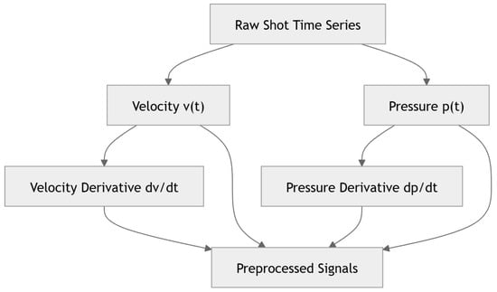
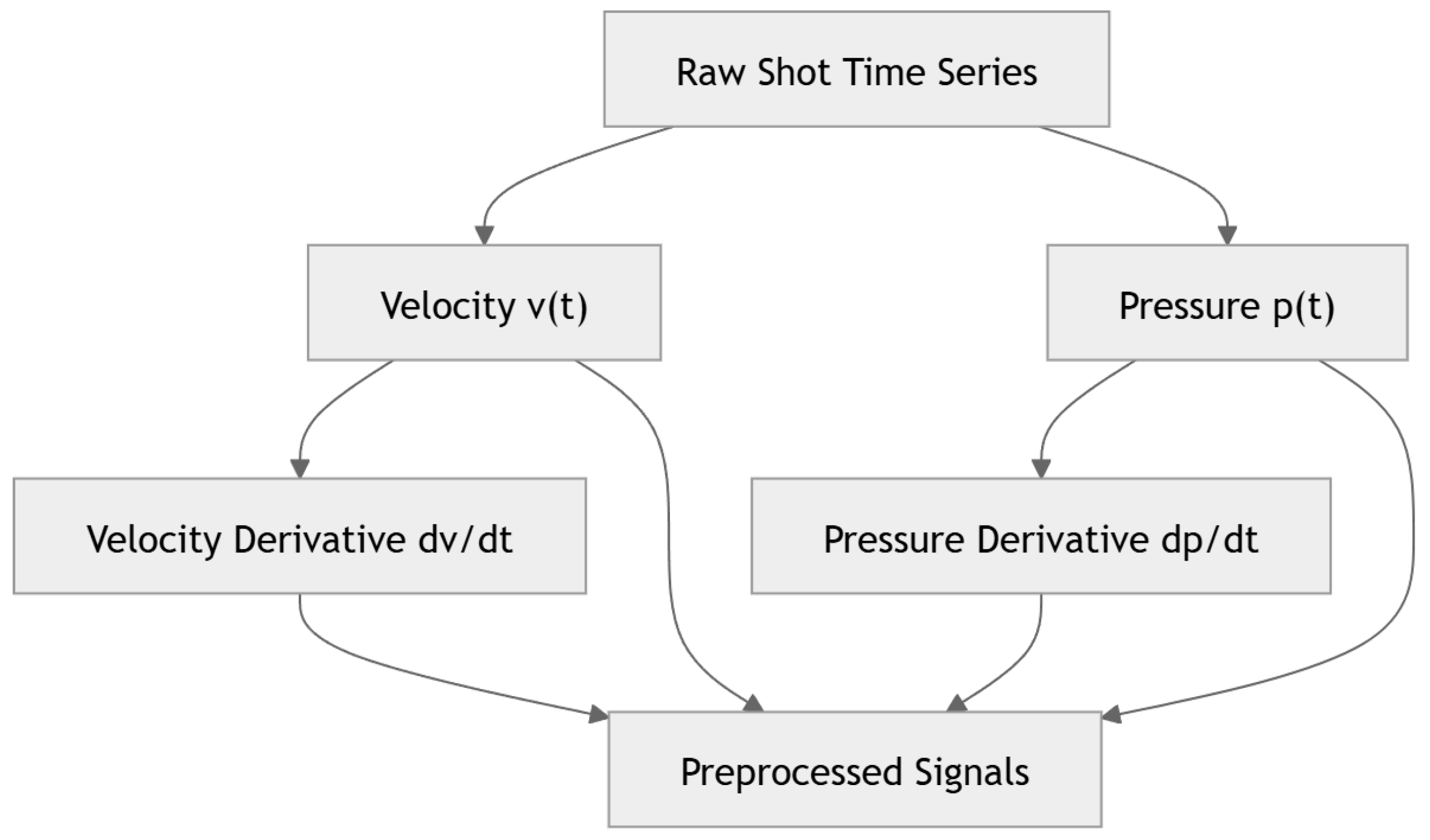
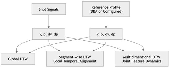
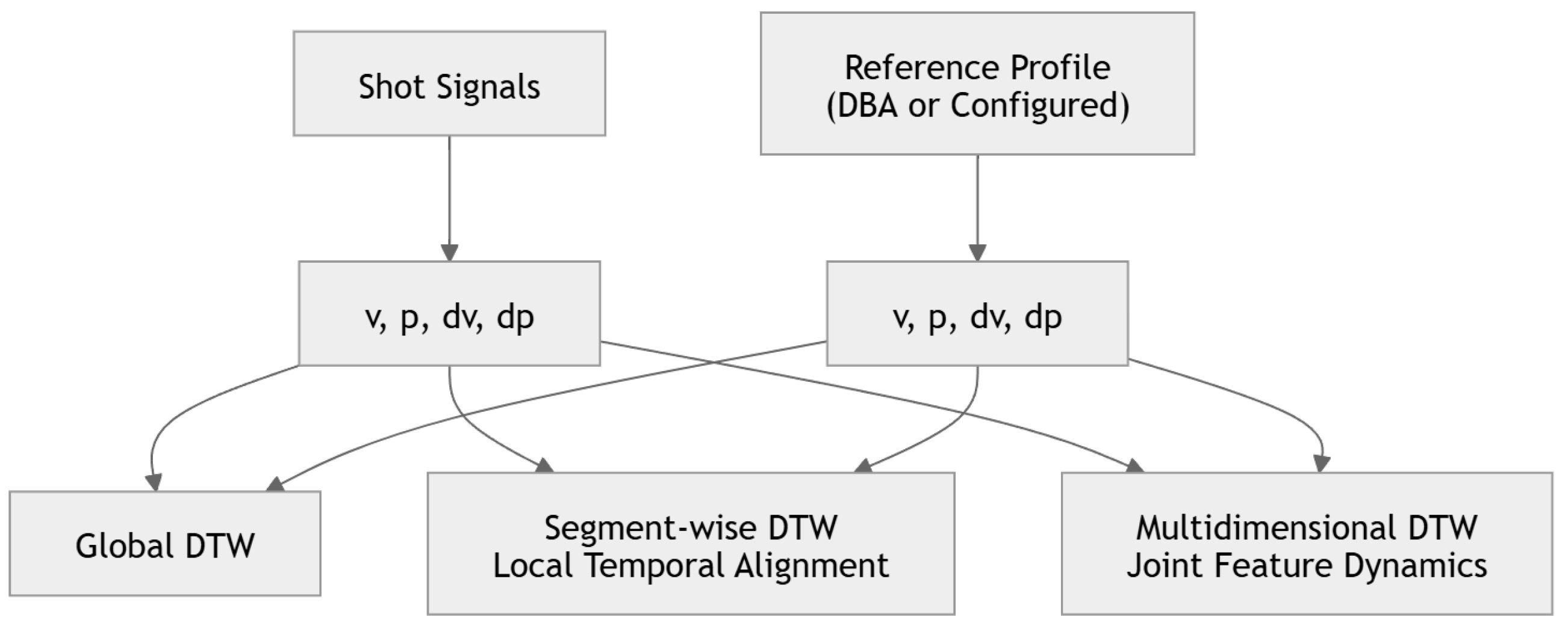
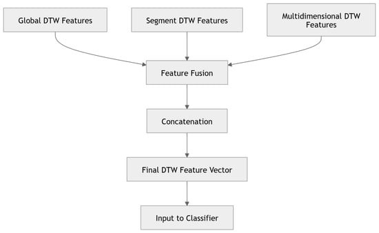
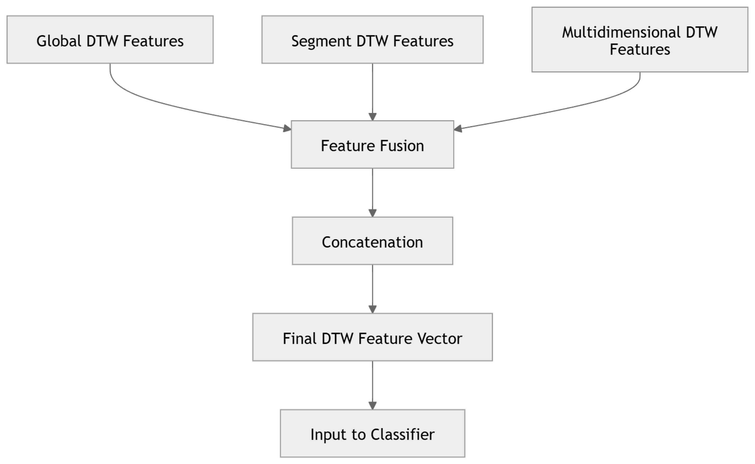
Another approach for analyzing time-series data is Dynamic Time Warping (DTW [37]). DTW aligns and compares two time series based on their shape. In our implementation, we compare each shot with a reference profile (computed using DTW Barycenter Averaging (DBA)) and then construct features from the alignment [38]. The general idea can be described in three steps: preprocessing (Figure 1), DTW alignment (Figure 2), and feature construction (Figure 3).

Figure 1. Overview of signal preprocessing for the Dynamic Time Warping feature extractor. Raw-shot time-series signals are used to extract velocity and pressure components, followed by computation of their derivatives.

Figure 2. Overview of the Dynamic Time Warping alignment. As an input, shot signals and reference profiles are used, and then ($v,p,dv,dp$) parameters are extracted from both of them. Finally, they are used to create three alignments: global DTW, segment-wise DTW for local temporal alignment, and multidimensional DTW for joint feature dynamics.

Figure 3. Final feature vector construction in the Dynamic Time Warping feature extractor. Global, segment, and multidimensional DTW features are merged using feature fusion and concatenation, creating one feature vector.

The DTW-based comparison of the analyzed signal to the reference signal can be defined as follows:

$$D_{\mathrm{DTW}}(\mathbf{x},\mathbf{r})=\underset{\pi \in \mathrm{\Pi }}{\min }\sum _{(i,j)\in \pi }∥x_i-r_j∥$$

(3)

where

• $\mathbf{x}=(x_1,\dots ,x_n)$—Analyzed signal;
• $\mathbf{r}=(r_1,\dots ,r_m)$—Reference signal;
• $\pi$—Warping path;
• $\mathrm{\Pi }$—The set of all possible paths.

The DTW distance and the warping path are used to construct a set of features that describe the similarity between the reference and analyzed signals. In general, the DTW-based feature set can be defined as follows:

$${\mathbf{x}}^{\left(\mathrm{dtw}\right)}=\left(f_1(\mathbf{x},\mathbf{r}),f_2(\mathbf{x},\mathbf{r}),\dots ,f_k(\mathbf{x},\mathbf{r})\right),{\mathbf{x}}^{\left(\mathrm{dtw}\right)}\in {[0,1]}^k$$

(4)

In our research, for each segment s, the following quantities are calculated:

$${\mathbf{f}}_s=\left(f_{s,\mathrm{sub}},f_{s,\mathrm{pos}},f_{s,\mathrm{neg}},f_{s,\mathrm{stretch}}\right)$$

(5)

where

• $f_{s,\mathrm{sub}}$—DTW-based deviation score within the segment;
• $f_{s,\mathrm{pos}}$ and $f_{s,\mathrm{neg}}$—Mean positive and negative deviations between the analyzed and reference signals along the DTW path;
• $f_{s,\mathrm{stretch}}$—Relative temporal stretching of the analyzed signal with respect to the reference signal within the segment.

2.1.3. Image Feature Extraction

There are many approaches to extracting features from images. Recently, Generative Adversarial Networks (GANs) and foundation models (e.g., the DINO family) have become increasingly popular. In our research, we use two thermal images of the mold for each casted part (before and after spraying), since they can contain useful information about thermal behavior and changes [36]. For this reason, we investigated three approaches:

• A neural network architecture based on U-Net, ResNet, and GAN, trained end to end on images from the dataset;
• DINOv2 as a feature extractor for both images, without fine-tuning;
• A DINOv2 Siamese-inspired architecture, using a pretrained DINOv2 model and a trained fully connected layer to improve performance.

U-Net + ResNet + GAN:

The proposed model architecture combines different block types to improve learning of the details and differences between the images before and after spraying. The blocks are as follows:

• U-Net-based encoder blocks;
• ResNet50 blocks;
• GAN discriminator blocks.

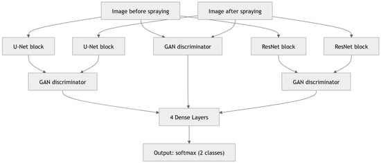
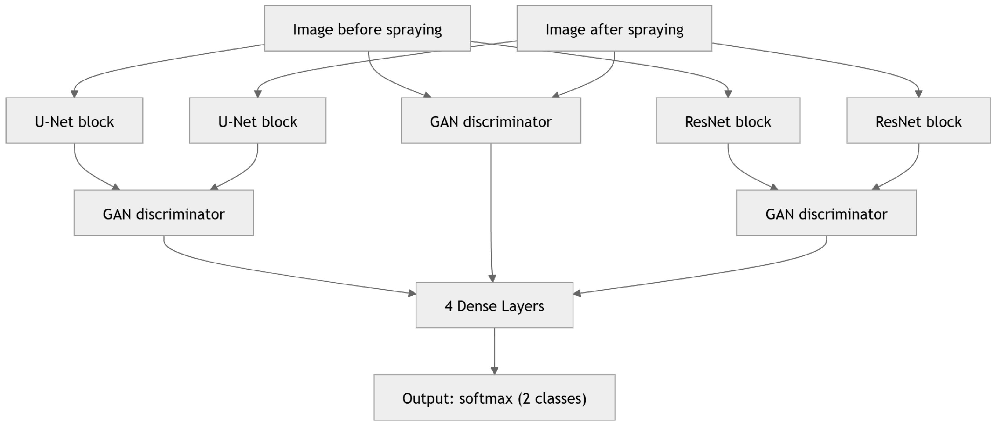
As shown in Figure 4, both images are processed separately by the U-Net and ResNet blocks. The output of each block type is then processed by a separate GAN discriminator. Additionally, the input images are processed by an additional GAN discriminator block. Finally, all discriminator outputs are concatenated and processed by four dense (fully connected) layers. During inference, the final layers are removed to extract a 256-dimensional embedding vector.

Figure 4. Architecture of the thermal image feature extractor. Images before and after spraying are processed through three parallel branches involving U-Net blocks, ResNet blocks, and GAN discriminators. Next, extracted features are aggregated by the four dense layers, producing the final binary output.

The final feature vector can be defined as follows:

$${\mathbf{x}}^{imgURG}=(x_1,x_2,\dots ,x_{256}),x_i^{imgURG}\in [0,1]$$

(6)

DINOv2 Model:

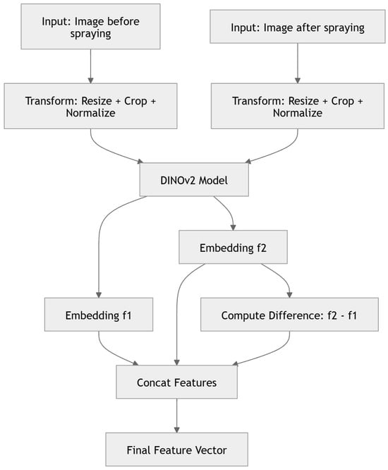
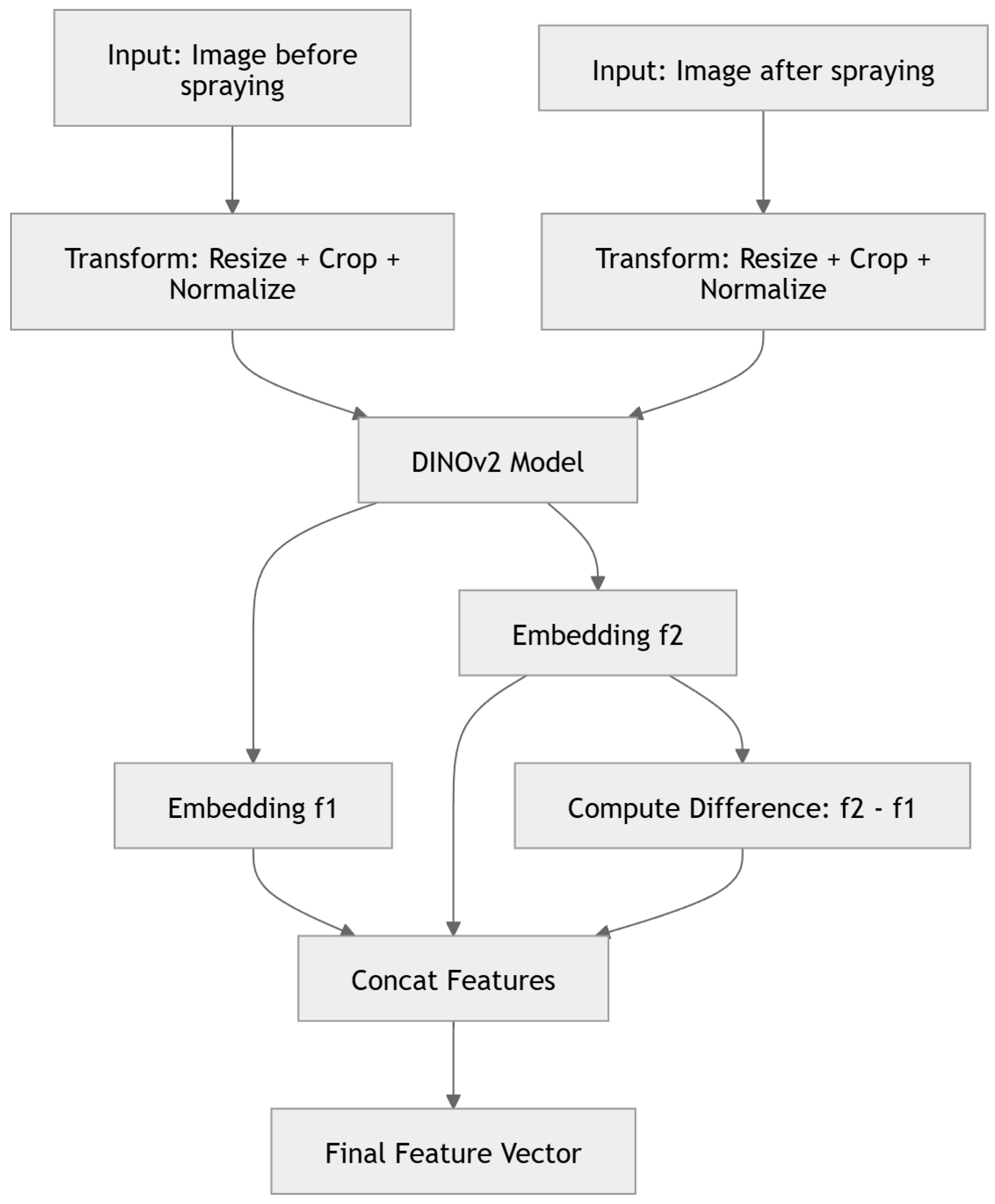
Another approach that we considered was using the DINOv2 model [39] as a feature extractor for both input images, without fine-tuning. The process of creating the feature vector is illustrated in Figure 5. The model extracts embeddings for the images separately ($f_1$ and $f_2$):

$${\mathbf{f}}_1=\varphi \left({\mathbf{I}}_1\right),{\mathbf{f}}_2=\varphi \left({\mathbf{I}}_2\right)$$

(7)

where $\varphi \left({\mathbf{I}}_i\right)$ denotes DINOv2 embeddings for the i-th image. We then compute their difference:

$$\Delta \mathbf{f}={\mathbf{f}}_2-{\mathbf{f}}_1$$

(8)

Figure 5. Architecture of the DINOv2-based thermal image feature extractor. Thermal images before and after spraying are resized, cropped, and normalized and then processed by DINOv2 to generate embeddings ($f_1$ and $f_2$). Additionally, their difference is computed and concatenated with $f_1$ and $f_2$ to form the final feature vector.

Finally, we concatenate them into one feature vector:

$${\mathbf{x}}^{\left(\mathrm{D}\right)}=\left[{\mathbf{f}}_1,{\mathbf{f}}_2,\Delta \mathbf{f}\right]$$

(9)

DINOv2 Siamese Model:

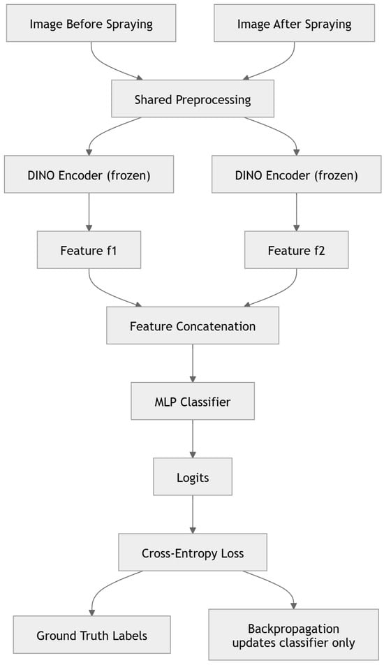
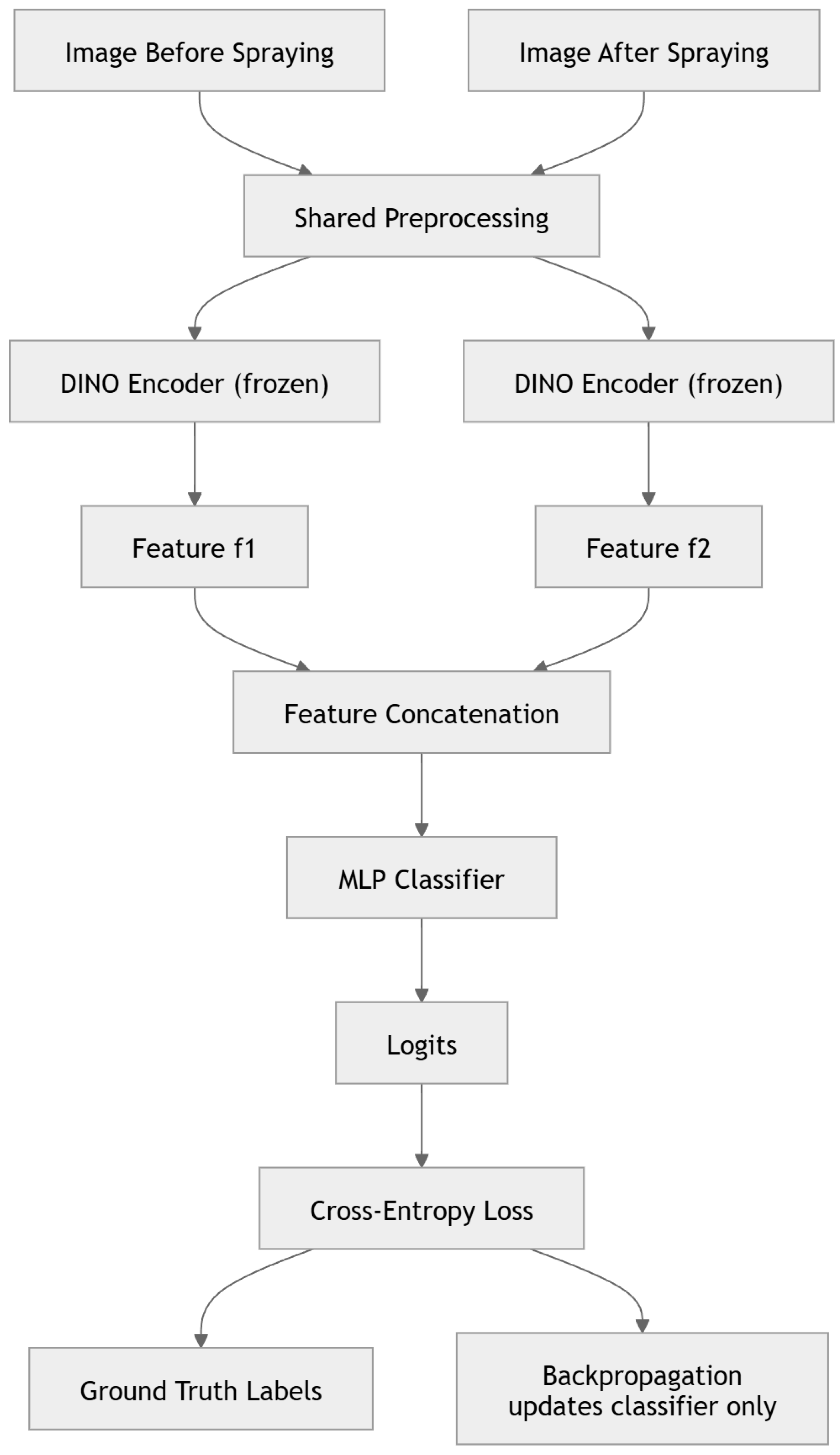
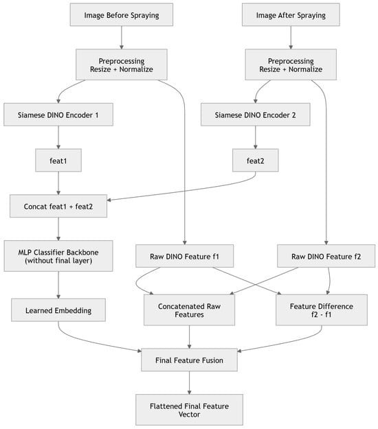
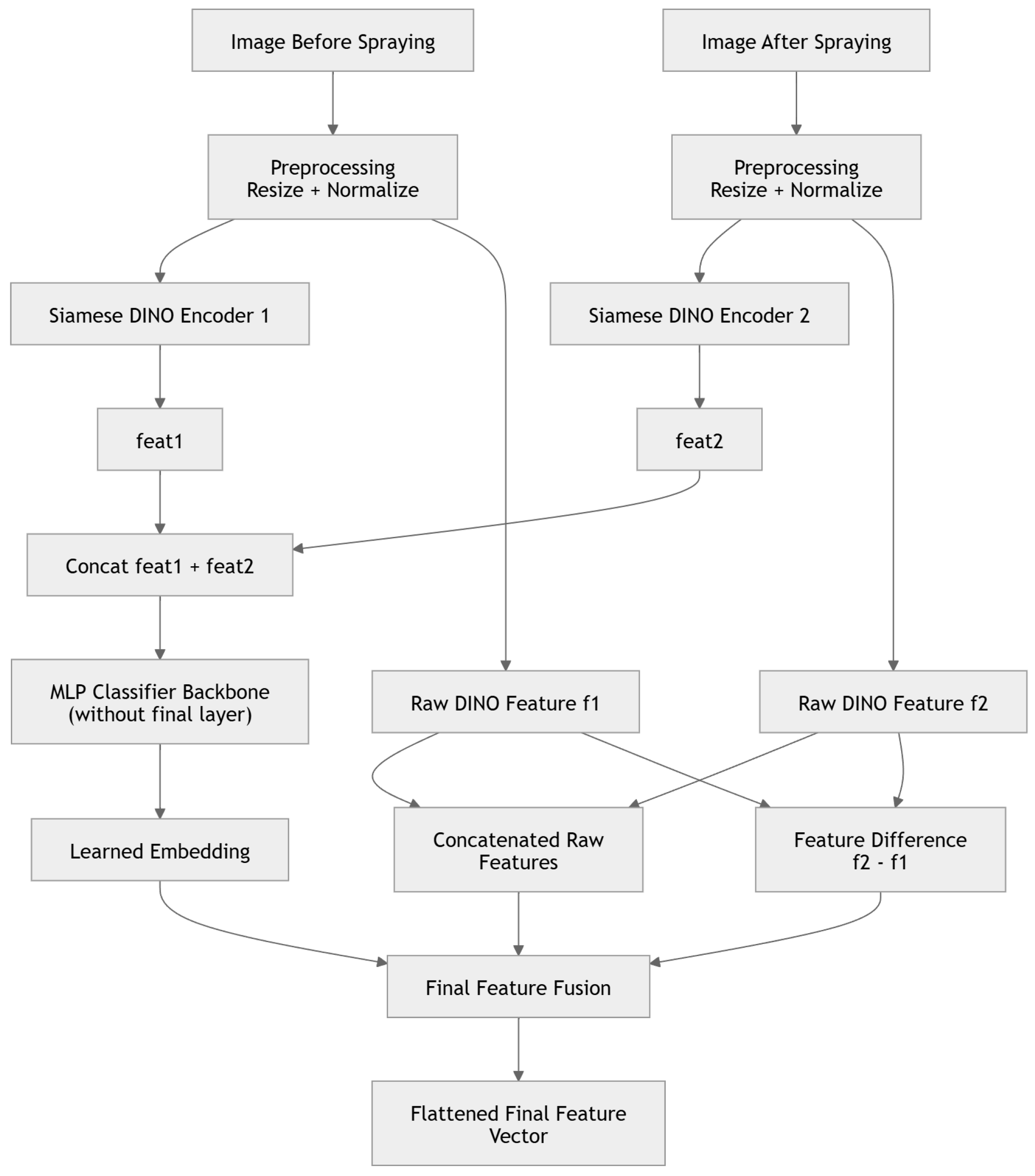
The final method of extracting features from images is based on a Siamese network that uses DINOv2 models as branches for the before- and after-spraying images. Training is similar to other Siamese networks: for each image, DINOv2 embeddings are computed, concatenated, and processed by an MLP classifier. Cross-entropy loss is then used to compare predictions with the ground-truth label (“OK” or “Porosity”). Backpropagation updates the classifier only, while the DINOv2 weights remain frozen. An overview of the training process is provided in Figure 6. During inference, the Siamese network with the last layer removed is used to compute the embedding $f_s$. Additionally, it is concatenated with the same embeddings as in the previous DINOv2 approach to prepare the final feature vector:

$${\mathbf{x}}^{\left(\mathrm{DS}\right)}=\left[{\mathbf{f}}_s,{\mathbf{f}}_1,{\mathbf{f}}_2,\Delta \mathbf{f}\right]$$

(10)

Figure 6. An overview of the thermal images DINOv2 Siamese feature extractor training. The architecture incorporates frozen DINO encoders for feature extraction ($f_1$ and $f_2$) from thermal images, followed by feature concatenation, an MLP classifier, and cross-entropy loss calculation where backpropagation updates the classifier only.

The overview of feature extraction is shown in Figure 7.

Figure 7. DINOv2 Siamese feature extractor overview, which illustrates how the thermal images are transformed into the final feature vector, using different blocks.

2.2. Classifiers

In our research, we evaluated various classifiers based on Fuzzy Cognitive Maps, using different weight-calculation algorithms and reference approaches, including maximization, XGBoost, and a perceptron.

2.2.1. Fuzzy Cognitive Map

Fuzzy Cognitive Maps (FCMs) were introduced by Kosko [40] in 1986 as a form of knowledge representation and decision-making. An FCM can be defined as a fuzzy directed graph that incorporates concepts from neural network architectures and their behavior. Nodes represent concepts in the analysis, and directed edges are assigned weights that represent relationships between concepts. In classification use cases, nodes are most often divided into two types: regular concepts, and concepts dedicated to the final classification. As with classical neural network architectures (e.g., the perceptron), there are two stages to creating the model: selecting the weights (training), and performing inference. Different strategies may be used for weight selection, including human expert input or computer algorithms based on centroids, gradient descent, or genetic algorithms. The inference phase initializes the concepts using an initial vector and updates their values with each iteration until the map converges or an iteration limit is reached. Kosko defined the classical concept update algorithm [40] during inference as follows:

$$X_i(t+1)=f\left({\displaystyle \sum _{j=1,j\ne i}^n}{w}_{j,i}{X}_j\left(t\right)\right),i,j=1,\dots ,n$$

(11)

where

• $X_i\left(t\right)$—The i-th concept value;
• t—Iteration index;
• $w_{j,i}$—Weight of the relationship from concept j to concept i;
• n—Total number of concepts;
• $f\left(x\right)$—Activation function.

As shown in the inference rule, the activation function is used to normalize the updated concept value to the range $[0,1]$ [41]. The most commonly used activation function is the sigmoidal function.

In our research, we considered multiple versions of FCMs, including centroid-based feature transformation into concept values (as described by Tziolas et al. [33]) and a classical approach that uses features directly as concept values.

The centroid-based feature transformation is based on clustering the features during training and calculating distances to the clusters’ centroids. Fuzzy sets are then created from these distances, and the final weights are calculated [33]. During inference, distances between the features and the centroids are computed, and the final state is obtained using the Kosko inference rule.

The classical approach uses the elements of the feature vector as consecutive concepts and updates these values using Equation (11).

Since our research focuses on multimodal data sources from a factory (process data, time-series data, and thermal images), we analyze how these can be processed using an FCM. We consider the following approaches:

• Separate FCMs for each data type (referred to later as separate-data-type FCMs);
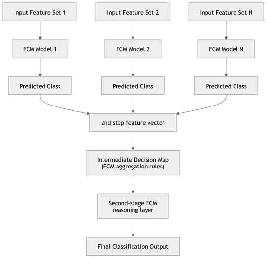
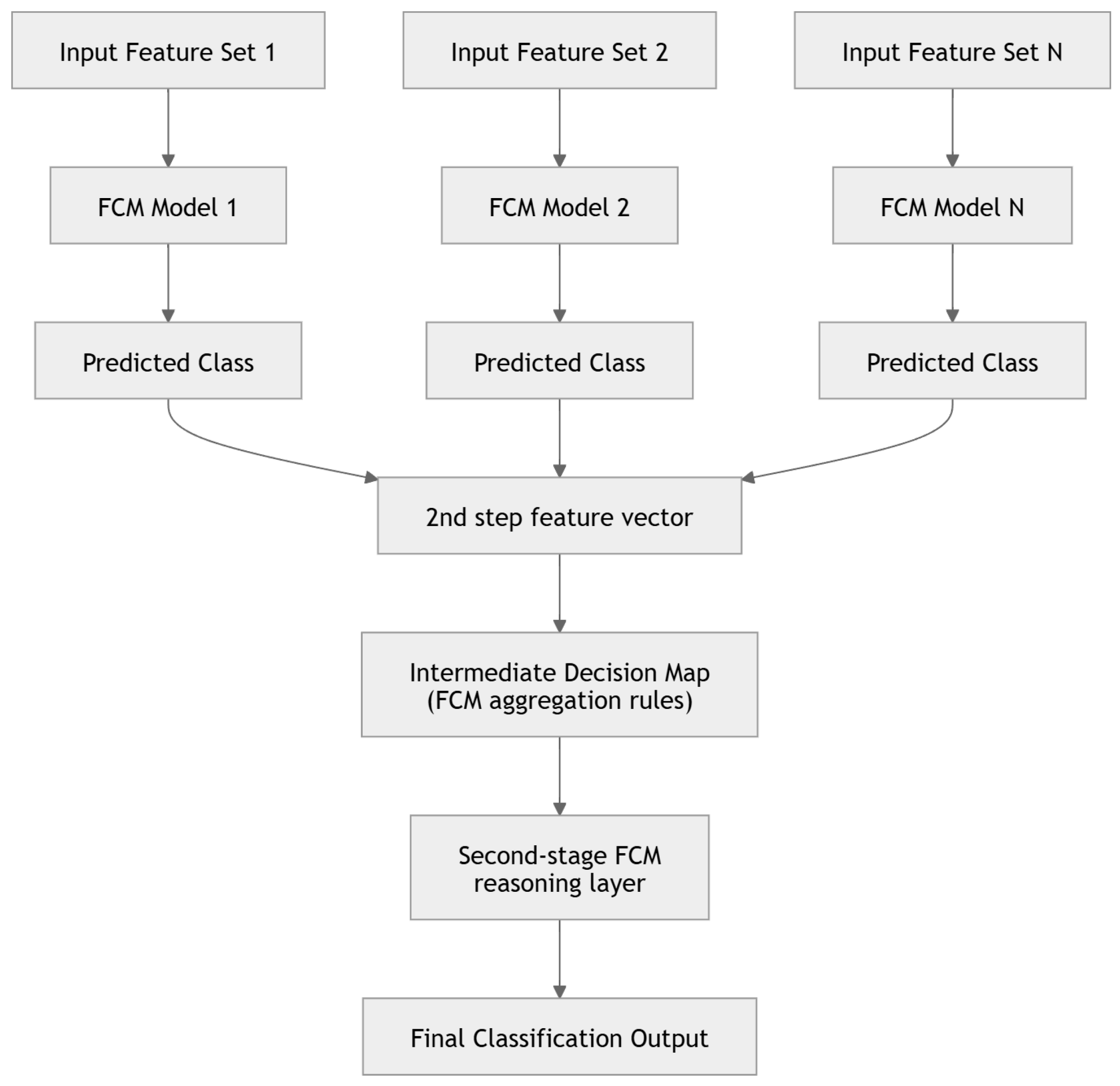
• Outputs from separate FCMs used as inputs to another FCM that performs voting and produces the final classification (referred to later as a 2-stage FCM);
• A single FCM with multiple data-type inputs (referred to later as a multimodal FCM).

When concepts come from different data sources (e.g., in 2-stage and multimodal FCMs), the relationships between them can be modeled in two ways:

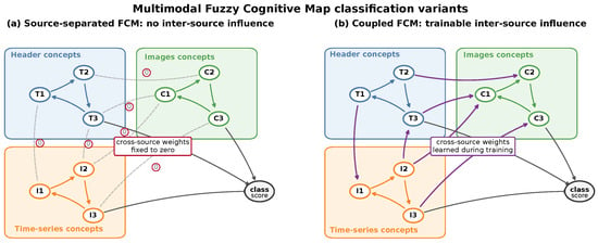
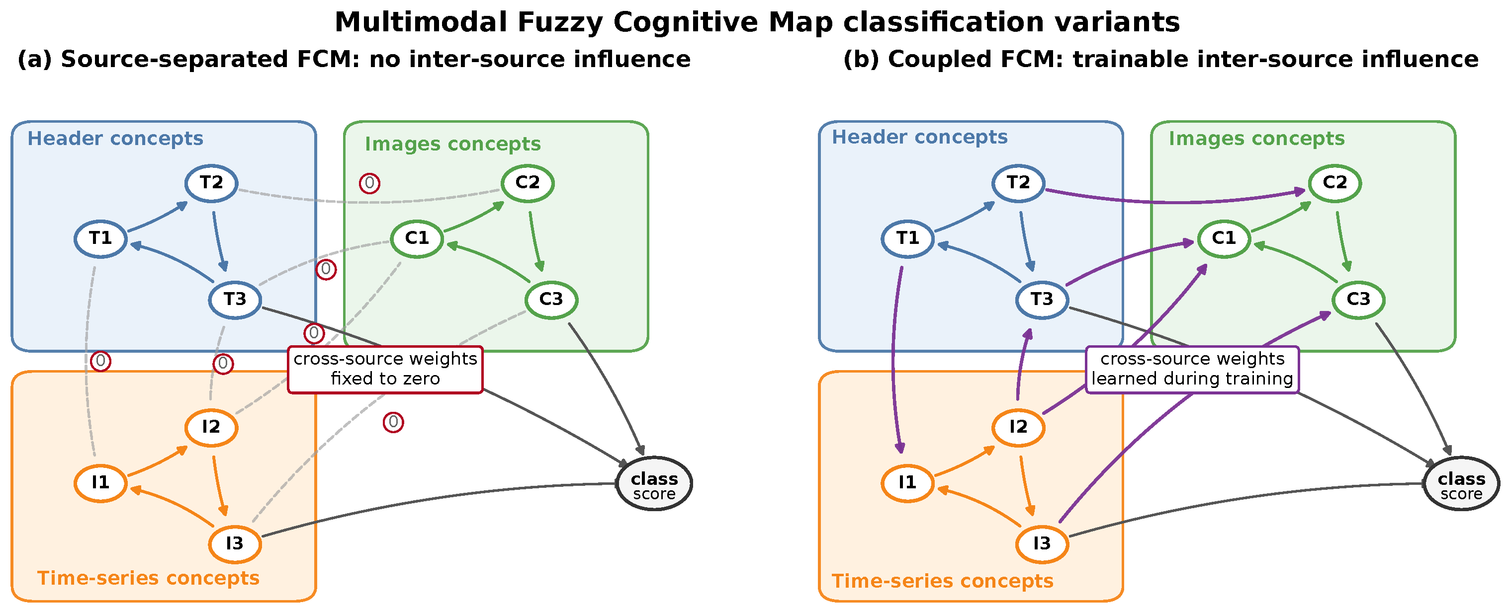
• Weights between concepts from different data sources are always set to 0 (Figure 8a);
• Weights between concepts from different data sources can be set during training (Figure 8b).

Figure 8. An overview of the two versions of the multimodal Fuzzy Cognitive Map: (a) weights between concepts from different data sources are always set to zero; (b) weights between concepts from different data sources can be set during training.

These two versions model different behaviors of the FCM: In the first type, all data sources are processed separately and only affect the output class concepts. In the second type, all concepts can influence each other; for example, a concept based on header data can influence a concept based on image data. In some cases, this may improve the performance of certain concepts; however, we did not make any assumptions prior to conducting the tests.

To analyze which structure and training algorithm are most suitable for our use case, we examined the following training algorithms:

• Centroids-Based FCM:

  –

  Centroids-Based Initial Approach: The general idea is based on [33]. In this algorithm, all features are clustered using the K-means algorithm, and fuzzy similarity measures are used to define causal relationships.

  –

  Gradient Descent: weight calculation is performed using gradient descent and backpropagation, based on [42].

  –

  Particle Swarm Optimization: Described by Papageorgiou et al. [43]; a swarm-intelligence algorithm is used to set the weights between concepts.

  –

  Active Hebbian Learning: Based on [44]; an active Hebbian principle is applied to set weights between concepts based on their final activation values.

  –

  Differential Hebbian Learning: Described in [45]; uses an improved method proposed by Kosko [46].

  –

  Simulated Annealing: Implemented using the classical approach from [47]; starts from randomly chosen weights and iteratively updates them, accepting better solutions while occasionally accepting worse ones based on the selected “temperature” parameter.

  –

  Pseudoinverse: Inspired by the Moore–Penrose pseudoinverse, which can be applied to linear systems [48].

• Classical FCM:

  –

  Gradient Descent: Weight calculation is performed using gradient descent and backpropagation, based on [42].

  –

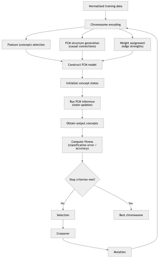
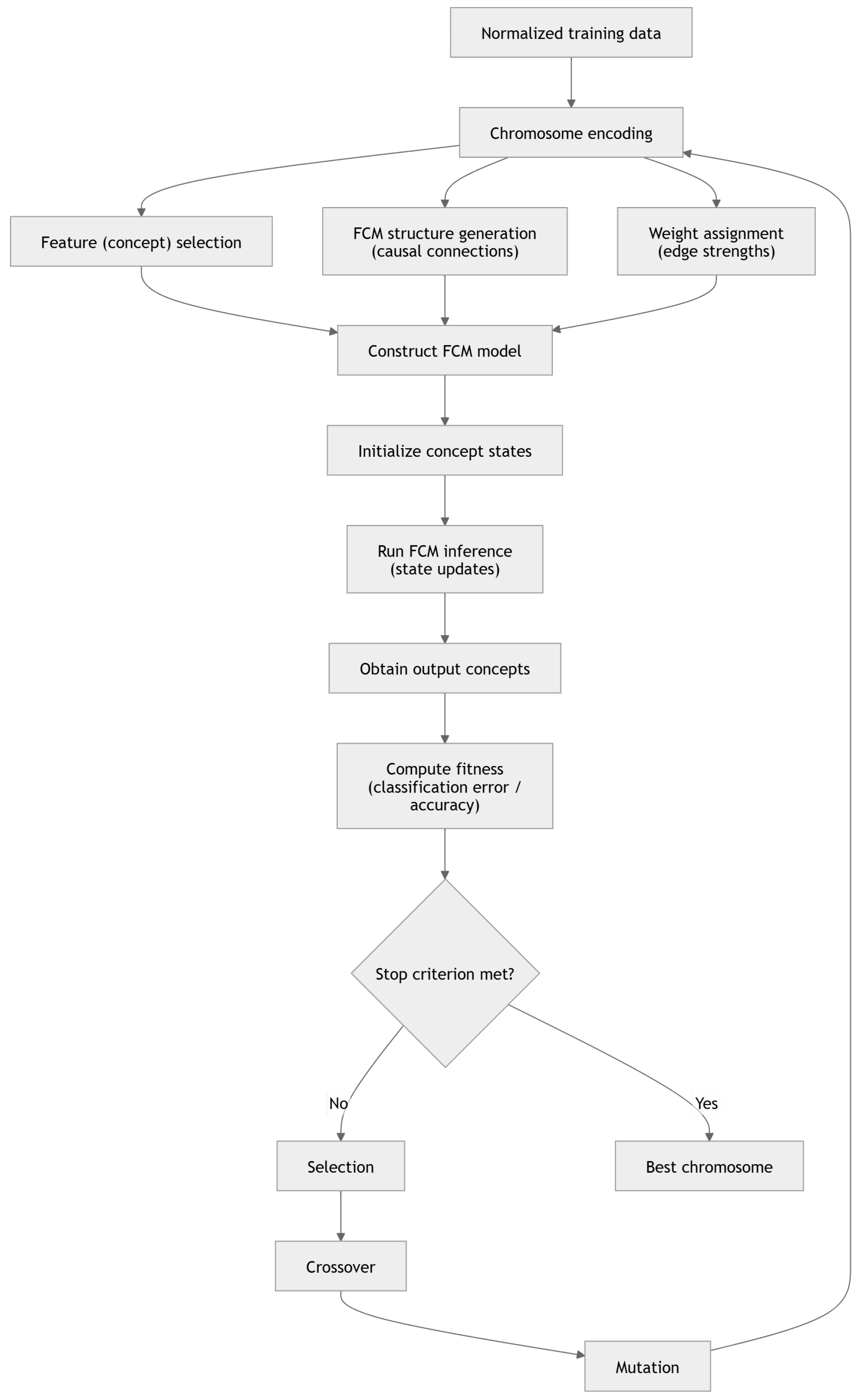
  Genetic Algorithm: The algorithm (specifically designed for FCMs) was analyzed in [49,50]. The general idea is shown in Figure 9.

Figure 9. Flowchart of the genetic algorithm for training the Fuzzy Cognitive Map. The training consists of operations on normalized data: chromosome encoding, feature selection, structure generation (causal connections), and weight assignment, followed by model construction, state initialization, inference, and fitness evaluation. If the stop criterion is not met, genetic operators (selection, crossover, and mutation) are applied until the best chromosome is found.

2.2.2. Multimodal Classification

As mentioned above, the project involved different types of data, each of which can provide useful information on its own. However, many studies have shown that fusing information from different data sources can yield a more accurate classifier. In our research, we selected the data types with the highest MCC values and used them as inputs to a multimodal classifier. Since selecting the appropriate classifier is essential, we tested the following:

• Classical/Reference Approaches: Max-class, averaging, majority voting, XGBoost, and a simple perceptron;
• FCM-Based Approaches:

  –

  Two-stage FCM;

  –

  Multimodal FCM.

Each classifier receives either (i) classification predictions from the data-type-specific FCMs (for the classical approaches and the 2-stage FCM) or (ii) features from each data source (for the multimodal FCM).

Classical/Reference Approaches:

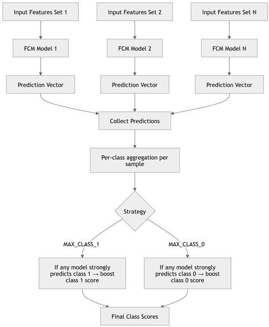
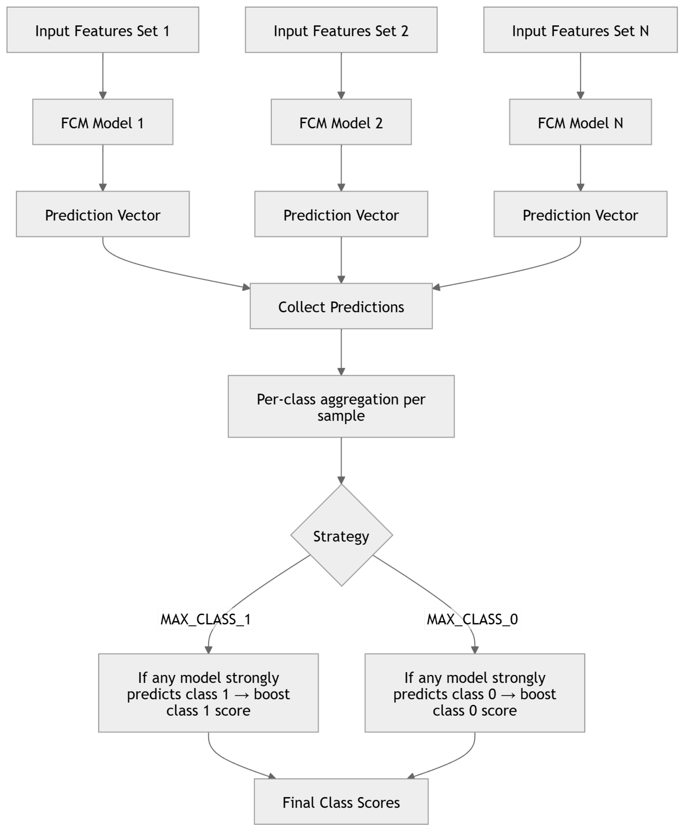
Maximization of one class works as follows: if the chosen class is predicted by any of the data-type-specific FCM classifiers, it is selected as the final classification result, as shown in Figure 10.

Figure 10. MAX_CLASS_1/MAX_CLASS_0 classifier overview. The diagram shows the parallel processing of different feature sets by FCMs, collection of predictions, per-class aggregation, and the final scoring strategy.

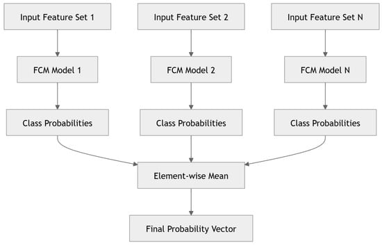
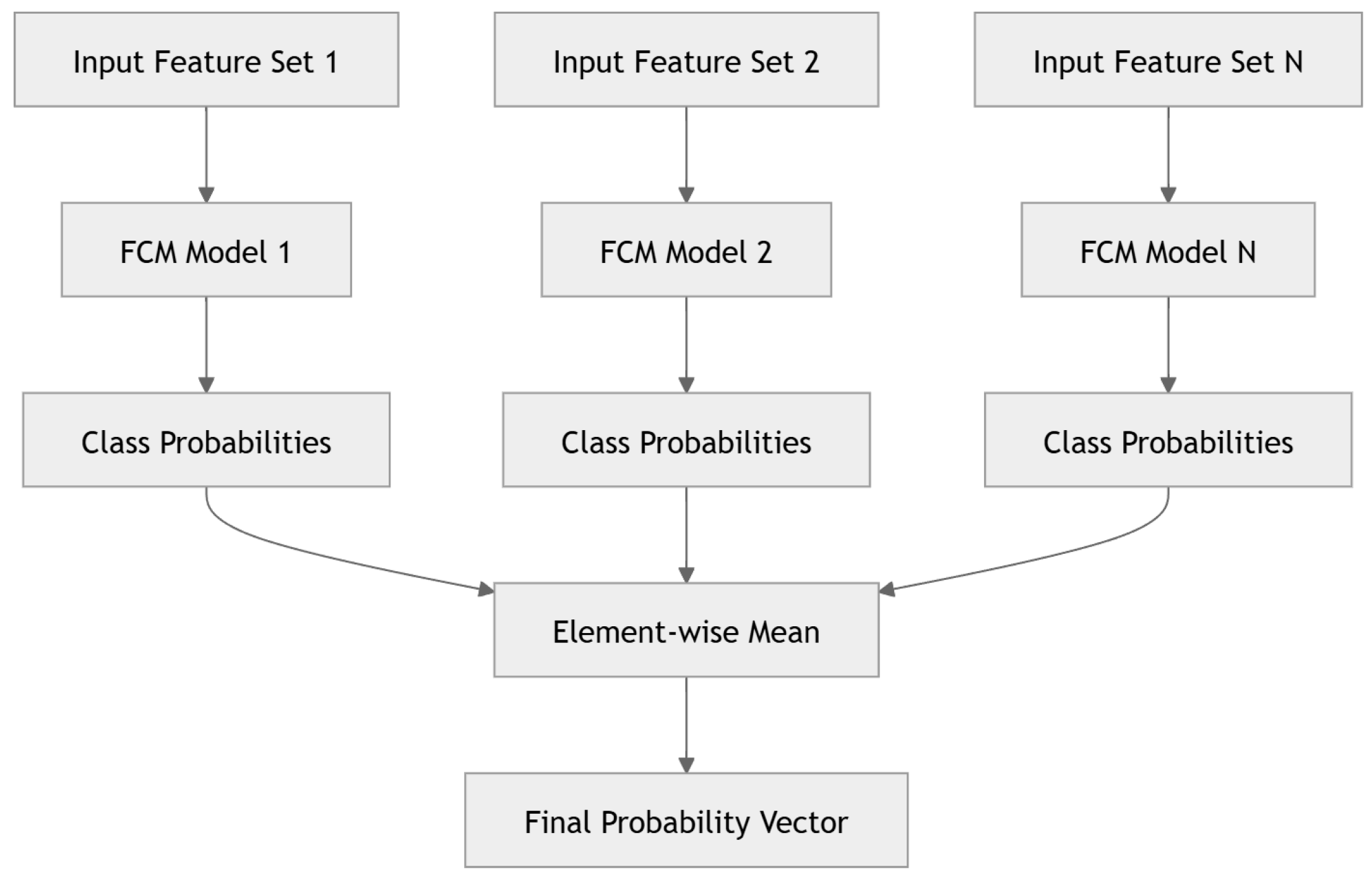
The average classifier combines all results from the data-type-specific FCM classifiers by computing their mean. This approach aggregates the decisions of multiple FCM models across multiple data sources. An overview is shown in Figure 11.

Figure 11. Average classifier overview, which uses the mean of predictions from separate FCM models as the probability estimate.

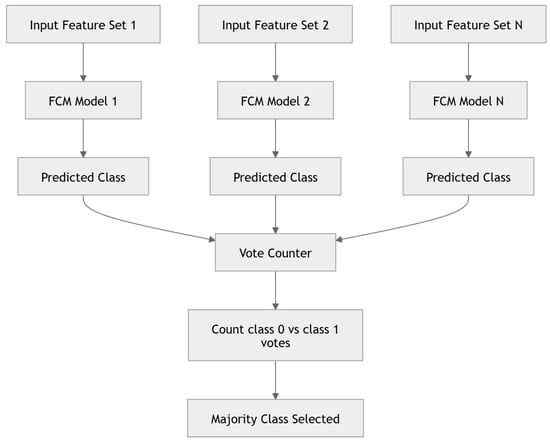
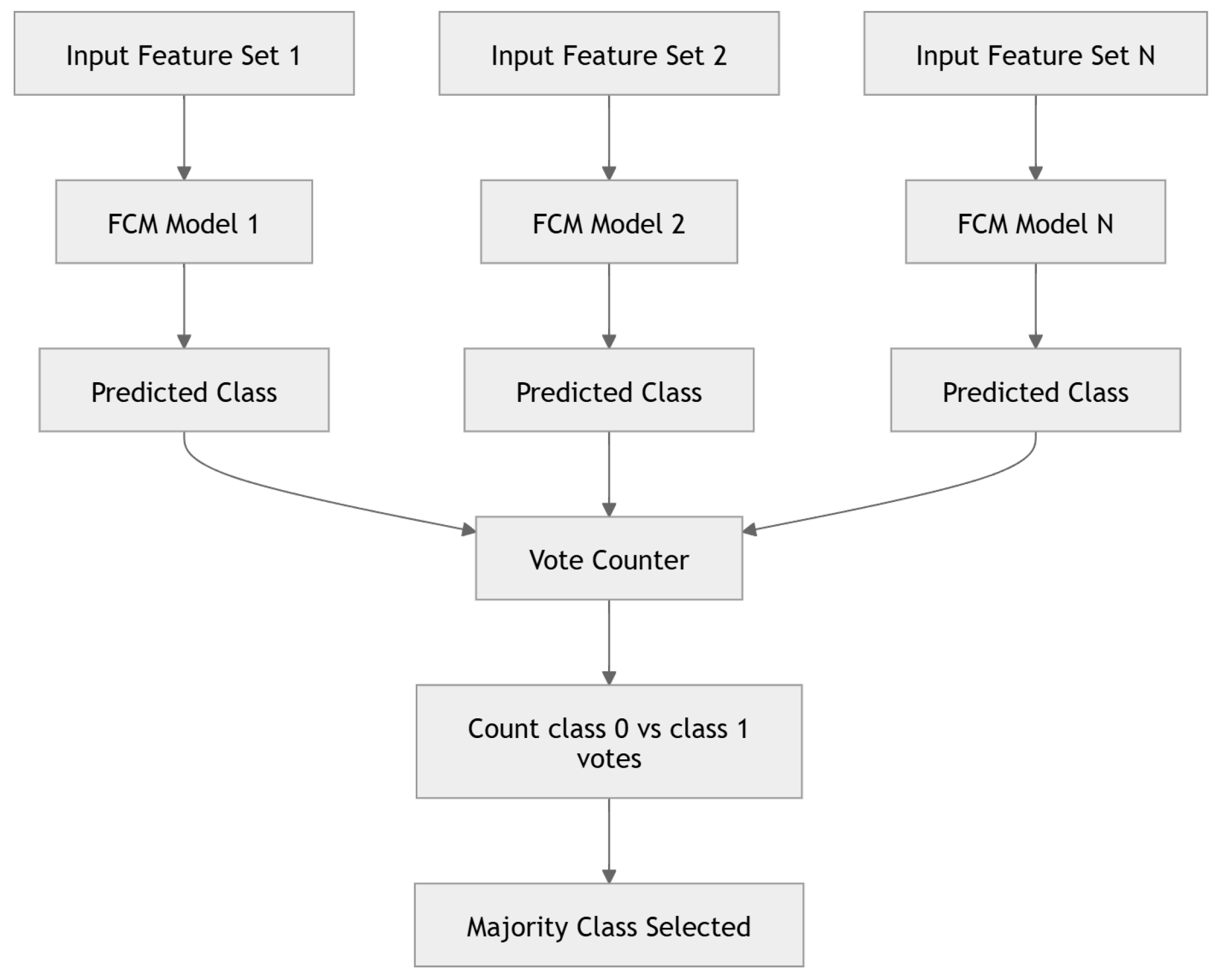
In majority voting, we count how many times each class is predicted by the data-type-specific FCM classifiers and choose the final class based on the majority of votes. If there is a tie, the “Porosity” class is chosen (Figure 12).

Figure 12. Majority voting classifier overview. The classifier counts predictions made by separate FCM models and then applies majority voting to produce the final classification.

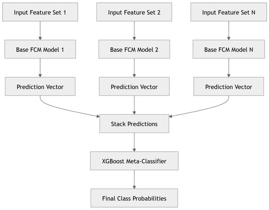
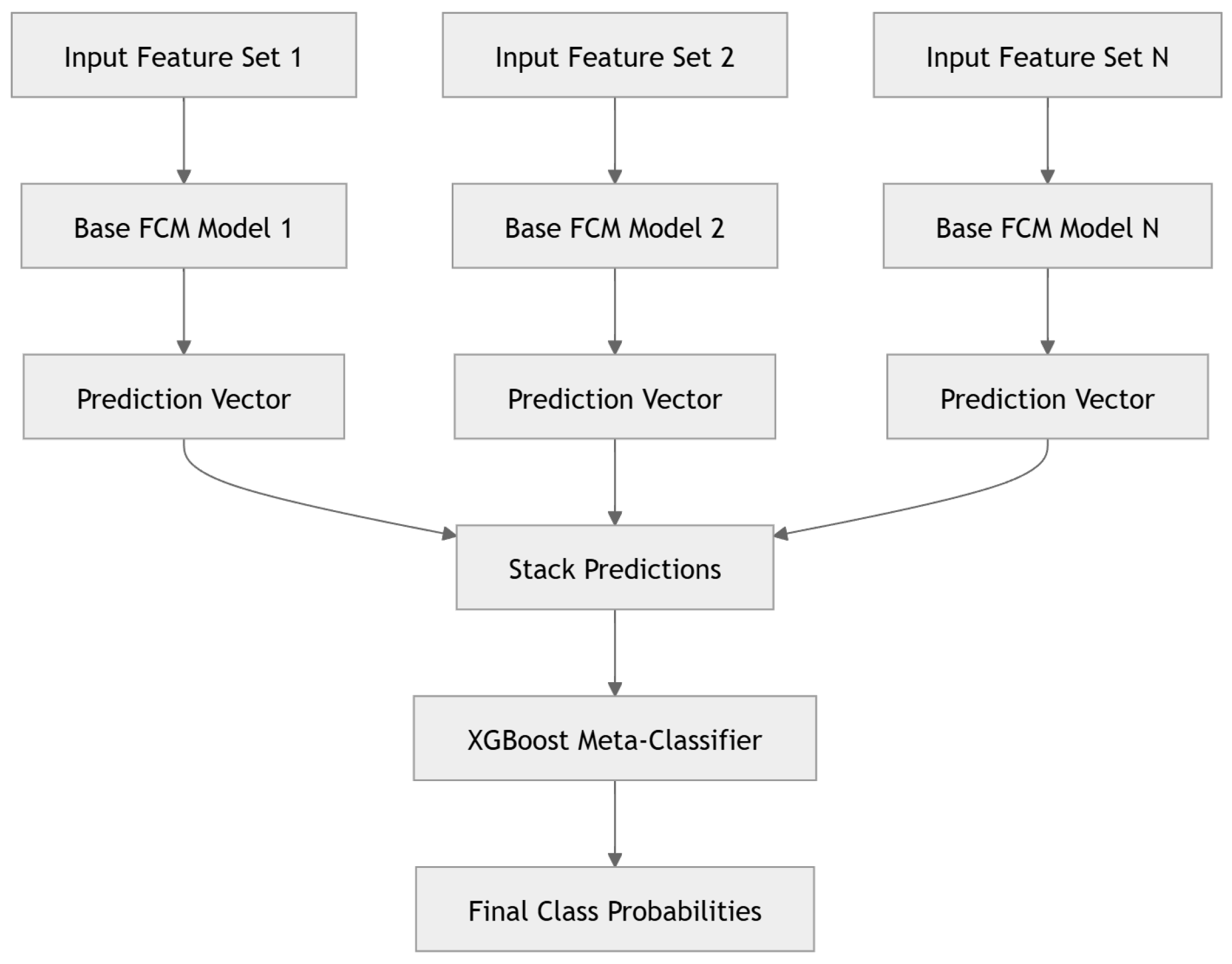
The XGBoost approach uses an XGBoost classifier to produce the final classification from the vector of predictions produced by the data-type-specific FCMs, as shown in Figure 13.

Figure 13. XGBoost-based classifier overview. The classifier stacks all predictions into one vector, which is then processed by the XGBoost classifier to produce the final classification.

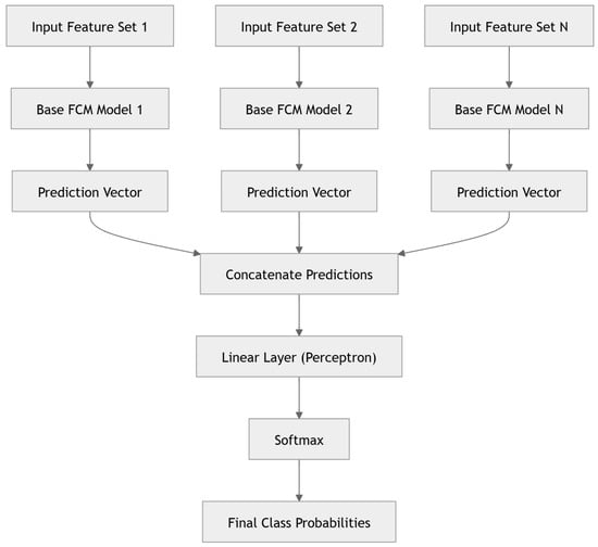
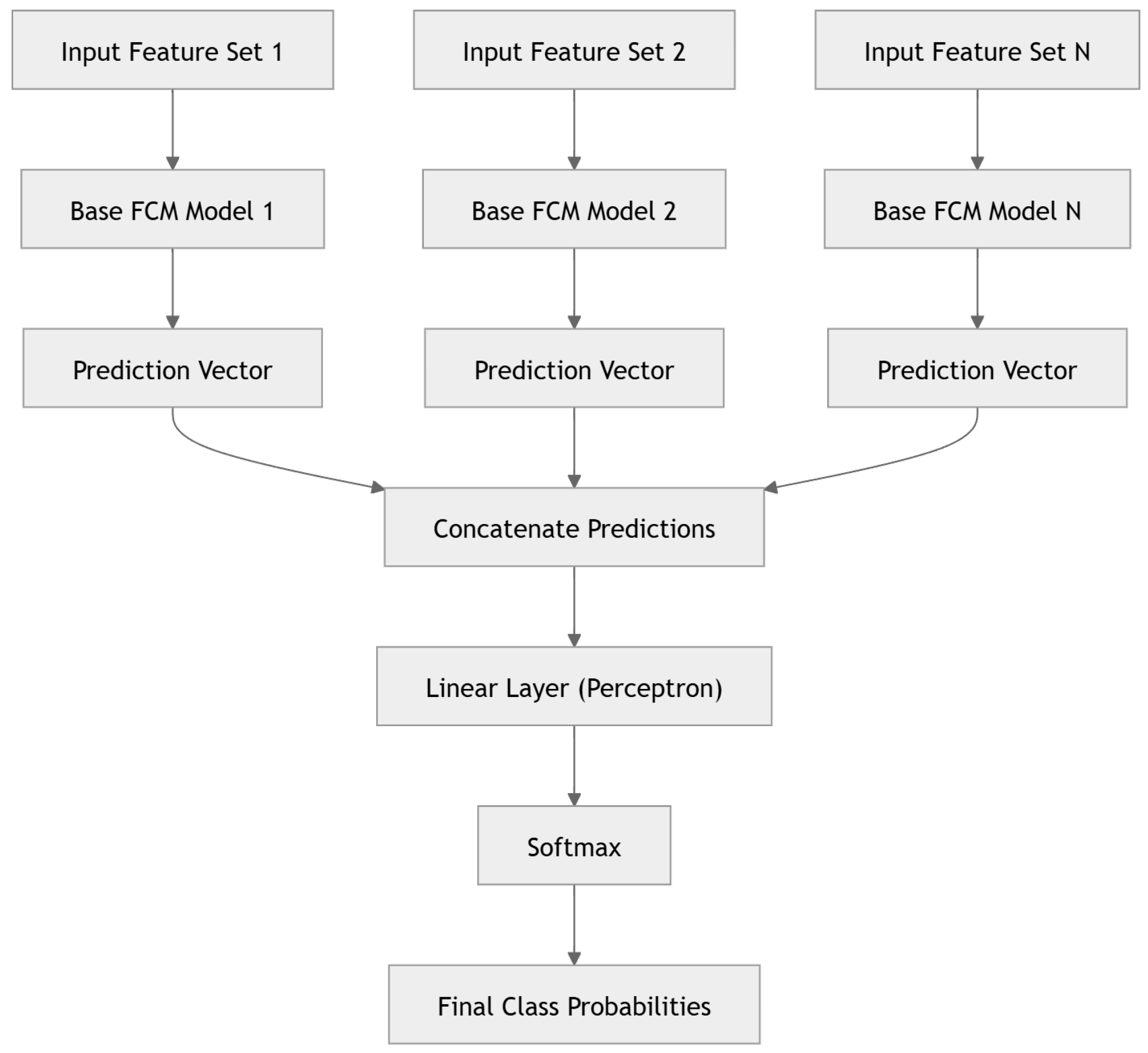
The last reference classifier is a perceptron with a simple linear fully connected layer and a two-dimensional output. As input features, we use the outputs from the separate FCMs. The overview of the classifier is shown in Figure 14.

Figure 14. Perceptron classifier overview. The classifier stacks all predictions into one vector, which is then fed into a linear layer connected to the final softmax output, providing the final classification.

Overview of FCM-Based 2-Step and Multimodal FCM Classifiers:

The 2-step FCM classifier, similarly to the classical/reference approaches, uses the predictions from the separate FCMs as input features. The feature vector is constructed by concatenation and is then processed by a new map, providing the final classification (Figure 15).

Figure 15. Two-step FCM classifier overview. Similarly to XGBoost or the perceptron, it stacks all predictions made by the separate FCM models into one feature vector, which is then classified using an additional FCM.

The multimodal FCM classifier uses features extracted directly from the data sources without intermediate classifiers (e.g., without separate FCMs). For this approach, we considered two variants of inter-source concept interactions, described in the previous subsection and shown in Figure 8. This enables analysis of (i) whether and how different features influence the final classification and (ii) whether concepts can boost each other during inference.

3. Results

To test the proposed approaches, we implemented prototype applications in Python 3.10 that incorporated all components and evaluation ideas described in the previous section. The experiments were conducted on a dataset containing header, time-series, and thermal image data from a real production environment.

The dataset was collected between 2023 and 2025 and contains a total of 383 parts with all three modalities: 383 rows of header data, 383 time-series files, and 766 thermal images (383 before and 383 after spraying). The samples were collected from four different machines and at least four different molds.

Overall, 200 parts were classified as good (OK) and 183 as containing porosity. Training and test sets were created using a random split with the following sizes:

• Training Set: 305 parts (OK: 160, Porosity: 145);
• Test Set: 78 parts (OK: 40, Porosity: 38).

A random split was selected because information about batch membership and production runs was not available in the dataset. For ground truth, all produced parts were examined and labeled by the casting experts. The class labels used in this study correspond to the operational quality assessment provided by the industrial partner. Due to the confidentiality requirements, we are not allowed to disclose all of the details of the inspection and quality assessment. Additionally, the labels should be understood as the operational quality labels, rather than as a direct and exhaustive measurement of the internal porosity and its type, size, or other characteristics.

In industrial HPDC practice, assessment of the parts can be performed using different inspection methods, like visual inspection, X-ray or computed tomography (CT) for in-depth examination, and leak testing [51].

To reduce the risk of data leakage, we split samples from different machines, time periods, runs, and molds into the training and test sets. All splits were created before any model training or selection, and no information from the test set was used during these processes. The test set was used exclusively for final evaluation and was not used for model fine-tuning or parameter selection.

In addition to the main training and test split, we created five random splits for 5-fold cross-validation. For splits 1–3, 306 samples were used for training and 77 for validation; for splits 4 and 5, 307 samples were used for training and 76 for validation. The proportions of classes were kept consistent across folds and sets, with the same number of OK classes and only minor variations in the number of Porosity samples. The summary of the distribution is shown in Table 2. The dataset overview is shown in Table 3.

Table 2. Distribution of OK and Porosity classes across the five-fold cross validation dataset, for the training and validation sets.

	Training Set			Validation Set
Fold	Total	Class OK	Class Porosity	Total	Class OK	Class Porosity
1	306	160	146	77	40	37
2	306	160	146	77	40	37
3	306	160	146	77	40	37
4	307	160	147	76	40	36
5	307	160	147	76	40	36

Table 3. Characteristics of the dataset used in the experiments.

Characteristic	Information
Collection period	2023–2025
Total number of parts	383
Data modalities	Header/process data: 383 rows; time-series data: 383 files; thermal images: 766 images (383 before and 383 after spraying)
Machines	4 different machines
Molds	At least 4 different molds
Class distribution	200 OK parts; 183 parts containing porosity
Ground truth	Leakage tests performed on all produced parts, with final labels assigned by process specialists based on expert knowledge
Random hold-out split
Training set	305 parts (160 OK, 145 Porosity)
Test set	78 parts (40 OK, 38 Porosity)
Split procedure	Random split performed before model training and model selection. Samples originate from different machines, times, production runs, and molds. The test set was used exclusively for final evaluation.

During evaluation, all steps required to prepare the data for model training were performed using only the training data. In particular, normalization parameters, PCA transformations, and the feature-selection procedure were computed exclusively on the training set and then applied unchanged to the test set during final evaluation. Similarly, DTW reference sequences were determined only from the training data and then used to compute DTW-based features for the test set. The test set was not used at any stage of fitting, selection, or determining any model components.

We evaluated algorithm performance using the Matthews Correlation Coefficient (MCC) [52], which is one of the most reliable metrics [53] and is defined as follows:

$$\mathrm{MCC}={\displaystyle \frac{TP\times TN-FP\times FN}{\sqrt{(TP+FP)(TP+FN)(TN+FP)(TN+FN)}}}$$

(12)

where $TP$ is true positives, $TN$ true negatives, $FP$ false positives, and $FN$ false negatives.

The first experiments were designed to address the following research questions:

• How does feature dimensionality reduction (PCA) influence the results?
• How do different weight-selection algorithms influence the results?
• How do different data sources influence the results?

The aggregated results are shown in Table 4 and Table 5. We group the tests into centroid-based algorithms (Table 4) and classical (non-centroid) algorithms (Table 5) to evaluate which approach provides better performance.

Table 4. A comparison of MCC metrics for different algorithms based on centroids, across various data types, preprocessing versions, and PCA settings.

Data	Version	PCA	Gradient Descent	Particle Swarm	Tziolas et al. [33]	Hebbian Learning	Differential Hebbian	Simulated Annealing	Pseudo- Inverse
header	normalized	-	0.4977	0.4583	0.4670	0.5192	0.5193	0.4779	0.4665
header	normalized	0.9	0.5161	0.5354	0.4385	0.4036	0.4648	0.4955	0.4398
header	normalized	0.99	0.4641	0.4818	0.4743	0.4925	0.4722	0.4817	0.5233
images	our extractor	-	0.3211	0.5030	0.3142	0.2815	0.3854	0.2928	0.2815
images	our extractor	0.9	0.6301	0.6301	0.6301	0.6301	0.6301	0.6301	0.6301
images	our extractor	0.99	0.4352	0.6539	0.4318	0.5261	0.4073	0.4456	0.4412
images	DINOv2	-	0.4092	0.6376	0.5193	0.4623	0.5185	0.5953	0.5182
images	DINOv2	0.9	0.6235	0.6677	0.6576	0.6052	0.5897	0.6423	0.5842
images	DINOv2	0.99	0.5338	0.5953	0.5966	0.5605	0.5966	0.5896	0.4903
images	DINOv2 Siamese	-	0.5915	0.7080	0.5992	0.5811	0.6631	0.6335	0.6774
images	DINOv2 Siamese	0.9	0.7504	0.7099	0.6680	0.6441	0.6864	0.6910	0.6315
images	DINOv2 Siamese	0.99	0.6315	0.6374	0.6436	0.6315	0.6251	0.6369	0.6446
profiles	statistical	-	0.3758	0.3070	0.4010	0.4002	0.3823	0.3894	0.3929
profiles	statistical	0.9	0.3803	0.3649	0.3723	0.3938	0.3680	0.4217	0.3336
profiles	statistical	0.99	0.3735	0.3002	0.3680	0.3432	0.3685	0.3688	0.3339
profiles	DTW	-	0.3201	0.3039	0.3201	0.3201	0.3201	0.3201	0.3201
profiles	DTW	0.9	0	0	0	0	0	0	0
profiles	DTW	0.99	0.1983	0.1951	0.1983	0.1983	0.1951	0.1951	0.1983

Table 5. A comparison of MCC metrics for different algorithms that are not based on centroids, across data types, preprocessing versions, and PCA settings.

Data	Version	PCA	Gradient Descent	Genetic Algorithm
header	normalized	-	0.2623	0.4047
header	normalized	0.9	0.5895	0.5663
header	normalized	0.99	0.5671	0.5422
images	our extractor	-	0.6072	0.0745
images	our extractor	0.9	0.5475	0.5712
images	our extractor	0.99	0.6072	0.6966
images	DINOv2	-	0.6284	−0.0945
images	DINOv2	0.9	0.2403	0.6178
images	DINOv2	0.99	0.1169	0.1307
images	DINOv2 Siamese	-	0.9233	−0.0526
images	DINOv2 Siamese	0.9	0.8984	0.6720
images	DINOv2 Siamese	0.99	0.7390	0.1748
profiles	statistical	-	0.5428	0.2089
profiles	statistical	0.9	0.2296	0.1664
profiles	statistical	0.99	0.5152	0.3793
profiles	DTW	-	−0.0074	0.0413
profiles	DTW	0.9	0.0000	0.0918
profiles	DTW	0.99	0.0000	0.2282

Overall, the highest performance was obtained using thermal images and header data, while the lowest was obtained using time-series data. Thermal images capture the thermal state after part removal and just before filling the mold with molten metal, which can be beneficial for defect detection in HPDC because many defect mechanisms are directly linked to temperature. Header data contain process parameters and sensor readouts as a single feature vector per shot, which is easier to analyze than full time series. Although time-series performance was lowest in our experiments, it may still contain meaningful information; in future work, we will investigate whether improved processing or time-series-specific model architectures can improve performance.

Another insight from the experiments is that, on average, the highest MCC values were obtained when applying PCA and retaining 90% of the components. The only exception was DTW features extracted from profiles, for which the unreduced version achieved the highest values. For each data type, the following algorithms achieved the highest MCC values:

• Header (normalized): Classical gradient descent (0.5895), followed by the genetic algorithm (0.5663);
• Images (our feature extractor): Genetic algorithm (0.6966), followed by centroids-based particle swarm optimization (0.6539);
• Images (DINOv2 features): Centroids-based particle swarm optimization (0.6677), followed by classical gradient descent (0.6284);
• Images (DINOv2 Siamese features): Classical gradient descent (0.9233), followed by centroids-based gradient descent (0.7504);
• Profiles (statistical features): Classical gradient descent (0.5428), followed by centroids-based simulated annealing (0.4217);
• Profiles (DTW features): Centroids-based algorithms achieved similar and higher values (max 0.3201) than classical ones (max 0.2282).

These results indicate that there is no universal algorithm for all data types and that the optimal configuration should be selected separately for each modality. Additionally, performance depends strongly on the selected feature-reduction variant.

The next set of experiments focused on classification using fused information from different data sources. The results are presented in Table 6. The following inputs were used for each model variant:

Table 6. Results for the multi-classifier test set, including the FCM ablation variants.

Model Variant	Method	MCC	Number of Feature Sets	Inter-Source Weights Influence
M1	PERCEPTRON	0.6921	3	N/A
M1.5	PERCEPTRON	0.3934	3	N/A
M2	XGBoost	0.7961	3	N/A
M2.5	XGBoost	0.8460	3	N/A
M3	LIGHTGBM	0.8474	3	N/A
M3.5	LIGHTGBM	0.8974	3	N/A
M4	MAJORITY VOTE	0.5947	3	N/A
M5	MAX CLASS 0	0.7467	3	N/A
M6	MAX CLASS 1	0.7533	3	N/A
M7	AVERAGE	0.6921	3	N/A
M8	2-stage FCM (centroids),	0.8208	3	Separate sets
M9	2-stage FCM (centroids),	0.8208	3	Merged sets
M10	Multimodal FCM (no centroids) GA	0.7182	3	Merged input
M11	Multimodal FCM (no centroids)	0.4113	3	Separate sets
M12	Multimodal FCM (no centroids)	0.4113	3	Merged input
M13	2-stage FCM (no centroids)	0.7514	3	Merged input
M14	2-stage FCM (no centroids)	0.7514	3	Separate sets
M15	2-stage FCM (no centroids)	0.8225	2	Separate sets
M16	2-stage FCM (no centroids)	0.8225	2	Merged input
M17	Multimodal FCM (no centroids)	0.8793	2	Separate sets
M18	Multimodal FCM (no centroids)	0.7947	2	Merged input
M19	2-stage FCM (no centroids)	0.8208	2	Separate sets
M20	2-stage FCM (no centroids)	0.8208	2	Merged input
M21	Multimodal FCM (no centroids)	0.8741	2	Separate sets
M22	Multimodal FCM (no centroids)	0.8741	2	Merged input

• M1–M10, except M1.5, M2.5, and M3.5: Outputs of three FCMs: (i) particle swarm optimization, normalized header data with 0.9 PCA; (ii) centroids-based gradient descent, DINOv2 Siamese features with 0.9 PCA; (iii) centroids-based gradient descent, DTW profile features without PCA.
• M1.5, M2.5, and M3.5: Normalized header data with 0.9 PCA, DINOv2 Siamese features with 0.9 PCA, and DTW profile features without PCA.
• M13–M14: Outputs of three FCMs: (i) particle swarm optimization, normalized header data with 0.9 PCA; (ii) classical gradient descent, DINOv2 Siamese features without PCA; (iii) centroids-based gradient descent, DTW profile features without PCA.
• M11–M12: Raw feature sets: normalized header data with 0.9 PCA, DINOv2 Siamese features without PCA, and DTW profile features without PCA.
• M15–M16: Outputs of two FCMs: (i) particle swarm optimization, normalized header data with 0.9 PCA; (ii) classical gradient descent, DINOv2 Siamese features without PCA.
• M17–M18: Raw feature sets: normalized header data with 0.9 PCA and DINOv2 Siamese features without PCA.
• M19–M20: Outputs of two FCMs: (i) particle swarm optimization, normalized header data with 0.9 PCA; (ii) classical gradient descent, DINOv2 Siamese features with 0.9 PCA.
• M21–M22: Raw feature sets: normalized header data with 0.9 PCA and DINOv2 Siamese features with 0.9 PCA.

For the non-FCM approaches (M1–M7), both LightGBM classifiers (M3 and M3.5) and M2.5 achieved the highest MCC value (0.8474 for M3 and 0.8974 for M3.5). For the two-stage FCMs (M8 and M9), the highest MCC value was slightly lower. Notably, both LightGBM and XGBoost models achieved an MCC of 1.0 on the training set, compared to 0.8826 for the two-stage FCMs; we investigate this further using cross-validation. In addition, we evaluated a multimodal FCM (M10) that uses a genetic algorithm for concept and weight selection. Its MCC was lower than that of many other approaches; however, map complexity was also substantially lower, which may be beneficial in some applications.

We also performed experiments using three input data types with different thermal-image training variants (M11–M14). In these settings, performance was lower than in the previous experiments for both two-stage and multimodal FCMs.

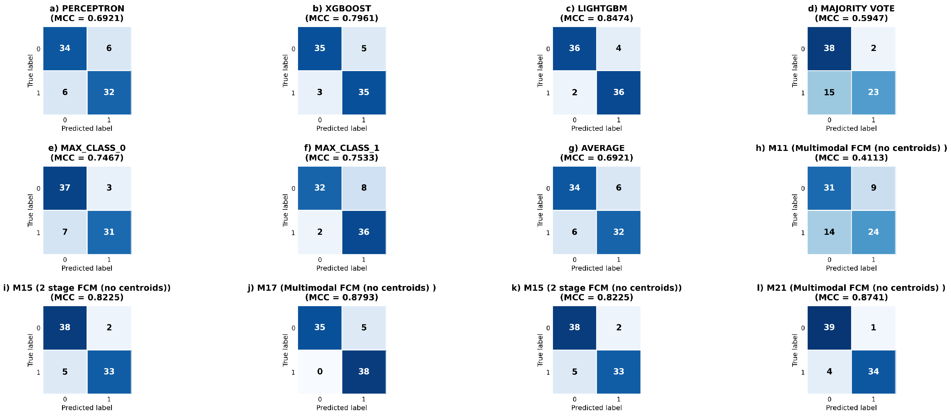
Finally, we performed experiments with reduced inputs using only header and thermal data (M15–M22). In this case, the multimodal FCM without centroids achieved the highest MCC value (0.8793 for M17). Because M17 has high complexity (all thermal image features were used), we also tested PCA-reduced inputs. In this setting, the MCC for the multimodal FCMs (M21 and M22) was only slightly lower (0.8741), while model complexity was significantly reduced.

Overall, the multimodal fusion results do not provide strong evidence that fusion improves classification performance. The best single-modality FCM model (DINOv2 Siamese trained with classical gradient descent without centroids) achieved an MCC of 0.9233, while the best multimodal FCM models (M17 and M21) achieved MCC values of 0.8793 and 0.8741, respectively. Although the difference is not large, it favors the data-source-specific model. Moreover, several two-stage and multimodal FCM variants achieved substantially lower performance, indicating that naively adding more modalities does not necessarily improve results. The baseline models LightGBM and HP-GAN reached MCC values of 0.8474 and 0.6280, respectively, showing that FCM-based approaches can achieve higher performance.

A possible explanation for the slightly higher performance of the DINOv2 Siamese model is that thermal images contain highly discriminative information related to physical effects leading to porosity. The additional header data may be partially redundant or may require further processing to extract complementary information. Moreover, time-series data did not improve the results and did not achieve usable performance even when used alone, suggesting either that the signal is not informative for this task or that different preprocessing and/or model architectures are required. Finally, our results indicate that the fusion strategy itself has a substantial impact on the final performance.

Finally, we evaluated the HP-GAN algorithm using the same input data (header and thermal images); the results are shown in Table 7. Our HP-GAN implementation and training/tuning procedure were based on publicly available information, without code provided by the authors. Therefore, the HP-GAN results should be treated as an adapted implementation, since the original code was not available.

Table 7. The test results for HP-GAN models on different types of data.

Data	Version	Algorithm	MCC
Header	Normalized	HP-GAN header only	0.4850
Images	Raw images	HP-GAN images only	0.5470
Header and images	Normalized + raw images	Original HP-GAN	0.6280

The comparison of HP-GAN with the FCM and LightGBM models was performed under identical conditions, using the same dataset and data splits. Consequently, the data preprocessing and evaluation protocol were also identical.

For each HP-GAN variant, the best data-type-specific FCM models outperformed HP-GAN. Additionally, for multimodal classification, most non-FCM approaches achieved higher MCC values than HP-GAN.

To further evaluate the proposed models and verify that the findings are consistent with the initial hold-out test set, we performed 5-fold cross-validation using all 383 available samples.

The results for the selected models are shown in Table 8 and Table 9. For most data-type-specific FCMs (Table 8), performance was similar to the initial test-set results, suggesting that the hold-out split is representative. For the multimodal models (Table 9), performance was generally slightly lower, with a notable decrease for M12. In contrast to the other models, HP-GAN achieved a slightly higher MCC than some multimodal variants; however, its performance remained substantially lower than that of the best FCM models.

Table 8. Five-fold cross-validation results for selected FCM models and feature types. Values are reported as the mean ± standard deviation. Algorithms: PSO—particle swarm optimization, GD—gradient descent, SA—simulated annealing, CD—centroids-based, GA—genetic algorithm. Note: These results were obtained using the original cross-validation protocol, with PCA fitted on the original training set prior to the five-fold partitioning.

Data	Version	PCA	Centroids	Algorithm	Performance Metric for the Validation Set
					MCC	Balanced Accuracy	F1 Score OK	F1 Score Porosity	Recall OK	Recall Porosity
header	normalized	0.9	yes	PSO	$0.4939\pm 0.1658$	$0.7362\pm 0.0871$	$0.7129\pm 0.1152$	$0.7398\pm 0.1013$	$0.6600\pm 0.1701$	$0.8125\pm 0.1778$
header	normalized	0.9	yes	GD	$0.3797\pm 0.1683$	$0.6835\pm 0.0854$	$0.7330\pm 0.0641$	$0.6264\pm 0.1155$	$0.8100\pm 0.0518$	$0.5569\pm 0.1337$
header	normalized	0.9	no	GD	$0.5226\pm 0.0909$	$0.7595\pm 0.0446$	$0.7511\pm 0.0506$	$0.7618\pm 0.0427$	$0.7050\pm 0.0716$	$0.8140\pm 0.0626$
images	our extractor	0.9	yes	PSO	$0.6116\pm 0.0334$	$0.8007\pm 0.0178$	$0.8245\pm 0.0144$	$0.7786\pm 0.0225$	$0.8800\pm 0.0112$	$0.7215\pm 0.0336$
images	our extractor	0.9	yes	GD	$0.6116\pm 0.0334$	$0.8007\pm 0.0178$	$0.8245\pm 0.0144$	$0.7786\pm 0.0225$	$0.8800\pm 0.0112$	$0.7215\pm 0.0336$
images	our extractor	0.9	no	GD	$0.6116\pm 0.0334$	$0.8007\pm 0.0178$	$0.8245\pm 0.0144$	$0.7786\pm 0.0225$	$0.8800\pm 0.0112$	$0.7215\pm 0.0336$
images	our extractor	0.99	no	GA	$0.6660\pm 0.0460$	$0.8282\pm 0.0150$	$0.7960\pm 0.0271$	$0.8466\pm 0.0261$	$0.7076\pm 0.0687$	$0.9488\pm 0.0460$
images	DINOv2	0.9	yes	PSO	$0.6771\pm 0.0747$	$0.8380\pm 0.0380$	$0.8457\pm 0.0315$	$0.8297\pm 0.0434$	$0.8450\pm 0.0209$	$0.8309\pm 0.0717$
images	DINOv2	0.9	yes	GD	$0.5791\pm 0.0743$	$0.7780\pm 0.0415$	$0.8142\pm 0.0299$	$0.7398\pm 0.0594$	$0.9050\pm 0.0209$	$0.6511\pm 0.0832$
images	DINOv2	0.9	no	GD	$0.2378\pm 0.1061$	$0.5916\pm 0.0430$	$0.7070\pm 0.0293$	$0.3965\pm 0.0818$	$0.9100\pm 0.0335$	$0.2733\pm 0.0642$
images	DINOv2-Siamese	0.9	yes	PSO	$0.7338\pm 0.0438$	$0.8617\pm 0.0182$	$0.8758\pm 0.0200$	$0.8499\pm 0.0196$	$0.9200\pm 0.0542$	$0.8033\pm 0.0444$
images	DINOv2-Siamese	0.9	yes	GD	$0.6982\pm 0.0632$	$0.8477\pm 0.0331$	$0.8571\pm 0.0247$	$0.8383\pm 0.0403$	$0.8650\pm 0.0224$	$0.8303\pm 0.0758$
images	DINOv2-Siamese	-	no	GD	$0.8113\pm 0.0847$	$0.9018\pm 0.0466$	$0.9101\pm 0.0385$	$0.8941\pm 0.0537$	$0.9250\pm 0.0468$	$0.8787\pm 0.1072$
images	DINOv2-Siamese	0.9	no	GD	$0.8399\pm 0.0432$	$0.9172\pm 0.0218$	$0.9249\pm 0.0204$	$0.9120\pm 0.0235$	$0.9550\pm 0.0326$	$0.8794\pm 0.0329$
profiles	statistical	0.9	yes	SA	$0.3468\pm 0.1214$	$0.6582\pm 0.0529$	$0.7188\pm 0.0665$	$0.5825\pm 0.0441$	$0.8300\pm 0.1204$	$0.4863\pm 0.0515$
profiles	statistical	0.9	yes	GD	$0.3468\pm 0.1214$	$0.6582\pm 0.0529$	$0.7188\pm 0.0665$	$0.5825\pm 0.0441$	$0.8300\pm 0.1204$	$0.4863\pm 0.0515$
profiles	statistical	0.9	no	GD	$0.2528\pm 0.1549$	$0.6260\pm 0.0772$	$0.6373\pm 0.0890$	$0.6134\pm 0.0709$	$0.6350\pm 0.1098$	$0.6170\pm 0.0649$
profiles	DTW	-	yes	PSO	$0.2703\pm 0.1005$	$0.6142\pm 0.0535$	$0.7005\pm 0.0291$	$0.4735\pm 0.1310$	$0.8450\pm 0.1165$	$0.3835\pm 0.1954$
profiles	DTW	-	yes	GD	$0.3044\pm 0.0637$	$0.5936\pm 0.0300$	$0.7258\pm 0.0152$	$0.3281\pm 0.0858$	$0.9850\pm 0.0137$	$0.2023\pm 0.0634$
profiles	DTW	-	no	GD	$0.0519\pm 0.0898$	$0.5107\pm 0.0224$	$0.1157\pm 0.0638$	$0.6422\pm 0.0157$	$0.0650\pm 0.0379$	$0.9565\pm 0.0310$

Table 9. Five-fold cross-validation results for the selected models and the HP-GAN baseline. Values are reported as the mean ± standard deviation. Note: These results were obtained using the original cross-validation protocol, with PCA fitted on the original training set prior to the five-fold partitioning.

Model	Method	Performance Metric
		MCC	Balanced Accuracy	F1 Score OK	F1 Score Porosity	Recall OK	Recall Porosity
M1.5	Perceptron (initial inputs)	$0.1648\pm 0.1566$	$0.5550\pm 0.0683$	$0.4122\pm 0.3775$	$0.4734\pm 0.2554$	$0.5150\pm 0.5011$	$0.5950\pm 0.4548$
M2.5	XGBoost (initial inputs)	$0.8600\pm 0.0536$	$0.9285\pm 0.0278$	$0.9338\pm 0.0250$	$0.9245\pm 0.0304$	$0.9500\pm 0.0306$	$0.9069\pm 0.0467$
M3	LightGBM (FCMs outputs as inputs)	$0.7551\pm 0.0354$	$0.8761\pm 0.0164$	$0.8842\pm 0.0189$	$0.8693\pm 0.0156$	$0.9000\pm 0.0395$	$0.8523\pm 0.0173$
M3.5	LightGBM (initial inputs)	$0.8710\pm 0.0509$	$0.9335\pm 0.0267$	$0.9389\pm 0.0243$	$0.9297\pm 0.0289$	$0.9600\pm 0.0335$	$0.9069\pm 0.0467$
M8	Two-stage FCM (centroids)	$0.8077\pm 0.0254$	$0.9026\pm 0.0124$	$0.9086\pm 0.0113$	$0.8973\pm 0.0139$	$0.9200\pm 0.0326$	$0.8851\pm 0.0357$
M12	Multimodal FCM (no centroids)	$0.1886\pm 0.0724$	$0.5935\pm 0.0353$	$0.5969\pm 0.0362$	$0.5858\pm 0.0457$	$0.5800\pm 0.0647$	$0.6071\pm 0.0834$
M14	Two-stage FCM (no centroids)	$0.7990\pm 0.0482$	$0.8883\pm 0.0270$	$0.9064\pm 0.0206$	$0.8746\pm 0.0333$	$0.9900\pm 0.0137$	$0.7866\pm 0.0464$
M17	Multimodal FCM (no centroids)	$0.5916\pm 0.2442$	$0.7677\pm 0.1433$	$0.6908\pm 0.3163$	$0.7811\pm 0.1099$	$0.6850\pm 0.3843$	$0.8505\pm 0.2077$
M19	Two-stage FCM (no centroids)	$0.8028\pm 0.0248$	$0.8999\pm 0.0125$	$0.9064\pm 0.0107$	$0.8942\pm 0.0145$	$0.9200\pm 0.0326$	$0.8797\pm 0.0412$
M21	Multimodal FCM (no centroids)	$0.8387\pm 0.0439$	$0.9178\pm 0.0215$	$0.9240\pm 0.0209$	$0.9132\pm 0.0227$	$0.9450\pm 0.0326$	$0.8905\pm 0.0205$
	HP-GAN (header and images)	$0.6791\pm 0.0665$	$0.8243\pm 0.0285$	$0.8542\pm 0.0281$	$0.7965\pm 0.0307$	$0.9550\pm 0.0512$	$0.6937\pm 0.0270$

To analyze the train–test gap and further investigate potential overfitting in the LightGBM model, we also evaluated selected models on the training subsets within each cross-validation fold. The results are shown in Table 10. The M3 LightGBM model exhibits a substantially larger train–validation gap than the other models: the MCC increases from $0.7551\pm 0.0354$ on the validation folds to $0.9896\pm 0.0087$ on the corresponding training subsets. A larger gap can also be observed for the LightGBM model with inputs using initial features, not processed by any FCMs—the MCC increases from $0.8710\pm 0.0509$ to $1.0000\pm 0.0000$. A similar situation can be seen for the M2.5 XGBoost model. Additionally, a value of $1.0000$ for all folds and metrics for M2.5 and M3.5 indicates a very high possibility of overfitting. In contrast, for DINOv2 Siamese, M8, and M21, the gap is relatively small, suggesting that these models are less prone to overfitting.

Table 10. Five-fold cross-validation results for the selected models on the training data. Values are reported as the mean ± standard deviation. Note: These results were obtained using the original cross-validation protocol, with PCA fitted on the original training set prior to the five-fold partitioning.

Model	Method	Performance Metric
		MCC	Balanced Accuracy	F1 Score OK	F1 Score Porosity	Recall OK	Recall Porosity
-	DINOv2-Siamese, PCA 0.9, no centroids, GD	$0.8586\pm 0.0152$	$0.9276\pm 0.0069$	$0.9335\pm 0.0070$	$0.9235\pm 0.0073$	$0.9563\pm 0.0188$	$0.8989\pm 0.0148$
M1.5	Perceptron (initial inputs)	$0.3488\pm 0.0566$	$0.6263\pm 0.0505$	$0.7364\pm 0.0152$	$0.4221\pm 0.1518$	$0.9563\pm 0.0532$	$0.2964\pm 0.1531$
M2.5	XGBoost (initial inputs)	$1.0000\pm 0.0000$	$1.0000\pm 0.0000$	$1.0000\pm 0.0000$	$1.0000\pm 0.0000$	$1.0000\pm 0.0000$	$1.0000\pm 0.0000$
M3	LightGBM	$0.9896\pm 0.0087$	$0.9945\pm 0.0046$	$0.9950\pm 0.0041$	$0.9945\pm 0.0046$	$1.0000\pm 0.0000$	$0.9891\pm 0.0092$
M3.5	LightGBM (initial inputs)	$1.0000\pm 0.0000$	$1.0000\pm 0.0000$	$1.0000\pm 0.0000$	$1.0000\pm 0.0000$	$1.0000\pm 0.0000$	$1.0000\pm 0.0000$
M8	Two-stage FCM (centroids)	$0.8065\pm 0.0061$	$0.9026\pm 0.0031$	$0.9086\pm 0.0028$	$0.8975\pm 0.0035$	$0.9200\pm 0.0081$	$0.8852\pm 0.0090$
M21	Multimodal FCM (no centroids)	$0.8490\pm 0.0088$	$0.9231\pm 0.0042$	$0.9291\pm 0.0042$	$0.9188\pm 0.0045$	$0.9500\pm 0.0117$	$0.8962\pm 0.0103$

In addition, we used cross-validation to verify whether the same trend holds when comparing DINOv2 Siamese and multimodal FCM models. The results, consistent with the initial hold-out test set, indicate that adding more modalities does not substantially improve performance.

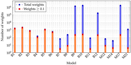
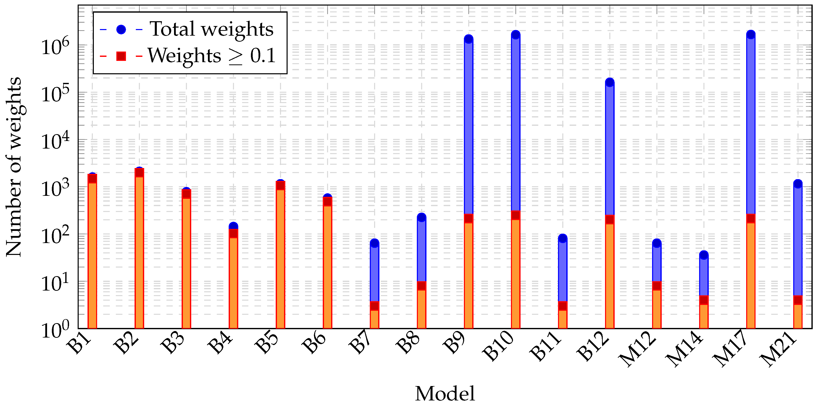
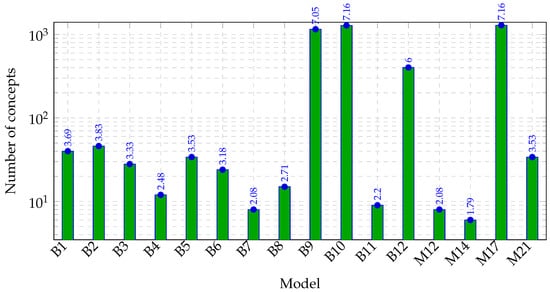
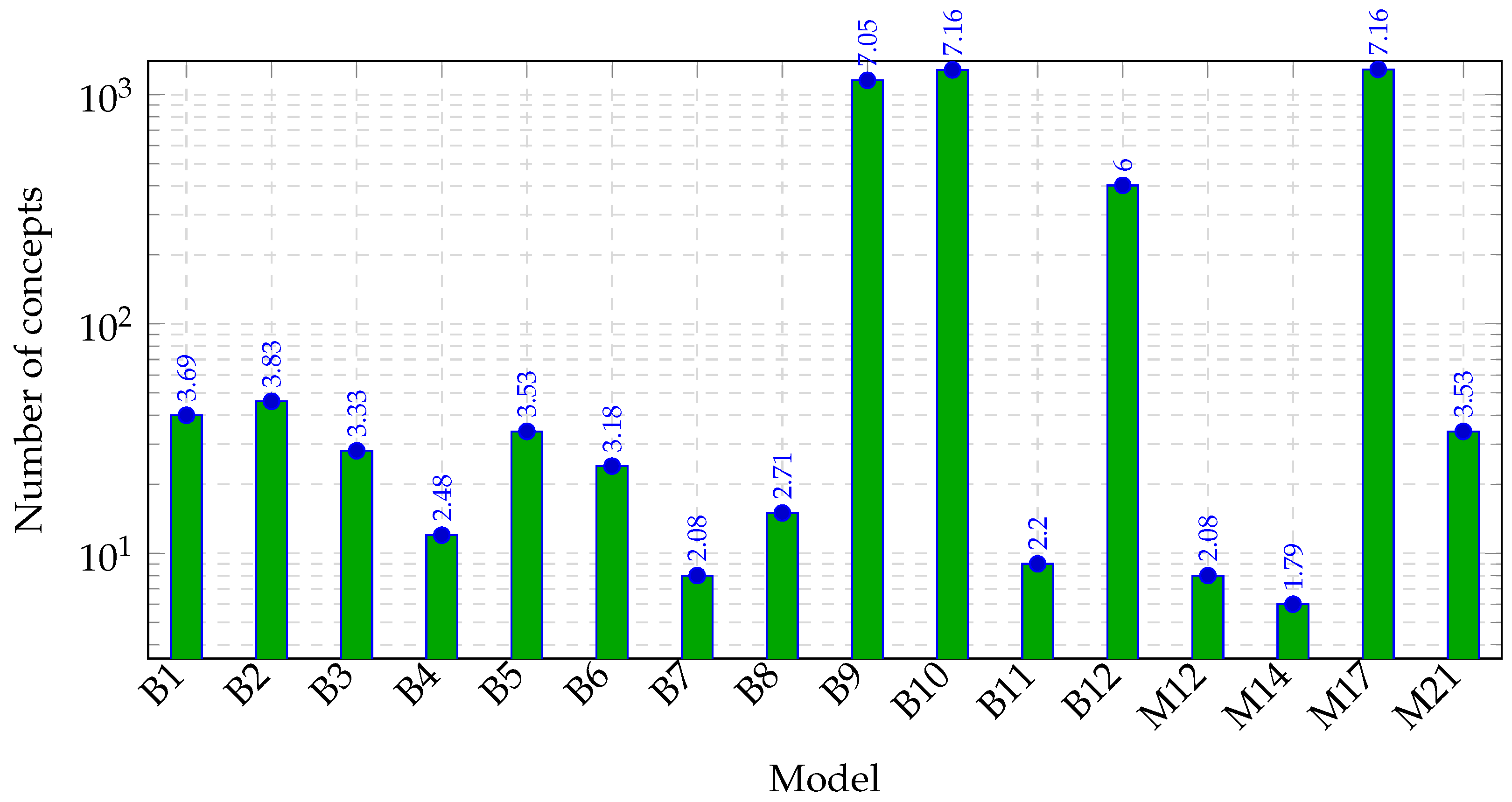
Another important aspect is model complexity (Table 11), which affects performance, required resources, and interpretability/explainability. Figure 16 and Figure 17 compare the number of active weights and concepts across models. The complexity of multimodal FCM models is very high when PCA reduction is not applied; however, when a reduced feature set is used, the number of active weights and concepts decreases significantly.

Table 11. Model complexity comparison across selected data types and training methods.

Method	Data/Variant	Concepts	Weights	Weights ≥ 0.1
Particle swarm optimization	header normalized 0.9 pca	40	1600	1482
Particle swarm optimization	images 0.99 pca	46	2116	1980
Particle swarm optimization	dino 0.9 pca	28	784	702
Gradient descent with centroids	dino siamese 0.9 pca	12	144	102
Simulated annealing	profiles statistical 0.9 pca	34	1156	1056
Gradient descent with centroids	profiles dtw	24	576	484
Gradient descent without centroids	header normalized 0.9 pca	8	64	3
Gradient descent without centroids	images 0.99 pca	15	225	8
Gradient descent without centroids	dino	1154	1,331,716	213
Gradient descent without centroids	dino siamese	1282	1,643,524	250
Gradient descent without centroids	profiles statistical 0.9 pca	9	81	3
Gradient descent without centroids	profiles dtw	402	161,604	202
Two-stage FCM	M12	8	64	8
Two-stage FCM	M14	6	36	4
Multimodal FCM	M17	1288	1,658,944	213
Multimodal FCM	M21	34	1156	4

Figure 16. Comparison of total and active weights across models (log scale).

Figure 17. Comparison of the number of concepts across models (log scale).

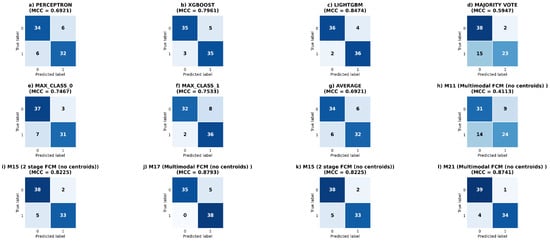
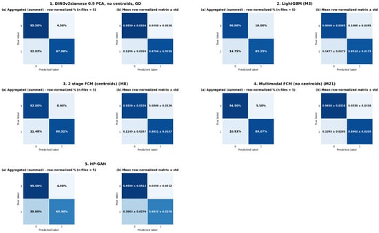
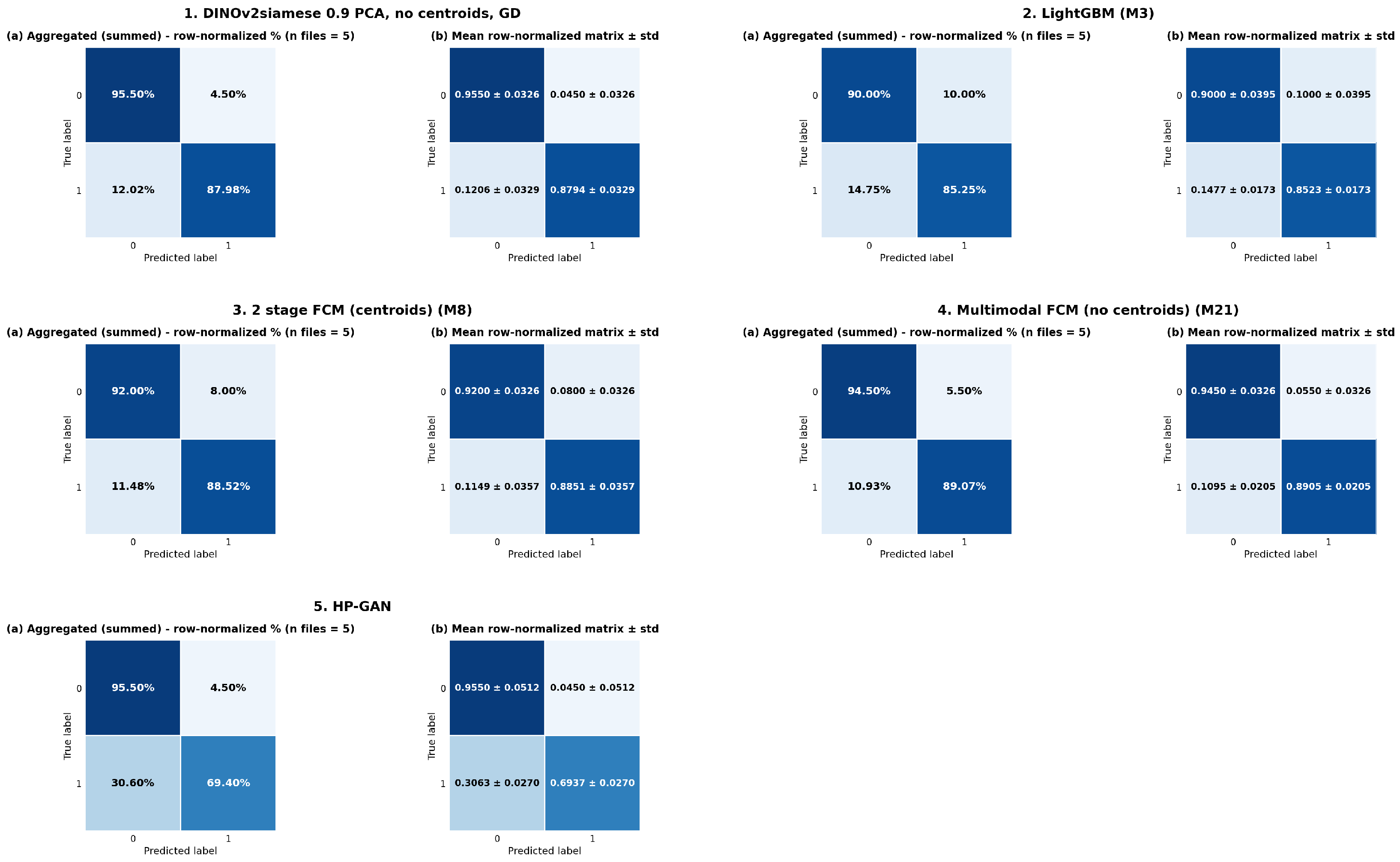
To visualize the results, we prepared confusion matrices for selected models on the hold-out test set (Figure 18) and for 5-fold cross-validation (Figure 19). Achieving 100% prediction accuracy for one class (0% false negatives or 0% false positives) remains an open challenge; however, some models achieve performance close to this level.

Figure 18. Confusion matrices for selected multi-classifiers. The values represent the number of predicted samples per class. For clarity, the class labels are represented by the values 0 and 1, where 0 denotes OK and 1 denotes Porosity.

Figure 19. Confusion matrices for selected models and 5-fold cross-validation. The values represent: (a) percentages of classified samples for each label; (b) the normalized number of classified samples per label, with standard deviation. For clarity, the class labels are represented by the values 0 and 1, where 0 denotes OK and 1 denotes Porosity.

The proposed methods and classifiers are intended for preliminary screening rather than as replacements for more time-consuming inspection procedures. The confusion matrices show that the false-negative rate is higher than 0%, indicating that some samples labeled as Porosity may not be detected by the proposed approach. For M21, the aggregated false-negative rate is approximately 10.95%. Therefore, a trade-off remains between detecting potentially defective parts and reducing the number of parts requiring further investigation. This issue will be further investigated in future work.

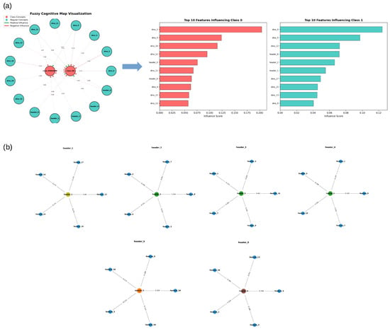
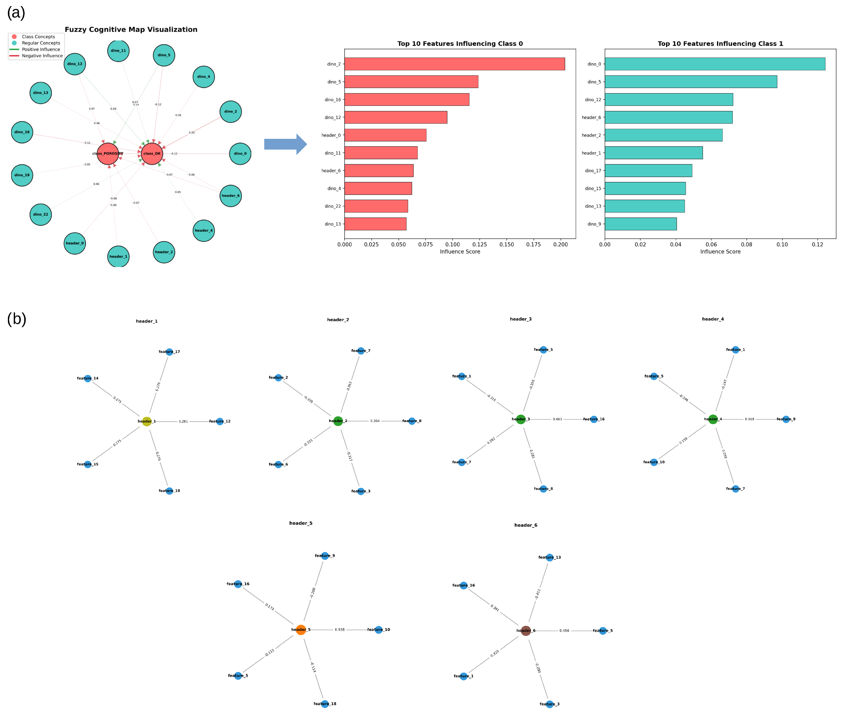
One advantage of using a Fuzzy Cognitive Map is improved explainability compared to deep learning approaches such as HP-GAN. Figure 20 shows an example visualization. The map highlights which features are most important and how they influence the output classification (Figure 20a). Since the input features for the FCM were transformed using PCA, they can also be mapped back to the original features using the corresponding loadings (Figure 20b). However, the weights and connections in the map represent relationships learned by the model and should not be interpreted as causal relationships or as direct evidence of physical mechanisms in the HPDC process. Similarly, the PCA-based features are derived from the original input features (e.g., process parameters).

Figure 20. Fuzzy Cognitive Map visualization for the model achieving the highest MCC: (a) FCM map showing the most influential concepts and their weights, together with the ten most influential features; (b) mapping of the six most influential original input features onto the PCA-based features used by the FCM for header data.

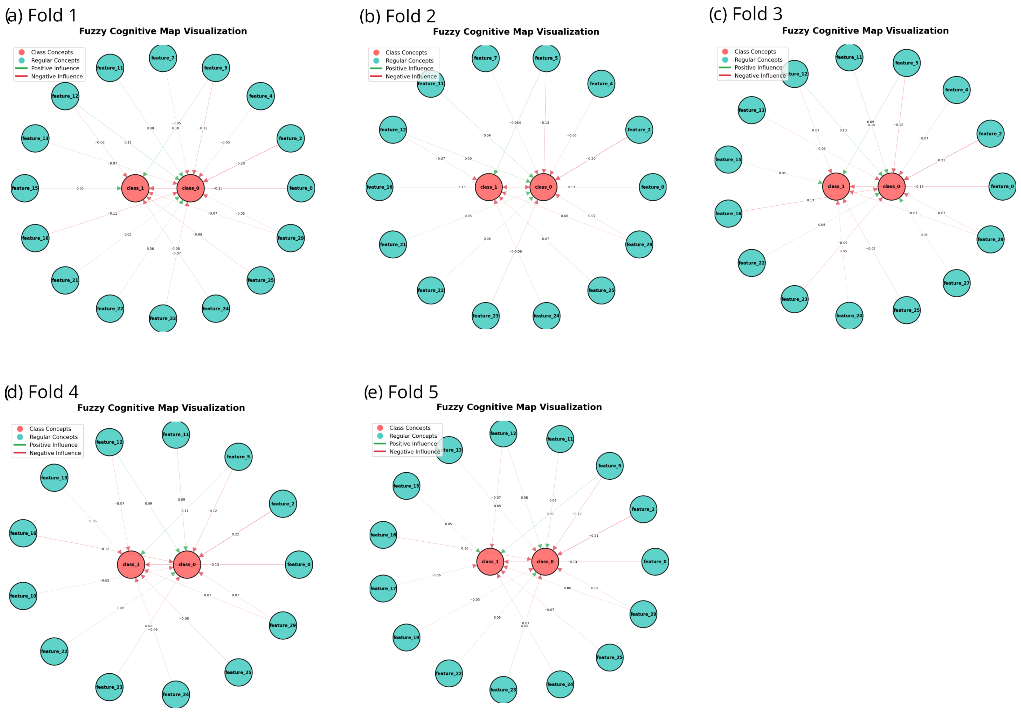
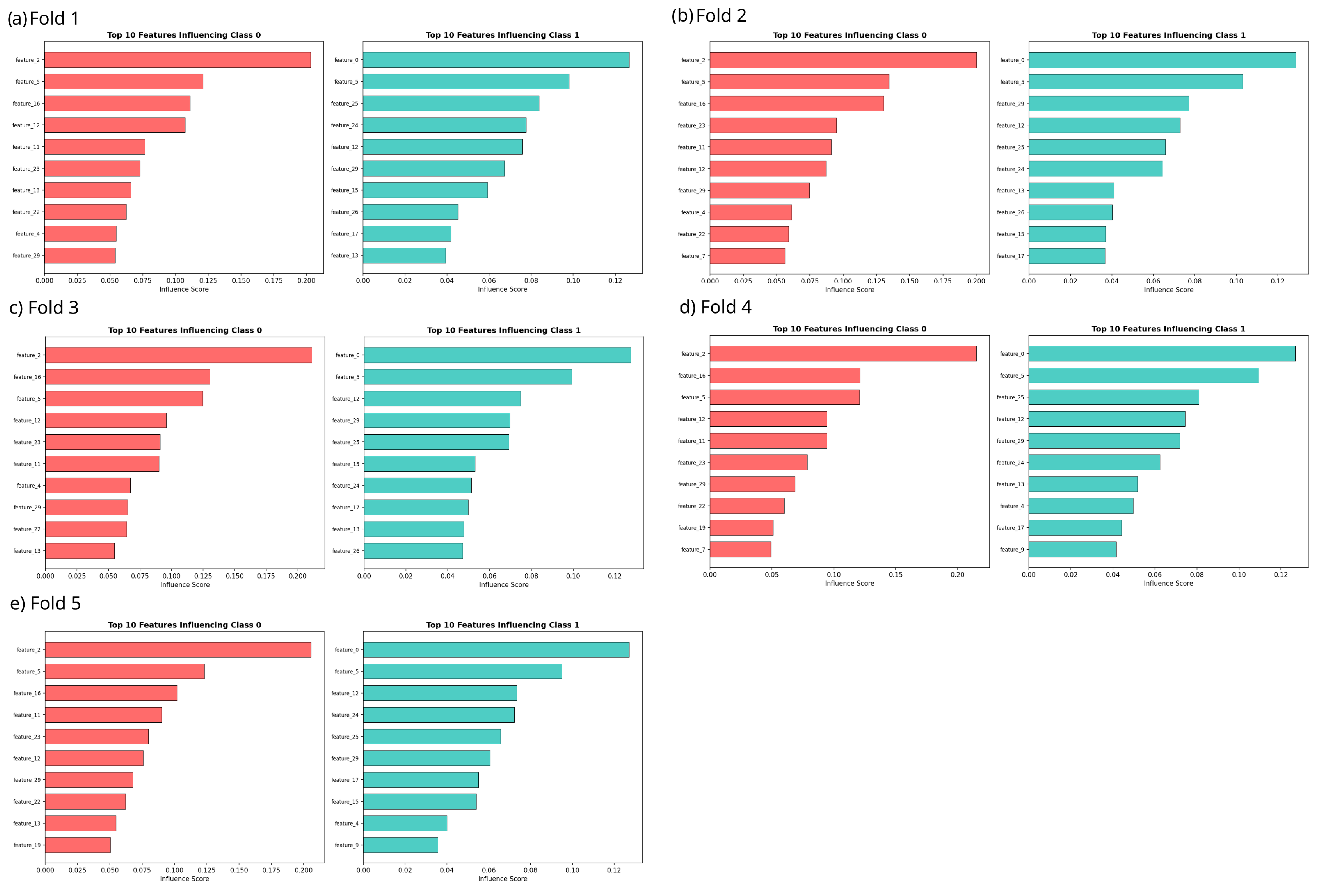
To further demonstrate explainability, we provide two additional visualizations: Figure 21 shows FCM maps with the most important concepts and their weights, while Figure 22 presents the ten most important original features. Both figures show results for the same multimodal model (M21) across all five cross-validation folds. The features represent the model input variables, which correspond to the PCA components obtained from the original feature space. Even though the exact feature ranking varies slightly between folds, many influential features appear consistently, suggesting that the observed feature importance is not limited to a single train–validation split.

Figure 21. Fuzzy Cognitive Map visualizations showing the most influential concepts and their weights for the M21 model across the five cross-validation folds.

Figure 22. The ten most influential features for the M21 model across the five cross-validation folds. The features represent the model input variables, which correspond to the PCA components.

All previously reported cross-validation results were obtained using PCA fitted on the original training set and were retained for consistency with the original experimental protocol. Additionally, Table 12 and Table 13 provide results obtained with PCA and the DINOv2-Siamese feature extractor fitted or trained independently within each training fold and subsequently applied to the corresponding validation fold. In particular, the DINOv2-Siamese model without PCA and the multimodal M21 model achieved comparable MCC values under both protocols, while the LightGBM baseline also showed very similar performance. A more pronounced difference was observed for the DINOv2-Siamese model with PCA, indicating that fold-specific PCA fitting can have a substantial effect for this particular configuration. For the results obtained on the training portions of the folds (Table 13), similar trends to those observed previously can be seen: the training–validation performance gap for the FCM models is relatively small, whereas it is substantially larger for LightGBM. The perfect training performance obtained by LightGBM, with a value of $1.0000$ for all reported metrics, may further indicate potential overfitting.

Table 12. Five-fold cross-validation results for the selected models and the HP-GAN baseline using fold-specific training and preprocessing. For the DINOv2-Siamese models, the feature extractor and PCA were trained or fitted independently using only the training portion of each fold. Values are reported as the mean ± standard deviation.

Model	Method	Performance Metric
		MCC	Balanced Accuracy	F1 Score OK	F1 Score Porosity	Recall OK	Recall Porosity
-	DINOv2-Siamese, no PCA, no centroids, GD	$0.8067\pm 0.0908$	$0.8991\pm 0.0508$	$0.9082\pm 0.0408$	$0.8903\pm 0.0601$	$0.9250\pm 0.0468$	$0.8731\pm 0.1175$
-	DINOv2-Siamese, PCA 0.9, no centroids, GD	$0.7147\pm 0.0655$	$0.8541\pm 0.0342$	$0.8684\pm 0.0290$	$0.8416\pm 0.0396$	$0.9050\pm 0.0274$	$0.8032\pm 0.0591$
M3.5	LightGBM (initial inputs)	$0.8764\pm 0.0709$	$0.9364\pm 0.0367$	$0.9410\pm 0.0345$	$0.9330\pm 0.0388$	$0.9550\pm 0.0447$	$0.9179\pm 0.0588$
M21	Multimodal FCM (no centroids)	$0.8234\pm 0.0427$	$0.9105\pm 0.0207$	$0.9154\pm 0.0225$	$0.9063\pm 0.0208$	$0.9250\pm 0.0468$	$0.8959\pm 0.0242$
	HP-GAN (header and images)	$0.6791\pm 0.0665$	$0.8243\pm 0.0285$	$0.8542\pm 0.0281$	$0.7965\pm 0.0307$	$0.9550\pm 0.0512$	$0.6937\pm 0.0270$

Table 13. Five-fold cross-validation results for the selected models evaluated on the training portions of the respective folds. Values are reported as the mean ± standard deviation.

Model	Method	Performance Metric
		MCC	Balanced Accuracy	F1 Score OK	F1 Score Porosity	Recall OK	Recall Porosity
-	DINOv2-Siamese, no PCA, no centroids, GD	$0.8015\pm 0.0368$	$0.8961\pm 0.0263$	$0.9053\pm 0.0156$	$0.8874\pm 0.0355$	$0.9300\pm 0.0462$	$0.8623\pm 0.0963$
-	DINOv2-Siamese, PCA 0.9, no centroids, GD	$0.7221\pm 0.0221$	$0.8593\pm 0.0112$	$0.8708\pm 0.0101$	$0.8495\pm 0.0123$	$0.8975\pm 0.0095$	$0.8211\pm 0.0152$
M3.5	LightGBM (initial inputs)	$1.0000\pm 0.0000$	$1.0000\pm 0.0000$	$1.0000\pm 0.0000$	$1.0000\pm 0.0000$	$1.0000\pm 0.0000$	$1.0000\pm 0.0000$
M21	Multimodal FCM (no centroids)	$0.8459\pm 0.0164$	$0.9214\pm 0.0060$	$0.9267\pm 0.0086$	$0.9173\pm 0.0053$	$0.9425\pm 0.0355$	$0.9003\pm 0.0242$

4. Conclusions

In this paper, we address the problem of early porosity detection in the High-Pressure Die Casting process in a real industrial use case. The proposed approach incorporates multiple data sources, including sensor readouts from the HPDC machine, time-series data, and thermal images. The main classifiers are Fuzzy Cognitive Maps (FCMs), which offer a higher level of interpretability than neural networks. Building on our previous work [36], we introduced new feature extractors, classification variants, and weight-selection strategies. For thermal images, we investigated a foundation model (DINOv2) to mitigate training-related issues and evaluated its effectiveness. In addition, we analyzed how PCA-based feature-space reduction influences classification performance. We also investigated the efficiency of different training algorithms and their relationship to model complexity. Furthermore, using an example, we demonstrated how the proposed model supports the explainability of results and decisions. Finally, we compared our approach with the HP-GAN algorithm [31] and showed that our approach achieves higher performance while maintaining high interpretability. However, the multimodal data fusion needs further investigation, as the results did not prove that it can substantially improve the performance. It must be noted that the results and conclusions about the multimodal fusion are restricted only to the evaluated configurations.

Future work will focus on method improvements, particularly on developing and evaluating a two-layer FCM approach with weight-calculation and concept-selection algorithms tailored to its structure. Moreover, we plan to conduct additional experiments on a larger dataset to assess robustness, scalability, and generalization. We will also further improve the analysis of time-series data, including the use of time-series-specific models.

Another important research direction is to investigate the HPDC process in more detail to evaluate how time-varying features provide additional information for more reliable defect detection. In addition, we will explore alternative fusion strategies across data sources to improve classification performance. Relating predictive results to the underlying physical mechanisms would also be valuable.

Finally, we will further reduce model complexity to enable faster inference without sacrificing performance, which is important for online monitoring. We also plan to improve explainability to better understand relationships among process parameters, extracted features, and the final classification. Furthermore, we will investigate applying the proposed method to other industrial use cases (e.g., welding).

References

- Liu, W.; Peng, T.; Kishita, Y.; Umeda, Y.; Tang, R.; Tang, W.; Hu, L. Critical life cycle inventory for aluminum die casting: A lightweight-vehicle manufacturing enabling technology. Appl. Energy 2021, 304, 117814. [Google Scholar] [CrossRef] [Scilit]
- Gonçalves, M.; Jolly, M.R.; Salonitis, K.; Pagone, E. Resource Efficiency Analysis of High Pressure Die Casting Process. In Light Metals 2018; Martin, O., Ed.; Springer: Cham, Swizterland, 2018; pp. 1041–1047. [Google Scholar]
- Shyam, A.; Plotkowski, A.; Wang, Q.; Wang, A.; Bahl, S.; Rakhmonov, J.; Hartlieb, M.; Yang, Y.; Richter, N.; Knapp, G.; et al. Alloy design for sustainable aluminum high pressure die castings: A review. Int. Mater. Rev. 2026. [Google Scholar] [CrossRef] [Scilit]
- Gariboldi, E.; Bonollo, F.; Rosso, M. Proposal of a Classification of Defects of High-pressure Diecast Products. Metall. Ital. 2007. Available online: https://www.fracturae.com/index.php/aim/article/view/516 (accessed on 29 August 2026).
- Lee, S.; Han, D.; Kang, S.; Kim, N. Method of predicting shrinkage defects and deriving process conditions in HPDC (high-pressure die-casting) for electric vehicle motor housings. Int. J. Met. 2024, 18, 1262–1272. [Google Scholar] [CrossRef] [Scilit]
- Kang, H.-J.; Yoon, P.-H.; Lee, G.-H.; Park, J.-Y. Effects of porosity on mechanical properties of castings in high-pressure die-casting process. Int. J. Met. 2025, 19, 2918–2927. [Google Scholar] [CrossRef] [Scilit] [PubMed]
- Lee, S.; Gokhale, A.; Patel, G.; Evans, M. Effect of process parameters on porosity distributions in high-pressure die-cast AM50 Mg-alloy. Mater. Sci. Eng. A 2006, 427, 99–111. [Google Scholar] [CrossRef] [Scilit]
- Lee, S.G.; Gokhale, A.M. Formation of gas induced shrinkage porosity in Mg-alloy high-pressure die-castings. Scr. Mater. 2006, 55, 387–390. [Google Scholar] [CrossRef] [Scilit]
- Klym, H.; Karbovnyk, I.; Piskunov, S.; Popov, A.I. Positron Annihilation Lifetime Spectroscopy Insight on Free Volume Conversion of Nanostructured MgAl2O4 Ceramics. Nanomaterials 2021, 11, 3373. [Google Scholar] [CrossRef] [Scilit] [PubMed]
- Shpotyuk, O.; Ingram, A.; Boussard-Pledel, C.; Bureau, B.; Lukáčová Bujňáková, Z.; Baláž, P.; Mahlovanyi, B.; Shpotyuk, Y. The Art of Positronics in Contemporary Nanomaterials Science: A Case Study of Sub-Nanometer Scaled Glassy Arsenoselenides. Materials 2022, 15, 302. [Google Scholar] [CrossRef] [Scilit] [PubMed]
- Brůna, M.; Medňanský, M.; Matejka, M.; Podprocká, R. Influence of HPDC Process Parameters on the Microstructure of EC Electromotor Housing. Metals 2023, 13, 295. [Google Scholar] [CrossRef] [Scilit]
- Zhang, Y.; Lordan, E.; Dou, K.; Wang, S.; Fan, Z. Influence of porosity characteristics on the variability in mechanical properties of high pressure die casting (HPDC) AlSi7MgMn alloys. J. Manuf. Process. 2020, 56, 500–509. [Google Scholar] [CrossRef] [Scilit]
- Lee, S.; Patel, G.; Gokhale, A.; Sreeranganathan, A.; Horstemeyer, M. Quantitative fractographic analysis of variability in the tensile ductility of high-pressure die-cast AE44 Mg-alloy. Mater. Sci. Eng. A 2006, 427, 255–262. [Google Scholar] [CrossRef] [Scilit]
- Yamada, Y.; Yoshii, H.; Mochizuki, S.; Bannai, Y.; Yaokawa, J.; Anzai, K.; Oikawa, K. Evaluation of J Factor and Leakage Quality for High Pressure Die Casting Applied to Closed-deck Type Cylinder Block. In Proceedings of the Small Engine Technology Conference & Exposition, Sapporo, Japan, 8 November 2011. [Google Scholar] [CrossRef] [Scilit]
- Wilczek, A.; Długosz, P.; Hebda, M. Porosity Characterization of Aluminium Castings by Using Particular Non-destructive Techniques. J. Nondestruct. Eval. 2015, 34, 26. [Google Scholar] [CrossRef] [Scilit]
- Nourian-Avval, A.; Fatemi, A. Characterization and Analysis of Porosities in High Pressure Die Cast Aluminum by Using Metallography, X-Ray Radiography, and Micro-Computed Tomography. Materials 2020, 13, 3068. [Google Scholar] [CrossRef] [Scilit] [PubMed]
- Wan, Q.; Zhao, H.; Zou, C. Effect of Micro-porosities on Fatigue Behavior in Aluminum Die Castings by 3D X-ray Tomography Inspection. ISIJ Int. 2014, 54, 511–515. [Google Scholar] [CrossRef] [Scilit]
- Maierhofer, C.; Myrach, P.; Röllig, M.; Jonietz, F.; Illerhaus, B.; Meinel, D.; Richter, U.; Miksche, R. Characterization of pores in high pressure die cast aluminum using active thermography and computed tomography. AIP Conf. Proc. 2016, 1706, 110009. [Google Scholar] [CrossRef] [Scilit]
- Disselhoff, T.; Martin, R.J. Data-Driven Early Quality Prediction in High Pressure Die Casting. Int. J. Met. 2026, 20, 1897–1907. [Google Scholar] [CrossRef] [Scilit]
- Pachandrin, S.; Hoffmann, N.; Dilger, K.; Rokicki, M.; Niederée, C.; Stürenburg, L.; Noske, H.; Denkena, B.; Kallisch, J.; Wunck, C. Data-Driven Prediction of Casting Defects in Magnesium High-Pressure Die Casting Using Machine Learning. Int. J. Met. 2026, 20, 112–131. [Google Scholar] [CrossRef] [Scilit]
- Qiao, Q.; Hu, H.; Ahmad, A.; Wang, K. A Review of Metal Surface Defect Detection Technologies in Industrial Applications. IEEE Access 2025, 13, 48380–48400. [Google Scholar] [CrossRef] [Scilit]
- Lv, X.; Duan, F.; Jiang, J.-J.; Fu, X.; Gan, L. Deep Metallic Surface Defect Detection: The New Benchmark and Detection Network. Sensors 2020, 20, 1562. [Google Scholar] [CrossRef] [Scilit] [PubMed]
- Ziółkowski, G.; Chlebus, E.; Szymczyk, P.; Kurzac, J. Application of X-ray CT method for discontinuity and porosity detection in 316L stainless steel parts produced with SLM technology. Arch. Civ. Mech. Eng. 2014, 14, 608–614. [Google Scholar] [CrossRef] [Scilit]
- Williams, J.; Dryburgh, P.; Clare, A.; Rao, P.; Samal, A. Defect Detection and Monitoring in Metal Additive Manufactured Parts through Deep Learning of Spatially Resolved Acoustic Spectroscopy Signals. Smart Sustain. Manuf. Syst. 2018, 2, 204–226. [Google Scholar] [CrossRef] [Scilit]
- Huang, Y.; Wu, D.; Zhang, Z.; Chen, H.; Chen, S. EMD-based pulsed TIG welding process porosity defect detection and defect diagnosis using GA-SVM. J. Mater. Process. Technol. 2017, 239, 92–102. [Google Scholar] [CrossRef] [Scilit]
- Lee, J.H.; Noh, S.D.; Kim, H.J.; Kang, Y.S. Implementation of Cyber-Physical Production Systems for Quality Prediction and Operation Control in Metal Casting. Sensors 2018, 18, 1428. [Google Scholar] [CrossRef] [Scilit] [PubMed]
- Plentz, P.D.M.; Ribeiro, T.M.M.; Rahmig, H.F.C.; Bulcão-Neto, R.F.; Sene, I.G.; Morales, A.S. Digital Transformation: Challenges About Iot and Ai in High Pressure Die Casting (HPDC). In Proceedings of the 2025 IEEE 19th International Symposium on Applied Computational Intelligence and Informatics (SACI), Timisoara, Romania, 19–24 May 2025; pp. 1–6. [Google Scholar] [CrossRef] [Scilit]
- Gupta, R.; Anand, V.; Gupta, S.; Koundal, D. Deep learning model for defect analysis in industry using casting images. Expert Syst. Appl. 2023, 232, 120758. [Google Scholar] [CrossRef] [Scilit]
- Andriosopoulou, G.; Mastakouris, A.; Masouros, D.; Benardos, P.; Vosniakos, G.C.; Soudris, D. Defect Recognition in High-Pressure Die-Casting Parts Using Neural Networks and Transfer Learning. Metals 2023, 13, 1104. [Google Scholar] [CrossRef] [Scilit]
- Jakumeit, J.; Behnken, H.; Laqua, R.; Mbewou, S.; Fehlbier, M.; Gänz, J.; Becker, L. Coupled Modeling of Misrun, Cold Shut, Air Entrainment, and Porosity for High-Pressure Die Casting Applications. Miner. Met. Mater. Ser. 2021, 6, 865–870. [Google Scholar] [CrossRef] [Scilit]
- Kim, J.; Park, C.; Park, W.; Park, Y.; Cho, C.; Kim, D. A Study on High Pressure Die-Casting Defect Prediction Deep Learning Algorithm for Porosity Defect Detection based on Process Parameters and Thermal Image. Korean J. Comput. Des. Eng. 2023, 28, 222–231. [Google Scholar] [CrossRef] [Scilit]
- Sovatzidi, G.; Vasilakakis, M.D.; Iakovidis, D.K. Automatic Fuzzy Graph Construction for Interpretable Image Classification. In Proceedings of the International Conference on Image Processing (ICIP), Bordeaux, France, 16–19 October 2022; pp. 3743–3747. [Google Scholar] [CrossRef] [Scilit]
- Tziolas, T.; Papageorgiou, K.; Feleki, A.; Theodosiou, T.; Rapti, K.; Papageorgiou, E.; Pantoja, S.; Cuinas, A. Deep Fuzzy Cognitive Maps for Defect Inspection in Antenna Assembly. Procedia Comput. Sci. 2024, 232, 97–106. [Google Scholar] [CrossRef] [Scilit]
- Vasilakakis, M.; Sovatzidi, G.; Dimas, G.; Iakovidis, D.K. Towards the Interpretation of Convolutional Neural Networks for Image Classification Using Fuzzy Sets. In Proceedings of the IEEE International Conference on Systems, Man and Cybernetics, Prague, Czech Republic, 9–12 October 2022; pp. 2912–2917. [Google Scholar] [CrossRef] [Scilit]
- Sovatzidi, G.; Vasilakakis, M.D.; Iakovidis, D.K. Towards the Interpretation of Multi-Label Image Classification Using Transformers and Fuzzy Cognitive Maps. In Proceedings of the IEEE International Conference on Fuzzy Systems, Incheon, Republic of Korea, 13–17 August 2023. [Google Scholar] [CrossRef] [Scilit]
- Michno, T.; Holom, R.; Schmalzer, S.; Meyer-Heye, P.; Scampone, G.; Riegler, E.; Hartmann, M.; Repanšek, U.; Košir, N.; Šifrer, P.; et al. Porosity Classification in High Pressure Die Casting Using Thermal Images and Sensor Data Fusion via Fuzzy Cognitive Maps. In Proceedings of the 21st International Conference on Computer Vision Theory and Applications—Volume 1: VISAPP; INSTICC; SciTePress: Setúbal, Portugal, 2026; pp. 613–622. [Google Scholar] [CrossRef] [Scilit]
- Berndt, D.J.; Clifford, J. Using dynamic time warping to find patterns in time series. In Proceedings of the 3rd International Conference on Knowledge Discovery and Data Mining; AAAIWS’94; AAAI Press: Washington, DC, USA, 1994; pp. 359–370. [Google Scholar]
- Schmalzer, S.; Holom, R.M.; Falkner, D.; Michno, T.; Repanšek, U.; Košir, N.; Šifrer, P. Time Series Classification in High-Pressure Die Casting Manufacturing using Dynamic Time Warping. Procedia Comput. Sci. 2026, 277, 1631–1640. [Google Scholar] [CrossRef] [Scilit]
- Oquab, M.; Darcet, T.; Moutakanni, T.; Vo, H.; Szafraniec, M.; Khalidov, V.; Fernandez, P.; Haziza, D.; Massa, F.; El-Nouby, A.; et al. DINOv2: Learning Robust Visual Features without Supervision. arXiv 2024, arXiv:2304.07193. [Google Scholar] [CrossRef] [Scilit]
- Kosko, B. Fuzzy cognitive maps. Int. J. Man-Mach. Stud. 1986, 24, 65–75. [Google Scholar] [CrossRef] [Scilit]
- Bueno, S.; Salmeron, J.L. Benchmarking main activation functions in fuzzy cognitive maps. Expert Syst. Appl. 2009, 36, 5221–5229. [Google Scholar] [CrossRef] [Scilit]
- ichi Amari, S. Backpropagation and stochastic gradient descent method. Neurocomputing 1993, 5, 185–196. [Google Scholar] [CrossRef] [Scilit]
- Papageorgiou, E.I.; Parsopoulos, K.E.; Stylios, C.S.; Groumpos, P.P.; Vrahatis, M.N. Fuzzy Cognitive Maps Learning Using Particle Swarm Optimization. J. Intell. Inf. Syst. 2005, 25, 95–121. [Google Scholar] [CrossRef] [Scilit]
- Papageorgiou, E.; Stylios, C.; Groumpos, P. Active Hebbian learning algorithm to train fuzzy cognitive maps. Int. J. Approx. Reason. 2004, 37, 219–249. [Google Scholar] [CrossRef] [Scilit]
- Huerga, A.V. A balanced differential learning algorithm in fuzzy cognitive maps. In Proceedings of the 16th International Workshop on Qualitative Reasoning, Barcelona, Spain, 10–12 June 2002; Volume 2002. [Google Scholar]
- Kosko, B. Differential Hebbian learning. AIP Conf. Proc. 1986, 151, 277–282. [Google Scholar] [CrossRef] [Scilit]
- Kirkpatrick, S.; Gelatt, C.D.; Vecchi, M.P. Optimization by Simulated Annealing. Science 1983, 220, 671–680. [Google Scholar] [CrossRef] [Scilit] [PubMed]
- Barata, J.C.A.; Hussein, M.S. The Moore–Penrose Pseudoinverse: A Tutorial Review of the Theory. Braz. J. Phys. 2012, 42, 146–165. [Google Scholar] [CrossRef] [Scilit]
- Stach, W.; Kurgan, L.; Pedrycz, W.; Reformat, M. Genetic learning of fuzzy cognitive maps. Fuzzy Sets Syst. 2005, 153, 371–401. [Google Scholar] [CrossRef] [Scilit]
- Poczeta, K.; Yastrebov, A.; Papageorgiou, E.I. Learning Fuzzy Cognitive Maps using Structure Optimization Genetic Algorithm. Proc. Fed. Conf. Comput. Sci. Inf. Syst. ACSIS 2015, 5, 547–554. [Google Scholar] [CrossRef] [Scilit]
- Measures to Guarantee Valuable Validation Results. MetaFacturing Project, Grant Agreement No. 101091635. Public Deliverable. Available online: https://cordis.europa.eu/project/id/101091635/results (accessed on 18 September 2026).
- Gorodkin, J. Comparing two K-category assignments by a K-category correlation coefficient. Comput. Biol. Chem. 2004, 28, 367–374. [Google Scholar] [CrossRef] [Scilit] [PubMed]
- Chicco, D.; Jurman, G. The advantages of the Matthews correlation coefficient (MCC) over F1 score and accuracy in binary classification evaluation. BMC Genom. 2020, 21, 6. [Google Scholar] [CrossRef] [Scilit] [PubMed]
Disclaimer/Publisher’s Note: The statements, opinions and data contained in all publications are solely those of the individual author(s) and contributor(s) and not of MDPI and/or the editor(s). MDPI and/or the editor(s) disclaim responsibility for any injury to people or property resulting from any ideas, methods, instructions or products referred to in the content. |
© 2026 by the authors. Licensee MDPI, Basel, Switzerland. This article is an open access article distributed under the terms and conditions of the Creative Commons Attribution (CC BY) license.