


Abstract
Road authorities increasingly use machine-learning models to rank high-risk locations and to allocate scarce safety resources. These models are almost always judged by their predictive accuracy on a random hold-out sample. This study shows that practice hides an important risk. We evaluate crash-severity models the way they are used in practice. Each model is trained on past data and applied to later years. We measure decision quality, not only accuracy. The data include 45,288 police-reported crashes recorded across all thirteen administrative regions of Saudi Arabia between 2016 and 2021. Four results follow. First, decision quality decays much faster than accuracy. Over a three-year deployment gap, the area under the curve falls by less than two percent. Yet the overlap between the predicted and the true high-risk sites falls from 0.44 to 0.24, close to the value expected by chance. Second, the useful shelf life of a model is short. Site rankings approach random within about two to three years. Third, retraining recovers only a small part of the lost decision quality, at most about three percentage points of overlap. Fourth, the standard drift detector, the Population Stability Index on the score distribution, never crosses its alert threshold during this decay across eighteen design settings. A decision-aware monitor based on turnover in the model’s own high-risk set instead reveals churn of 0.20 to 0.60 from the same deployment-time data. Fifth, model selection also changes under decision-level evaluation. Ranking candidate models by accuracy and by decision quality disagree, with a rank correlation near zero, so the most accurate model is not the best decision-level performer. Standard accuracy-and-drift practice therefore misleads at both the selection and the monitoring stage. Crash-severity models should be evaluated and monitored at the level of the decisions they inform.
1. Introduction
Road traffic crashes remain a leading cause of death and serious injury worldwide. About 1.19 million people die on the roads each year. Road traffic injury is the leading killer of children and young people aged 5 to 29 years [1]. Low- and middle-income countries carry a large share of this burden [1]. Understanding the factors that raise the severity of a crash is therefore central to road-safety research and practice.
Over the past decade, the methods used to study crash-injury severity have changed. Traditional discrete-outcome models once dominated the field. These include ordered and unordered logit and probit models [2,3]. Such models remain valuable because their coefficients are easy to interpret. However, they require the analyst to specify the functional form in advance. Machine-learning methods relax that requirement. They capture non-linear effects and interactions among crash factors without prior specification [4,5]. Recent work comparing deep-learning and advanced statistical models cautions, however, that superior predictive metrics do not guarantee correct inference. Estimated variable effects from deep learning can be inconsistent in magnitude and occasionally in direction, with the plausible values produced by statistical models. The same work also documents statistically significant shifts in model parameters over time [6]. Gradient-boosted decision-tree models, in particular, are now widely used for crash-severity prediction [7,8]. Ensemble approaches have also been applied to accident-consequence prediction in other transport modes, such as hybrid ensemble models for urban rail transit incidents [9].
These models are not built only for academic interest. Their stated aim is to support road-safety practice [6,7]. They identify the factors and the locations linked to severe outcomes. Authorities then target enforcement, prioritise engineering treatments, and allocate limited safety budgets. A crash-severity model is therefore a tool for deployment. It is estimated on historical records. It is then applied to a future that has not yet been observed.
This intended use sits uneasily with two facts. Both facts are well established, but in separate research streams. The first fact concerns evaluation. Crash-severity models are almost always judged by their accuracy on a random hold-out sample [10]. A random split mixes observations from different periods. It therefore cannot show how a model behaves when applied forward in time. The second fact concerns the data. The crash-severity process is not stationary. A large body of work shows that the effects of contributing factors shift across time periods. This property is known as temporal instability [11,12]. If the process drifts, and if models are still judged in a way that hides drift, then the reported performance may overstate deployed behaviour.
The consequences of temporal instability for deployed models have received little attention. Econometric literature treats instability as an estimation problem [11]. It does not ask what the drift does to the decisions a deployed model produces. Machine-learning literature builds and deploys such models. Yet it rarely tests for instability. A separate field, machine-learning operations, offers concept-drift detectors. These flag when a deployed model’s environment has changed [13,14]. However, the most common detectors watch statistical distributions rather than decisions. A theoretical result shows that such detectors can miss drift that is relevant to the decision boundary [14]. Whether this limitation matters for crash-severity models has not been examined.
These gaps matter because the decision a crash-severity model supports is specific and consequential. In road-safety management, the standard task is network screening. The analyst ranks locations by estimated risk. The output is a list of the most hazardous sites [15,16]. Resources are then directed to the top of that list. The quality of the ranking, and its stability over time, is the substance of the decision [15]. A model whose accuracy is stable but whose high-risk list has drifted will send resources to the wrong places. An evaluation that reports only accuracy will not reveal this.
This study addresses the combined gap. It evaluates crash-severity models under deployment-realistic conditions. Each model is trained on past data. It is then applied to later years. The study asks four research questions.
RQ1.
When a crash-severity model is applied forward in time, does the quality of its location-level decisions decay faster than its aggregate predictive accuracy?
RQ2.
How quickly does decision quality decay, that is, what is the effective deployment shelf life of a crash-severity model?
RQ3.
Do common retraining strategies restore the lost decision quality, and at what retraining cost?
RQ4.
Does the standard model-drift detector used in practice alert practitioners to this decay, and if not, what monitoring procedure would?
The empirical setting is Saudi Arabia. It is a large and rapidly motorising country in which road safety is a national priority [7]. We analysed 45,288 police-reported crashes recorded across all thirteen administrative regions between October 2016 and February 2021. The four calendar years 2017 to 2020 provide the full-coverage window used for the forward-in-time analysis.
The contribution of the paper is integrative rather than algorithmic. It introduces no new prediction method and no new drift statistic. Instead, it connects four research streams that have developed apart. These are machine-learning crash-severity modelling, temporal instability in road-safety analysis, concept drift in deployed machine learning, and network screening for safety management. In doing so, it reveals a deployment risk that each stream, on its own, is likely to miss. The practical message is a shift in how crash-severity models are assessed. The shift moves away from aggregate accuracy on random splits. It moves toward decision-level performance under forward-in-time deployment, supported by decision-aware monitoring.
Throughout this paper, we distinguish two levels of performance, and the distinction is central to the argument. Predictive accuracy refers to how well a model classifies the severity of individual crashes and is measured by the area under the receiver operating characteristic curve. Decision quality refers to how well the model supports the operational decision it is built to inform, namely the correct identification of the highest-risk locations for treatment. It is measured by the overlap between the model’s top-ranked sites and the truly highest-risk sites and by the rank correlation between the predicted and realised site orderings. The two are distinct. Accuracy is computed over all crashes and is dominated by the stable low-risk majority. Decision quality depends only on the ordering of the high-risk tail, which is what resource allocation acts upon. Where we refer to decision quality, we mean this location-ranking quality, not a property of the algorithm in the abstract.
2. Background and Related Work
This study draws on four research streams. These are machine-learning models for crash-severity prediction, temporal instability in road-safety analysis, concept drift and model monitoring in deployed machine learning, and forward-in-time validation together with network screening. Each stream is reviewed in turn. The section then states the gap that the paper addresses.
2.1. Machine-Learning Models for Crash-Severity Prediction
Crash-severity analysis has shifted from parametric discrete-outcome models toward machine learning. The parametric approach uses ordered and unordered logit and probit models and their random-parameters extensions [2,17]. These models are interpretable. They also require the analyst to assume a functional form, an error distribution, and the interaction terms. Machine-learning methods avoid these assumptions. They represent non-linear effects and high-order interactions directly from the data [4,5].
Among machine-learning methods, tree-based ensembles have become the standard choice. Gradient-boosted decision trees perform especially well. Common implementations are Extreme Gradient Boosting, the Light Gradient Boosting Machine, and Categorical Boosting [4,16]. Comparative studies repeatedly report that boosted-tree models outperform single-tree models and logistic regression. Aldhari et al. [7] compared random forest, Extreme Gradient Boosting, and logistic regression on crash data from Qassim Province, and the boosted-tree model performed best. Alanazi and Okail [8] evaluated six tree-based learners on crashes in Jeddah, and Extreme Gradient Boosting again performed best, reaching an area under the curve of 0.92. Niyogisubizo et al. [18] combined balanced bagging with a gradient-boosting learner to address class imbalance.
Two further themes recur in this literature. The first is class imbalance. Severe crashes are a small minority of all crashes. A model trained on the raw distribution tends to under-predict them. Recent studies therefore pair boosted-tree learners with resampling methods [7,18]. The second theme is interpretability. Tree ensembles are not transparent. The SHapley Additive exPlanations framework, known as SHAP, has become a standard companion [19]. It recovers the global and local contribution of each predictor. In crash-severity work, SHAP consistently highlights excess speed, driver behaviour, adverse weather, and collision type [8].
This template has been applied across many settings. Recent studies model driver-injury severity on mountainous roads [20,21]. Others model pedestrian-injury severity [22]. Work specific to Saudi Arabia follows the same pattern. Jamal and Umer [23] applied a neural network to rural highways. Aldhari et al. [7] modelled crashes in Qassim Province. Alanazi and Okail [8] modelled crashes in Jeddah. Alanazi et al. [24] compared deep-learning and traditional models across fourteen cities in the Eastern Province.
Two features of this literature motivate the present study. First, model quality is almost always reported as a single number on a random hold-out sample. The number is usually accuracy, the F1 score, or the area under the curve. A random partition ignores time. Second, the stated purpose is prospective. The studies aim to guide future safety decisions. There is a clear gap between a static evaluation and a forward-looking use.
2.2. Temporal Instability in Crash-Severity Analysis
A large body of work in road-safety econometrics studies temporal instability. The term means that the effects of crash factors are not constant over time. A coefficient estimated for one period may differ from the coefficient for the same factor in another period. If the relationships shift, then a pooled model hides the shift. A model estimated on one period may mislead when applied to another.
Mannering [11] consolidated this agenda in a review. The review argued that temporal shifts in factor effects are common. It also argued that ignoring them yields biased estimates and poor policy inferences. The review built on earlier work on unobserved heterogeneity [17]. Temporal instability can be seen as a time-indexed form of that broader problem.
The empirical evidence is consistent. Malyshkina and Mannering [25] found that the factors affecting severity changed even week to week. Behnood and Mannering [10] tested the stability of driver-injury factors in single-vehicle crashes and found significant instability. Later work extended the analysis to pedestrians, trucks, and motorcyclists and to changes in speed limits [26,27,28]. Recent evidence confirms that instability is detectable over short windows: using four years of state highway crash data, statistically significant temporal instability was found at the five percent level, requiring year-specific models [29]. This matters for deployment because it indicates that the relationships a model encodes can shift well within the interval over which such models are typically left in service. The standard method is now well defined. Analysts use likelihood-ratio tests to compare pooled and period-specific models. They use random-parameters models to absorb unobserved heterogeneity. Hou et al. [30] discussed out-of-sample prediction and temporal testing for such models.
Two features of this literature matter here. First, the evidence is concentrated in North America, Europe, and East Asia. Temporal-stability testing is rare in the Middle East and North Africa. Second, and more important, instability is treated as an estimation concern. The literature shows that the process moves. It does not ask what that movement does to the decisions a deployed model produces year after year. The machine-learning literature in Section 2.1 builds and deploys such models but does not test for instability. The econometric literature documents the instability but does not follow it to deployment. The present paper connects the two.
2.3. Concept Drift and Model Monitoring in Deployed Machine Learning
The machine-learning community studies the same phenomenon under a different name. A model learned from past data may lose accuracy when the world changes. A change in the distribution of the inputs is called data drift or covariate shift. A change in the relationship between inputs and outcome is called concept drift [13,14]. The temporal instability described in Section 2.2 is a form of concept drift.
The literature on detecting drift is large and growing. Recent reviews catalogue many methods [31,32]. In applied settings, the most common detectors compare statistical distributions. The Population Stability Index, the Kolmogorov–Smirnov statistic, and the Jensen–Shannon divergence are widely used. They are applied to the input features or to the model’s output scores. The Population Stability Index is an industry standard. Its conventional alert thresholds are 0.10 for a minor shift and 0.25 for a major shift [33]. These detectors are attractive because they need no ground-truth labels for the new period. They monitor distributions only.
A key limitation of distribution-based detectors has been shown in theory. Hinder et al. [14] showed that, for many model classes, one can construct data streams in which drift is not detected. The drift is missed because it is irrelevant to the decision boundary. The implication is direct. A detector that watches the score distribution can be blind to drift that still degrades the model’s decisions. This result has not been examined in a road-safety setting. It is directly relevant to the findings reported below.
The drift literature also notes a mismatch of setting. Most detectors were developed for high-frequency data streams. Examples include fraud detection and sensor monitoring. Such settings produce many observations per unit time. Crash-severity models are retrained at most once a year. Whether stream-oriented detectors transfer to this low-frequency setting is an open question.
2.4. Forward-in-Time Validation and the Decision Relevance of Crash-Severity Models
Two further strands inform the paper. The first concerns the validation protocol. When a model is tested on a random partition, the test set contains observations from the same periods as the training set. If the process is non-stationary, a random split lets the model learn from information contemporaneous with the test. The reported performance is then too optimistic. Temporal validation is the recommended alternative. The model is trained on past data and tested on strictly later data. This point has been made in clinical prediction and in spatio-temporal modelling [10,34]. It has not been applied systematically to crash-severity prediction, where random splits remain the norm.
The second strand concerns the decision that crash-severity models support. In road-safety management, the standard task is network screening. The analyst estimates the risk of every location and ranks the network to find the most hazardous sites [15,16]. Recent frameworks build this risk from occurrence, exposure, and severity and then sort segments into priority tiers [35,36]. The literature has long recognised that errors in this ranking waste resources. It has also recognised that the stability of the ranking over successive periods is a real quality criterion [15,37]. Comparative work on network-screening methods evaluates candidate approaches precisely on their temporal consistency across separate development and validation periods [38], which is the same criterion we apply to machine-learning severity models. This established framing motivates the present choice. We evaluate crash-severity models by the quality and the stability of the high-risk rankings they produce, not by aggregate accuracy alone.
2.5. Research Gap and Contribution
The four streams are each well developed. They have, however, been pursued apart. The space between them contains the gap this paper addresses.
- (1)
- The machine-learning crash-severity literature (Section 2.1) evaluates models on random hold-out splits using aggregate accuracy. It does so although the models are meant to guide prospective decisions. It does not test how models behave forward in time, and it does not test for temporal instability.
- (2)
- The temporal-instability literature (Section 2.2) shows that the crash-severity process is non-stationary. It frames this as an estimation problem. It does not ask what the instability does to the location decisions a deployed model produces.
- (3)
- The concept-drift literature (Section 2.3) offers detectors for deployed models. Its dominant, label-free detectors watch score or feature distributions. A theoretical result shows that such detectors can miss decision-relevant drift. Their use in the low-frequency crash-prediction setting has not been examined.
- (4)
- The road-safety-management literature (Section 2.4) defines the decision that the models support, namely the stable identification of high-risk locations. It has not been connected to the temporal robustness of modern machine-learning severity models.
No prior study, to our knowledge, brings these four strands together. No prior study evaluates crash-severity models under deployment-realistic, forward-in-time conditions, measures the decay of the location decisions they produce, tests whether standard drift monitoring detects that decay, and derives a monitoring procedure from the findings. This combined gap is the space the present paper occupies. The contribution is integrative. The novelty lies in connecting four literatures that have not been connected and in revealing a deployment risk that each, alone, is positioned to miss.
3. Data and Methods
This section describes the crash data, the location-level decision unit, the prediction model, and the deployment-realistic evaluation protocol. Figure 1 summarizes the overall flow of the study.
Figure 1.
Methodology flow of the study. The pipeline runs from the raw crash records, through the definition of the site decision unit and the forward-in-time training protocol, to the five studies, the robustness checks in the Appendix A, Appendix B and Appendix C, and the main findings. AUC denotes the area under the receiver-operating-characteristic curve; PSI denotes the Population Stability Index. Panel colours group the stages of the workflow: blue denotes the source data, green the data-preparation and scoring steps, pink the five studies, lilac the robustness checks reported in Appendix A and Appendix B, and purple the main findings.
3.1. Crash Data
The data are police-reported crash records from the Saudi Ministry of Transport and Logistic Services. They cover crashes on intercity and major intra-city roads across all thirteen administrative regions of Saudi Arabia. Records with missing values for the maximum speed limit or the number of lanes were removed. These two road-design fields are used in every model. After this step, the dataset contains 45,288 crashes recorded between October 2016 and February 2021. The records were provided by the Ministry as anonymised administrative data. They contain no personal identifiers such as names, national identity numbers, or exact home addresses. The present study is a secondary analysis of these aggregated records. It involved no contact with, or intervention on, human participants.
The outcome variable is crash severity. It is treated as a binary label. A crash is severe if it caused a fatality or an injury. Otherwise, it is coded as property damage only. Of the 45,288 crashes, 3772 are severe, which is 8.33 percent. This binary coding is common in the crash-severity machine-learning literature [7]. It also reflects the operational decision the models support. The low severe rate means the classification problem is imbalanced. This point is addressed in Section 3.3.
Each record provides the predictor variables summarised in Table 1. They fall into four groups. The first group is road design, which covers road type, number of lanes, maximum speed limit, and segment length. The second group is road condition, which covers surface condition, side-fencing condition, and related inventory items. The third group is environment and time, which covers weather, a public-holiday indicator, the time of day in three-hour bins, the calendar year, and the month. The fourth group is a vehicle attribute, namely whether a heavy truck was involved. All predictors are known at or before the time a crash is recorded. No post-crash information is used, so the models contain no outcome leakage.
Table 1.
Predictor variables used in the crash-severity models. All predictors are known at or before the time the crash is recorded.
To make the composition of the analysis dataset explicit, Table 2 reports the distribution of crashes across the thirteen administrative regions over the four full-coverage years. The window contains 41,435 crashes, of which 3410 (8.23 percent) are severe. Regional exposure is uneven: the largest region accounts for about a quarter of all recorded crashes, while the smallest contributes under two percent. Severe-crash rates also vary substantially across regions, from about 5 to about 12 percent, which is one reason the region term enters the definition of a site. Individual crash records cannot be reproduced here, because the data are the property of the Ministry and are held under a non-disclosure agreement, so aggregated descriptive statistics are reported instead.
Table 2.
Distribution of crashes and severe crashes across the thirteen administrative regions, 2017 to 2020. Region codes are the Ministry’s internal identifiers. Severe crashes are those resulting in a fatality or an injury.
The four calendar years 2017, 2018, 2019, and 2020 have full coverage. Together they contain 41,435 crashes. The partial years 2016 and 2021 are kept in the dataset but excluded from the forward-in-time analysis. A partial year cannot give an unbiased annual model or an unbiased annual evaluation. All four studies therefore use the 2017 to 2020 window. The year 2020 overlaps the COVID-19 mobility restrictions. We keep it as a realistic example of the shocks that deployed models face. Where relevant, we state its influence on the results.
3.2. The Decision Unit: High-Risk Site Identification
Road authorities act on locations, not on individual crashes. To evaluate models by the decisions they inform, the analysis uses a location-level unit. We define a site as a combination of administrative region, road type, posted-speed band, and time-of-day bin. This cell is a natural unit for resource allocation. It describes a class of road location in a given operating condition. Because this definition is a modelling choice rather than a physical partition of the network, its influence on the results is examined directly. Appendix C repeats the core forward-in-time analysis under five alternative definitions of the decision unit, spanning coarser and finer granularity and including a road-length-band definition that serves as the closest available proxy for a physical road segment (Table A3).
There are 679 distinct sites populated in the data. Of these, 291 sites appear in every one of the four study years. Forward-in-time evaluation compares a site’s predicted and realised risk across years. The analysis therefore uses this stable panel of 291 sites. The panel is held fixed across all studies, so every model is evaluated on the same locations. The decision task in each study is to identify the highest-risk sites. Following the network-screening literature, this is the ranking of sites by risk and the selection of a high-risk subset [15]. The top 20 percent is the primary definition. The top 10 percent and top 30 percent are examined as robustness variants in Study 3.
Clarification is needed on how a model estimated from recorded crashes supports prospective decisions. The model does not forecast which individual crash will occur. It estimates the conditional severity risk associated with a class of location, given road design, operating conditions, and exposure characteristics that persist over time. Network screening uses this estimate prospectively: sites are ranked by estimated severity risk, and that ranking is applied to the period ahead, in the same way that predictive models in the Highway Safety Manual are used to prioritise locations before treatment [16]. Evaluating the model forward in time therefore mirrors its intended use, and the decay we document is a decay in exactly the prospective ranking that authorities act upon.
Because the stability of a site ranking depends on how many crashes inform each site, we report the underlying counts. Across the 291 panel sites, the number of recorded crashes per site over the four study years ranges from 5 to 691, with a median of 77. Severe crashes are much rarer: the median site-year contains one severe crash, the mean is 2.5, and 28 percent of site-years contain none. Small counts therefore contribute genuine sampling noise to any site-level rate, and we quantify ranking uncertainty by reporting the spread of results across individual training-test pairs rather than point estimates alone.
A natural question is whether the instability we report is simply this small-count noise. To test this, we applied empirical-Bayes shrinkage, in which each site’s observed severity rate is shrunk toward the overall mean in proportion to the precision of its own estimate. If sampling noise were the main driver, shrinkage should markedly stabilise the year-to-year rankings. It does not. The mean overlap of the true high-risk set between consecutive years is 0.34 using raw rates and 0.32 using shrunk rates, and the corresponding rank correlations are 0.12 and 0.17. Shrinkage therefore does not rescue stability. The high-risk set genuinely moves between years, which is the phenomenon the paper documents, and it is not an artefact of rare-event sampling alone.
3.3. Prediction Model
The prediction model is a gradient-boosted decision-tree classifier. It uses the Extreme Gradient Boosting algorithm [4]. This model class was chosen because it is the most widely used and best-performing choice in the recent crash-severity literature (Section 2.1). Using it ensures that the deployment behaviour reported here concerns the model class that practitioners actually deploy. The classifier uses a maximum tree depth of four, 300 boosting rounds, and a learning rate of 0.05. Row and column subsampling are set to 0.8. These are moderate settings that guard against overfitting without heavy tuning.
For transparency and reproducibility, Table 3 lists the hyperparameters of every model used in the paper, with hyperparameters as rows and models as columns so that settings can be compared directly. The specification, the feature set, and the random seed are held identical across all models and all evaluations. Only the training data and the test year change, so any difference in performance is attributable to time rather than to modelling choices. All models were estimated with a fixed random seed of 42.
Table 3.
Hyperparameters for all five learners used in the study. Rows are hyperparameters and columns are models, so settings can be compared directly across learners. Entries marked n/a denote parameters that do not apply to that model class. All settings, including the random seed, are held constant across every evaluation; only the training data and the test year vary.
Extreme Gradient Boosting builds an additive model. At each round, it adds a new regression tree that reduces a regularised objective [4]. The predicted score for crash i is the sum of the outputs of K trees, as in Equation (1).
Here xi is the feature vector for crash , each is a regression tree, and F is the space of trees. The predicted probability of a severe outcome is obtained by the logistic transform of the score, as in Equation (2).
A site’s predicted risk is the mean predicted probability over the crashes at that site. Two choices about configuration should be noted. First, the model specification, the hyperparameters, and the feature set are identical for every model in the paper. Only the training data and the test year change. Any difference in performance is therefore due to time, not to modelling choices. Second, the central findings concern evaluation and monitoring, not the algorithm. A robustness check with other learners is reported in Appendix A, and a per-year analysis of which features drive the instability is reported in Appendix B. The class imbalance noted in Section 3.1 is handled within the gradient-boosting framework. Because every model and every evaluation is affected by it equally, it does not confound the temporal comparisons.
3.4. Evaluation Metrics
Performance is measured at two levels. The distinction between them is central to the paper. Accuracy-level performance uses the area under the receiver-operating-characteristic curve, the AUC, for crash-level severity prediction. This is the metric most often reported in the crash-severity literature. Decision-level performance is measured on the 291-site panel. It uses two quantities.
The first is the top-k site overlap. This follows the network-screening convention of selecting a high-risk subset of the network for treatment [13,33]. Let be the set of sites in the predicted top-q fraction, and let be the set of sites in the true top-q fraction. Each set has sites. The overlap is the share of the predicted set that is truly high risk, as in Equation (3). Here is the set of sites in the predicted top-q fraction, and is the set of sites in the realised top-q fraction. The quantity is the number of sites in each set, and the vertical bars denote set cardinality.
The second is Kendall’s rank-correlation coefficient between the predicted and the realised site rankings, denoted by the Greek letter tau [39]. For sites, it compares the number of concordant and discordant pairs, as in Equation (4).
Here C is the number of concordant pairs, and D is the number of discordant pairs. A random ranking gives the natural floor for the decision metrics. It is estimated by drawing high-risk sets at random many times and recording their overlap with the truth. The gap between accuracy-level decay and decision-level decay is the central quantity of the paper.
3.5. Drift-Detection Metrics
Study 3 compares two monitors. The first is the standard Population Stability Index, the PSI. It measures how much a score distribution has shifted between a reference period and a later period. The scores are grouped into B bins, indexed by . Let be the share of scores falling in bin in the reference period (the expected share) and the corresponding share in the later period (the actual share); the index sums over all B bins. The index is defined in Equation (5).
The conventional alert threshold is 0.10 for a minor shift and 0.25 for a major shift [33]. The second monitor is decision aware. It is motivated by the result that distribution-based detectors can miss drift that is relevant to the decision [14]. It measures the top-set churn, that is, the year-on-year turnover of the model’s own high-risk set. Let be the model’s predicted top-set in the reference period, the predicted top- set in the later period, and the number of sites in each set; the vertical bars again denote set cardinality. The churn is defined in Equation (6).
Churn uses only the model’s predictions on observed features. It needs no ground-truth outcomes for the monitored period. It therefore shares the practical advantage that makes distribution-based detectors attractive.
These two monitors deliberately measure different objects, and that difference is the point of the comparison rather than a confound. The Population Stability Index measures whether the distribution of predicted scores has shifted; top-set churn measures whether the ordering of the highest-risk sites has shifted. We do not treat them as interchangeable statistics or claim they estimate the same quantity. We compare them as two monitors an agency could realistically deploy against the same underlying decay, in order to establish which of them registers it. This framing follows the theoretical result that distribution-based detectors can be blind to drift that is relevant to the decision boundary [14].
3.6. Deployment-Realistic Protocol
Every evaluation is forward-in-time. A model that represents a deployment in year T is trained only on data from years before T. It is evaluated only on year T. No model is evaluated on a random partition of the pooled data. A random partition would let a model train on observations contemporaneous with the test data. A deployed model cannot have that information. The deployment gap is the number of years between the training year and the test year. The freshest deployable model, namely a model one year old, provides the reference baseline, because a deployed model can never be evaluated on its own training year. This protocol and these metrics are applied consistently across the four studies. This keeps the studies comparable and lets their findings accumulate into one picture.
4. Study 1: Decision Quality Decays Faster than Accuracy
Study 1 establishes the foundational result of the paper. When a crash-severity model is applied forward in time, the quality of its location decisions decays much faster than its aggregate accuracy. The accuracy figures usually reported for such models therefore give an over-optimistic picture of deployed performance.
4.1. Design of the Accuracy Versus Decision Comparison
The analysis uses the four full-coverage years 2017 to 2020. For every ordered pair of years, a model is trained on the earlier year and evaluated on the later year. The one-year gap provides the baseline, since it represents the freshest model, an authority could deploy. Accuracy is measured by AUC. Decision quality is measured on the 291-site panel by the top-20 percent site overlap and by Kendall’s tau. The deployment gap ranges from one year, the deployable baseline, to three years.
4.2. Accuracy-Level Decay Is Modest
Aggregate accuracy is stable across the deployment horizon. Every comparison here uses the same forward-in-time protocol, so the baseline is the freshest model an authority could actually deploy, namely a model one year old. That baseline gives a mean AUC of 0.607. A model applied three years after training gives a mean AUC of 0.597, which is about 98 percent of the baseline. Judged by the metric most often reported in the literature, the models would appear to age gracefully. A three-year-old model looks almost as good as a current one.
To make the discriminative performance of the models fully transparent, Figure 2 presents the receiver operating characteristic curves for all five learners under the forward-in-time protocol. The curves confirm that discrimination is moderate rather than high: the areas under the curve lie between 0.60 and 0.62, only modestly above the 0.50 value expected by chance. We emphasise this because the contribution of the paper does not rest on strong classifiers. It rests on the observation that even models of this ordinary accuracy, which are representative of crash-severity prediction from administrative records, lose most of their decision value within three years, while their accuracy barely moves.
Figure 2.
Receiver operating characteristic curves for all five learners under the forward-in-time protocol (trained on 2017, evaluated on 2020). All curves lie above the chance diagonal, with areas under the curve between 0.60 and 0.62. The moderate discrimination is typical of crash-severity models estimated from administrative data and is central to the argument of this paper: the decision-level decay reported here arises even for models whose aggregate accuracy is stable and unremarkable.
4.3. Decision-Level Decay Is Severe
The decision metrics tell a different story. Table 4 reports the site overlap and Kendall’s tau by deployment gap, averaged over all training-test pairs at each gap. At a one-year gap, the freshest deployable model correctly identifies 44 percent of the truly highest-risk sites. At a two-year gap, this falls to 37 percent. At a three-year gap, it falls to 24 percent. The random baseline is 20 percent, with a 95th-percentile upper bound of 29 percent. A three-year-old model’s high-risk list has therefore decayed into the random band. Kendall’s tau shows the same collapse. It falls from 0.19 at a one-year gap to 0.06 at a three-year gap. At that level, the predicted and true rankings are almost unrelated.
Table 4.
Accuracy-level and decision-level performance by deployment gap. AUC retention is relative to the one-year-gap baseline, which is the freshest model an authority could deploy. Site overlap and Kendall’s tau are averaged over all training-test pairs at each gap. The random baseline for overlap is 0.20.
Figure 3 contrasts the two decay paths. Each is shown as the fraction of one-year-gap quality retained. The accuracy curve stays near one. The decision-quality curve falls steeply. Panel (b) plots the difference between the two curves. This difference is the amount by which accuracy retention overstates decision-quality retention. It widens to about 45 percentage points at a three-year gap. We call this difference the evaluation gap. It is the part of a deployed model’s decay that aggregate accuracy does not reveal.
Figure 3.
Decision quality decays faster than accuracy. (a) Fraction of one-year-gap quality retained, for AUC and for top-20 percent site overlap, against deployment gap. (b) The evaluation gap, the difference between accuracy retention and decision-quality retention, by deployment gap. In panel (a) the blue line shows accuracy retention and the red line decision-quality retention.
4.4. Why Accuracy and Decision Quality Diverge
The divergence is not a paradox. It follows from what each metric measures. AUC is computed over all crashes. It is therefore dominated by the large and stable majority of lower-risk cases. It is not sensitive to a reordering of cases within the high-risk tail. Such a reordering leaves most pairwise rankings unchanged. The decision that a crash-severity model supports depends entirely on that tail. Network screening uses only the ranking of the highest-risk sites. It ignores performance over the low-risk majority. A model can therefore keep a near-constant AUC while the specific set of sites it flags as most hazardous drifts away from the truth.
This has a direct consequence for evaluation. A protocol that reports only aggregate accuracy measures the quantity that is most stable and least relevant to the decision. It is silent on the quantity that is least stable and most relevant. The rest of the paper takes the decision-level view that Study 1 motivates. Study 2 characterises the decay as a function of model age. Study 3 asks whether it can be detected and mitigated.
5. Study 2: The Shelf Life of a Deployed Crash-Severity Model
Study 1 showed that decision quality decays with model age. Study 2 characterises that decay as a function of age. It then asks a practical question. How old can a deployed model become before its rankings are no better than chance? We call the answer the deployment shelf life. The data span only four years, so the estimate is illustrative. Section 5.3 is explicit about what the data can and cannot support.
5.1. Design of the Shelf-Life Estimation
We fit the relationship between decision quality and deployment age. We use only forward gaps, which gives three points at gaps of one, two, and three years. No same-year cross-validation baseline is used, because a deployed model can never be same-year. Decision quality at each gap is the mean top-20 percent site overlap across all training-test pairs at that gap. The shelf life is the deployment age at which the fitted curve reaches the upper bound of the random baseline. Beyond that age, the high-risk list cannot be distinguished from a random list.
5.2. Results
Table 5 reports the decay curve. Mean site overlap falls from 0.441 at a one-year gap to 0.373 at two years and 0.237 at three years. A random ranking gives an expected overlap of 0.202, with a 95th-percentile upper bound of 0.288. The three-year value of 0.237 already lies within that band. Kendall’s tau over the same gaps falls from 0.190 to 0.060.
Table 5.
Decision quality by deployment gap. Site overlap and Kendall’s tau are means over all training-test pairs at each gap. The range column gives the spread across those pairs. The random baseline and its upper bound come from repeated random sampling.
A linear fit to the three points gives a slope of about minus 0.102 overlap per year and an intercept of about 0.554. The coefficient of determination is 0.96. Extrapolating the fit, decision quality reaches the random upper bound of 0.288 at a deployment age of about 2.6 years. A complementary half-life, the age at which quality falls halfway to random, is about 1.5 years. Figure 4 plots the decay curve, the fitted line, the random band, and the resulting shelf life.
Figure 4.
Shelf life of a deployed crash-severity model under the consistent forward-in-time protocol. (a) Top-20 percent site overlap against deployment gap. Circles show every individual training-test pair with its value labelled, and diamonds show the mean with its standard error. The dashed line is the linear fit. The shaded band is the random baseline and its 95th percentile, and the vertical dotted line marks the illustrative shelf life. (b) Kendall’s tau against deployment gap, again showing individual pairs and the mean with standard error. Because the top-20 percent list contains 59 sites, overlap can change only in steps of 1/59, so pair values fall on a coarse grid. Colours distinguish the deployment gap only (blue for one year, orange for two years, red for three years).
Read in practical terms, the curve implies three points. A model is most useful in the year it is trained and the year after. By two to three years of age, its rankings have decayed close to random. An organisation that deploys such a model without retraining is soon allocating resources on a list only slightly better than chance.
5.3. Interpretation and Limitations of the Shelf-Life Estimate
The shelf-life estimate must be read with its limits in view. We state them plainly. First, the curve is fitted to four points. The three-year gap is observed for a single training-test pair, namely 2017 to 2020. The numerical shelf life is therefore an illustrative quantity, not a precise estimate. The contribution of Study 2 is the framework. The framework defines shelf life as the age at which decision quality reaches the random baseline and estimates it from a forward-in-time decay curve. It can be applied with more precision to longer data series.
Because the study window includes the 2020 COVID-19 mobility disruption, we examined how much of the observed decay is attributable to that shock. Excluding 2020 as a test year, the mean top-20 percent overlap is 0.475 at the one-year gap and 0.407 at the two-year gap, compared with 0.441 and 0.373 when 2020 is included. Decay is therefore milder but still present without the pandemic year, indicating that the pattern is not solely a pandemic artefact. Because the three-year gap is observed only for the 2017 to 2020 pair, it cannot be computed without 2020 at all. We therefore present the shelf life as combining gradual drift with an episodic shock, and we do not attempt to separate the two, which four years of data cannot support.
Second, the uncertainty is reported as the range of values across the independent pairs at each gap. It is not reported as a model-based confidence interval. This is a deliberate choice. A naive bootstrap of a top-k overlap statistic resamples the underlying crashes. This adds noise to the site estimates and biases the resampled overlap downward. The resulting interval would not be valid. The range across pairs is a smaller but honest measure of spread.
Third, the window includes 2020, when crash patterns were affected by COVID-19 restrictions. Part of the decay at the longer gaps therefore reflects a sharp shock, not gradual drift. We regard this as a realistic feature of deployment rather than a flaw. Deployed models are in fact exposed to such shocks. The estimate should be read as combining gradual drift and an episodic event. The two cannot be separated with four years of data. With these limits noted, the surviving finding is robust in direction. Decision quality decays steadily with age, reaches the random baseline within a few years, and does so far faster than accuracy suggests.
6. Study 3: Mitigation Strategies and the Failure of Standard Drift Detection
Studies 1 and 2 documented the decay. Study 3 confronts it. It asks two questions that an organisation would have to answer. Which retraining strategy best preserves decision quality? And would the organisation even know that decay was occurring? The second question gives the most robust finding of the paper.
6.1. Retraining Strategies
We benchmark five deployment strategies under the forward-in-time protocol. The deployment years are 2018, 2019, and 2020. The static strategy trains one model on 2017 and never updates it. The rolling strategy retrains each year on the most recent single year. The expanding strategy retrains each year on all data up to that point. The time-decay strategy retrains on all prior data but weights observations by recency, with a one-year half-life. The drift-triggered strategy retrains only when a detector signals. The detector is the Population Stability Index on the score distribution, with the conventional 0.10 threshold. Each strategy is scored by its mean top-20 percent site overlap across the three deployment years.
Table 6 reports the results. The static baseline reaches a mean overlap of 0.373. The three unconditional retraining strategies improve on it modestly. Rolling and expanding retraining each reach 0.390. Time-decay weighting performs best at 0.401, a gain of 2.8 percentage points over the static baseline. The drift-triggered strategy reaches 0.373, the same as the static baseline, for a reason given in Section 6.2. The overall picture is clear. Retraining helps, but only a little. The best strategy recovers under three percentage points of the decision quality that deployment erodes. Retraining slows the decay. It does not reverse it.
Table 6.
Mean top-20 percent site overlap for five deployment strategies, averaged over deployment years 2018 to 2020. The drift-triggered strategy performed zero retrains because its trigger never fired.
6.2. The Standard Drift Detector Does Not Fire
The drift-triggered strategy retrained zero times. Its trigger, the Population Stability Index on the score distribution, never approached the 0.10 threshold. The observed values were 0.000 in 2018, 0.002 in 2019, and 0.009 in 2020. A practitioner using the standard tool would have received a clear no-drift signal in every year. Yet Studies 1 and 2 showed decision quality decaying toward chance over exactly those years.
To show that this failure is not an artefact of one design choice, we repeat the comparison across 18 settings. There are two deployment regimes, a static model and a rolling one-year model. There are three definitions of the high-risk set, the top 10, 20, and 30 percents, and there are three deployment years. Across all 18 settings, the Population Stability Index never exceeds 0.063. This is well below the 0.10 threshold and far below the 0.25 threshold for a major shift. The detector is silent in every setting, including those where decision quality had clearly degraded.
The reason is structural, not incidental. The index detects whether the distribution of predicted scores has shifted. The decay documented here comes from a change in the rank ordering of sites. The overall score distribution stays close to stationary, while the ranking moves. A detector that watches the score distribution is watching the wrong object. The score distribution and the ranking it induces are not the same thing. One can stay stable, while the other drifts. This is a concrete road-safety instance of the theoretical limit of distribution-based detection [14].
6.3. A Decision-Aware Monitor
If the standard detector watches the wrong object, the remedy is a monitor that watches the right one. We monitor the year-on-year turnover of the model’s own high-risk set. This is the top-set churn defined in Equation (6). It is the share of the model’s current top-20 percent list that was not in the list for the reference period. It is computed only from deployment-time predictions. It needs no ground-truth outcomes for the monitored period. It therefore keeps the practical advantage of distribution-based detectors.
Across the same 18 settings, churn behaves as the Population Stability Index does not. Its values range from 0.20 to 0.60, with a median of about 0.30. In a typical year, between a fifth and three-fifths of the sites flagged as highest-risk differ from those flagged in the reference year. In the settings where decision quality had degraded, churn was substantial in every case, never below 0.20. Figure 5 places the two monitors side by side. Every one of the 18 settings sits far below the alert threshold of the Population Stability Index and far above any reasonable churn attention level. Where the standard detector is silent, the decision-aware monitor signals.
Figure 5.
Mitigation and detection. (a) Mean top-20 percent site overlap for the five strategies, with static and random baselines. (b) Population Stability Index against top-set churn across all 18 settings. Every setting falls below the alert threshold of 0.10 and above the churn attention level. In panel (b) each circle is one of the eighteen design settings; red circles are settings in which decision quality had degraded and blue circles those in which it was retained, as indicated in the legend.
6.4. What the Evidence Supports for Mitigation and Detection
We are deliberate about the strength of each claim. The finding that the standard index fails to register the decay is robust. It holds in every one of the 18 settings. The observed values are about an order of magnitude below the threshold, and the reason is structural. The finding that top-set churn reveals a large signal from deployment-time data is equally robust across the same settings. These two results are the core of Study 3, and we state them with confidence.
Two further claims are made with more caution. First, the modest advantage of retraining and the ranking of the retraining strategies rest on three deployment years. The gain of the best strategy is a small but real effect. We do not claim a resolved ordering among the unconditional strategies. Second, we do not propose a calibrated churn threshold for triggering retraining. Churn is established here as an attention signal. It indicates that priorities have moved and should be reviewed. It is not a proof of degradation, because a model could churn its rankings while still ranking correctly. A calibrated rule would need longer deployment series than four years of data allow.
7. Study 4: Model Selection Also Changes Under Decision-Level Evaluation
Studies 1 to 3 concern a single deployed model. They show that its decision quality decays, that the decay is hard to arrest, and that standard monitoring does not detect it. A practitioner, however, faces an earlier decision. Before deploying any model, the practitioner must choose one from a set of candidates. The standard basis for that choice is accuracy on a random hold-out sample. Study 4 asks whether this choice would change under decision-level evaluation.
7.1. Design of the Model-Selection Comparison
We consider five candidate models that a practitioner might reasonably compare. These are Extreme Gradient Boosting, the Light Gradient Boosting Machine, a random forest, a gradient-boosting classifier, and logistic regression. We rank them by two protocols. The first protocol is standard practice. It pools the four study years, makes a single random 70–30 split, and ranks the models by the area under the curve on the held-out part. The second protocol is deployment realistic. It trains each model forward in time and ranks the models by their mean top-20 percent site overlap across the forward pairs. We then compare the two rankings.
7.2. The Two Protocols Disagree
The two protocols produce different rankings. Under standard practice, the gradient-boosting classifier ranks first by area under the curve. Under decision-level evaluation, it does not. Table 7 shows the two rankings side by side. The rank correlation between them, measured by Kendall’s tau, is close to zero. Accuracy ranking does not track decision quality in this dataset. The most direct illustration is logistic regression. It ranks last of the five on accuracy, yet it ranks first on decision quality. A practitioner who selected the model with the best accuracy would not select the model that best serves the ranking decision.
Table 7.
Five candidate models ranked by accuracy and by forward-in-time decision quality. The two rankings disagree. The rank correlation is Kendall’s tau near zero. The highest-accuracy model is not the best decision-level performer.
Figure 6 shows the same result in two ways. Panel (a) is a slope chart. It joins each model’s accuracy rank to its decision rank. The lines cross, which is the visual signature of a rank inversion. Panel (b) plots accuracy against decision overlap. There is no positive relationship. Higher accuracy does not buy better decisions here.
Figure 6.
Model selection changes under decision-level evaluation. (a) Slope chart joining each model’s rank by accuracy to its rank by decision quality; the crossing lines show the inversion. (b) Accuracy against decision overlap, showing no positive relationship.
7.3. What the Evidence Supports for Model Selection
We are careful about the strength of this result. Two claims are supported. First, the accuracy ranking and the decision ranking disagree, and the disagreement is not a rounding effect. The rank correlation is near zero. The highest-accuracy model is only third of five on decision quality, and the lowest-accuracy model is first. Second, the disagreement holds across the tightest high-risk cutoffs. Logistic regression is the best decision-level model at both the top 10 percent and the top 20 percent, the tiers that matter most for resource allocation.
One claim is not supported, and we state it plainly. The result does not say that logistic regression is the model to deploy. When the six forward pairs are examined one at a time, the best model varies. The random forest is best in three pairs, the gradient-boosting classifier in two, and logistic regression in one. Logistic regression wins on the average because it is rarely the worst, not because it dominates. The contribution of Study 4 is therefore not a recommended model. It is the finding that the selection criterion itself matters. The candidate models are close on accuracy, so a practitioner ranking by accuracy is choosing among near-ties on the wrong axis. Decision-level evaluation separates the models on the axis that reflects the task, and it separates them differently.
7.4. Two Operational Decisions, One Blind Spot
Studies 3 and 4 together make a single point. Standard accuracy-and-drift practice misleads at both of the operational decisions a practitioner faces. At the selection stage, ranking by accuracy points away from the best decision-level performer (Study 4). At the monitoring stage, the standard drift detector never signals, so the model is never retrained, even as its decisions decay (Study 3). In our benchmark, the drift-triggered strategy retrained zero times across all deployment years. A decision-aware view corrects both decisions. It changes which model is preferred, and it changes when a model is flagged for review. Neither change requires new data or a new algorithm. Each requires only that the model be evaluated and monitored at the level of the decision it informs.
8. Discussion
The four studies examined how machine-learning crash-severity models behave once they are put to use. This section draws the findings together. It then sets out the implications for evaluation, monitoring, and practice and states the limitations.
8.1. Principal Findings
Four findings emerge, and they build on one another. First, decision quality decays much faster than accuracy. Consider a model applied three years past its training year, compared against the freshest deployable model under the same forward-in-time protocol. It kept about 98 percent of its baseline AUC, yet it kept only about 54 percent of its ability to identify the truly highest-risk sites. The metric most used to report model quality is thus the least sensitive to the decay that matters most. This mirrors, at the level of decisions, the temporal instability long documented for model parameters [11].
Second, the decay is fast relative to the intervals over which such models are re-estimated. Decision quality reached the random baseline within about two to three years. The exact figure is illustrative, but the direction and speed are clear. Third, retraining helps only a little. The best of five strategies recovered under three percentage points of overlap. Fourth, and most robustly, the standard drift detector does not register the decay. The Population Stability Index stayed an order of magnitude below its threshold in every one of 18 settings. A decision-aware churn monitor instead revealed a large signal from the same data. This is the empirical counterpart of the theoretical result that distribution-based detectors can miss decision-relevant drift [14]. Fifth, the choice of model also changes under decision-level evaluation. Ranking five candidate models by accuracy and by decision quality gave different orders, with a rank correlation near zero. The most accurate model was not the best at the ranking task. Taken with the monitoring result, this shows that standard practice misleads at both operational decisions, model selection and model monitoring.
8.2. Implications for the Evaluation of Crash-Severity Models
The most direct implication concerns evaluation. The crash-severity literature overwhelmingly reports a single accuracy figure on a random hold-out sample. The findings here show that this can give an over-optimistic view of deployed performance. A random split hides temporal decay [10]. An aggregate metric is dominated by the stable low-risk majority. It is not sensitive to the high-risk tail on which decisions depend. The combination reports the most stable and least relevant quantity and is silent on the least stable and most relevant one.
We therefore recommend two changes for models meant to prioritise locations. First, evaluate them forward in time, that is, train on past data and test on strictly later data. Second, evaluate them at the level of the ranking decision, using metrics such as high-risk-set overlap or rank correlation. This is a modest change of protocol. It requires only that the data already used for evaluation be split by time rather than at random and that the reported metrics reflect the decision. Adopting it would give authors, reviewers, and agencies a more honest picture.
8.3. Implications for Model Monitoring
The second implication concerns life after deployment. As models move into operational use, the question of how to monitor them becomes practical. The natural answer, imported from general practice, is a distribution-based detector such as the Population Stability Index. The present findings show that this answer is not enough for crash-severity models. The decay they undergo is a reordering of rankings. It leaves the score distribution almost unchanged. A detector that watches the distribution does not see it.
The decision-aware alternative addresses this directly. It monitors the turnover in the model’s own high-risk set. It shares the practical advantage of distribution-based detectors, since it needs only the model’s predictions and no outcome data. We propose it as a monitoring practice for deployed crash-severity models. An agency can compute, each period, how much its priority list has changed, and treat large turnover as a signal to review the model. We are explicit that the study establishes the value of the signal, not a calibrated rule. The turnover level at which retraining should be triggered would need longer records than were available here.
8.4. Implications for Road-Safety Practice
Three practical points follow for the authorities that deploy these models. First, a crash-severity model should be treated as a depreciating asset with a limited service life, not as a one-time deliverable. The evidence suggests that a model more than a few years past its training data may rank hazardous locations little better than chance. Budgeting for periodic re-estimation should be part of the cost of using the model. Second, because retraining only partly restores decision quality, re-estimation alone is not enough. It should be paired with decision-level monitoring, so that an agency is alerted when priorities drift, rather than finding out only at the next scheduled retraining. Third, an agency that evaluates a model, whether built in-house or procured, should ask for its forward-in-time, decision-level performance. An impressive random-split accuracy figure does not show that the model will direct resources well two or three years into deployment.
The setting sharpens these points. Saudi Arabia is a large and rapidly motorising country with a national road-safety agenda [7]. The study window includes the COVID-19 disruption of 2020. This is a reminder that the environments these models operate in are subject to both gradual change and sharp shocks. A model evaluated once and then left in place is poorly equipped for either. The practices recommended here are intended to make deployment robust to the non-stationarity that real road-safety environments show.
8.5. The Role of Calibration
A reviewer might ask whether calibration, and not only ranking, drives the decay we report. Calibration concerns whether the predicted probabilities match the observed severe-crash rates. It matters for network screening because screening is often built from probability-weighted risk scores, not from raw ranks alone. Frameworks that combine occurrence, exposure, and severity into a single risk value and then sort segments into priority tiers depend on the score magnitudes and on their spacing [35,36]. Miscalibration can in principle distort such tiered decisions, and uncertainty in the risk estimates can move sites in a ranking [40].
We therefore measured calibration decay directly. The expected calibration error of the deployed model grows with age, from about 0.016 at the one-year-gap baseline to about 0.022 at a three-year gap. In absolute terms, the model stays reasonably calibrated across the horizon, so this is a modest effect. We also tested whether the drift moves sites across priority-tier boundaries. Using absolute-magnitude tiers set once on the reference period, about one third of sites changed tier after three years. However, rank-based tiers, which are immune to calibration, had already moved about 28 percent of sites. The extra movement attributable specifically to score magnitude and calibration drift was therefore small, about five percent of sites. In our data, the ranking decay dominates, and calibration adds only a small increment on top of it.
Two points follow. First, the central finding of the paper is robust to this check. The decay is driven by reordering of the high-risk set, not by a loss of probability calibration. Second, calibration is not irrelevant. Where an agency relies on probability-weighted risk scores or on tiered funding thresholds, calibration monitoring is a sensible complement to the decision-aware monitoring we propose. The two watch different failure modes. Decision-aware monitoring watches the ranking. Calibration monitoring watches the score magnitudes. A full deployment-monitoring practice would track both.
8.6. Limitations
Several limitations should be weighed alongside the findings. The most important is the length of the data window. Four years of full-coverage data allow deployment gaps of only zero to three years. This is enough to show that decision-level decay occurs and is fast. It is not enough to estimate its long-run form precisely. The shelf life of Study 2 is therefore illustrative, and the far end of the decay curve rests on a single pair. The framework is the transferable contribution, and it can be applied to the longer operational records that authorities increasingly hold.
Second, the window includes the 2020 COVID-19 disruption. We treat it as a realistic shock rather than excluding it. This means the observed decay combines gradual drift with a sharp event, and the two cannot be cleanly separated with the available data. Third, the analysis uses one country and, for its main results, one model class. Appendix A repeats the core analysis with two further learners, LightGBM and a random forest, and finds the decay gap essentially unchanged, with an evaluation gap of 35 to 50 percentage points across all three learners. This shows that the finding is not an artefact of the gradient-boosting algorithm. Replication across countries and data sources would still be needed to establish how far the specific magnitudes generalise. Fourth, the decision-aware monitor is validated as an attention signal over three deployment years. Turning it into a calibrated retraining trigger requires longer series. Finally, the analysis treats severity as a binary outcome and the high-risk site as the decision unit. Other codings and other units are possible. Study 3 varies the high-risk threshold, but a fuller exploration is left to future work.
None of these limitations bears on the central qualitative conclusion. The conclusion is supported by three independent methods. The decisions that crash-severity models inform decay with model age faster than aggregate accuracy reveals. Standard monitoring does not detect this. Both the evaluation and the monitoring of these models should be reconsidered accordingly.
9. Conclusions
Machine-learning crash-severity models are increasingly built to help road authorities decide where to direct scarce safety resources, yet they are almost always evaluated in a way that does not match how they are used. This paper evaluated such models under deployment-realistic conditions, that is, trained on past data and applied to later years. It used 45,288 police-reported crashes recorded across all thirteen regions of Saudi Arabia between 2016 and 2021, and it measured the quality of the location decisions the models produce.
Five conclusions follow. Decision quality decays much faster than aggregate accuracy. Over a three-year horizon, under a single consistent forward-in-time protocol, the area under the curve fell by about two percent. Over the same horizon, the overlap between the predicted and the true high-risk locations fell by about a half, into the band expected by chance. The effective shelf life of a model is short, on the order of two to three years, though the data support only an illustrative estimate. Routine retraining slows the decay but recovers only a small part of the lost decision quality. The standard drift detector, a population-stability statistic on the score distribution, failed to register the decay in every setting tested, while a decision-aware monitor based on the turnover of the high-risk set revealed the problem from deployment-time data alone. Finally, the choice of model also changes under decision-level evaluation, so standard accuracy-and-drift practice misleads at both the selection and the monitoring stage.
The contribution is integrative rather than algorithmic. The paper introduces no new prediction method and no new detection statistic. Its novelty lies in connecting four research streams that have developed apart, and in showing that the space between them contains a deployment risk that each, alone, is likely to miss. The practical message is a shift in how crash-severity models are assessed. The shift is from aggregate accuracy on random splits toward decision-level performance under forward-in-time evaluation, paired with decision-aware monitoring. None of these changes is costly. Each requires only that existing data be used in a way that reflects how the model will be used.
Several directions for future work follow from the limitations. The decay framework should be applied to longer operational records, which would turn the illustrative shelf life into a precise estimate and let gradual drift be separated from episodic shocks. The decision-aware monitor should be calibrated into an operational retraining trigger using such records. Replication across countries, data sources, and model classes would establish how far the specific magnitudes generalise, though the mechanism behind the central finding is general. As data-driven models move into operational road-safety practice, the question is no longer only whether a model is accurate. It is whether the model can be trusted to keep directing resources well over the years it remains in service. The evidence here indicates that accuracy alone does not answer that question.
Author Contributions
Conceptualization, T.A. and F.A.; methodology, T.A. and F.A.; software, T.A.; validation, T.A. and F.A.; formal analysis, T.A. and F.A.; investigation, T.A.; resources, T.A. and F.A.; data curation, T.A.; writing—original draft preparation, F.A.; writing—review and editing, T.A.; visualization, T.A.; supervision, T.A.; project administration, T.A.; funding acquisition, T.A. and F.A.; All authors have read and agreed to the published version of the manuscript.
Funding
The authors extend their appreciation to Prince Sattam bin Abdulaziz University for funding this research work through the project number (PSAU/2025/01/34061).
Institutional Review Board Statement
Not applicable.
Informed Consent Statement
Not applicable.
Data Availability Statement
Restrictions apply to the availability of these data. Data were obtained from the Saudi Ministry of Transport and Logistic Services (MTLS) and are available on request from the corresponding author (Thaar Alqahtani) with the written permission of the MTLS.
Conflicts of Interest
The authors declare that they have no known competing financial interests or personal relationships that could have appeared to influence the work reported in this paper.
Appendix A. Base-Learner Robustness
The main results use gradient-boosted decision trees, because this is the model class most widely deployed in the crash-severity literature (Section 2.1). A natural question is whether the central finding is a property of that learner or a more general one. This appendix repeats the core analysis of Study 1 with two further learners. These are the Light Gradient Boosting Machine, an alternative gradient-boosting method, and a random forest, a bagging method that is built differently from boosting. All other elements are held identical to Study 1. Only the learner changes.
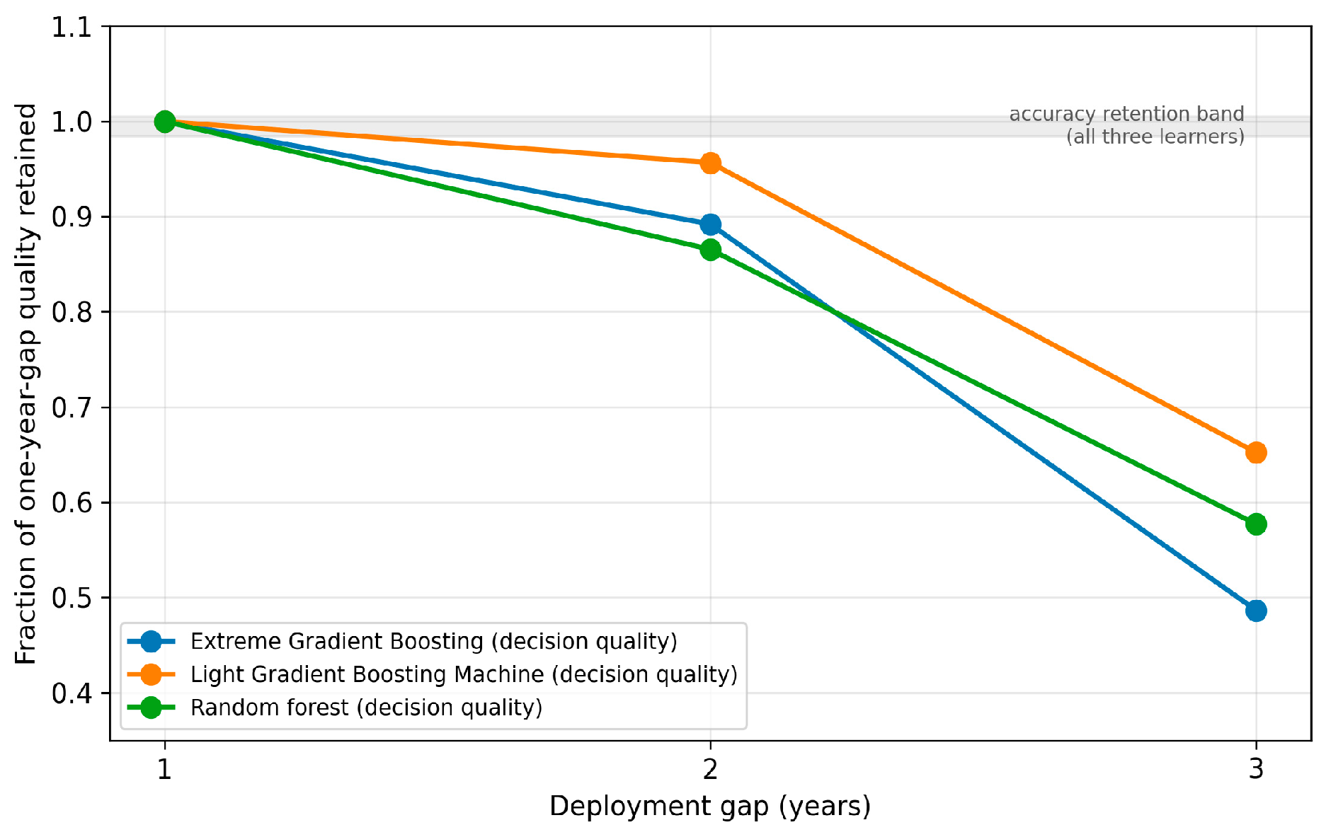
Table A1 reports, for each learner, the accuracy retained and the decision quality retained at a three-year deployment gap. The pattern is consistent across all three learners. Accuracy is essentially unchanged, with 98 to 101 percent of the one-year-gap AUC retained. Decision quality is not. Site-overlap retention at three years is 38 to 40 percent. The evaluation gap, the difference between accuracy retention and decision-quality retention, is 50 percentage points for Extreme Gradient Boosting, 35 for the Light Gradient Boosting Machine, and 41 for the random forest.
Table A1.
Accuracy retention and decision-quality retention at a three-year deployment gap, for three base learners. The pattern of near-stable accuracy and sharply decayed decision quality is consistent across learners.
Figure A1 plots the decision-quality decay curves for the three learners against the band of accuracy retention. All three decision curves fall far below the accuracy band, though they decay at somewhat different rates. The finding is therefore not an artefact of the gradient-boosting algorithm. The divergence between accuracy and decision decay comes from the structure of the evaluation problem, not from the learner. Aggregate accuracy is insensitive to reordering within the high-risk tail (Section 4.4), and this holds across both boosting and bagging ensembles.
Figure A1.
Decision-quality decay is consistent across base learners. Each curve shows the fraction of one-year-gap decision quality retained as the deployment gap increases, for Extreme Gradient Boosting (blue), the Light Gradient Boosting Machine (orange) and the random forest (green). The shaded band marks the range of accuracy retention across the three learners. The figure has a single panel and therefore carries no subfigure labels.
Appendix B. Which Features Drive the Instability: A Per-Year SHAP Analysis
Studies 1 to 3 show that the rankings produced by a crash-severity model decay with age. This appendix provides a descriptive companion. It asks which input features drive the instability. It examines how each feature’s contribution changes from year to year. The analysis is descriptive and exploratory. It is not a hypothesis test. It is reported to give insight into the source of the instability [17].
For each of the four study years, a separate model is trained. SHAP values are then computed for every crash in that year. Two summaries are extracted per feature per year. The first is the mean absolute SHAP value, which measures how much the feature contributes. The second is the sign of the correlation between the feature value and its SHAP value, which indicates the direction of the effect. Comparing these across years shows which features are stable and which are not.
Table A2 reports the year-to-year instability of feature contribution. It is measured as the coefficient of variation of the mean absolute SHAP value across the four years. Two patterns appear. The road-condition features are the most unstable. The side-fencing feature has a coefficient of variation of 73 percent, and the poor-surface feature 60 percent. Heavy-truck involvement is also unstable at 40 percent. By contrast, the features that contribute most on average, namely segment length, region, and number of lanes, are comparatively stable, between 15 and 18 percent. The instability is concentrated in a subset of features.
Table A2.
Year-to-year instability of feature contribution, 2017 to 2020, measured as the coefficient of variation of the mean absolute SHAP value. Road-condition features are the most unstable. The highest-contributing features are comparatively stable.
A second observation concerns direction. For most features, the direction of the effect is stable across the four years. Three features, however, reverse the sign of their SHAP direction at least once. These are month, time of day, and poor road surface. For these features, the model learned a different relationship in different years. Such reversals are a feature-level form of the temporal instability that the main studies detect at the level of decisions. Figure A2 displays both summaries.
Figure A2.
Per-year SHAP analysis. (a) Mean absolute SHAP value of the leading features across the four study years. (b) Year-to-year instability of feature importance, by coefficient of variation. The red bars mark features whose contribution varies by more than 40 percent across years and blue bars those that vary less, as indicated in the legend.
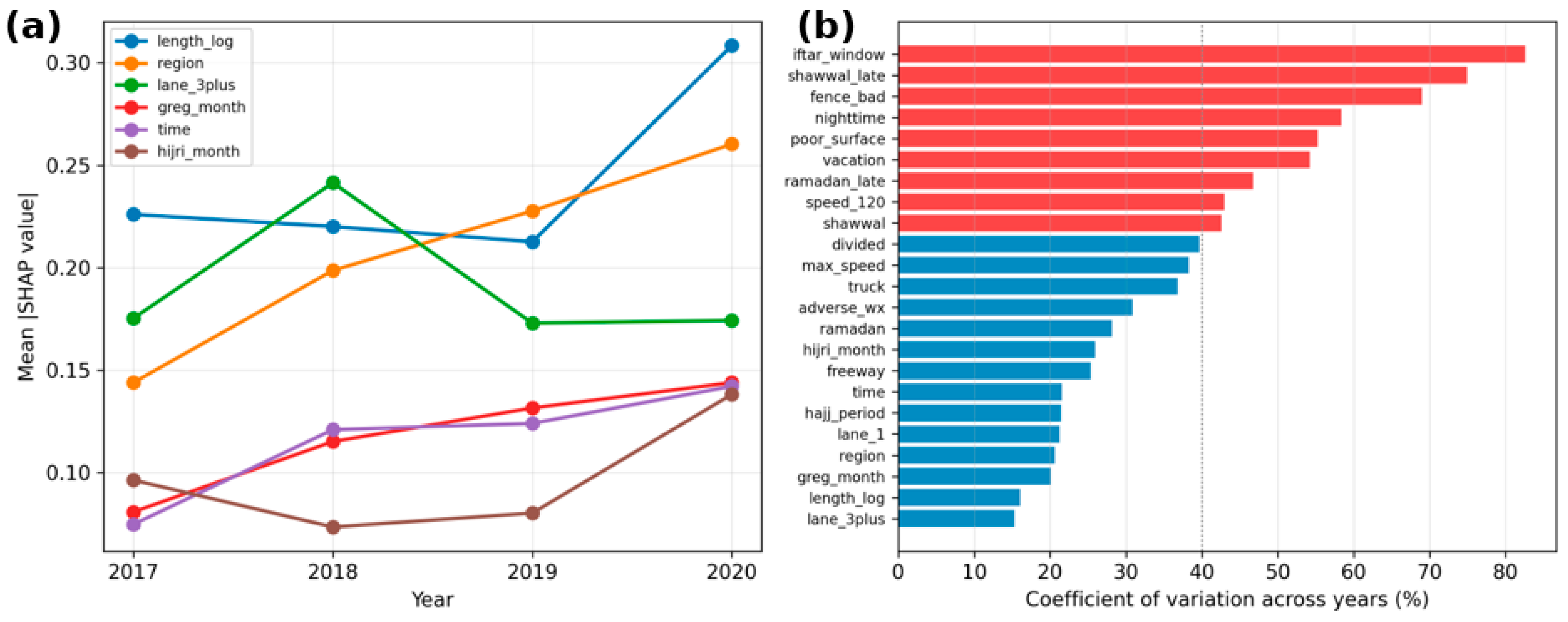
Two points about interpretation should be made. First, the analysis is descriptive. It characterises how the fitted models differ across years. It does not by itself establish why the process changed. The road-condition features that are most unstable are also among those most likely to be affected by recording variation in the road-inventory survey. Their apparent instability may reflect changes in recording as much as genuine changes in effect. The data do not allow the two to be separated. Second, the appearance of a temporal feature among those whose direction reverses is consistent with temporal instability. No specific calendar mechanism is inferred from it. The analysis is offered only as a descriptive map of where the instability is concentrated. That map is useful. It suggests that practitioners should watch the road-condition inputs, whose contribution is the least stable over time.
Appendix C. Robustness to the Definition of the Decision Unit
The primary analysis defines a site as the combination of administrative region, road type, posted-speed band, and time-of-day bin. Reviewers of this work reasonably asked whether the reported evaluation gap is a property of that particular aggregation. This appendix repeats the core forward-in-time analysis under five alternative definitions of the decision unit, spanning coarser and finer granularity, including a road-length-band definition that serves as the closest available proxy for a physical road segment. All other elements of the protocol are held identical.
Table A3 reports, for each definition, the number of panel sites, the top-20 percent overlap at the one-year (deployable baseline) and three-year gaps, and the resulting evaluation gap. Two conclusions follow, and we state both plainly.
Table A3.
Forward-in-time results under five alternative site definitions. Overlap at the one-year gap is the deployable baseline. The evaluation gap is accuracy retention minus decision-quality retention at the three-year gap.
First, for the two fine-grained definitions with substantial panels, the primary definition (291 sites) and the finest definition (458 sites), the evaluation gap is large and clearly present, at about 45 and 27 percentage points, respectively. Accuracy retention is approximately 98 percent in every definition, so the divergence between accuracy and decision quality is reproduced whenever the panel is large enough to support a meaningful ranking.
Second, and importantly, the three coarse definitions (33 to 77 sites) do not exhibit the gap, and their apparent decision retention exceeds 100 percent. We do not interpret this as evidence against the finding, and we caution against reading it as such. With so few sites, the three-year gap rests on a single training-test pair (2017 to 2020), and the top-20 percent list contains only seven to sixteen sites, so a single site changing position moves the overlap by six to fourteen percentage points. These estimates are dominated by sampling noise and cannot support a decay test. We report them for completeness rather than exclude them.
Taken together, the appendix supports a substantive conclusion that goes beyond robustness. The evaluation gap is not an artefact of one arbitrary aggregation, but it is a property of fine-grained decision units. Coarse strata aggregate many crashes per site, so their rankings are stable and decay little; fine strata, which is where operational screening actually targets treatment, aggregate fewer crashes per site, and decay substantially. Practitioners who target at fine granularity are therefore the most exposed to the risk this paper documents.
A limitation must be stated. The administrative extract supplied for this study contains no crash coordinates and no road-segment identifiers. Fixed-length segments, intersections, and grid cells therefore cannot be constructed from these data, and the road-length-band definition is the closest segment proxy available. Replication on geocoded crash records is a clear direction for future work.
References
- World Health Organization. Global Status Report on Road Safety 2023; World Health Organization: Geneva, Switzerland, 2023. [Google Scholar]
- Savolainen, P.T.; Mannering, F.L.; Lord, D.; Quddus, M.A. The statistical analysis of highway crash-injury severities: A review and assessment of methodological alternatives. Accid. Anal. Prev. 2011, 43, 1666–1676. [Google Scholar] [CrossRef] [Scilit] [PubMed]
- Mannering, F.L.; Bhat, C.R. Analytic methods in accident research: Methodological frontier and future directions. Anal. Methods Accid. Res. 2014, 1, 1–22. [Google Scholar] [CrossRef] [Scilit]
- Chen, T.; Guestrin, C. XGBoost: A scalable tree boosting system. In Proceedings of the 22nd ACM SIGKDD International Conference on Knowledge Discovery and Data Mining, San Francisco, CA, USA, 13–17 August 2016; pp. 785–794. [Google Scholar] [CrossRef] [Scilit]
- Wen, X.; Xie, Y.; Jiang, L.; Pu, Z.; Ge, T. Applications of machine learning methods in traffic crash severity modelling: Current status and future directions. Transp. Rev. 2021, 41, 855–879. [Google Scholar] [CrossRef] [Scilit]
- Seyfi, M.; Karimi Mamaghan, A.M.; Behnood, A.; Mannering, F. Analyzing crash injury severities with deep learning and advanced statistical models: An assessment of methodological challenges. Anal. Methods Accid. Res. 2025, 48, 100405. [Google Scholar] [CrossRef] [Scilit]
- Aldhari, I.; Almoshaogeh, M.; Jamal, A.; Alharbi, F.; Alinizzi, M.; Haider, H. Severity prediction of highway crashes in Saudi Arabia using machine learning techniques. Appl. Sci. 2023, 13, 233. [Google Scholar] [CrossRef] [Scilit]
- Alanazi, F.; Okail, M.A. Predicting traffic crash severity in Jeddah using machine learning techniques: A data-driven approach to road safety. Transp. Res. Rec. 2025, 2679, 324–343. [Google Scholar] [CrossRef] [Scilit]
- Liu, J.; Liu, W.; Li, X.; Chen, A.; Schonfeld, P.M.; Du, B. Hybrid ensemble learning model combining BERT and CNN for predicting urban rail transit accident consequences. IEEE Trans. Intell. Transp. Syst. 2025, 26, 12727–12739. [Google Scholar] [CrossRef] [Scilit]
- Ramspek, C.L.; Jager, K.J.; Dekker, F.W.; Zoccali, C.; van Diepen, M. External validation of prognostic models: What, why, how, when and where? Clin. Kidney J. 2021, 14, 49–58. [Google Scholar] [CrossRef] [Scilit] [PubMed]
- Mannering, F. Temporal instability and the analysis of highway accident data. Anal. Methods Accid. Res. 2018, 17, 1–13. [Google Scholar] [CrossRef] [Scilit]
- Behnood, A.; Mannering, F.L. The temporal stability of factors affecting driver-injury severities in single-vehicle crashes: Some empirical evidence. Anal. Methods Accid. Res. 2015, 8, 7–32. [Google Scholar] [CrossRef] [Scilit]
- Bayram, F.; Ahmed, B.S.; Kassler, A. From concept drift to model degradation: An overview on performance-aware drift detectors. Knowl. Based Syst. 2022, 245, 108632. [Google Scholar] [CrossRef] [Scilit]
- Hinder, F.; Vaquet, V.; Hammer, B. One or two things we know about concept drift: A survey on monitoring in evolving environments. Part A: Detecting concept drift. Front. Artif. Intell. 2024, 7, 1330257. [Google Scholar] [CrossRef] [Scilit] [PubMed]
- Montella, A. A comparative analysis of hotspot identification methods. Accid. Anal. Prev. 2010, 42, 571–581. [Google Scholar] [CrossRef] [Scilit] [PubMed]
- AASHTO. Highway Safety Manual, 1st ed.; American Association of State Highway and Transportation Officials: Washington, DC, USA, 2010. [Google Scholar]
- Mannering, F.L.; Shankar, V.; Bhat, C.R. Unobserved heterogeneity and the statistical analysis of highway accident data. Anal. Methods Accid. Res. 2016, 11, 1–16. [Google Scholar] [CrossRef] [Scilit]
- Niyogisubizo, J.; Liao, L.; Sun, X.; Adler, E.; Zhou, F.; Han, X.; Nziyumva, E. Predicting traffic crash severity using a hybrid of balanced bagging classification and light gradient boosting machine. Intell. Data Anal. 2023, 27, 79–101. [Google Scholar] [CrossRef] [Scilit]
- Lundberg, S.M.; Lee, S.I. A unified approach to interpreting model predictions. In Advances in Neural Information Processing Systems; Curran Associates: Red Hook, NY, USA, 2017; Volume 30, pp. 4765–4777. [Google Scholar]
- Qi, Z.; Yao, J.; Zou, X.; Pu, K.; Qin, W.; Li, W. Investigating factors influencing crash severity on mountainous two-lane roads: Machine learning versus statistical models. Sustainability 2024, 16, 7903. [Google Scholar] [CrossRef] [Scilit]
- Sorum, N.G.; Pal, D. Modeling driver injury severity using machine learning algorithms. Can. J. Civ. Eng. 2024, 51, 1302–1316. [Google Scholar] [CrossRef] [Scilit]
- Wu, Z.; Misra, A.; Bao, S. Modeling pedestrian injury severity: A case study of using extreme gradient boosting versus random forest in feature selection. Transp. Res. Rec. 2024, 2678, 1–11. [Google Scholar] [CrossRef] [Scilit]
- Jamal, A.; Umer, W. Exploring the injury severity risk factors in fatal crashes with neural network. Int. J. Environ. Res. Public Health 2020, 17, 7466. [Google Scholar] [CrossRef] [Scilit] [PubMed]
- Alanazi, F.; Umar, I.K.; Yosri, A.M.; Okail, M.A. Comparative evaluation of deep learning and traditional models for predicting traffic accident severity in Saudi Arabia. Sci. Rep. 2025, 15, 32568. [Google Scholar] [CrossRef] [Scilit] [PubMed]
- Malyshkina, N.V.; Mannering, F.L. Markov switching multinomial logit model: An application to accident-injury severities. Accid. Anal. Prev. 2009, 41, 829–838. [Google Scholar] [CrossRef] [Scilit] [PubMed]
- Behnood, A.; Mannering, F. Time-of-day variations and temporal instability of factors affecting injury severities in large-truck crashes. Anal. Methods Accid. Res. 2019, 23, 100102. [Google Scholar] [CrossRef] [Scilit]
- Alnawmasi, N.; Mannering, F. A statistical assessment of temporal instability in the factors determining motorcyclist injury severities. Anal. Methods Accid. Res. 2019, 22, 100090. [Google Scholar] [CrossRef] [Scilit]
- Alnawmasi, N.; Mannering, F. The impact of higher speed limits on the frequency and severity of freeway crashes: Accounting for temporal shifts and unobserved heterogeneity. Anal. Methods Accid. Res. 2022, 34, 100205. [Google Scholar] [CrossRef] [Scilit]
- Wang, L.; Huang, Y.; Li, Z. Temporal instability and unobserved heterogeneity of random parameters in single-vehicle crash severity analysis. Transp. Res. Interdiscip. Perspect. 2025, 34, 101721. [Google Scholar] [CrossRef] [Scilit]
- Hou, Q.; Huo, X.; Leng, J.; Mannering, F. A note on out-of-sample prediction, marginal effects computations, and temporal testing with random parameters crash-injury severity models. Anal. Methods Accid. Res. 2022, 33, 100191. [Google Scholar] [CrossRef] [Scilit]
- Agrahari, S.; Singh, A.K. Concept drift detection in data stream mining: A literature review. J. King Saud Univ. Comput. Inf. Sci. 2022, 34, 9523–9540. [Google Scholar] [CrossRef] [Scilit]
- Hovakimyan, G.; Bravo, J.M. Evolving strategies in machine learning: A systematic review of concept drift detection. Information 2024, 15, 786. [Google Scholar] [CrossRef] [Scilit]
- Yurdakul, B. Statistical Properties of Population Stability Index. Ph.D. Dissertation, Western Michigan University, Kalamazoo, MI, USA, 2018. [Google Scholar]
- Meyer, H.; Reudenbach, C.; Hengl, T.; Katurji, M.; Nauss, T. Improving performance of spatio-temporal machine learning models using forward feature selection and target-oriented validation. Environ. Model. Softw. 2018, 101, 1–9. [Google Scholar] [CrossRef] [Scilit]
- Stipancic, J.; Miranda-Moreno, L.; Saunier, N.; Labbe, A. Network screening for large urban road networks: Using GPS data and surrogate measures to model crash frequency and severity. Accid. Anal. Prev. 2019, 125, 290–301. [Google Scholar] [CrossRef] [Scilit] [PubMed]
- Bonera, M.; Barabino, B.; Yannis, G.; Maternini, G. Network-wide road crash risk screening: A new framework. Accid. Anal. Prev. 2024, 199, 107502. [Google Scholar] [CrossRef] [Scilit] [PubMed]
- Ghadi, M.; Torok, A. A comparative analysis of black spot identification methods and road accident segmentation methods. Accid. Anal. Prev. 2019, 128, 1–7. [Google Scholar] [CrossRef] [Scilit] [PubMed]
- Dhakal, B.; Al-Kaisy, A. Comparative analysis of the effectiveness of three proposed network screening methods for safety improvement sites on rural highways. Sustainability 2026, 18, 2008. [Google Scholar] [CrossRef] [Scilit]
- Kendall, M.G. A new measure of rank correlation. Biometrika 1938, 30, 81–93. [Google Scholar] [CrossRef] [Scilit]
- Aminghafouri, H.; Fu, L. Joint confidence region approach to ranking hotspot locations considering uncertainty in expected risk estimates. Transp. Res. Rec. 2024, 2678, 555–567. [Google Scholar] [CrossRef] [Scilit]
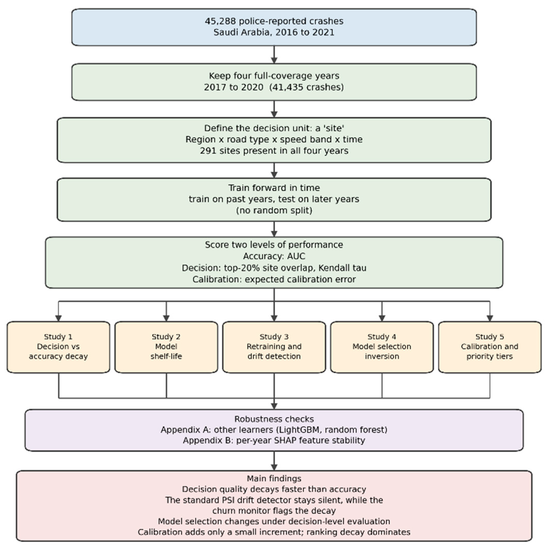
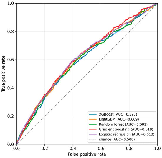
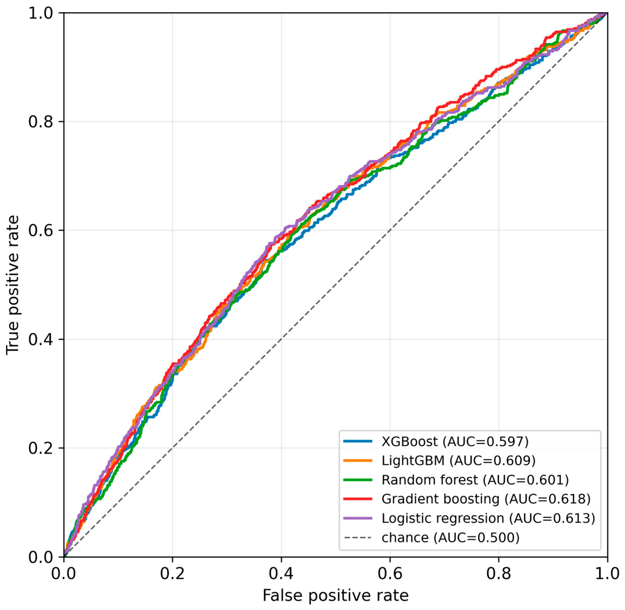
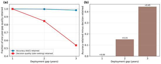
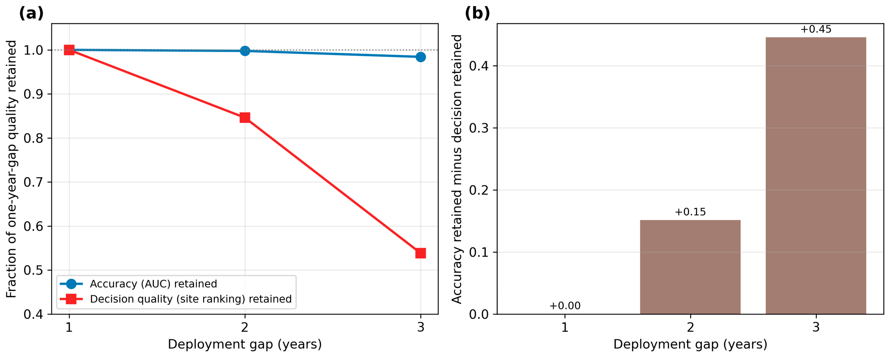
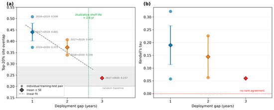
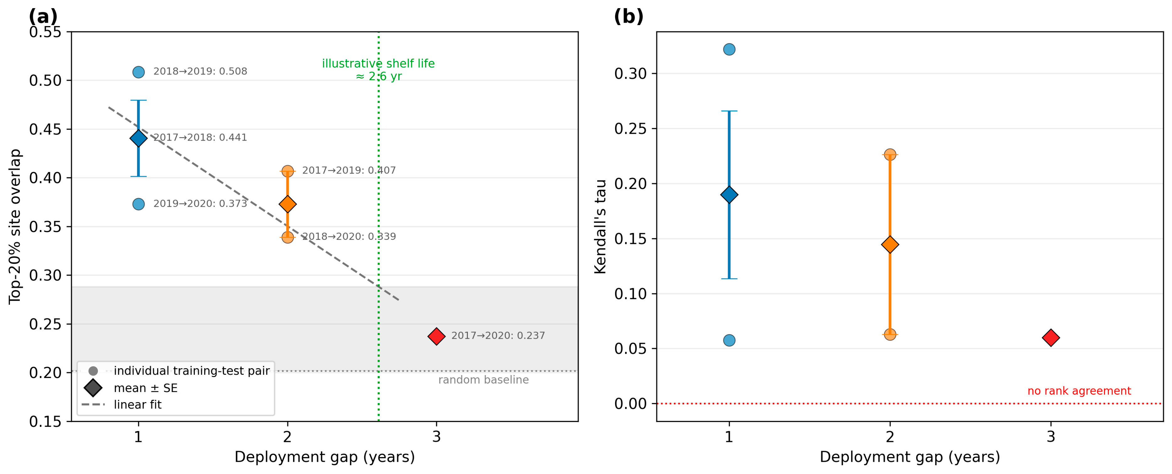
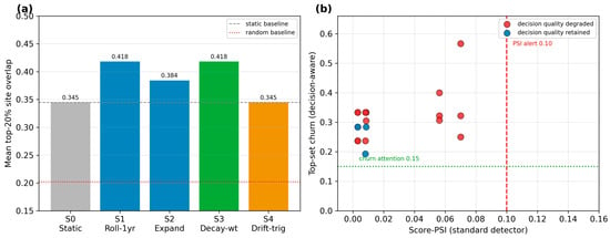
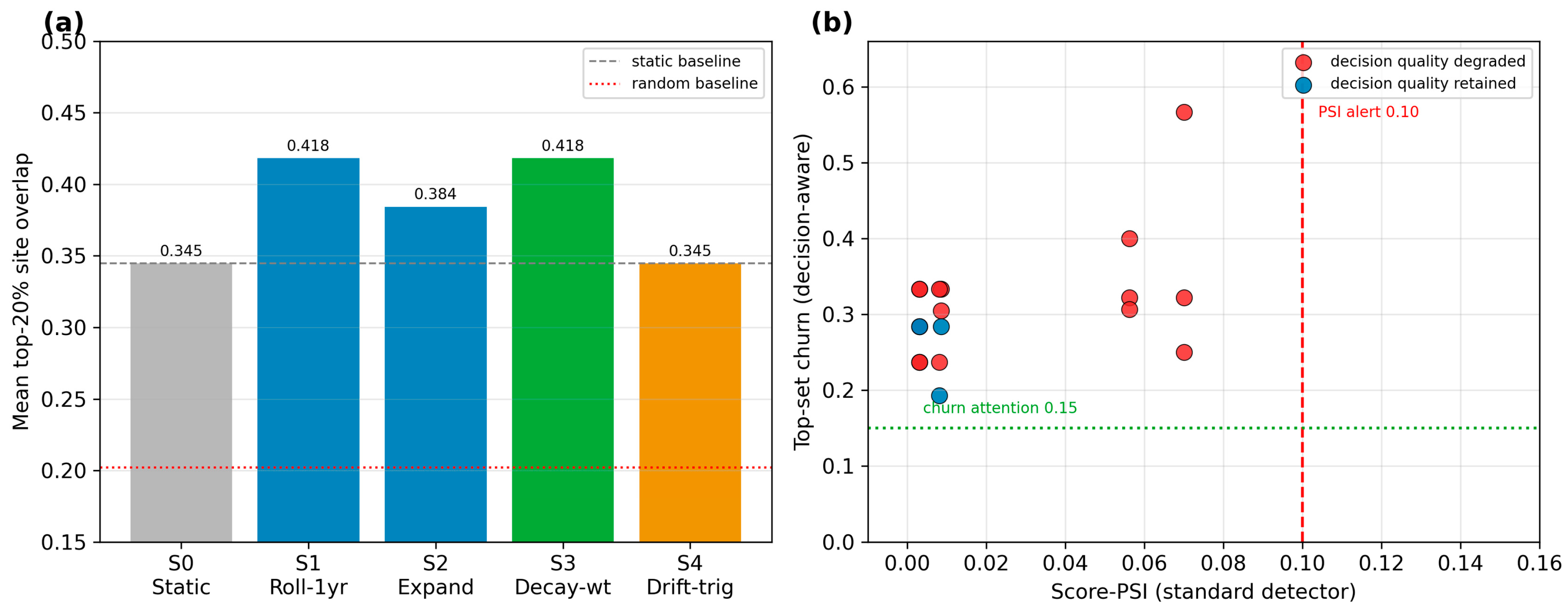
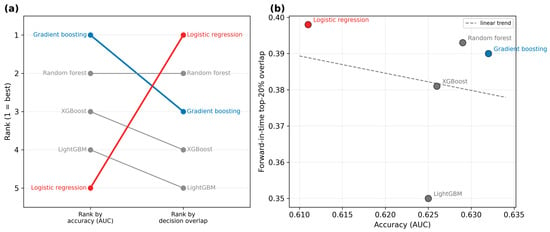
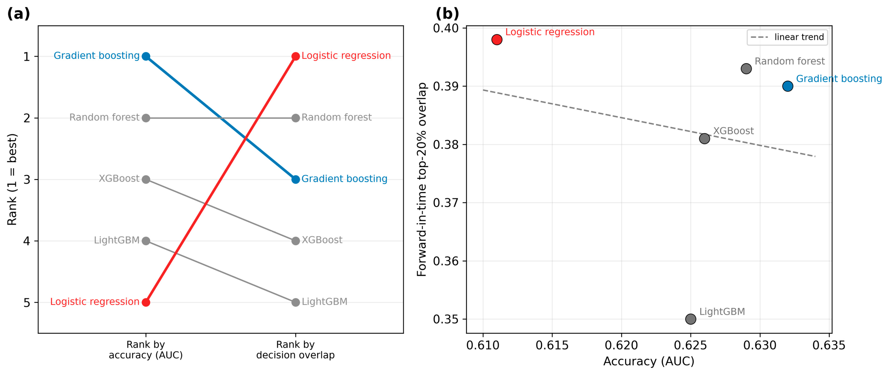

Disclaimer/Publisher’s Note: The statements, opinions and data contained in all publications are solely those of the individual author(s) and contributor(s) and not of MDPI and/or the editor(s). MDPI and/or the editor(s) disclaim responsibility for any injury to people or property resulting from any ideas, methods, instructions or products referred to in the content. |
© 2026 by the authors. Licensee MDPI, Basel, Switzerland. This article is an open access article distributed under the terms and conditions of the Creative Commons Attribution (CC BY) license.