


Abstract
Complexity matching helps explain how interacting physiological systems may become coordinated during shared experiences. In this study, we investigated group-level complexity matching by reconstructing heart rate variability (HRV) dynamics from 20 participants across six intervals of a guided heart-focused session. For each participant and interval, HRV was embedded in a two-dimensional delay-coordinate space using an interval-specific optimal delay. The reconstructed attractors were then analyzed using a Convolutional neural network (CNN) autoencoder, followed by clustering of the latent representations. The analysis identified three recurrent attractor morphology types: circular or loop-like attractors (Type 1), distorted circular attractors (Type 2), and distorted concentrated attractors (Type 3). In the complete sample of 20 participants (the primary analysis), Type 2 was more prevalent during the first three intervals, whereas Type 1 became more prevalent during the later intervals and was dominant in the final interval, increasing from 10.00% in Interval 1 to 60.00% in Interval 6 (Cochran’s Q(5) = 19.46, Holm-adjusted p = 0.0047). An exploratory secondary analysis restricted to the 15 participants whose morphology classification shifted across the protocol showed a similar pattern (increase from 6.67% to 66.67%; Q(5) = 20.00, Holm-adjusted p = 0.00375). This pattern suggests increasing similarity in HRV state-space organization, consistent with group-level complexity matching. The increase in Type 1 occurred during the later, more prosocially oriented intervals of this fixed-order protocol; because interval order was confounded with elapsed time and instruction repetition, this association should not be interpreted as a causal effect of the appreciation- or compassion-focused content. Coupled Thomas–Rössler systems further illustrated how nonlinear interaction can produce increasing similarity in attractor geometry. Compared with our earlier H-rank-based approach, the present method analyzes participant-specific reconstructed HRV attractor morphology using unsupervised CNN-autoencoder-based feature extraction and clustering. These findings suggest that attractor reconstruction and CNN-autoencoder-based clustering can reveal collective physiological organization that is not visually apparent in the raw HRV recordings. Whether conventional time-domain, frequency-domain, or entropy-based HRV indices would detect a comparable pattern was not directly tested here and remains an open question for future work.
1. Introduction
Synchronization is a fundamental principle that governs all the interactions across the natural world. From the coordinated migration of birds [1,2,3,4,5,6], which are guided by the Earth’s magnetic field, to the collective behaviors that are possibly observed in mammals [7,8,9,10], nature is filled with systems that operate in complete harmony. These interactions actually reveal the hidden patterns of synchrony as they demonstrate how the living systems exchange information and eventually align their internal dynamics with the very external cues. Likewise, humans are no exception. Human beings are also engaged in the subtle forms of physiological and psychological synchronization [11].
For example, during social interactions, whether between the doctor and patient [12,13,14,15], or members of a collaborating group, all the individuals naturally tune to one another [13]. From movements [14] to gestures [15], speech rhythms [16], and different kinds of emotional states [17], almost all, or some of those, begin to align during the synchronization phenomenon. Studies in the field of psychology, psychophysiology, and social neuroscience have shown that synchronized physiological activity often accompanies successful communication, empathy, and even group cohesion [18].
Consistent with this view, numerous studies indicate that coordinated behavior, especially when supported by shared visual cues, can enhance compassion and prosocial tendencies [16,17]. In social neuroscience, some studies have demonstrated that when individuals engage in a shared task, their neural rhythms may exhibit some temporal alignment, which indicates that similar perceptual and cognitive processes are being activated in parallel [18]. This phenomenon has been proposed as a basis for shared awareness or the subjective sense of “being together” [19,20]. Functional MRI research has revealed coupled temporal patterns between the speakers and the listeners during various communications [21,22,23,24,25]. Likewise, the analysis of EEG studies indicates that both verbal and nonverbal interaction can induce dynamic correspondences in the neural activity across individuals [26].
1.1. Related Work
Physiological synchronization during social interaction is frequently reflected in coordinated changes in complexity matching across individuals, which can be mathematically characterized through the analysis of complex biosignals such as the electrocardiogram (ECG) [12,27,28,29]. The ECG provides a direct measure of the heart’s electrical activity during successive cardiac cycles [30]. Thus, heart rate variability (HRV), which is derived from the ECG, actually quantifies the beat-to-beat fluctuations within the cardiac rhythm and therefore is defined as the time interval between consecutive R-wave peaks [31,32].
HRV is widely recognized as a marker of autonomic nervous system (ANS) health and activity. Numerous studies have shown that low levels of age-adjusted HRV are predictive of increased health risk and are associated with most chronic diseases and lower capacity for self-regulation [33,34].
HRV measures have been extensively employed for stress assessment and psychophysiological monitoring [35]. Many authors (including the HeartMath Institute and the broader HRV coherence literature) describe a coherent state as an HRV waveform that becomes more regular and sine-wave-like, often with spectral power concentrated near ~0.1 Hz; this pattern is more likely during calm, positive affect, whereas stress, anger, and anxiety are associated with more irregular, “incoherent” HRV patterns [36].
Because HRV signals are inherently nonlinear and nonstationary, their analysis requires analytical approaches that go beyond conventional summary statistics. A wide range of HRV analysis methods has been adopted in the research; to name a few, time-domain analysis methods, frequency-domain methods, and nonlinear approaches [37]. While time-domain measures (e.g., RMSSD) and frequency-domain methods provide useful global descriptors [38,39,40,41], they may fail to capture the adaptive, multiscale dynamics underlying synchronized physiological processes. Nonlinear HRV analysis methods, grounded in chaos theory and nonlinear dynamical systems, aim to characterize the complex and evolving structure of RR interval fluctuations [42,43,44,45,46].
Among nonlinear time-series analysis techniques, attractor reconstruction has emerged as a powerful framework for investigating complex physiological dynamics. By embedding time series data into a reconstructed state space, attractor-based methods characterize system behavior through geometric structure rather than isolated metrics. Multidimensional attractor reconstruction has been successfully applied to electroencephalography (EEG) signals, revealing changes in geometric complexity, differentiation across frequency bands, and causal asymmetries in neural interactions [47]. These findings support a process-oriented perspective in which integrative dynamics are shared across scales but may exhibit altered complexity under different physiological or cognitive conditions.
Similarly, nonlinear regulatory mechanisms govern cardiovascular dynamics, motivating the extension of attractor-based geometric analysis to ECG and HRV signals. Previous work has demonstrated that reconstructing ECG dynamics in state space can reveal distinctive geometric and chaotic characteristics associated with physiological conditions. For example, periodic split attractor reconstruction (PSAR) has been proposed to capture cycle-specific nonlinear dynamics of ECG signals [48]. When combined with deep learning architectures, such geometric representations have shown strong potential for distinguishing physiological states and detecting abnormalities. Related advances have also been reported for EEG, where deep learning–based state-space representations have been used to classify neural dynamics and identify pathological conditions such as epileptic seizures [49].
Cardiac dynamics therefore offer a promising physiological window for investigating interpersonal and group-level synchronization. Because HRV is noninvasive, easily accessible, and highly sensitive to autonomic regulation, synchronization of RR intervals has been repeatedly associated with positive features of social interaction, including cooperation, emotional attunement, and collective engagement. Empirical studies have reported HRV synchronization across coordinated activities such as rhythmic tapping, joint musical performance, singing, and therapeutic interactions, with nonlinear modeling approaches often outperforming linear methods in capturing coordination dynamics [50,51,52,53].
Despite the centrality of social and healing-oriented interactions to human experience, a key scientific challenge remains: can such interactions and the associated complexity matching phenomenon be objectively identified, quantified, and tracked at the level of physiological dynamics? Practices such as guided group meditation [11], heart-focused attention [29], and coherence-based exercises, including the approaches commonly described as Heart Lock-In [27] are widely used in therapeutic and group-coherence contexts. Although the participants frequently report subjective benefits such as emotional calming and enhanced interpersonal connection, but the mathematical evidence capturing these processes in real time remains limited.
1.2. The Present Study
In this study, we address this gap by analyzing HRV data collected during a guided group session with six consecutive experimental intervals. Each interval represented a different activity within a structured protocol. The protocol moved from individual focus to dyadic appreciation, group appreciation, global visualization, and compassion-focused imagery. We hypothesize that participants’ HRV reflects their physiological responses to the shared instructions and to their psychological engagement during the session. These responses can be represented as attractors reconstructed in a delay-coordinate state space. Therefore, our analysis does not focus mainly on the optimal delay values themselves. Instead, it focuses on the geometric organization and morphology of the reconstructed attractors as possible markers of complexity matching across participants.
Building on previous research on physiological coherence, HRV synchronization, and social coherence, this study offers a unique complexity-based perspective. Social coherence has been described as a harmonious alignment of relationships that supports effective communication and collective action. Earlier studies using multi-participant HRV monitoring have suggested that heart-focused practices, including Heart Lock-In techniques, may increase HRV coherence and physiological coordination within pairs and small groups. The present study extends this line of work by examining whether guided group coherence practices are associated with increasing similarity in the geometric organization of HRV dynamics, especially during intervals that emphasize appreciation, care, and compassion toward others.
This study builds on our earlier work characterizing complexity matching in a distant, non-contact healing protocol using the Hankel-rank (H-rank) algorithm [11]. In that study, group-level complexity matching between eight Healers and a single Healee was assessed by embedding a derived scalar complexity measure, the algebraic complexity (H-rank) of each participant’s RR-interval series, in a two-dimensional state space using a single time delay fixed across all nine phases of the protocol, with matching defined as statistical convergence of the mean H-rank of the Healer group toward that of the Healee. The present study differs from this prior work in several respects. First, attractors are reconstructed directly from the RR-interval (HRV) time series itself, rather than from a derived complexity index. Second, the embedding delay is optimized individually for each participant and each experimental interval, rather than fixed at a single value for the whole dataset. Third, complexity matching here is defined and assessed through categorical convergence in attractor shape: recurrent morphology types identified by an unsupervised CNN-autoencoder and K-means clustering procedure applied to the reconstructed attractor images of all participants individually, rather than through statistical convergence of a single scalar complexity index between a group average and one individual. Fourth, the present protocol involves 20 participants in symmetric roles undergoing a guided coherence and appreciation practice, in contrast to the asymmetric Healer–Healee roles and distant-healing intention protocol examined previously. Finally, the synthetic validation model used here to illustrate coupling-driven convergence, diffusively coupled Thomas cyclic and Rössler continuous-time chaotic systems, is distinct from the coupled logistic-map model used to validate the H-rank approach in [11].
The main methodological assumption of this study is that the changing dynamics of HRV can be represented by attractors reconstructed in a delay-coordinate state space. Attractor reconstruction was used to examine whether the geometric organization of each participant’s HRV dynamics changed across the six experimental intervals. Identical attractor shapes across participants were not expected, because HRV dynamics are naturally individual-specific. Instead, the study examined whether recurrent morphology types could be identified across the 20 participants and whether the distribution of these types changed as the protocol progressed. These morphology types provide a common way to compare individually different physiological dynamics and to examine possible convergence in HRV state-space organization at the group level.
Within this framework, attractor morphology is used as a shape-based descriptor of HRV state-space organization. We use the term complexity matching in the broader nonlinear-dynamics sense, in which interacting complex systems may exhibit increasing similarity in their complexity-related organization [54,55]. The analysis identified three recurrent morphology types: Type 1, a circular or loop-like attractor; Type 2, a distorted circular attractor; and Type 3, a distorted concentrated attractor. If more participants are assigned to the same morphology type during the same experimental intervals, we treat this as a group-level distributional pattern consistent with convergence in the broader framework of complexity matching. This aggregate measure does not, however, establish inter-individual physiological coupling and cannot distinguish mutual influence between participants from parallel convergence in response to shared external instructions. This interpretation therefore refers to convergence in the geometric organization of HRV dynamics, rather than exact point-by-point synchronization, identical physiological responses across individuals, or a demonstrated mechanism of inter-individual coupling. Representing cardiac dynamics through the shape of a reconstructed trajectory, independent of absolute amplitude, has a long precedent in cardiology. Vectorcardiography, introduced in the mid-20th century, displayed the heart’s electrical activity as a loop in a low-dimensional space and used the shape and orientation of this loop—rather than absolute lead voltage—as a basis for diagnostic interpretation [56]. The attractor-morphology approach used here extends this shape-based tradition to nonlinear, delay-coordinate reconstructions of HRV dynamics.
The study makes three main methodological contributions. First, interval-specific HRV attractors are reconstructed using an optimal time-delay embedding approach. Second, coupled synthetic nonlinear systems based on the Thomas cyclically symmetric and Rössler attractors are used to show how interaction between initially different dynamical systems can produce increasing similarity in attractor geometry. Third, a CNN-autoencoder-based framework is used to extract latent geometric features from attractor images and group them into recurrent morphology types. By combining nonlinear dynamical systems theory with machine-learning-based analysis, this study provides a quantitative framework for studying the individual HRV changes and group-level complexity matching during the guided coherence practices.
2. Materials and Methods
This section describes the experimental setup, participant characteristics, and data acquisition procedures, followed by the nonlinear time-series embedding approach used to reconstruct heart rate variability (HRV) attractors. Finally, a convolutional neural network (CNN)-autoencoder-based framework is introduced to extract geometric features from the reconstructed phase-space representations and to identify complexity matching patterns across participants.
Ethics Statement
This research was conducted in accordance with the Declaration of Helsinki and followed ethical guidelines for the protection of human participants. The analysis was approved by the Kaunas University Regional Ethics Committee for Biomedical Investigations (No. BE-1-30-2020). Informed consent was obtained from all participants. All personal identifiers were removed from the dataset prior to analysis, ensuring that individual participants could not be identified from the research findings. Strict confidentiality measures were maintained throughout the study.
Experimental Setup and Data Description
Heart rate variability data were collected from 20 adult participants, ranging in age from 31 to 75 years, including 7 females and 13 males. This sample is heterogeneous in both age and sex; potential effects of these factors on attractor morphology assignment were not modeled or statistically tested in the present study, for reasons explained in the Discussion (Limitations). The raw HRV recordings collected during the full experimental session are shown in Figure 1, where the x-axis represents time in seconds and the y-axis shows the RR interbeat interval recording. Participants were seated in a theater-style arrangement facing the front of the room. They were not informed of their individual performance during the session in order to minimize expectation effects and cognitive bias. Respiratory rate and breathing pattern were not monitored or experimentally controlled during the session.
Figure 1.
Raw RR-interval recordings for the 20 participants across the complete experimental session. Vertical dashed lines indicate the boundaries between the six experimental intervals. RR intervals are expressed in seconds.
HRV signals were recorded simultaneously from all participants using a custom-built data acquisition system consisting of 10 laptop computers connected via an Ethernet LAN. Each laptop was equipped with a two-channel photoplethysmography (PPG) module connected through a USB port. The modules were built around an 8-core Propeller microcontroller and enabled simultaneous PPG data collection from two participants. PPG signals were digitized at a sampling rate of 256 samples per second. An additional laptop served as the data server, receiving data from all acquisition computers over the LAN and storing the data locally.
PPG and HRV data processing was performed using DADiSP 6.5 (DSP Development Corporation, Newton, MA, USA). PPG signals used for heart rate variability (HRV) analysis were retrieved from the data acquisition server and detrended by subtracting a least-squares linear regression line. High-pass and low-pass Butterworth filters were used to remove low-frequency baseline drift below 1 Hz and high-frequency noise above 10 Hz. Following trend removal and filtering, a level-crossing function was used to identify the vertical center of the leading edge of each pulse waveform. Interbeat intervals (IBIs) were then obtained by calculating the time intervals between successive leading-edge centers.
Aberrant beats and artifacts were removed from the IBI records using a two-stage process. First, a computer algorithm eliminated intervals that varied by more than 30% from the mean of the previous four intervals. Any remaining artifacts were removed during second-stage editing, in which an experienced technician visually inspected the records. A regularly spaced time series was derived from the resulting series of normal intervals by linear interpolation of the irregularly spaced data, then resampled at 2 samples per second.
The full experimental session lasted approximately 26 min, corresponding to 1554 s. It consisted of six guided experimental intervals, each involving either an individual-focused or group-focused activity. All participants remained seated throughout the session and were exposed to identical instructions. For analytical purposes, the continuous HRV recordings were divided into six consecutive intervals, each corresponding to a distinct activity as shown in Figure 1. Interval boundaries were defined according to the onset and completion of each task within the HRV record.
Time Interval 1 (0–290 s; approximately 4.8 min) involved watching an inspirational video and served as the baseline condition. Time Interval 2 (293–470 s; approximately 3.0 min) consisted of a heart-focused breathing exercise emphasizing gratitude. Time Interval 3 (480–780 s; approximately 5.0 min) involved radiating appreciation toward the person seated next to the participant. In Time Interval 4 (789–1020 s; approximately 3.9 min), appreciation was expanded to the entire group. Time Interval 5 (1040–1310 s; approximately 4.5 min) focused on visualizing broader humanity, including world leaders, acting with care and dignity. Time Interval 6 (1330–1554 s; approximately 3.7 min) involved radiating unconditional love and compassion. Each participant was assigned a unique identification code as indicated along y-axis in Figure 1. The experimental protocol is summarized in Table 1.
Table 1.
Description of the experimental protocol.
Synthetic Nonlinear Systems: A Conceptual Illustration of Coupling-Induced Complexity Matching
To illustrate the concept of complexity matching, we first analyze synthetic data, numerically generated from the coupled nonlinear dynamical systems. Specifically, we use the Rössler and Thomas cyclically symmetric attractors as representative chaotic systems with distinct dynamics. By introducing bidirectional coupling between these systems, we demonstrate how interaction can cause their attractor geometries to become progressively more similar as the coupling coefficient increases, despite differences in the governing equations. This synthetic example provides an interpretive foundation for the subsequent analysis of HRV-derived attractors, where similar geometric convergence is hypothesized to reflect shared physiological and psychological engagement during the experimental protocol.
The Thomas cyclic and Rössler systems were chosen solely because they are two well-characterized and structurally distinct chaotic systems commonly used as generic testbeds in nonlinear dynamics. They are not proposed as mechanistic or mathematical models of cardiac autonomic regulation, and no attempt is made here to fit either system’s equations to the observed HRV data. Rather, the synthetic example is intended only to demonstrate, in a controlled and fully known setting, that coupling between two structurally distinct nonlinear systems can, in principle, produce convergence in reconstructed attractor geometry. It does not establish that the same coupling mechanism, or any particular coupling mechanism, underlies the patterns observed in the HRV data.
The Thomas cyclic symmetric attractor is a three-dimensional strange attractor originally proposed by René Thomas [57] and defined by the following system of coupled nonlinear ordinary differential equations:
where the parameter is set to to bring the system in the chaotic wandering mode. The Rössler system is formulated in three nonlinear ordinary differential equations originally proposed by Otto Rössler in year 1976 [58]:
where the parameters are set to , , and . We use diffusive coupling to couple the Thomas cyclic attractor to the Rössler attractor:
Note that the coupling terms are used to couple the systems across all three dimensions: with ; with ; with . All coupling terms vanish to zero when the two systems reach a fixed scaled (proportional) relationship as follows:
Rather than identical synchronization (x1 = x2, etc.). This scaled condition, rather than exact equality, reflects the intrinsically different amplitude ranges of the Thomas cyclic and Rössler attractors: the factor of 5 in the coupling terms compensates for this difference, so that proportionally matched trajectories, not equal-amplitude ones, drive the coupling term to zero. The first 5000 integration steps were discarded to remove transient behavior before visualizing the steady-state attractors. The resulting attractor geometries for different values of the coupling parameter ε are presented in Figure 2.
Figure 2.
Phase–space representations of the Thomas cyclic attractor and the Rössler attractor for increasing values of the coupling parameter . As increases, interaction between the systems leads to progressive changes in attractor geometry and increasing similarity, illustrating coupling-driven complexity matching.
The coupling parameter (epsilon) controls how strongly the Thomas cyclic system and the Rössler system interact, and it can be understood as the degree to which the two dynamical systems are allowed to “listen” to each other. When , the systems are completely independent, and no information is exchanged between them. When , the diffusive coupling is introduced, and information begins to flow between the systems. As increases, the mutual influence becomes stronger, promoting progressively greater similarity between the attractors. Importantly, even though the Thomas cyclic and Rössler attractors are generated by completely different differential equations and exhibit distinct intrinsic dynamics, diffusive coupling forces them to gradually adjust to one another, and this adjustment becomes visible as systematic changes in the attractor geometry. At , each attractor retains its characteristic structure (Thomas cyclic attractor appearing highly folded and irregular, and Rössler attractor maintaining its spiral-band form), reflecting the absence of interaction and therefore no complexity matching between the attractors. For small coupling values (e.g., ), the interaction acts as a weak constraint on the trajectories, reducing dispersion and initiating mild geometric synchronization, although the attractors remain clearly distinguishable because intrinsic dynamics still dominate. At intermediate coupling strengths (approximately ), the effect of interaction becomes pronounced, leading to substantial reconfiguration of both attractors: trajectories become smoother, chaotic wandering is reduced, and the global state-space structures become increasingly similar. This example provides a clear synthetic illustration of the complexity matching, where coordination is expressed not as point-by-point synchronization but as convergence in the overall geometric organization and effective similarity in terms of the complexity of the attractors. At larger coupling values (e.g., ), coupling dominates even more strongly, producing attractors that are markedly smoother and lower in apparent complexity, with both systems exhibiting highly aligned geometric structure. Overall, the progressive convergence of attractor geometry with increasing demonstrates in a controlled synthetic setting that interaction alone can drive complexity matching between distinct nonlinear systems, thereby motivating the interpretation that similar attractor shapes observed in HRV-derived reconstructions may reflect shared or coupled physiological dynamics during the experimental protocol.
Time-Series Embedding and Attractor Reconstruction
Let a scalar time series be given as . The technique used to represent time-series data in the form of vectors in a higher-dimensional space is known as time-series embedding. The space in which the reconstructed time series is represented is referred to as the time-delay coordinate space. Using this approach, the time series can be reconstructed into a set of dimensional vector points:
where where is the vector of time lags between successive measurements in the reconstructed phase space, and is the length of the time series. In general, time-series embedding depends on both the embedding dimension and the choice of time delays, which can be determined using various criteria depending on the complexity of the analyzed system. In this study, we adopt the geometrical approach for embedding time series into dimensional delay coordinate space, as presented in [59]. A discrete objective function was proposed to determine the optimal vector of time delays and is defined as:
where . The optimal vector of time delays is obtained by maximizing the objective function subject to the constraint where denotes the maximum allowable time lag.
For clarity and reproducibility, delay selection was performed by an exhaustive search over all integer delays in the range (), evaluating the objective function at each candidate value and selecting the delay that maximized it. This procedure was applied independently to each of the 120 participant–interval combinations (20 participants × 6 intervals).
In this study, the embedding dimension was fixed to for two reasons. First, each interval-specific HRV segment is relatively short (typically a few minutes), and standard techniques for validating a higher embedding dimension, such as false nearest neighbors, require longer and more stationary series to yield stable estimates; applying such techniques separately to each of the 120 short segments used here would not have produced reliable dimension estimates. Second, and more fundamentally, the two-dimensional embedding was chosen because the subsequent analysis explicitly compares attractor shape through two-dimensional images processed by a convolutional neural network (see below); was therefore a deliberate methodological choice tied to this image-based, shape-comparison approach, rather than an attempt to recover a topologically exhaustive reconstruction of a higher-dimensional physiological attractor. Consequently, the delay-coordinate reconstruction reduces to selecting a single optimal time delay for each signal segment, with . Because a poorly chosen delay can cause the reconstructed trajectory to collapse toward the diagonal of the embedding space—that is, excessively correlated coordinates that compress the apparent geometry of the attractor—the objective function described above was used to determine an interval-specific optimal time delay for each participant and each experimental interval individually, maximizing the spread of the reconstructed trajectory in the two-dimensional space for that specific segment. This per-attractor optimization, rather than the use of one fixed or arbitrarily chosen delay across the dataset, was intended specifically to minimize the risk of such collapse for the fixed embedding dimension used here. The optimization process itself is not visualized; instead, the resulting optimal delays were used to reconstruct the HRV attractors.
Why Optimal Time Delay Is Not Used as a State Descriptor
Although the optimal time delay contains information about the temporal structure of an HRV signal, it is not sufficient by itself to characterize the organization of the underlying dynamics during an experimental interval. In the present analysis, serves primarily as a reconstruction parameter that determines the temporal separation between coordinates in the delay-coordinate space. It is therefore used to construct the attractor rather than as a direct descriptor of physiological state.
Reducing a complex and nonstationary HRV signal to a single scalar value such as would discard much of the temporal and geometric information contained in the original time series. Participants or intervals with similar optimal delay values may still exhibit different state-space organizations, while different delay values may produce attractors with broadly comparable geometric characteristics. For this reason, the analysis focuses on the morphology of the reconstructed attractor rather than on the optimal delay value alone.
For each participant, attractor morphology was compared across the six experimental intervals to examine whether the geometric organization of the reconstructed HRV dynamics remained relatively stable or changed as the protocol progressed. The analysis also examined whether recurrent morphological patterns could be identified across participants, despite the expected inter-individual variability in HRV dynamics.
Changes in attractor morphology were interpreted as changes in HRV state-space organization within the present analytical framework. They were not used to determine the specific psychological, emotional, or physiological cause of those changes. Similarly, the absence of a morphological transition was not interpreted as evidence that no physiological or emotional response occurred.
CNN-Autoencoder-Based Feature Extraction and Attractor Morphology Clustering
To systematically compare the reconstructed attractors across participants and experimental intervals, each attractor was converted into a two-dimensional image and analyzed using a convolutional neural network autoencoder. This approach reduced the reliance on subjective visual inspection by learning numerical representations of the dominant geometric characteristics of the attractor images. Although the exact attractor shapes were not expected to be identical across participants, similarities in their learned morphological representations provided a basis for examining complexity matching.
Each reconstructed two-dimensional attractor, represented by the set of embedded coordinate pairs for a given participant and experimental interval, was rendered as a single continuous black trajectory line on a plain white background, without markers, grid lines, or axis labels, using the MATLAB R2025b Image Processing Toolbox. All 120 attractor images were generated using identical rendering settings, including a fixed image resolution of 104 × 104 pixels, a fixed line width of 0.5 pt, and the same color scheme. The fixed image dimensions ensured consistency with the encoder architecture shown in Figure 3, in which three successive 2 × 2 max-pooling operations reduced the spatial dimensions from 104 × 104 to 13 × 13, resulting in a 13 × 13 × 128 feature map before flattening. For each image, the x- and y-axis limits were set individually to the minimum and maximum values of that attractor’s reconstructed coordinates, with no additional margins, rather than to a single shared coordinate range across all participants and intervals. This per-image scaling was chosen because the purpose of the analysis was to characterize attractor morphology—that is, the shape and organization of the reconstructed trajectory—rather than the absolute physiological amplitude of the RR-interval fluctuations. Each attractor was therefore represented independently of its own dynamic range, consistent with the shape-based definition of attractor morphology described in Section 1 and Section 2.
Figure 3.
Training dynamics of the convolutional autoencoder with 3 convolutional blocks comprising 32, 64, and 128 filters, a latent layer of dimension 2048, and followed by the mirrored convolutional blocks. The best validation loss is 32.1260, 32.3831, and 32.5895 in parts (A, B, and C), respectively. Each result was obtained with a random 80/20 training and testing split.
The autoencoder consisted of an encoder and a decoder. The encoder transformed each attractor image into a lower-dimensional latent representation, whereas the decoder attempted to reconstruct the original image from this representation. During training, each attractor image was used as both the input and the reconstruction target. The network therefore learned its feature representation in an unsupervised manner, without requiring manually assigned morphology labels.
As illustrated in Figure 3, the encoder contained three two-dimensional convolutional layers. The first convolutional layer used 32 filters of size 3 × 3, the second used 64 filters of size 3 × 3, and the third used 128 filters of the same size. A rectified linear unit activation function was applied after each convolutional operation. Each convolutional layer was followed by 2 × 2 max-pooling, progressively reducing the spatial dimensions of the feature maps while retaining the principal geometric information contained in the attractor images.
After the third max-pooling operation, the resulting 13 × 13 × 128 feature representation was flattened into a vector containing 21,632 values. A fully connected layer then reduced this representation to a 2048-dimensional latent vector. This latent vector served as a numerical representation of the geometric characteristics of the corresponding attractor, including its global organization, trajectory concentration, deformation, and loop-like structure.
The decoder mirrored the dimensional transformation performed by the encoder. The 2048-dimensional latent vector was first projected through a fully connected layer to 21,632 values and subsequently reshaped into a 13 × 13 × 128 feature map. A sequence of convolutional and 2 × 2 upsampling layers was then used to restore the spatial dimensions of the image. ReLU activation functions were applied throughout the intermediate decoder layers, while a sigmoid activation function was used in the final convolutional layer to generate the reconstructed output image. The described architecture was chosen after testing different combinations and sizes of neural layers, considering layers with 32–128 convolutions of dimensions 2 × 2 or 3 × 3, pooling, upsampling, and dense layers with 1024–21,632 neurons.
Leave-one-out cross-validation for the training of the autoencoder was performed on the first data segment. During each run, one image was left out, and the remaining ones were split into training and testing samples: 19 and 4 images, respectively. Depending on the run, 12 to 50 epochs are required to finalize the training.
A small number of images also increases the risk of training falling into a local minimum, often that is the average image. Random initialization of neural weights adds to this challenge too. In order to avoid that, the final autoencoder architecture was trained several dozen times, and the result with the least visual difference between the input and the output images was selected as the final model. Three examples of the training dynamics of the optimal neural architecture are depicted in Figure 3. Validation loss is very similar between these three outputs, but the last one is selected for further analysis.
Side-by-side comparison of the input and the output HRV attractor images is provided in Figure 4. The blurring is visible and also expected since the bottleneck of the autoencoder compresses the information. Nevertheless, it is clearly seen that the output images preserve the overall morphology of the attractors as well as some of the more visible accents. This suggests that the information in the latent representations preserves the information on the relative attractor morphologies.
Figure 4.
Comparison between the input (left) and the output (right) HRV attractor images from the first segment using the optimal autoencoder architecture.
Training of the CNN-Autoencoder was performed as follows. Training/validation split was 80/20, with the Euclidean distance as the loss function and the stochastic gradient descent optimizer. After further number of trials, the number of epochs was set to 50, and the early stopping criterion was 10 epochs with no improvement in the loss. Batch size was set to 1 to use every input during each epoch. All other parameters were left as standard.
After training, the encoder was used to extract a 2048-dimensional latent feature vector from each reconstructed HRV attractor. PCA was then applied to the latent representations, and the first two principal components were retained as the feature space for K-means clustering. K-means clustering with K = 3 was therefore performed on the two-dimensional PCA representation, rather than directly on the original 2048-dimensional latent vectors. The purpose of the clustering procedure was to group attractors with similar learned geometric characteristics within each experimental interval and thereby identify recurrent morphology types that could be compared across intervals.
For the present exploratory analysis, K = 3 was selected to represent the three recurrent geometric configurations identified during preliminary examination of the reconstructed attractors. Accordingly, K-means clustering was performed with K = 3. The resulting clusters corresponded to Type 1, a circular or loop-like morphology; Type 2, a distorted circular morphology; and Type 3, a distorted concentrated morphology. These morphology assignments provided a common framework for comparing attractors that differed in their exact individual geometry but shared broader structural characteristics.
Principal component analysis was subsequently applied to the 2048-dimensional latent vectors to visualize their organization in a two-dimensional feature space. The first two principal components were used for graphical representation of the clustering results. Then, K-means assignments were determined from the two-dimensional PCA projection. Increasing the similarity in morphology assignments across participants during the same experimental intervals was interpreted as being consistent with complexity matching. The complete CNN-autoencoder architecture is presented in Figure 5.
Figure 5.
The layout of the convolutional neural network architecture used for autoencoding and clustering of HRV attractor images.
Statistical Analysis
Statistical analysis was performed to determine whether the distribution of attractor morphology types changed systematically across the six experimental intervals and whether the observed increase in a common morphology exceeded descriptive variation alone. This analysis was motivated by the central hypothesis of the study that, as the experimental protocol progressed, participants would show increasing similarity in the geometric organization of their reconstructed HRV attractors. Within the framework of the present study, such an increasing predominance of a common attractor morphology is interpreted as being consistent with group-level complexity matching. The statistical analysis therefore aimed to evaluate whether the observed redistribution of morphology types across the protocol was statistically supported rather than relying solely on descriptive changes in prevalence. Because the same participants were evaluated repeatedly throughout the protocol and morphology assignment represents a categorical outcome, the analysis was designed to account for the repeated-measures structure of the data. For each morphology type (Type 1, Type 2, and Type 3), the classification was represented as a binary outcome indicating the presence or absence of that morphology for each participant at each experimental interval. Cochran’s Q test was used to determine whether the prevalence of each morphology type differed significantly across the six repeated intervals [60]. Because separate Cochran’s Q tests were performed for the three morphology types, p values were adjusted for multiple testing using the Holm procedure [61].
To further examine differences between individual experimental intervals, exact McNemar tests [62] were used for pairwise comparisons. All possible pairs of the six intervals were evaluated separately for each morphology type, and the resulting p values were adjusted for multiple comparisons using the Holm procedure [61]. Particular attention was given to the comparison between Interval 1 and Interval 6 to characterize the change between the beginning and the end of the experimental protocol. To complement significance testing with an estimate of the magnitude and uncertainty of the observed change, the difference in morphology prevalence between Interval 1 and Interval 6 was additionally expressed as an absolute percentage-point change (Δpp). A 95% confidence interval for this paired prevalence difference was estimated using participant-level bootstrap resampling [63] with 10,000 iterations. Resampling was performed at the participant level to preserve the paired repeated-measures structure of the data. Statistical significance was evaluated at α = 0.05 using Holm-adjusted p values where applicable.
3. Results
Attractor reconstruction produced 120 state-space attractors, one for each of the 20 participants across the six experimental intervals. Comparing attractor morphology across intervals showed that the geometric organization of HRV dynamics was not static. For most participants, attractor morphology changed detectably as the protocol progressed. These comparisons identified observable morphological transitions, without assigning a specific psychological or physiological cause to any individual transition. Considerable inter-individual variability was observed among the 120 reconstructed attractors, and exact geometric agreement between participants was neither expected nor required. Because of space limitations, the complete set of individual attractor plots is not reproduced here. Instead, representative examples of the three morphology types are presented later in this section. After the state-space attractors were reconstructed, each attractor was converted into a two-dimensional image for further analysis. Visual inspection was useful for observing general geometric differences, but it was not sufficient for systematic grouping across all participants and intervals. Therefore, the attractor images were analyzed using a CNN-autoencoder-based clustering framework.
For each participant and experimental interval, the reconstructed attractor image was used as input to the CNN autoencoder. The encoder extracted geometric features describing the organization of each attractor and represented them as a 2048-dimensional latent feature vector. These latent vectors captured the main morphological characteristics of the attractor images in a form suitable for clustering and visualization.
The latent feature vectors were reduced to two dimensions using PCA and were then analyzed using K-means clustering with K = 3. This value was not selected by minimizing an internal cluster-validity index; rather, K = 3 reflects a specific, a priori hypothesis about attractor morphology, motivated by expert visual inspection of the reconstructed attractor images prior to any computational clustering. Primary visual examination of the representative attractors from multiple participants and intervals resulted in consistently identified three qualitatively distinct and recurring geometric forms: a closed, loop-like trajectory; a distorted but still recognizably circular trajectory; and a diffuse, concentrated trajectory without clear circular organization, corresponding directly to Type 1, Type 2, and Type 3 as used throughout this manuscript. The CNN-autoencoder-and-K-means pipeline described below was developed to formalize and automate this expert visual classification, rather than to conduct an unconstrained search for the numerically optimal number of clusters in the latent feature space. As a secondary, supporting check, we computed the Davies-Bouldin index for K = 2 to 10 (Figure 6B). The index decreases sharply between K = 2 and K = 3, then continues to decrease more gradually and with some non-monotonicity up to K = 10; lower Davies-Bouldin values are in fact observed for K = 5, 7, 8, and 10 than for K = 3. We do not interpret this as evidence that a larger K would give a more meaningful partition: like other internal cluster-validity indices, the Davies-Bouldin index has no mechanism for penalizing over-fragmentation and is not a reliable standalone indicator of the number of clusters corresponding to a data set’s true or theoretically meaningful structure, particularly in modestly sized samples. Taken to its logical extreme, minimizing this index would favor increasingly large K, up to the degenerate case of one cluster per observation, which would not constitute a meaningful morphology classification. We therefore treat the sharp initial improvement from K = 2 to K = 3 as broadly consistent with, but not independent statistical confirmation of, the three-category structure motivated above. The heuristic rule of thumb is reported for the same reason, as weak supplementary context rather than a rigorous justification on its own .
Figure 6.
Part (A) depicts a two-dimensional cluster plot for the 20 participants for the first experimental interval based on the first two principal components of the CNN latent representations. Davies-Bouldin index versus the number of clusters in the K-means classifier is shown in part (B).
K-means may give a different result depending on the initial choice of the centroids. For this reason, the clustering was repeated 10,000 times to test its stability; each run started at a random seed value. The results showed that there are 5 different clusterings. The case in Figure 6A is the second most probable clustering with a probability of 0.33. Despite that, it has the best (lowest) Davies-Bouldin index equal to 0.445 (compared to 0.459 for the most probable clustering having a probability of 0.47 and assigns P4, P5, and P10 to the class on the left). Note that the clustering was performed specifically on the first-time interval. The reasoning for such an approach is that the first interval acts as a fixed subset of data on which a single neural model is trained, and then the same model is used further in computing latent representations, followed by the per-interval clustering.
The resulting clusters corresponded to Type 1, the circular or loop-like morphology; Type 2, the distorted circular morphology; and Type 3, the distorted concentrated morphology. For visual presentation in the participant-by-interval morphology matrix, a consistent color-coding scheme was used: Type 1 was represented in green, Type 2 in blue, and Type 3 in yellow. These colors were used only as graphical labels for the morphology assignments. Principal component analysis was then applied to the latent feature vectors to visualize the cluster structure in a two-dimensional feature space. The first two principal components explained 68% of the total variance in the latent representations (PC1: 52%; PC2: 16%). Figure 6A shows the PCA projection of the CNN-autoencoder latent representations. Participants with similar latent geometric features are positioned closer together in the PCA projection, whereas participants with more distinct attractor characteristics appear farther apart. In Figure 6A, Participants P6 and P16 form a visibly separated group on the right side of the plot. Participants P2, P3, P7, P11, P17, P19, and P20 form another distinguishable group, while most of the remaining participants are located in the central region of the projection. These spatial patterns provide a visual summary of the differences and similarities among reconstructed attractor morphologies. It is important to note that the PCA projection was used for visualization as well as for the actual morphology assignments, which were obtained by applying K-means clustering.
At this stage, the morphology assignments obtained from the CNN-autoencoder-based clustering provided a complete overview of how the reconstructed HRV attractors changed across the six experimental intervals. These results are summarized in Figure 7 using a color-coded participant-by-interval matrix. In Figure 7, each row represents one experimental interval, each column represents one participant, and each cell shows the attractor morphology assigned to that participant during the corresponding interval. Type 1 is represented in green, Type 2 in blue, and Type 3 in yellow.
Figure 7.
Full participant-by-interval morphology matrix for all 20 participants. Arrows indicate P2, P9, P12, P13, and P16 as non-shifting. Type 1 morphology is represented in green, Type 2 in blue, and Type 3 in yellow.
Figure 7 also allows participants to be classified according to the stability of their morphology assignment across the protocol. Participants whose attractor was assigned to the same morphology type in at least five of the six intervals are classified as non-shifting; the remaining participants are classified as shifting. This is an operational, dataset-specific measure of classification stability that has not been independently validated; the label “non-shifting” describes only this stability and does not imply the presence, absence, or magnitude of any physiological or emotional response. Participants P2, P9, P12, P13, and P16 showed the least variation in attractor morphology across the six intervals and are classified as non-shifting under this criterion; the reason why these participants showed limited change in HRV state-space organization is beyond the scope of the present study. These participants are indicated by arrows in Figure 7. The complete sample of all 20 participants is retained for the primary statistical analysis reported below; the 15 shifting participants are additionally examined in a secondary, exploratory subgroup analysis, presented alongside the primary analysis in Table 2 and discussed further, including its limitations, in the Discussion. To illustrate the three morphology types more clearly, representative reconstructed HRV attractors from Interval 1 are shown in Figure 8. Figure 8 shows the attractors assigned to Type 1, the circular or loop-like morphology. During Interval 1, this morphology was observed for Participants P6 and P16. These attractors show a relatively organized loop-like structure compared with the other morphology types.
Table 2.
Morphology distribution and repeated-measures statistical analysis across the six experimental intervals: (A) complete sample (N = 20), primary analysis; (B) shifting subgroup (N = 15; excluding 5 non-shifting participants), exploratory secondary analysis.
Figure 8.
Reconstructed HRV attractors assigned to Type 1, the circular or loop-like morphology.
Figure 9 shows the attractors assigned to Type 2, the distorted circular morphology. During Interval 1, this morphology was observed for Participants P1, P4, P5, P8, P9, P10, P12, P13, P14, P15, and P18. These attractors retain a broadly circular or oval structure but show greater deformation and irregularity than Type 1.
Figure 9.
Reconstructed HRV attractors assigned to Type 2, the distorted circular morphology.
Figure 10 shows the attractors assigned to Type 3, the distorted concentrated morphology. During Interval 1, this morphology was observed for Participants P2, P3, P7, P11, P17, P19, and P20. These attractors show a more compact and densely concentrated trajectory pattern, with irregular excursions around a localized region of the reconstructed state space.
Figure 10.
Reconstructed HRV attractors assigned to Type 3, the distorted concentrated morphology.
As a secondary, exploratory view of the data, the morphology assignments of the 15 shifting participants (after excluding the five non-shifting participants) are shown separately in Figure 11. This figure provides a clearer view of how attractor morphology changed across the protocol among the subgroup of participants whose classification was not stable across intervals; the corresponding primary analysis of the complete sample of all 20 participants is presented in Table 2A below. In Figure 11, each row represents one experimental interval, and each column represents one shifting participant. The colors indicate the morphology assigned to each participant during each interval: Type 1 is shown in green, Type 2 in blue, and Type 3 in yellow. The shifting subgroup included Participants P1, P3, P4, P5, P6, P7, P8, P10, P11, P14, P15, P17, P18, P19, and P20.
Figure 11.
CNN classification results for the exploratory shifting subgroup, after excluding non-shifting participants. Type 1 morphology is represented in green, Type 2 in blue, and Type 3 in yellow.
Within this exploratory subgroup, the early intervals were dominated mainly by Type 2 and Type 3 morphologies, indicating that these participants did not begin the protocol with a single shared attractor pattern. Instead, their HRV dynamics showed considerable variation during the first part of the session. As the protocol progressed, however, the distribution of morphology types changed. In the later intervals, especially Interval 6, a larger number of participants were assigned to Type 1, the circular or loop-like morphology. This shift suggests increasing similarity in HRV state-space organization among the shifting subgroup during the later stages of the protocol; the corresponding pattern in the complete sample, which forms the primary evidence for this study’s conclusions, is reported in the next subsection. However, the figure should not be interpreted as showing identical HRV signals across participants. Rather, it shows convergence in the broader geometric organization of their reconstructed HRV attractors.
The distribution of morphology types across the six experimental intervals was analyzed statistically at two levels. The primary analysis used the complete sample of all 20 participants, avoiding any dependence on the shifting/non-shifting classification. Because the shifting subgroup is selected specifically on the basis that morphology classification changed across the protocol, restricting the analysis to this subgroup is structurally expected to accentuate the apparent temporal pattern; a second, exploratory analysis was therefore additionally performed on the 15-participant shifting subgroup, after excluding the five non-shifting participants. Both analyses are presented in Table 2, with the complete-sample primary analysis presented first as Table 2A and the exploratory subgroup analysis presented second as Table 2B.
The repeated-measures analysis confirmed that the prevalence of Type 1 changed significantly across the six experimental intervals in the complete sample (Cochran’s Q(5) = 19.46, p = 0.0016, Holm-adjusted p = 0.0047). Type 2 also showed a significant change across intervals (Q(5) = 12.94, p = 0.0239, Holm-adjusted p = 0.0478). In contrast, the distribution of Type 3 did not change significantly across the protocol (Q(5) = 5.92, p = 0.3142). Thus, although Type 3 decreased from 30.00% in Interval 5 to 15.00% in Interval 6, this fluctuation was not statistically supported as a systematic interval-related change. A direct comparison between the first and final intervals was additionally performed using McNemar’s test. For Type 1, prevalence increased from 10% in Interval 1 to 60% in Interval 6, corresponding to an absolute increase of 50.0 percentage points (95% bootstrap CI30 to 70). The direct Interval 1 vs. Interval 6 comparison was also statistically significant in the exact McNemar test (p = 0.0020) and remained significant after Holm correction (adjusted p = 0.0293). Both the overall repeated-measures test and the direct endpoint comparison therefore support a statistically robust redistribution toward Type 1 morphology across the protocol in the complete sample, independent of the shifting/non-shifting classification. Because the criterion used to define the shifting subgroup selects participants specifically on the basis that their morphology classification changed across the protocol, restricting the analysis to this subgroup is expected, by construction, to yield an equal or stronger apparent temporal pattern; we therefore report this subgroup analysis as exploratory rather than as independent confirmation. Table 2B presents the same analysis restricted to the 15-participant shifting subgroup, after excluding the five non-shifting participants. Within this exploratory subgroup, Type 1 prevalence increased from 6.67% in Interval 1 to 66.67% in Interval 6 (Cochran’s Q(5) = 20.00, Holm-adjusted p = 0.00375); the direct Interval 1 vs. Interval 6 comparison was significant before correction (p = 0.00391) but did not remain significant after Holm adjustment (adjusted p = 0.0586). We treat the complete-sample analysis (Table 2A) as the primary evidence for a statistically robust temporal redistribution toward Type 1 morphology, and the shifting-subgroup analysis (Table 2B) as a descriptive, exploratory supplement that should not be read as an independent replication, given that its selection criterion structurally favors detecting a pattern. Figure 12 illustrates the evolution of the three morphology types across the six experimental intervals for both the complete sample and the exploratory shifting subgroup. In both analyses, the later intervals are characterized by an increased prevalence of Type 1 and a corresponding reduction in Type 2, demonstrating a consistent redistribution of attractor morphology across the protocol. To assess whether the increasing prevalence of Type 1 could simply reflect interval duration rather than interval content, we compared the duration of each interval with the corresponding Type 1 prevalence in the complete sample (Table 2A) across the six intervals. Interval durations ranged from 177 s (Interval 2) to 300 s (Interval 3) and did not increase monotonically across the protocol; the final interval (Interval 6), which showed the highest Type 1 prevalence (60%), was one of the shorter intervals (224 s), whereas the longest interval (Interval 3, 300 s) showed one of the lowest Type 1 prevalences (15%). Across the six interval-level pairs, duration was not positively associated with Type 1 prevalence (Pearson r = −0.36, p = 0.49; Spearman ρ = −0.62, p = 0.19). Given the small number of intervals, this analysis is not statistically powered to confirm or exclude a duration effect and should therefore be interpreted as a descriptive check rather than a definitive test. It does not, however, support the hypothesis that the increasing prevalence of Type 1 during the later intervals is simply an artifact of longer interval duration.
Figure 12.
Distribution of attractor morphology types across the six experimental intervals. (A) Complete sample including all 20 participants—the primary analysis. (B) Shifting subgroup including 15 participants after excluding the five non-shifting participants—a descriptive, exploratory supplement (see Section 4). In both analyses, Type 1 is more prevalent during the later intervals, whereas Type 2 generally decreases. Because the subgroup shown in panel (B) is selected specifically on the basis that morphology classification changed across the protocol, panel (B) is structurally expected to show an equal or stronger apparent temporal pattern than panel (A) and should not be read as an independent replication of it.
4. Discussion
This study examined group-level complexity matching by looking at the geometric organization of reconstructed HRV attractors. Rather than characterizing the recordings using conventional summary HRV indices, the analysis treated HRV as a nonlinear physiological signal and focused on how its reconstructed state-space morphology changed across participants and experimental intervals. This approach allowed us to study similarity in the broader organization of HRV dynamics, rather than only looking for direct beat-to-beat synchronization between participants. The CNN-autoencoder-based clustering analysis identified three recurrent attractor morphologies across the dataset. These were Type 1, the circular or loop-like morphology; Type 2, the distorted circular morphology; and Type 3, the distorted concentrated morphology. The distribution of these morphology types changed across the six intervals. Among the shifting participants, Type 2 was the most common morphology during the first three intervals. However, its prevalence decreased during the later intervals. In contrast, Type 1 was less common at the beginning of the protocol but became more frequent in the later intervals and was dominant in Interval 6. The repeated-measures analysis confirmed that Type 1 prevalence changed significantly across the six experimental intervals (Cochran’s Q(5) = 20.00, Holm-adjusted p = 0.00375). Type 2 also showed a significant overall change, whereas Type 3 did not. Thus, the observed redistribution of morphology types was statistically supported and was not based on descriptive percentages alone. This shift toward Type 1 is the main result of the study. By the final interval, most shifting participants were assigned to the same broad attractor morphology, suggesting that their HRV dynamics became more similar in terms of state-space organization as the protocol progressed. Within the framework of this study, this increasing agreement in attractor morphology is interpreted as being consistent with group-level complexity matching, though, as discussed below, the fixed-order design means this pattern cannot yet be dissociated from time-on-task or repetition effects.
It is important to clarify what this result means. The finding does not mean that the participants’ HRV signals became identical, nor does it mean that they were synchronized point by point in time. Rather, it suggests that the overall geometric organization of their reconstructed HRV dynamics became more similar. In this sense, complexity matching is understood as convergence in nonlinear state-space structure, not as exact temporal synchronization. The timing of this pattern is also notable, though it must be interpreted cautiously. Type 1 became more common during the later intervals, which coincided with group-directed appreciation, broader care, and compassion-focused imagery. However, because the protocol followed a fixed, non-randomized order with no control condition, interval identity is fully confounded with elapsed time and with repetition of structurally similar instructions across six successive intervals. Consequently, the observed increase in Type 1 prevalence cannot be attributed to the appreciation- or compassion-focused content of the later intervals as distinct from simple time-on-task effects (e.g., progressive relaxation, fatigue, or postural adaptation over the session) or a repetition effect from receiving similar guidance repeatedly. The present design cannot separate these explanations, and the association reported here should be read strictly as descriptive rather than as evidence that the prosocial content of the later intervals drove the change.
The results are broadly consistent with previous work suggesting that heart-focused and positive emotional states may be linked with more organized HRV patterns and interpersonal physiological coordination. The present study extends this idea by showing that similarity may also appear at the level of reconstructed attractor morphology. In other words, participants may show comparable modes of nonlinear HRV organization even when their individual HRV time series remain different. From a methodological point of view, the study shows the usefulness of combining attractor reconstruction with CNN-autoencoder-based clustering. Attractor reconstruction made it possible to visualize the geometric organization of HRV dynamics: no clear cross-participant pattern is apparent to the eye in the raw RR-interval recordings alone (Figure 1), whereas the reconstructed attractors, once compared through the CNN-autoencoder, revealed recurrent morphology types and a shift in their distribution across intervals. We did not test whether conventional time-domain, frequency-domain, or nonlinear HRV indices computed on the same recordings would reveal a similar shift; this comparison is identified as a limitation below. The CNN autoencoder transformed the attractor images into 2048-dimensional latent feature vectors, which were reduced to two dimensions using PCA; this two-dimensional PCA representation was used both for K-means clustering and for visualization, providing a systematic way to group similar attractor morphologies.
The synthetic Thomas–Rössler example also supported the interpretation of the physiological findings. It showed that two different nonlinear systems can become more similar in attractor geometry when interaction is introduced. This provides a useful conceptual model for understanding how complexity matching may appear as geometric convergence between nonlinear systems. However, the synthetic example should not be interpreted as proof that the same coupling mechanism occurred in the HRV data. It is used only as a conceptual illustration of how interaction can produce similarity in state-space structure.
Some of the limitations should be noted. First, the sample size was modest (20 participants) and heterogeneous in age (31–75 years) and sex (7 women, 13 men). Potential effects of age and sex on attractor morphology assignment were not modeled or statistically tested here: with three morphology types distributed across 20 participants and six intervals, the resulting subgroups are too small to support a reliable covariate-adjusted or subgroup analysis, and a formal statistical test under these conditions would be more likely to produce an unstable or spurious result than a genuine one. We therefore report this as an open limitation rather than an analyzed factor. The participants also came from a specific experimental setting. Future studies with larger and more diverse samples should explicitly test for age- and sex-related effects on attractor morphology and complexity matching, with sufficient participants per subgroup to support adequately powered comparisons.
Second, as described in the Results, participants were classified as non-shifting when their attractor morphology remained in the same category for at least five of the six intervals; this criterion has not been independently validated and was applied post hoc to the present dataset. Because the exploratory subgroup analysis restricts the sample to participants classified as shifting—participants selected specifically because their morphology classification changed across the protocol—this subgroup is structurally expected to show an equal or stronger apparent temporal pattern than the complete sample, independent of any underlying effect. For this reason, we treat the complete-sample analysis (N = 20) as the primary analysis throughout the manuscript, and the shifting-subgroup analysis (N = 15) as a descriptive, exploratory supplement rather than independent confirmation. The term “non-shifting” describes only the stability of a participant’s morphology classification across intervals and does not imply that these participants showed no physiological or emotional response. Reassuringly, the complete-sample analysis—which does not depend on this exclusion criterion at all—itself showed a statistically significant redistribution toward Type 1 morphology across the six intervals (Cochran’s Q(5) = 19.46, Holm-adjusted p = 0.0047), including a significant direct Interval 1 versus Interval 6 comparison (Holm-adjusted p = 0.0293); indeed, this direct comparison was more robust in the complete sample than in the exploratory subgroup, where it did not survive correction (Holm-adjusted p = 0.0586). The shifting/non-shifting classification criterion nonetheless remains specific to the present dataset and should be validated in larger, independent samples before being used to define subgroups in future work. Third, several aspects of the CNN-autoencoder-based clustering procedure require further validation. In particular, because each attractor image was axis-scaled individually to its own coordinate range rather than to a shared range across participants and intervals, the resulting images emphasize trajectory shape independently of absolute physiological amplitude. Although this is consistent with our focus on attractor morphology, a small number of extreme reconstructed values, including those potentially arising from residual uncorrected recording artifacts, could disproportionately expand an image’s axis range and alter the apparent concentration of the trajectory, particularly for the Type 3 (distorted concentrated) category. Moreover, we did not systematically compare artifact-correction rates across participants and experimental intervals and therefore cannot fully exclude the possibility that residual artifacts were unevenly distributed or preferentially associated with particular morphology types. As a partial mitigating factor, all six experimental intervals were conducted with participants seated throughout the session (Table 1), reducing the likelihood of systematic differences in motion-related artifacts caused by changes in posture or activity.
A further limitation of the morphology-based approach is that discretizing the latent representations into three broad attractor types necessarily reduces continuous information and may obscure within-type variability. Pairwise distances between latent representations could provide a complementary continuous measure of similarity between participants. However, because the autoencoder used in the present study was trained for representation learning rather than metric learning, distances in the latent space were not explicitly constrained or validated to correspond to similarity in HRV attractor geometry. Future work should therefore investigate validated latent-space or attractor-distance measures alongside morphology prevalence to determine whether convergence occurs not only across broad morphology classes but also continuously within individual morphology types.
Relatedly, the identified morphology types were not directly compared with conventional HRV indices computed from the same data. In particular, time-domain measures such as SDNN and RMSSD, frequency-domain measures such as the LF/HF ratio, and nonlinear measures such as sample entropy were not evaluated alongside the attractor-based classifications. Consequently, the suggestion that attractor-morphology analysis reveals organization not readily apparent using conventional HRV analysis should be interpreted cautiously; in the present study, this observation is based on the absence of clear cross-participant convergence in the raw RR-interval recordings (Figure 1), rather than on a direct comparison with standard HRV metrics. Future studies should therefore compare different clustering algorithms, examine the sensitivity of morphology assignments to per-image versus shared axis scaling and to robust versus min–max-based axis limits, quantify artifact-correction rates by participant and interval, and test whether they are associated with morphology-type assignment, directly compare the identified morphology types with established time-domain, frequency-domain, and nonlinear HRV measures computed from the same recordings, and evaluate whether the same morphology types can be reproduced in independent datasets.
Fourth, the preprocessing procedure introduces an additional limitation related to the interpolation and resampling of the interbeat-interval series. Although the underlying PPG signals were acquired at 256 samples per second, the resulting irregularly spaced IBI series was linearly interpolated and resampled at 2 Hz prior to attractor reconstruction. A higher interpolation rate, such as 4 Hz, could potentially preserve additional fine-scale temporal structure and thereby influence the reconstructed attractor geometry. We did not formally test the sensitivity of the attractor morphology or the subsequent CNN-based classification to the choice of interpolation rate. Future work should therefore repeat the reconstruction and classification pipeline using alternative interpolation rates, for example 4 Hz, on the same or an independent dataset to determine whether the identified morphology types are robust to this preprocessing choice.
An additional limitation concerns the number of clusters, K = 3, used in the K-means step. This value was chosen a priori, based on expert visual identification of three recurring attractor morphologies, rather than by minimizing an internal cluster-validity index; indeed, the Davies-Bouldin index continued to decrease for several values of K larger than 3 (Figure 6B), a pattern consistent with the well-documented tendency of such indices to favor increasingly fine-grained partitions rather than evidence that these larger K values correspond to a more physiologically meaningful morphology taxonomy [64]. We did not systematically evaluate whether values of K other than 3 correspond to interpretable or reproducible morphology categories. Independent validation of the three-type taxonomy—for example, via blinded classification by additional expert raters, inter-rater agreement analysis, or a structured comparison of cluster interpretability across candidate values of K—is an important direction for future work.
A related methodological limitation is that the fixed embedding dimension (m = 2) was not validated using standard dimension-selection techniques such as false nearest neighbors or correlation-dimension saturation analysis. As explained above, this reflects both the short duration of the interval-specific HRV segments, which limits the reliability of such techniques, and the deliberate choice to represent each attractor as a two-dimensional image for shape-based CNN comparison. The time-delay optimization procedure used here was designed to minimize collapse of the reconstructed trajectory for this fixed two-dimensional embedding, but it does not establish that a two-dimensional embedding preserves the full topological structure of the underlying physiological dynamics. Future studies using longer or pooled HRV recordings should apply formal dimension-validation techniques to determine whether higher-dimensional embeddings reveal additional structure not captured by the two-dimensional representation used here.
Finally, and most importantly, the protocol used a fixed, non-randomized sequence of intervals with no control condition. This design does not allow the greater prevalence of Type 1 morphology during the later intervals to be attributed specifically to the gratitude- and compassion-focused content of those intervals. Because interval order and elapsed time are fully confounded, the observed pattern could also reflect time-on-task effects, including progressive relaxation, fatigue, or postural adaptation, repetition of structurally similar instructions across successive intervals, or physiological responses to the appreciation- and compassion-focused content itself. Respiration was not monitored or experimentally controlled, introducing an additional mechanistic uncertainty. Because the protocol included heart-focused breathing instructions, convergence toward similar breathing patterns across participants may have contributed to the observed redistribution toward Type 1 morphology. Respiratory sinus arrhythmia was retained as a physiological component of HRV rather than treated as an artifact during preprocessing. Consequently, the present data cannot distinguish respiration-related entrainment from the proposed group-level complexity-matching interpretation. Future studies should include simultaneous respiratory monitoring and, ideally, experimental control or adjustment for breathing rate to determine the extent to which respiratory synchronization contributes to the observed morphology patterns.
The present data cannot distinguish among these explanations, and a time-matched neutral or repeated-instruction control condition, together with randomized or counterbalanced interval ordering, would be needed to isolate the contribution of the interventions from that of time and repetition alone. We did not include such a control in this study, and given the fixed protocol design, ethical approval, and participant consent obtained for this specific session structure, we are not in a position to repeat or extend the experiment. We therefore emphasize that the increasing prevalence of Type 1 morphology in the later intervals should be interpreted strictly as an association observed under this particular protocol, and not as evidence of a causal effect of appreciation- or compassion-focused practice on HRV attractor morphology. Future work using controlled, counterbalanced, or randomized designs will be required to test this causal hypothesis directly.
Despite these limitations, the findings suggest that attractor-morphology analysis can provide a useful way to study collective physiological dynamics. The increasing prevalence of Type 1 during the later intervals indicates greater similarity in HRV state-space organization among shifting participants. This pattern is consistent with group-level complexity matching and supports the use of nonlinear, geometry-based methods for studying shared physiological organization in group settings [11].
5. Conclusions
This study suggests that group-level complexity matching in HRV dynamics can be observed through increasing similarity in reconstructed attractor morphology. By analyzing HRV as a nonlinear physiological signal, the study identified three recurrent morphology types across participants and experimental intervals: Type 1, a circular or loop-like morphology; Type 2, a distorted circular morphology; and Type 3, a distorted concentrated morphology. In the complete sample of all 20 participants—the primary analysis—Type 2 was the most common morphology during the first three intervals, while Type 1 became more common during the later part of the protocol and was dominant in the final interval. The repeated-measures analysis confirmed that Type 1 prevalence changed significantly across the six experimental intervals in the complete sample (Cochran’s Q(5) = 19.46, Holm-adjusted p = 0.0047), including a significant direct comparison between Interval 1 and Interval 6 (Holm-adjusted p = 0.0293). An exploratory, secondary analysis restricted to the 15 participants whose morphology classification shifted across the protocol showed a similar, and numerically larger, redistribution toward Type 1 (Q(5) = 20.00, Holm-adjusted p = 0.00375); because this subgroup was selected specifically on the basis that classification changed, this exploratory result is not treated as independent confirmation. By Interval 6, both the complete sample and the shifting subgroup showed a majority of participants assigned to Type 1, indicating greater agreement in HRV state-space organization. This increasing agreement is interpreted as being consistent with complexity matching. However, it does not mean that participants’ HRV signals became identical or synchronized beat by beat. Rather, it suggests that the broader geometric organization of their reconstructed HRV dynamics became more similar as the protocol progressed. The increase in Type 1 occurred during the later intervals, which emphasized group-directed appreciation, care, and compassion-focused imagery. However, because the protocol had a fixed, non-randomized sequence with no control condition, interval order was fully confounded with elapsed time and instruction repetition, and the findings do not establish that appreciation- or compassion-focused practice, as opposed to time-on-task or repetition, caused the increasing similarity in attractor morphology.
Overall, the study shows that attractor reconstruction combined with CNN-autoencoder-based clustering can reveal patterns of shared physiological organization that are not visually apparent in the raw HRV recordings. Whether conventional HRV indices would reveal a comparable pattern was not tested in the present study. With further validation in larger, controlled, and independent studies, this approach may provide a useful framework for studying complexity matching and collective physiological dynamics in group-based settings.
Author Contributions
Conceptualization, M.R.; methodology, M.R.; software, M.L. and K.P.; validation, R.M., M.A. and N.P.; formal analysis, M.L.; investigation, M.R.; resources, R.M. and M.A.; writing—original draft preparation, N.W.Q.; writing—review and editing, K.S.; visualization, K.P. and M.L.; supervision, A.V. All authors have read and agreed to the published version of the manuscript.
Funding
This research received no external funding.
Institutional Review Board Statement
The study was conducted in accordance with the Declaration of Helsinki and approved by the Kaunas University Regional Ethics Committee for Biomedical Investigations (approval code No. BE-1-30-2020).
Informed Consent Statement
Informed consent was obtained from all subjects involved in the study.
Data Availability Statement
The datasets presented in this article are not publicly available due to privacy, confidentiality, and ethical considerations concerning participant data. Reasonable requests for access to the data may be directed to the corresponding author and will be considered subject to applicable ethical and data-protection requirements.
Conflicts of Interest
The authors declare no conflicts of interest.
References
- Lincoln, F.C. The Migration of North American Birds; US Department of Agriculture: Washington, DC, USA, 1935.
- Yeagley, H.L.; Whitmore, F.C. A preliminary study of a physical basis of bird navigation. J. Appl. Phys. 1947, 18, 1035–1063. [Google Scholar] [CrossRef] [Scilit]
- Wiltschko, W.; Wiltschko, R. Magnetic compass of European robins. Science 1972, 176, 62–64. [Google Scholar] [CrossRef] [Scilit] [PubMed]
- Walcott, C.; Green, R.P. Orientation of homing pigeons altered by a change in the direction of an applied magnetic field. Science 1974, 184, 180–182. [Google Scholar] [CrossRef] [Scilit] [PubMed]
- Beason, R.C.; Semm, P. Magnetic responses of the trigeminal nerve system of the bobolink (Dolichonyx oryzivorus). Neurosci. Lett. 1987, 80, 229–234. [Google Scholar] [CrossRef] [Scilit] [PubMed]
- Wiltschko, W.; Wiltschko, R. Magnetic orientation in birds. Curr. Ornithol. 1988, 5, 67–121. [Google Scholar] [CrossRef] [Scilit]
- Guastello, S.J.; Mirabito, L.; Peressini, A.F. Autonomic Synchronization under Three Task Conditions and its Impact on Team Performance. Nonlinear Dyn. Psychol. Life Sci. 2020, 24, 79–104. [Google Scholar]
- Miles, L.K.; Lumsden, J.; Richardson, M.J.; Neil Macrae, C. Do birds of a feather move together? Group membership and behavioral synchrony. Exp. Brain Res. 2011, 211, 495–503. [Google Scholar] [CrossRef] [Scilit] [PubMed]
- Palumbo, R.V.; Marraccini, M.E.; Weyandt, L.L.; Wilder-Smith, O.; McGee, H.A.; Liu, S.; Goodwin, M.S. Interpersonal autonomic physiology: A systematic review of the literature. Pers. Soc. Psychol. Rev. 2017, 21, 99–141. [Google Scholar] [CrossRef] [Scilit] [PubMed]
- Cleeland, C.S.; Gonin, R.; Hatfield, A.K.; Edmonson, J.H.; Blum, R.H.; Stewart, J.A.; Pandya, K.J. Pain and its treatment in outpatients with metastatic cancer. N. Engl. J. Med. 1994, 330, 592–596. [Google Scholar] [CrossRef] [Scilit] [PubMed]
- Qammar, N.W.; Ragulskis, M.; Joffe-Luiniene, R.; Vainoras, A.; Plonka, N.; Atkinson, M.; McCraty, R.; Stanton, C.; Dispenza, J. The Mathematical Characterization of the Complexity Matching during a Healing Circle Meditation. Nonlinear Dyn. Psychol. Life Sci. 2023, 27, 259–289. [Google Scholar]
- McCraty, R. New frontiers in heart rate variability and social coherence research: Techniques, technologies, and implications for improving group dynamics and outcomes. Front. Public Health 2017, 5, 267. [Google Scholar] [CrossRef] [Scilit] [PubMed]
- McCraty, R. The energetic heart: Bioelectromagnetic communication within and between people. In Clinical Applications of Bioelectromagnetic Medicine; Rosch, P.J., Markov, M.S., Eds.; Marcel Dekker: New York, NY, USA, 2004; pp. 541–562. [Google Scholar]
- Cohen, S.; Janicki-Deverts, D.; Turner, R.B.; Doyle, W.J. Does hugging provide stress-buffering social support? A study of susceptibility to upper respiratory infection and illness. Psychol. Sci. 2015, 26, 135–147. [Google Scholar] [CrossRef] [Scilit] [PubMed]
- Murphy, M.L.M.; Janicki-Deverts, D.; Cohen, S. Receiving a hug is associated with the attenuation of negative mood that occurs on days with interpersonal conflict. PLoS ONE 2018, 13, e0203522. [Google Scholar] [CrossRef] [Scilit] [PubMed]
- Valdesolo, P.; DeSteno, D. Synchrony and the social tuning of compassion. Emotion 2011, 11, 262. [Google Scholar] [CrossRef] [Scilit] [PubMed]
- Vacharkulksemsuk, T.; Fredrickson, B.L. Strangers in sync: Achieving embodied rapport through shared movements. J. Exp. Soc. Psychol. 2012, 48, 399–402. [Google Scholar] [CrossRef] [Scilit] [PubMed]
- Steinhoff, U.; Schnabel, A.; Burghoff, M.; Freibier, T.; Thiel, F.; Koch, H.; Trahms, L. Spatial distribution of cardiac magnetic vector fields acquired from 3120 SQUID positions. Neurol. Clin. Neurophysiol. 2004, 2004, 59. [Google Scholar] [PubMed]
- Fusaroli, R.; Tylén, K. Carving language for social coordination: A dynamical approach. Interact. Stud. 2012, 13, 103–124. [Google Scholar]
- Valencia, A.L.; Froese, T. What binds us? Inter-brain neural synchronization and its implications for theories of human consciousness. Neurosci. Conscious. 2020, 2020, niaa010. [Google Scholar] [CrossRef] [Scilit] [PubMed]
- Bilek, E.; Ruf, M.; Schäfer, A.; Akdeniz, C.; Calhoun, V.D.; Schmahl, C.; Demanuele, C.; Tost, H.; Kirsch, P.; Meyer-Lindenberg, A. Information flow between interacting human brains: Identification, validation, and relationship to social expertise. Proc. Natl. Acad. Sci. USA 2015, 112, 5207–5212. [Google Scholar] [CrossRef] [Scilit] [PubMed]
- Koike, T.; Tanabe, H.C.; Okazaki, S.; Nakagawa, E.; Sasaki, A.T.; Shimada, K.; Sugawara, S.K.; Takahashi, H.K.; Yoshihara, K.; Bosch-Bayard, J.; et al. Neural substrates of shared attention as social memory: A hyperscanning functional magnetic resonance imaging study. NeuroImage 2016, 125, 401–412. [Google Scholar] [CrossRef] [Scilit] [PubMed]
- Schippers, M.B.; Roebroeck, A.; Renken, R.; Nanetti, L.; Keysers, C. Mapping the information flow from one brain to another during gestural communication. Proc. Natl. Acad. Sci. USA 2010, 107, 9388–9393. [Google Scholar] [CrossRef] [Scilit] [PubMed]
- Stephens, G.J.; Silbert, L.J.; Hasson, U. Speaker–listener neural coupling underlies successful communication. Proc. Natl. Acad. Sci. USA 2010, 107, 14425–14430. [Google Scholar] [CrossRef] [Scilit] [PubMed]
- Tanabe, H.C.; Kosaka, H.; Saito, D.N.; Koike, T.; Hayashi, M.J.; Izuma, K.; Komeda, H.; Ishitobi, M.; Omori, M.; Munesue, T.; et al. Hard to “tune in”: Neural mechanisms of live face-to-face interaction with high-functioning autistic spectrum disorder. Front. Hum. Neurosci. 2017, 6, 268. [Google Scholar] [CrossRef] [Scilit] [PubMed]
- Timofejeva, I.; McCraty, R.; Atkinson, M.; Joffe, R.; Vainoras, A.; Alabdulgader, A.A.; Ragulskis, M. Identification of a group’s physiological synchronization with earth’s magnetic field. Int. J. Environ. Res. Public Health 2017, 14, 998. [Google Scholar] [CrossRef] [Scilit] [PubMed]
- McCraty, R.; Atkinson, M.; Tomasino, D.; Bradley, R.T. The coherent heart heart-brain interactions, psychophysiological coherence, and the emergence of system-wide order. Integral Rev. Transdiscipl. Transcult. J. New Thought Res. Prax. 2009, 5, 10–115. [Google Scholar]
- McCraty, R.; Atkinson, M.; Tiller, W.A.; Rein, G.; Watkins, A.D. The effects of emotions on short-term power spectrum analysis of heart rate variability. Am. J. Cardiol. 1995, 76, 1089–1093. [Google Scholar] [CrossRef] [Scilit] [PubMed]
- Lehrer, P.; Sasaki, Y.; Saito, Y. Zazen and cardiac variability. Psychosom. Med. 1999, 61, 812–821. [Google Scholar] [CrossRef] [Scilit] [PubMed]
- Dupre, A.; Vincent, S.; Iaizzo, P.A. Basic ECG theory, recordings, and interpretation. In Handbook of Cardiac Anatomy, Physiology, and Devices; Iaizzo, P.A., Ed.; Humana Press: Totowa, NJ, USA, 2005; pp. 191–201. [Google Scholar] [CrossRef] [Scilit]
- Abinaya, S.; Vijay, A.; Nivethitha, L.; Mooventhan, A.; Manavalan, N. Effects of Various Hydrotherapeutic Procedures on Heart Rate Variability and Blood pressure: A Systematic Review. Adv. Integr. Med. 2025, 12, 100500. [Google Scholar] [CrossRef] [Scilit]
- Nasim, K.; Jahan Ara, H.; Syed Sanowar, A. Heart rate variability-a review. J. Basic Appl. Sci. 2011, 7, 71–77. [Google Scholar] [CrossRef] [Scilit] [PubMed]
- Billman, G.E. The LF/HF ratio does not accurately measure cardiac sympatho-vagal balance. Front. Physiol. 2013, 4, 26. [Google Scholar] [CrossRef] [Scilit] [PubMed]
- Thayer, J.F.; Lane, R.D. Claude Bernard and the heart–brain connection: Further elaboration of a model of neurovisceral integration. Neurosci. Biobehav. Rev. 2009, 33, 81–88. [Google Scholar] [CrossRef] [Scilit] [PubMed]
- Muhajir, D.; Mahananto, F.; Sani, N.A. Stress level measurements using heart rate variability analysis on android based application. Procedia Comput. Sci. 2022, 197, 189–197. [Google Scholar] [CrossRef] [Scilit]
- Balaji, S.; Plonka, N.; Atkinson, M.; Muthu, M.; Ragulskis, M.; Vainoras, A.; McCraty, R. Heart rate variability biofeedback in a global study of the most common coherence frequencies and the impact of emotional states. Sci. Rep. 2025, 15, 3241. [Google Scholar] [CrossRef] [Scilit] [PubMed]
- Malik, M. Heart rate variability: Standards of measurement, physiological interpretation, and clinical use. Circulation 1996, 93, 1043–1065. [Google Scholar]
- Golgouneh, A.; Tarvirdizadeh, B. Fabrication of a portable device for stress monitoring using wearable sensors and soft computing algorithms. Neural Comput. Appl. 2020, 32, 7515–7537. [Google Scholar] [CrossRef] [Scilit]
- Marple, S.L., Jr. Digital Spectral Analysis, 2nd ed.; Courier Dover Publications: New York, NY, USA, 2019. [Google Scholar]
- IşLer, Y.; Kuntalp, M. Combining classical HRV indices with wavelet entropy measures improves to performance in diagnosing congestive heart failure. Comput. Biol. Med. 2007, 37, 1502–1510. [Google Scholar] [CrossRef] [Scilit] [PubMed]
- Sharma, V. Deterministic chaos and fractal complexity in the dynamics of cardiovascular behavior: Perspectives on a new frontier. Open Cardiovasc. Med. J. 2009, 3, 110. [Google Scholar] [CrossRef] [Scilit] [PubMed]
- Brennan, M.; Palaniswami, M.; Kamen, P. Do existing measures of Poincare plot geometry reflect nonlinear features of heart rate variability? IEEE Trans. Biomed. Eng. 2002, 48, 1342–1347. [Google Scholar] [CrossRef] [Scilit] [PubMed]
- Voss, A.; Schulz, S.; Schroeder, R.; Baumert, M.; Caminal, P. Methods derived from nonlinear dynamics for analysing heart rate variability. Philos. Trans. R. Soc. A Math. Phys. Eng. Sci. 2009, 367, 277–296. [Google Scholar] [CrossRef] [Scilit] [PubMed]
- Storella, R.J.; Wood, H.W.; Mills, K.M.; Kanters, J.K.; Højgaard, M.V.; Holstein-Rathlou, N.-H. Approximate entropy and point correlation dimension of heart rate variability in healthy subjects. Integr. Physiol. Behav. Sci. 1998, 33, 315–320. [Google Scholar] [CrossRef] [Scilit] [PubMed]
- Richman, J.S.; Moorman, J.R. Physiological time-series analysis using approximate entropy and sample entropy. Am. J. Physiol.-Heart Circ. Physiol. 2000, 278, H2039–H2049. [Google Scholar] [CrossRef] [Scilit] [PubMed]
- Costa, M.; Goldberger, A.L.; Peng, C.-K. Multiscale entropy analysis of complex physiologic time series. Phys. Rev. Lett. 2002, 89, 068102. [Google Scholar] [CrossRef] [Scilit] [PubMed]
- Pourdavood, P.; Jacob, M. EEG spectral attractors identify a geometric core of brain dynamics. Patterns 2024, 5, 101025. [Google Scholar] [CrossRef] [Scilit] [PubMed]
- Zhang, Z.; Hirose, K.; Yamada, K.; Sato, D.; Uchida, K.; Umezu, S. A periodic split attractor reconstruction method facilitates cardiovascular signal diagnoses and obstructive sleep apnea syndrome monitoring. Heliyon 2024, 10, e35623. [Google Scholar] [CrossRef] [Scilit] [PubMed]
- Lin, Y.; Dong, L.; Jiang, Y.; Lian, J. Epileptic EEG classification via deep learning-based strange attractor. Biomed. Signal Process. Control 2025, 100, 106965. [Google Scholar] [CrossRef] [Scilit]
- Järvelä, S.; Kätsyri, J.; Ravaja, N.; Chanel, G.; Henttonen, P. Intragroup emotions: Physiological linkage and social presence. Front. Psychol. 2016, 7, 105. [Google Scholar] [CrossRef] [Scilit] [PubMed]
- Järvelä, S.; Kivikangas, J.M.; Kätsyri, J.; Ravaja, N. Physiological linkage of dyadic gaming experience. Simul. Gaming 2013, 45, 24–40. [Google Scholar] [CrossRef] [Scilit]
- Prochazkova, E.; Sjak-Shie, E.; Behrens, F.; Lindh, D.; Kret, M. The choreography of human attraction: Physiological synchrony in a blind date setting. bioRxiv 2019. [Google Scholar] [CrossRef] [Scilit]
- Mayo, O.; Lavidor, M.; Gordon, I. Interpersonal autonomic nervous system synchrony and its association to relationship and performance–a systematic review and meta-analysis. Physiol. Behav. 2021, 235, 113391. [Google Scholar] [CrossRef] [Scilit] [PubMed]
- West, B.J.; Geneston, E.L.; Grigolini, P. Maximizing information exchange between complex networks. Phys. Rep. 2008, 468, 1–99. [Google Scholar] [CrossRef] [Scilit]
- Marmelat, V.; Delignières, D. Strong anticipation: Complexity matching in interpersonal coordination. Exp. Brain Res. 2012, 222, 137–148. [Google Scholar] [CrossRef] [Scilit] [PubMed][Green Version]
- Frank, E. An accurate, clinically practical system for spatial vectorcardiography. Circulation 1956, 13, 737–749. [Google Scholar] [CrossRef] [Scilit] [PubMed]
- Thomas, R. Deterministic chaos seen in terms of feedback circuits: Analysis, synthesis, labyrinth chaos. Int. J. Bifurc. Chaos 1999, 9, 1889–1905. [Google Scholar] [CrossRef] [Scilit]
- Rössler, O.E. An equation for continuous chaos. Phys. Lett. A 1976, 57, 397–398. [Google Scholar] [CrossRef] [Scilit]
- Timofejeva, I.; Poskuviene, K.; Cao, M.; Ragulskis, M. Synchronization measure based on a geometric approach to attractor embedding using finite observation windows. Complexity 2018, 2018, 8259496. [Google Scholar] [CrossRef] [Scilit]
- David, I.; Adehi, M.; Ikwuoche, P. Cochran’s Q-Test on soil helminth prevalence. Biom. Lett. 2021, 58, 169–185. [Google Scholar] [CrossRef] [Scilit]
- Holm, S. A simple sequentially rejective multiple test procedure. Scand. J. Stat. 1979, 6, 65–70. [Google Scholar]
- McNemar, Q. Note on the sampling error of the difference between correlated proportions or percentages. Psychometrika 1947, 12, 153–157. [Google Scholar] [CrossRef] [Scilit] [PubMed]
- Effron, B.; Tibshirani, R.J. An introduction to the bootstrap. Monogr. Stat. Appl. Probab. 1993, 57, 436. [Google Scholar]
- Milligan, G.W.; Cooper, M.C. An examination of procedures for determining the number of clusters in a data set. Psychometrika 1985, 50, 159–179. [Google Scholar] [CrossRef] [Scilit]
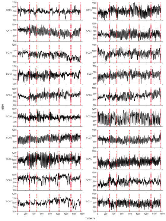
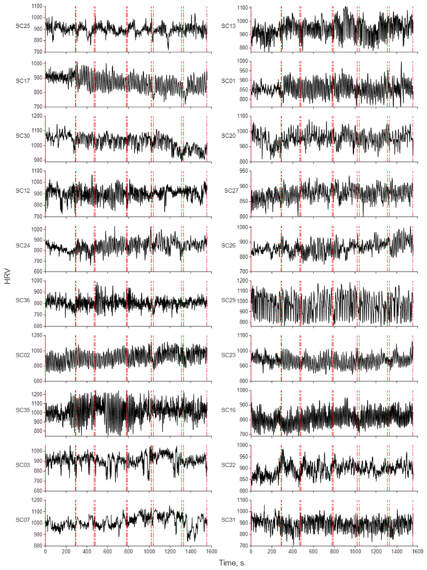
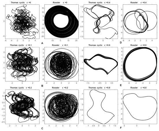
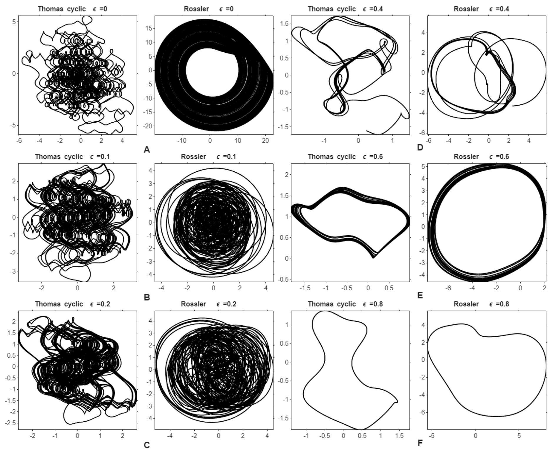
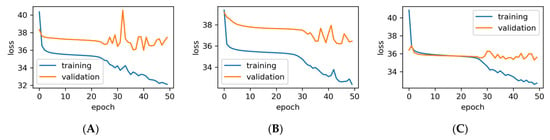
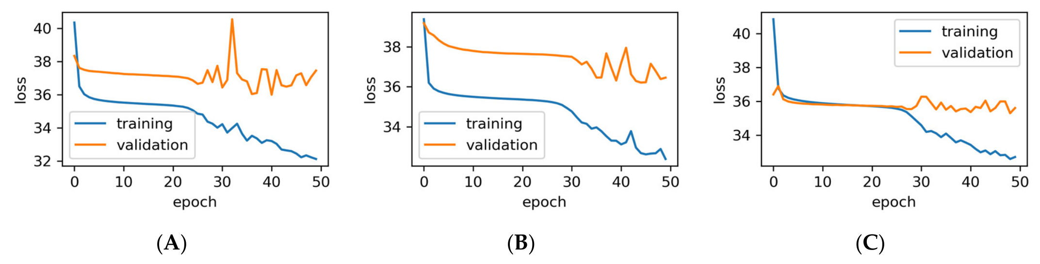
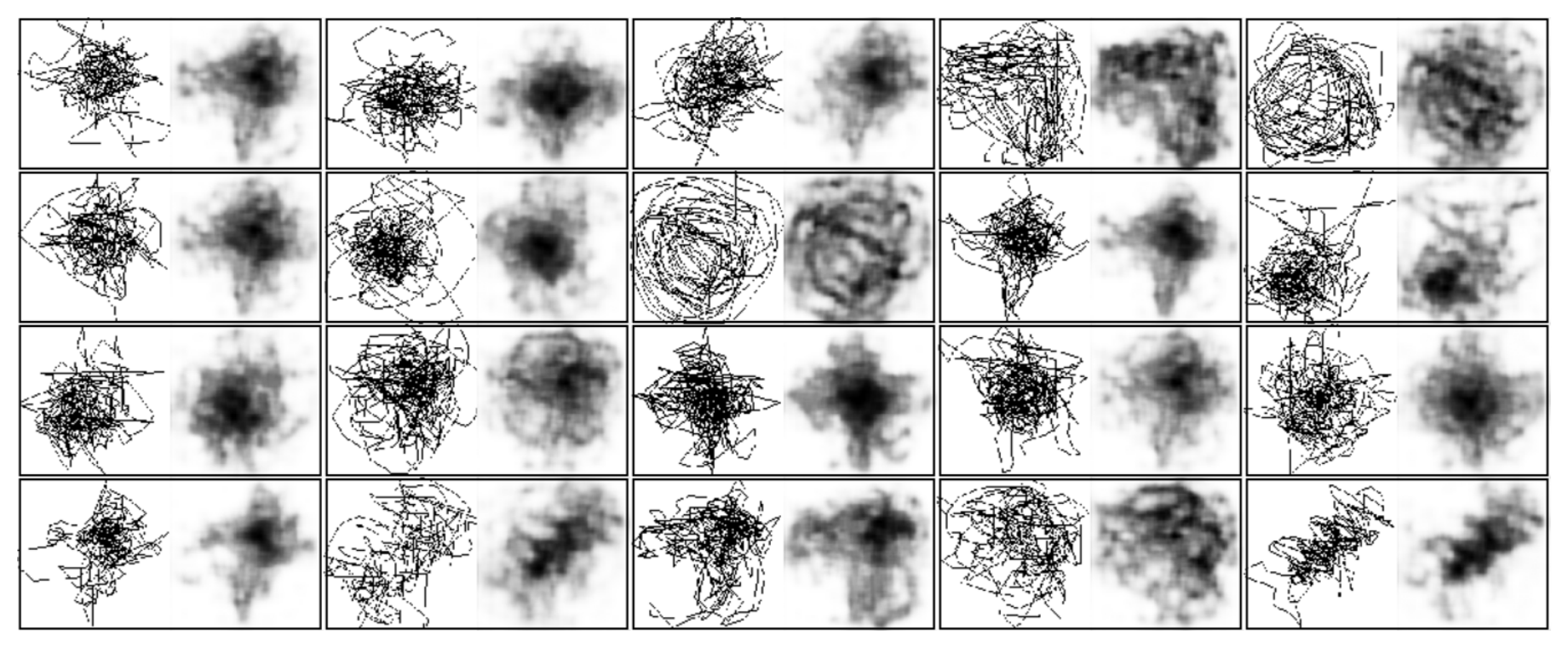
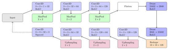
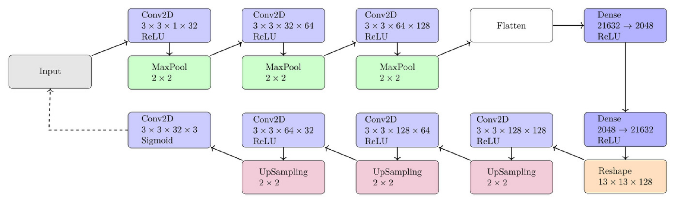
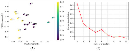
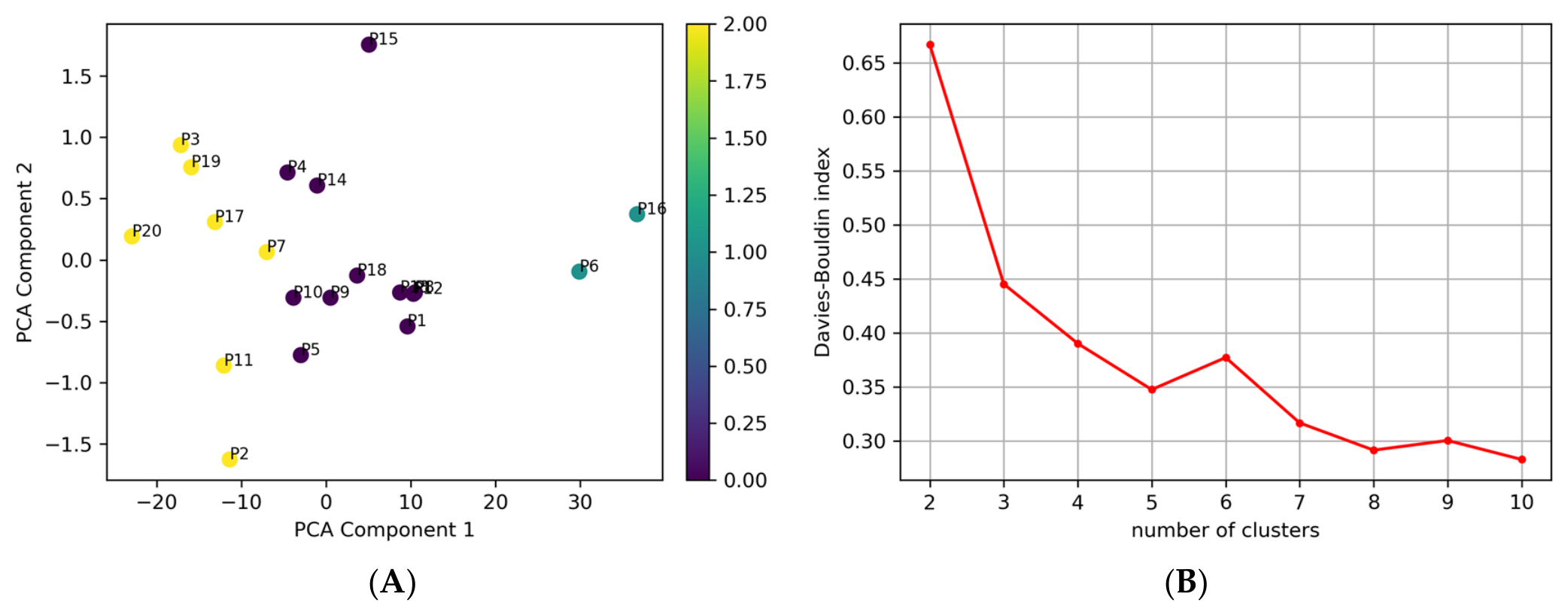
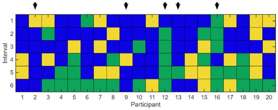
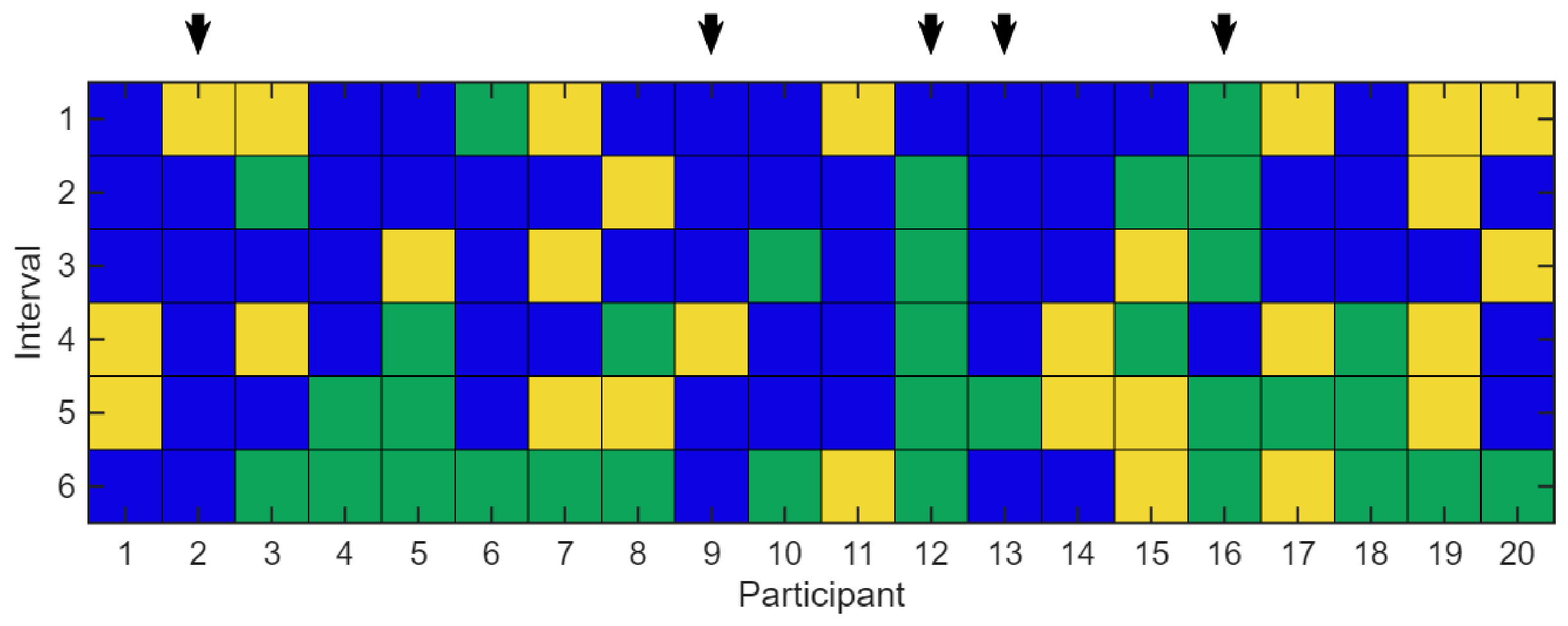
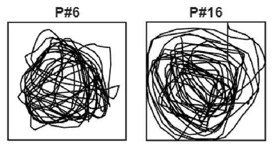
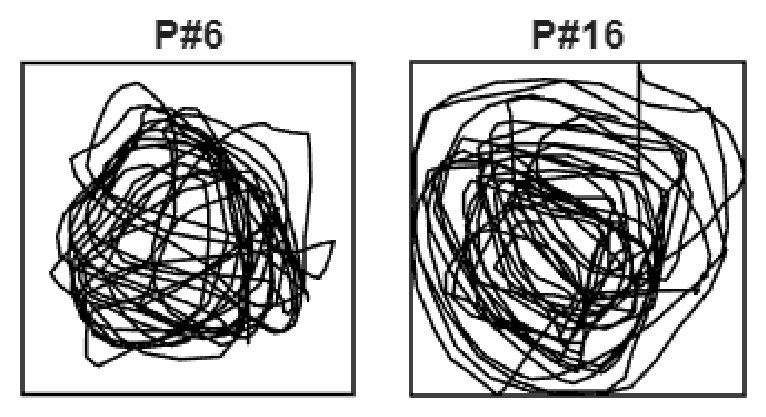
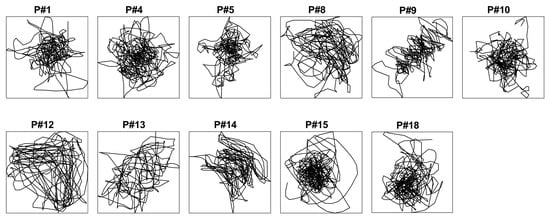
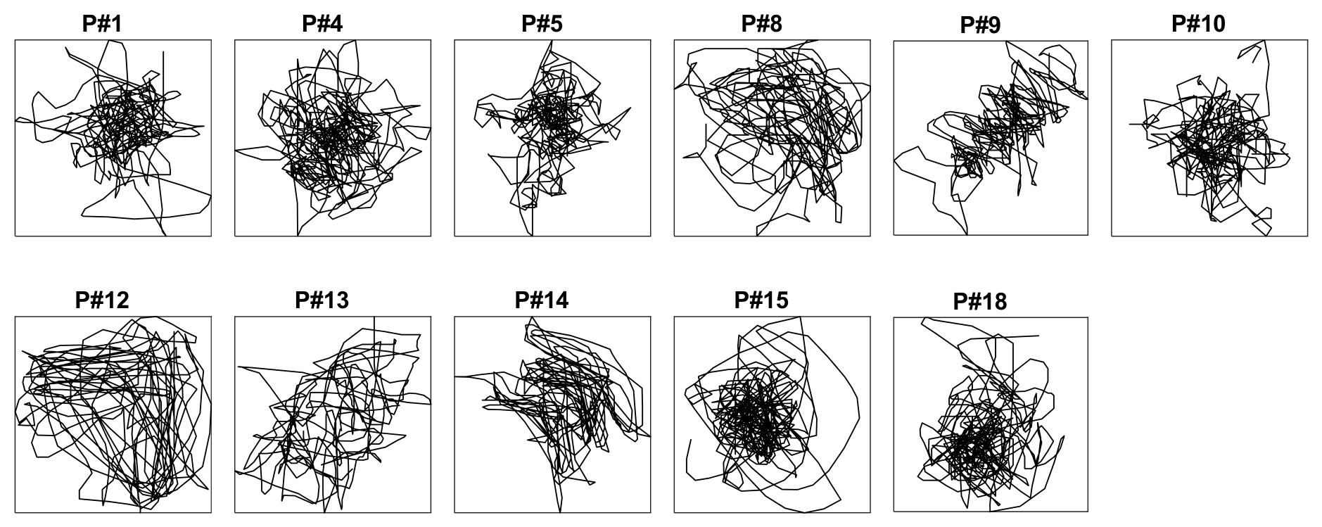


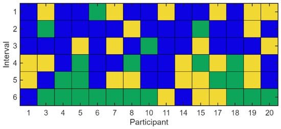
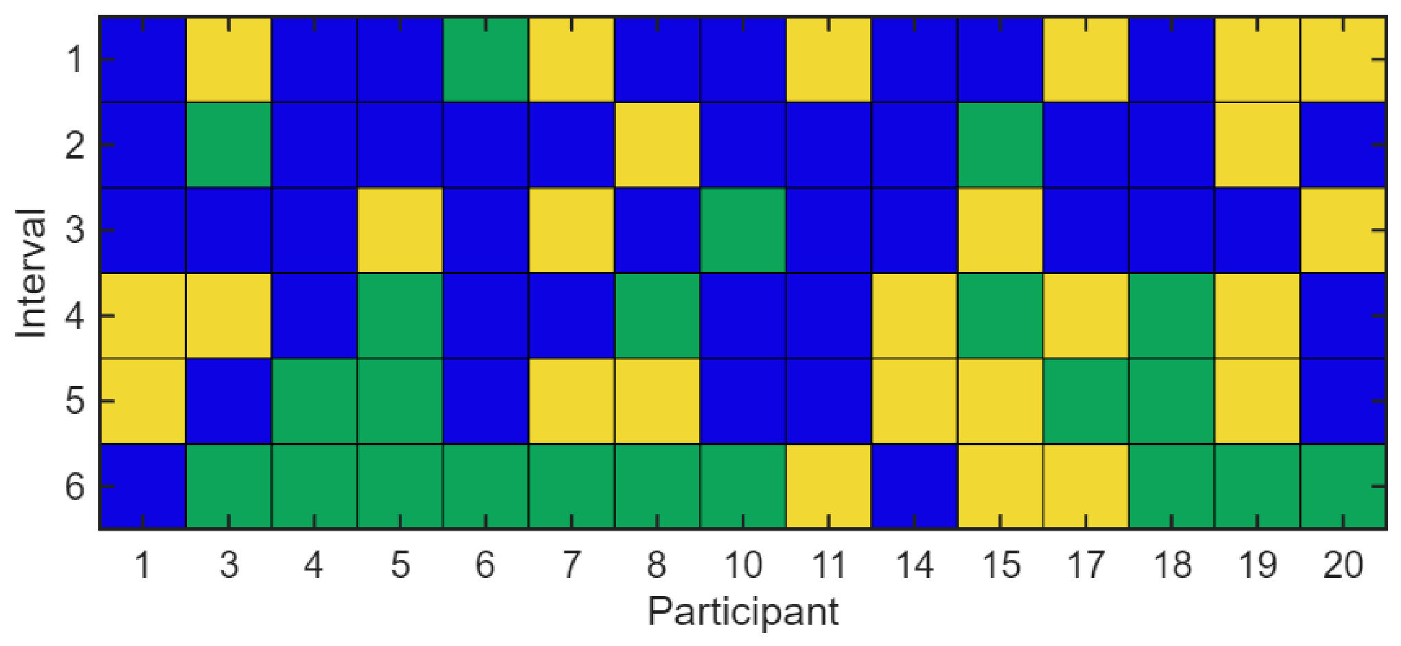
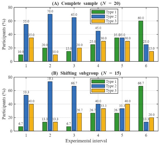
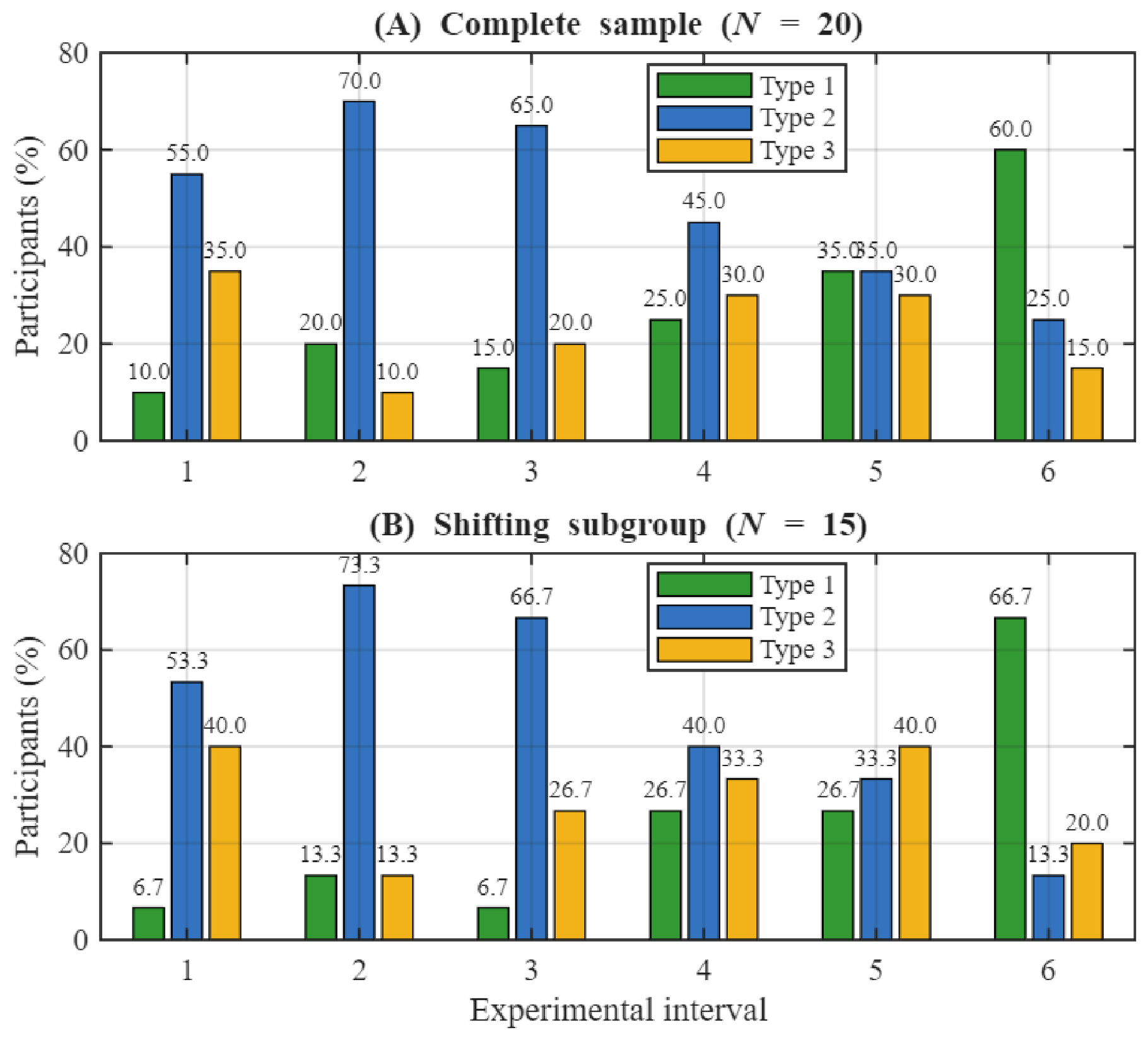

Disclaimer/Publisher’s Note: The statements, opinions and data contained in all publications are solely those of the individual author(s) and contributor(s) and not of MDPI and/or the editor(s). MDPI and/or the editor(s) disclaim responsibility for any injury to people or property resulting from any ideas, methods, instructions or products referred to in the content. |
© 2026 by the authors. Licensee MDPI, Basel, Switzerland. This article is an open access article distributed under the terms and conditions of the Creative Commons Attribution (CC BY) license.