


Abstract
Fetal electroencephalogram (fEEG) recording could address the gap of functional fetal brain testing and enable direct assessment of fetal brain status during pregnancy and labor. However, the fetal EEG signal (~1 µV) is masked by roughly 80 dB (about 10,000×) of maternal ECG and other bioelectric interferences. This synthetic-data feasibility study presents whether the fetal EEG can be recovered from the maternal abdomen surface by using the following three sensing architectures on physiologically scaled synthetic data: single electrode, dual electrode, and a concentric 28-electrode array centered over the fetal head. We show that exploiting a known geometric attenuation steering vector with a minimum-variance distortionless-response (MVDR) beamformer raises recovery correlation from ~0 to ~0.28 and improves signal-to-noise ratio (SNR) by ~67 dB. A follow-up validation replaces the synthetic EEG generator with actual neonatal EEGs recorded from the scalp, obtained from OpenNeuro ds004577 and the Helsinki Zenodo corpus. Comparable recovery performance across both datasets confirms that the synthetic feasibility conclusion generalizes to real neonatal EEG composition and behavioral characteristics. The primary evaluation is based on waveform-level engineering metrics (correlation, SNR, and RMSE), while exploratory secondary analyses assess aEEG envelopes, band-power trends, and burst detection. These analyses are not intended as clinical validation. Independent per-electrode sensor noise remains the dominant residual limiter under the homogeneous geometric model. The reported r ≈ 0.28 should not be interpreted as expected in vivo performance at all gestational ages: an intact vernix layer can add approximately 35 dB of attenuation and makes the required noise floor substantially more stringent. This analysis adds a five-layer volume-conductor analysis, misalignment, depth and impedance-drift stress tests, recording-level statistics, comparisons with classical extraction families (PCA, ICA, adaptive cancelation, and multichannel Wiener filtering), an interference-alignment sensitivity analysis, and exploratory biomarker-level analyses, which together bound the idealizations of the forward model.
1. Introduction
Perinatal brain injury is a leading cause of lifelong neurodevelopmental disability and a major contributor to neonatal morbidity and mortality [1,2]. Continuous fetal heart rate (FHR) monitoring is the standard, routine, clinical practice during prenatal visits and labor and delivery fetal assessment [1,3]. However, FHR is only an indirect surrogate for fetal brain status. FHR monitoring measures the baseline fetal heart rate, its variability, undesirable periods of slow heart rate (bradycardia) and the desirable presence of periodic faster heart rates (accelerations), allowing some inferences to be drawn regarding evolving brain injury. Unfortunately, current FHR monitoring misses many opportunities to interrupt ongoing brain injury by performing prompt cesarean section delivery. Conversely, due to its false positive interpretation, current FHR monitoring also leads to many unnecessary cesarean deliveries [1]. In contrast, the fetal electroencephalogram (fEEG) is a direct measure of brain electrical activity [1,4]. In the setting of hypoxia-ischemia, EEG’s frequency and amplitude fall and its discontinuity increases [5], progressing to an isoelectric (“flat”) tracing in severe birth asphyxia [1,6,7,8]. Fetal EEG also reveals physiologic sleep cycling and metrics of CNS maturation [6].
One of the gold standards in clinical practice of determining the neurologic status of the neonate is continuous neonatal EEG monitoring that has been studied for decades and is widely accepted as the preeminent tool to measure the functional integrity of the very young brain [9,10]. A wealth of information regarding the characteristics of normal and abnormal neonatal EEG patterns exists in preterm and full-term newborns [11].
Unfortunately, fEEG is currently unavailable for the unborn fetus, as the primary barrier to its clinical adoption is limited access [12]. Present, fEEG is only rarely recorded with scalp electrodes after rupture of the membranes near the end of the labor and delivery process [6,7]. A non-invasive, trans-abdominal route to the fEEG—usable antenatally and throughout labor—would enable continuous, direct fetal neuro-monitoring, earlier detection of hypoxic–ischemic injury, and better-targeted interventions. That clinical need motivates the abdominal electrode-array device studied here.
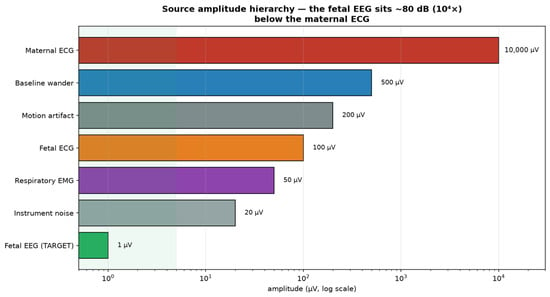
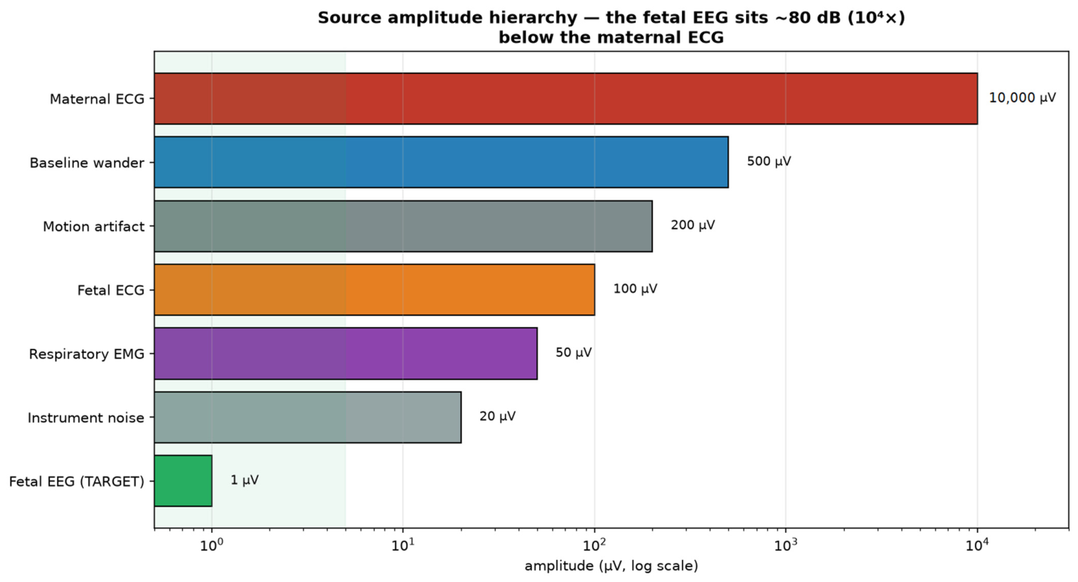
Electrical sampling from the gravid abdomen is a heavily corrupted mixture of signals including the mother’s and fetus’s bodies (e.g., ECG) [12]. The core difficulty is dynamic range and overlapping signal spectra [13]. As illustrated in Figure 1:
Figure 1.
Source amplitude hierarchy on the maternal abdomen (log scale). The fetal EEG (green) is the smallest quantity in the system by a wide margin.
- The target fetal EEG is calculated to be ~1 µV, recorded from the mother’s abdomen;
- The maternal ECG is ~10 mV—about 10,000 times larger—and spectrally overlaps the EEG frequency bands;
- Additional interferences (e.g., baseline wander, motion and EMG artifacts, fetal ECG, and respirations) all exceed the fetal EEG by 1–4 orders of magnitude;
- Per-electrode instrument noise (~2–20 µV) alone is many times larger than the target signal.
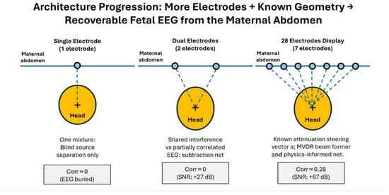
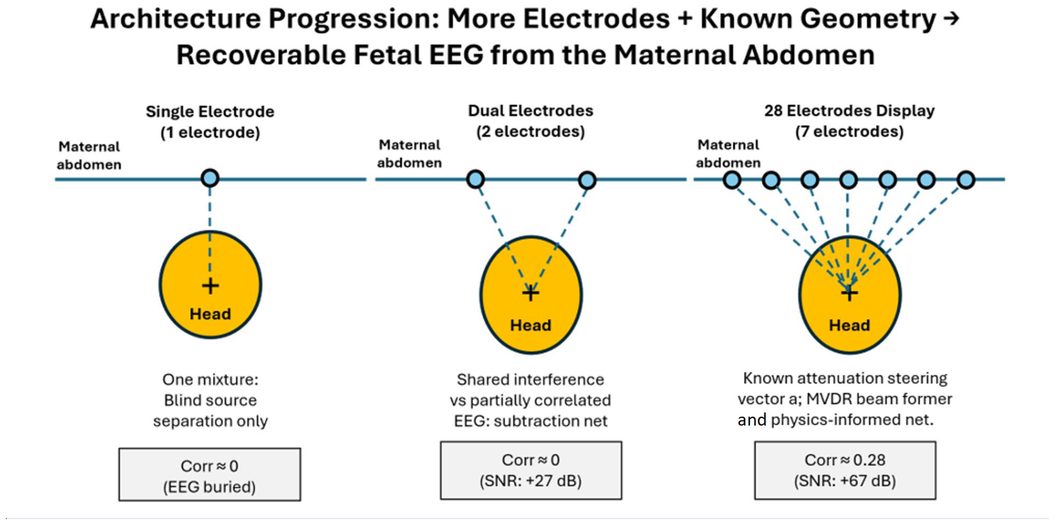
We progress through three architectures of increasing spatial diversity and test each on synthetic data with known ground truth (Figure 2). The central idea is a concentric 28-electrode array centered over the fetal head (located by ultrasound): each electrode observes the same fetal brain source attenuated by a distance fixed from geometry, yielding a known steering vector that a spatial beamformer can exploit [5]. After establishing promising synthetic results, we validate the array method using actual neonatal EEGs as injected brain sources.
Figure 2.
Architecture progression: single electrode, dual electrode, and 28-electrode concentric array with known head geometry.
2. Materials and Methods
Let x(t) ∈ ℝE denote the vector of E electrode samples at time t. The fetal EEG source s(t) reaches all electrodes through a known attenuation vector a with
where dk is the electrode-to-head-center distance and p = 2 (inverse-square, dipolar far-field). Interferences combine with independent spatial gains distinct from a. The observation model is
with n(t) lumping structured interference and sensor noise. Recovery is scored on 4 s windows (fs = 1000 Hz, 50% overlap) using Pearson correlation, SNR, and root-mean-square error (RMSE) in µV against the true s(t).
2.1. Concentric Array Device and Attenuation Model
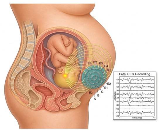
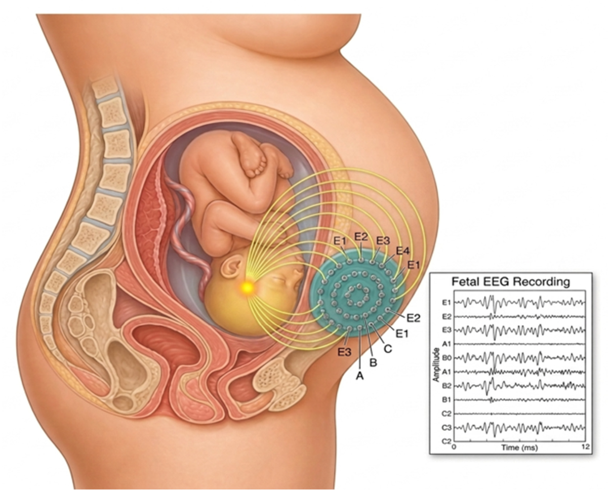
A single electrode provides one mixture and no spatial leverage, so the tiny EEG cannot be separated from co-located interference. Two electrodes add limited spatial diversity. The key insight tested here is as follows: if an electrode array is centered over the fetal head (located by ultrasound), then each electrode observes the same fetal brain source attenuated by a distance that is fixed and computable from geometry. The EEG therefore has a known spatial “steering vector”, while the interferences do not, and that asymmetry is exactly what a spatial filter (beamformer) can exploit to cancel interference and detect the actual fEEG (Figure 3) [14].
Figure 3.
A wearable concentric electrode-array patch on the maternal abdomen, positioned over the fetal head, records the trans-abdominal fetal EEG non-invasively.
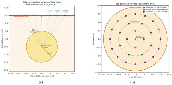
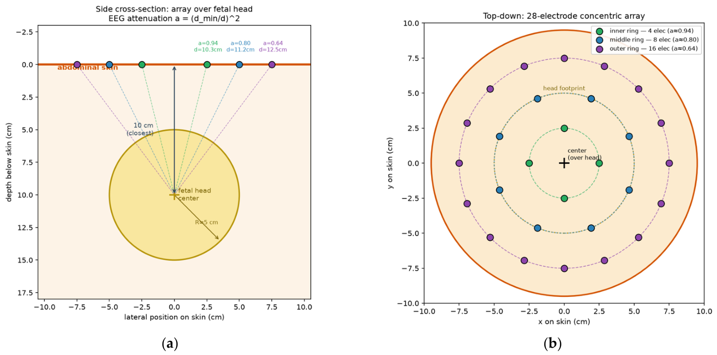
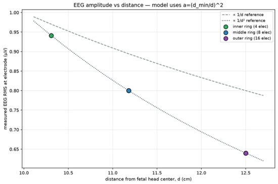
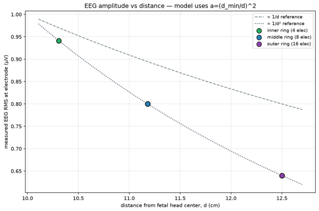
We proposed a device in which 28 electrodes are arranged in three concentric rings (4, 8, and 16 electrodes) with radii of 2.5, 5.0, and 7.5 cm, respectively, centered over the fetal head. Because the distance between the recording electrodes and the head center is fixed by geometry, the per-electrode EEG attenuation is known a priori (Figure 4). The head is modeled as a sphere of radius 5 cm with its center 10 cm below the skin. Figure 5 depicts the attenuation factors a for each electrode ring, which are a ≈ 0.94 (inner), 0.80 (middle), and 0.64 (outer). These attenuation factors are derived from the inverse-square law, which describes the far-field behavior of a current dipole in a volume conductor [15,16,17].
Figure 4.
Device schematic: (a) side cross-section showing the 5 cm head 10 cm below the skin and the per-ring distances/attenuations; (b) top-down 4 + 8 + 16 electrode layout.
Figure 5.
Verification that the measured per-electrode EEG amplitude follows the assumed inverse-square law (1/r2) with distance from the head center (d).
Validation of the 1/R2 Attenuation Assumption
The inverse-square attenuation is not arbitrary. It is the analytic far-field behavior of a current dipole in a volume conductor. The scalp potential of a current dipole obeys
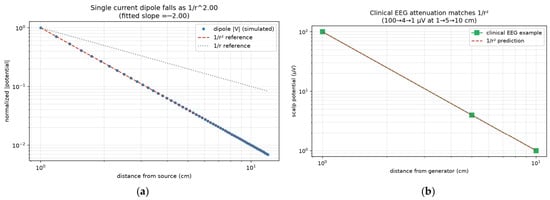
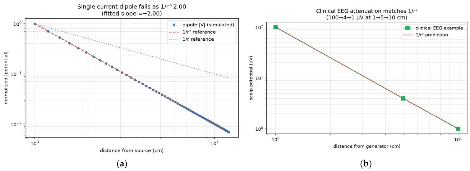
whose magnitude falls as 1/r2 [15,16]. Standard clinical electroencephalography texts state that a cortical generator producing approximately 100 µV at a distance of 1 cm is attenuated to approximately 4 µV at 5 cm and 1 µV at 10 cm within the head [17]. This inverse-square relationship provides a useful geometric reference to record transabdominal fetal EEG. However, the signal must additionally traverse the fetal skull, vernix caseosa, amniotic fluid, uterine tissues, and the maternal abdominal wall [18,19]. Therefore, the assumed fetal EEG amplitude of approximately 1 µV should be regarded as an optimistic geometric estimate rather than an established physiological value. Figure 6 reproduces both validation results as follows: a simulated current dipole yields a fitted log-log slope of −2.00, and the clinical example lies exactly on the theoretical 1/r2 attenuation curve (a monopolar source would fall only as 1/r; if the net dipole moment cancels, the leading term is a quadrupole falling as 1/r3).
Figure 6.
Validation of the inverse-square law: (a) a simulated current dipole falls as 1/r2; (b) the textbook clinical EEG attenuation example matches the 1/r2 prediction.
2.2. Extraction Methods
2.2.1. Baselines
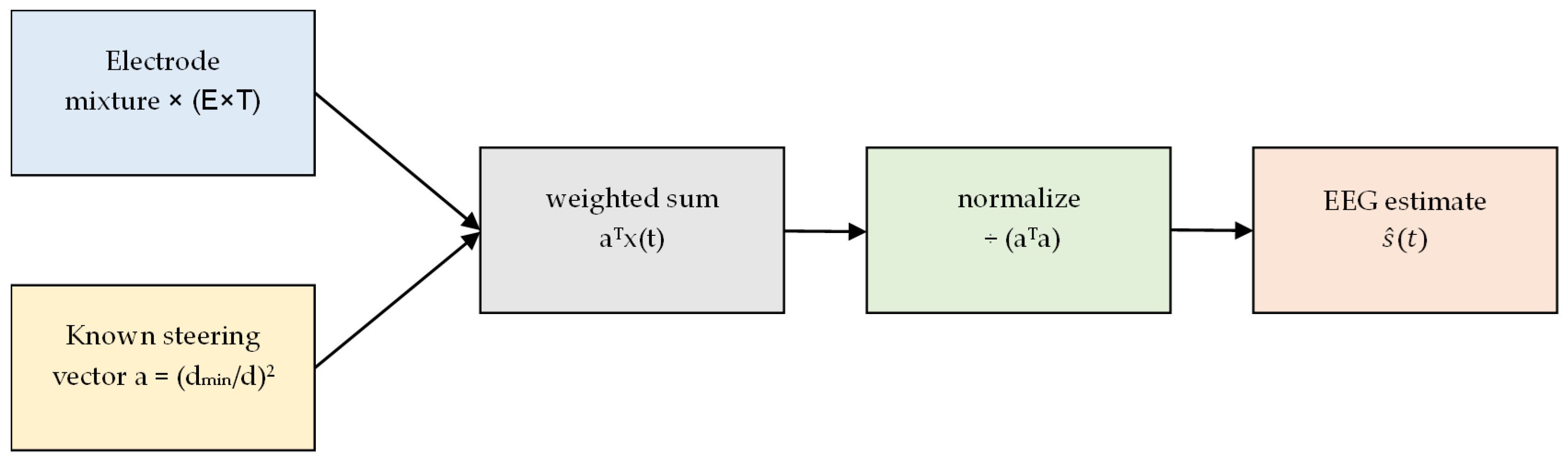
The raw inner-electrode baseline selects k* = argmax ak and forms (Appendix B.2)
The matched filter (least squares) gives (Appendix B.3)
but does not null structured interference.
A dual-electrode DualRTCN (Appendix B.5) predicts shared interference on channel 1 and subtracts it, improving SNR without waveform-level correlation.
2.2.2. MVDR Beamformer
The minimum-variance distortionless-response (MVDR) beamformer minimizes output variance subject to unit gain on direction a:
where R is the spatial covariance [14]. Diagonal loading (ε = 10−6) and float64 inversion are required for the 60 dB dynamic range [20] (Appendix B.4).
2.2.3. ArrayRTCN
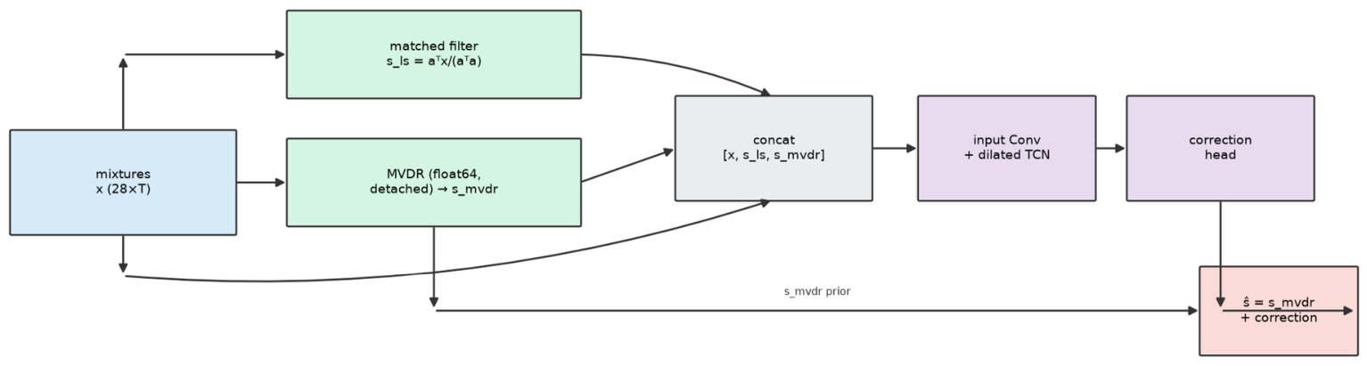
ArrayRTCN concatenates the 28-channel mixture with matched-filter and MVDR estimates and learns a residual correction
initialized at MVDR. In the linear mixture regime, it matches MVDR. The temporal backbone follows the generic Temporal Convolutional Network (TCN) architecture [21], while the residual prediction strategy is inspired by deep residual learning [22] (Appendix B.6).
2.2.4. Classical Comparison Methods
To test whether the known geometric steering vector is the decisive prior, the synthetic held-out windows were also processed with four established extraction families. PCA retained the first principal component of each 28-channel window. FastICA used 10 components, a maximum of 500 iterations and a tolerance of 10−3; the component with the largest absolute correlation to the true source was retained (oracle selection, an upper bound that no blind system reaches in practice). Adaptive cancelation used a 21-tap least-squares FIR filter predicting the inner electrode from the outer-ring average; the residual is the EEG estimate. The GEVD rank-1 multichannel Wiener filter used the oracle interference-plus-noise covariance formed from the known ground-truth decomposition, with 10−9 relative diagonal loading. No additional preprocessing beyond the shared MAD-normalized 4 s windows of Appendix B.1 was applied.
2.3. Assumptions
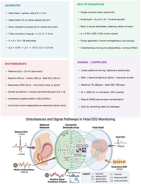
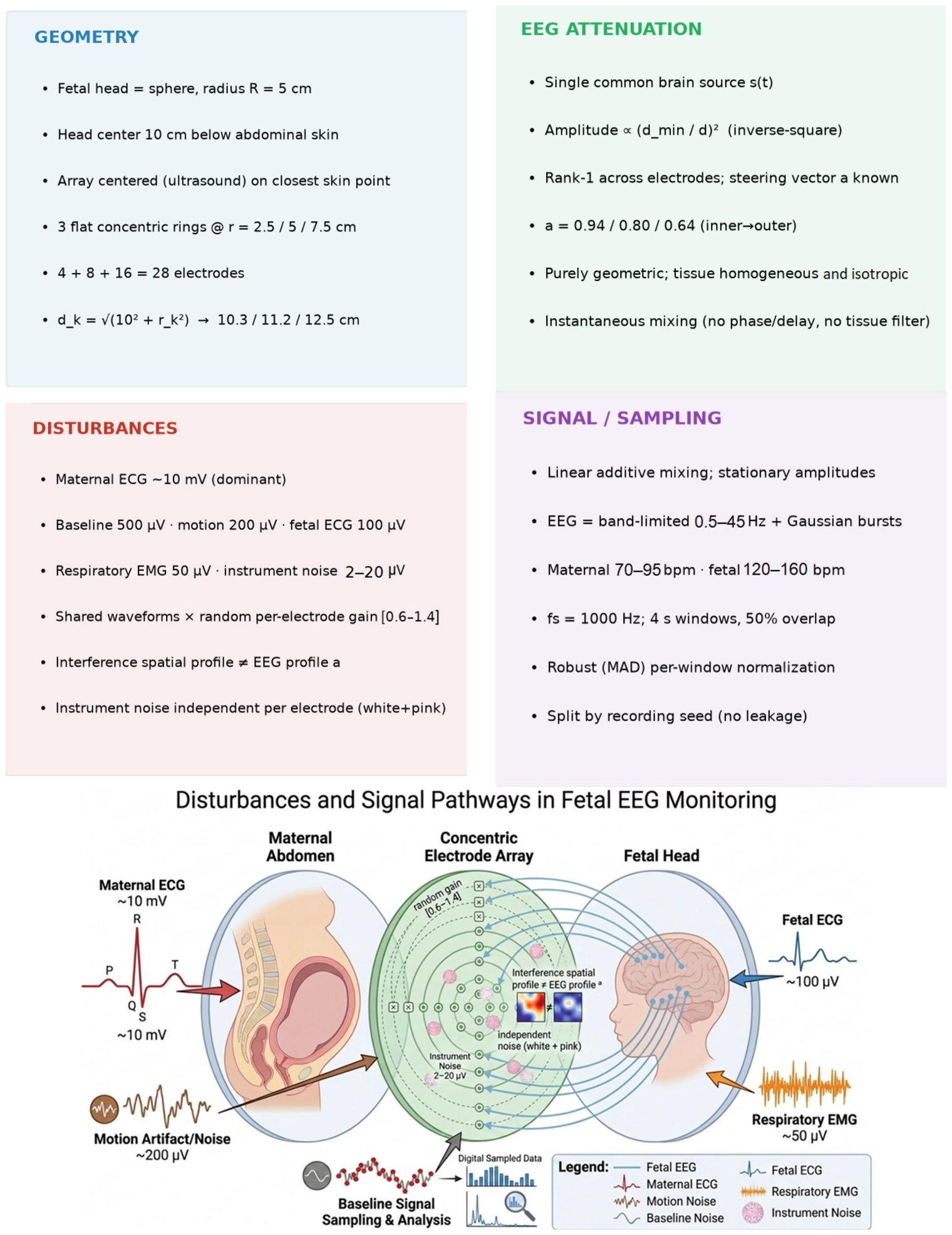
This study is based on the explicit modeling assumptions presented in Figure 7. These are idealizations chosen to isolate the spatial-separability question. These assumptions establish a controlled first-order framework for evaluating the proposed beamforming approach.
Figure 7.
Catalog of modeling assumptions, grouped by category. a denotes the fetal EEG steering vector.
2.3.1. Geometry
To establish a tractable analytical model while preserving the dominant spatial characteristics of fetal EEG propagation, the fetal head was approximated by a spherical geometry and positioned directly beneath the center of the electrode array. Ultrasound localization was expected to identify the abdomen location closest to the fetal head, allowing the array to be centered directly over the target region. This configuration provides a known geometric relationship between the fetal source and each electrode, from which the steering vector required by the beamformer can be computed.
- The fetal head is a sphere of radius R = 5 cm;
- The head center lies 10 cm beneath the abdominal skin, along the array’s central normal;
- The array is positioned via ultrasound, so its center is the abdominal skin point closest to the head center;
- Three flat, concentric rings on the skin at radii 2.5, 5.0, 7.5 cm with 4, 8, 16 electrodes (28 total), angularly staggered between rings;
- The electrode-to-head-center distance is given by
Which is approximately 10.3, 11.2, and 12.5 cm for the inner, middle, and outer electrode rings, respectively.
These geometric assumptions represent an idealized first-order approximation rather than an exact clinical configuration. In practice, fetal movement, head descent during labor, variations in amniotic-fluid thickness, and imperfect ultrasound localization continuously alter the distance and alignment between the fetal head and the electrode array. Consequently, the true steering vector may differ from the assumed one, resulting in steering-vector mismatch. Because the MVDR beamformer relies on an accurate steering vector to preserve the desired signal while suppressing interference, such mismatch can reduce recovery performance by partially attenuating the target EEG. The present study therefore evaluates the proposed method under idealized geometric conditions to establish baseline feasibility. Assessing robustness to geometric uncertainty and developing beamforming strategies that are less sensitive to steering-vector mismatch remain important directions for future work. This robustness assessment has now been performed (Section 3.9): recovery degrades by less than 30% for lateral misalignment up to 5 cm and array tilt up to 20°, while depth misestimation is the sensitive axis, dominated by the physical 1/d2 amplitude loss rather than by steering mismatch.
2.3.2. EEG Attenuation
The fetal EEG propagation model used in this study is based on a first-order geometric approximation. The fetal brain activity is represented by a single dominant source whose amplitude decreases with distance according to the inverse-square behavior of a current dipole in the far field. This simplified model isolates the influence of source geometry and enables analytical computation of the steering vector required by the beamformer.
- A single common fetal brain source, s(t), reaches all electrodes (rank-1 spatial model);
- Amplitude attenuates according to Equation (1), with d_min = 10 cm and p = 2 (inverse-square, dipolar far-field). The exponent p is configurable, allowing alternative attenuation models (e.g., 1/d, corresponding to p = 1);
- Resulting attenuation factors: (inner), (middle), and (outer), with the strongest and weakest signals observed at the inner and outer rings, respectively;
- Attenuation is purely geometric; tissue is treated as a homogeneous, isotropic, and non-dispersive volume conductor;
- Mixing is instantaneous (no inter-electrode propagation delay or frequency-dependent tissue filtering);
- The steering vector a is known to the algorithm (geometry from ultrasound).
These assumptions intentionally neglect several biological factors known to influence transabdominal bioelectric signal propagation. In particular, the fetal skull exhibits relatively low electrical conductivity, whereas the amniotic fluid is highly conductive and can redistribute current before it reaches the maternal abdomen. In addition, from approximately the third trimester, the fetus becomes coated with vernix caseosa, a highly resistive lipid layer that has long been recognized as a major cause of the attenuation of transabdominal fetal ECG. Consequently, the propagation path is neither homogeneous nor isotropic, and these layered, gestational-age-dependent effects may dominate the simple geometric attenuation assumed in this study. Such effects can alter both the signal amplitude and the spatial steering vector used by the MVDR beamformer. Therefore, the proposed propagation model should be regarded as a first-order approximation intended to evaluate the feasibility of the spatial recovery framework. Incorporating multilayer volume-conductor models that explicitly account for the fetal skull, vernix caseosa, amniotic fluid, and maternal tissues will be an important direction for future work. A first analytic step is provided in Section 3.9 as follows: a five-layer concentric-sphere model shows that the steering-vector shape remains cosine-aligned (greater than 0.98) with the 1/r2 assumption, whereas an intact vernix layer attenuates the abdominal EEG amplitude to approximately 2% of the geometric prediction (about −35 dB), with negligible spectral distortion across 0.5–45 Hz.
2.3.3. Disturbances/Sources
The simulated abdominal recordings were generated by linearly combining the target fetal EEG with the dominant physiological and instrumental interference sources anticipated to be encountered in abdominal bioelectric recordings. To evaluate the proposed beamforming framework under controlled conditions, each interference source was assigned a spatial profile distinct from that of the fetal EEG. This assumption ensures that the desired signal and the interfering sources remain spatially distinguishable, allowing the MVDR beamformer to exploit differences in their steering vectors for interference suppression.
- Maternal ECG ~10 mV (dominant); baseline wander 500 µV; motion artifacts 200 µV; fetal ECG 100 µV; respiratory EMG 50 µV; instrument noise 2–20 µV; fetal EEG ~1 µV at the array center;
- Each interference source is modeled as a shared waveform mixed onto all electrodes with independent random gains in [0.6, 1.4], yielding a spatial profile distinct from and uncorrelated with the fetal EEG steering vector a;
- Instrument noise is independent per electrode (mixed white and pink noise);
- All sources combine by linear superposition; amplitude scales are stationary;
- Heart rates: maternal 70–95 bpm, fetal 120–160 bpm; respiration 14–28 breaths/min (randomized per recording).
This interference model represents an idealized first-order approximation. In particular, the maternal ECG originates from a relatively distant source, and its amplitude distribution across the approximately 15 cm abdominal array may exhibit only a shallow spatial gradient. Consequently, its steering vector could partially align with that of the fetal EEG, reducing the ability of the MVDR beamformer to place deep spatial nulls while preserving the desired signal. Furthermore, the present model does not include several clinically important interference sources, such as bowel and uterine electromyographic activity (electrohysterogram), or maternal abdominal wall EMG, all of which are highly non-stationary and may become dominant during labor. These factors were intentionally omitted to isolate the fundamental spatial recovery problem. Extending the interference model to include more realistic physiological sources remains important future work. Crucially, the present generator imposes spatial distinctness as follows: each interferer is mixed with independent random gains in [0.6, 1.4], so its spatial profile is drawn independently of the EEG steering vector a, rather than being measured from the maternal abdomen. Spatial separability is therefore a modeling assumption, not an empirical demonstration. Section 3.9 withdraws that assumption by sweeping the cosine similarity between the maternal-ECG gain vector and a.
2.3.4. Signal Model and Processing
The fetal EEG was modeled using a simplified signal generator designed to reproduce the principal spectral characteristics of neonatal EEG while providing a controlled reference signal for quantitative evaluation. The synthetic EEG consists of a band-limited background activity combined with transient oscillatory bursts, enabling objective assessment of signal recovery using known ground truth.
- Fetal EEG = band-limited background (0.5–45 Hz) plus Gaussian-windowed sinusoidal bursts (3–12 Hz);
- Sampling rate fs = 1000 Hz; analysis in 4 s windows with 50% overlap;
- Per-window robust (median-absolute-deviation) normalization to handle the mV-scale dynamic range;
- Train/validation/test split by recording seed to prevent leakage.
The utilized signal model represents a simplified approximation of fetal EEG and does not explicitly reproduce several physiologically important waveform morphologies observed in preterm and fetal recordings. In particular, immature EEG is characterized by discontinuous background activity, prominent slow frequency delta activity, and age specific delta brushes, all of which are important electrographic markers of early brain development. These characteristic patterns are not explicitly represented by the present band-limited background and Gaussian-burst generator. Furthermore, the most informative low-frequency EEG components overlap the spectral range occupied by baseline wander and respiratory interference, making their recovery particularly challenging. Consequently, the current evaluation should be regarded as demonstrating recovery of broadband EEG activity rather than clinically specific waveform features. Exploratory burst-detection and band-power analyses are now reported in Section 3.9; they remain secondary engineering endpoints, not clinical validation. Future work still requires physiologically realistic fetal generators (discontinuous background, delta brushes) and true transabdominal recordings.
2.4. Data
2.4.1. Synthetic Data
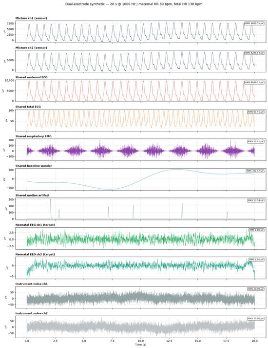
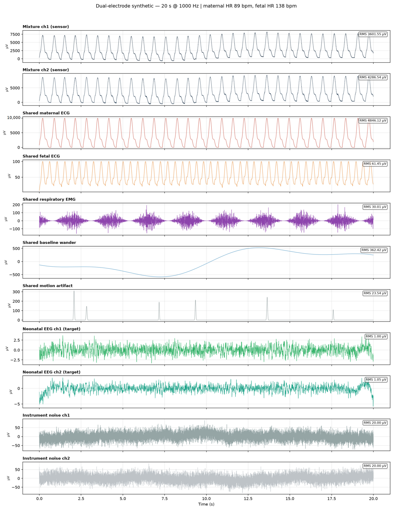
All experiments use a physiologically scaled synthetic generator so that ground truth is known exactly and recovery can be measured against the true EEG source. Each disturbance has a distinct temporal/spectral signature (Figure 8).
Figure 8.
Decomposition of a two-electrode recording into its shared sources and per-electrode EEG/noise components (µV). Note the maternal ECG dwarfs all else.
Table 1 summarizes the components and parameters of the synthetic recordings, including maternal ECG (~10 mV), fetal ECG, baseline wander, motion artifacts, respiratory EMG, 2 µV per-electrode noise, and a ~1 µV fetal EEG consisting of band-limited background activity and transient bursts.
Table 1.
Synthetic source taxonomy and physiologic amplitude scales.
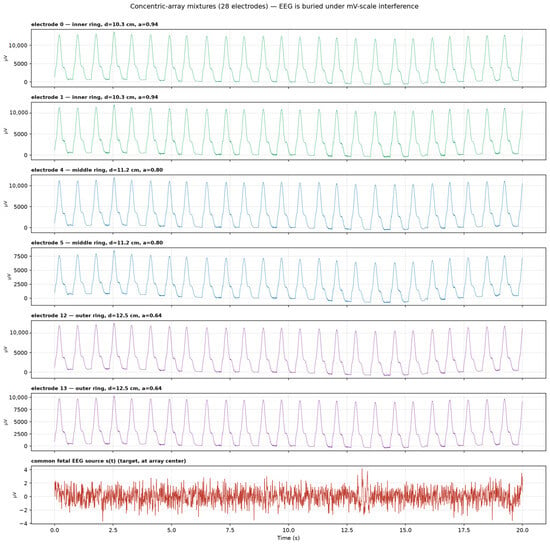
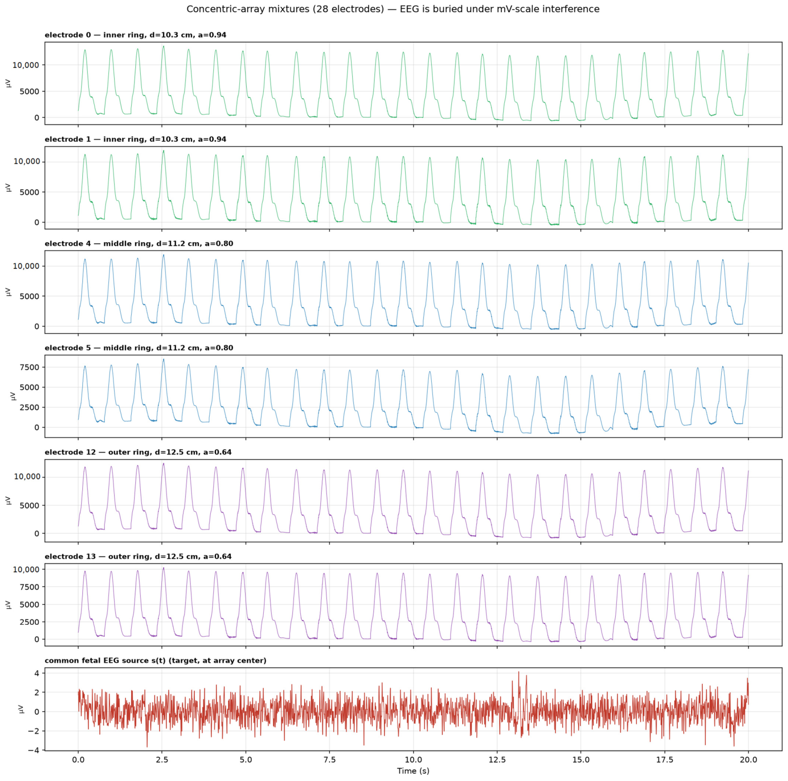
Figure 9 illustrates the simulated recordings acquired from the proposed 28-electrode concentric array. As can be seen, the target fetal EEG is almost completely buried beneath much larger amplitude interference, including maternal ECG and other physiological and non-physiologic (e.g., motion) artifacts, making direct visual identification of the fetal EEG nearly impossible.
Figure 9.
Example electrode mixtures from the 28-electrode array (one per ring) versus the common fetal EEG source s(t). The fEEG is not distinguishable in the raw traces.
2.4.2. Published Clinical Neonatal EEG Datasets
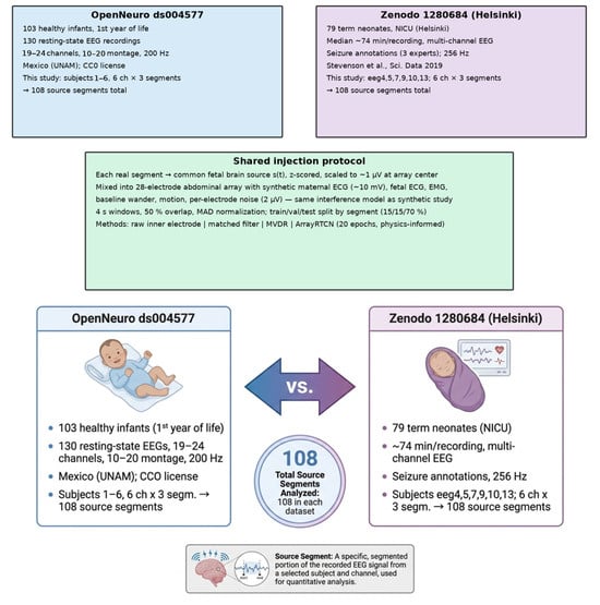
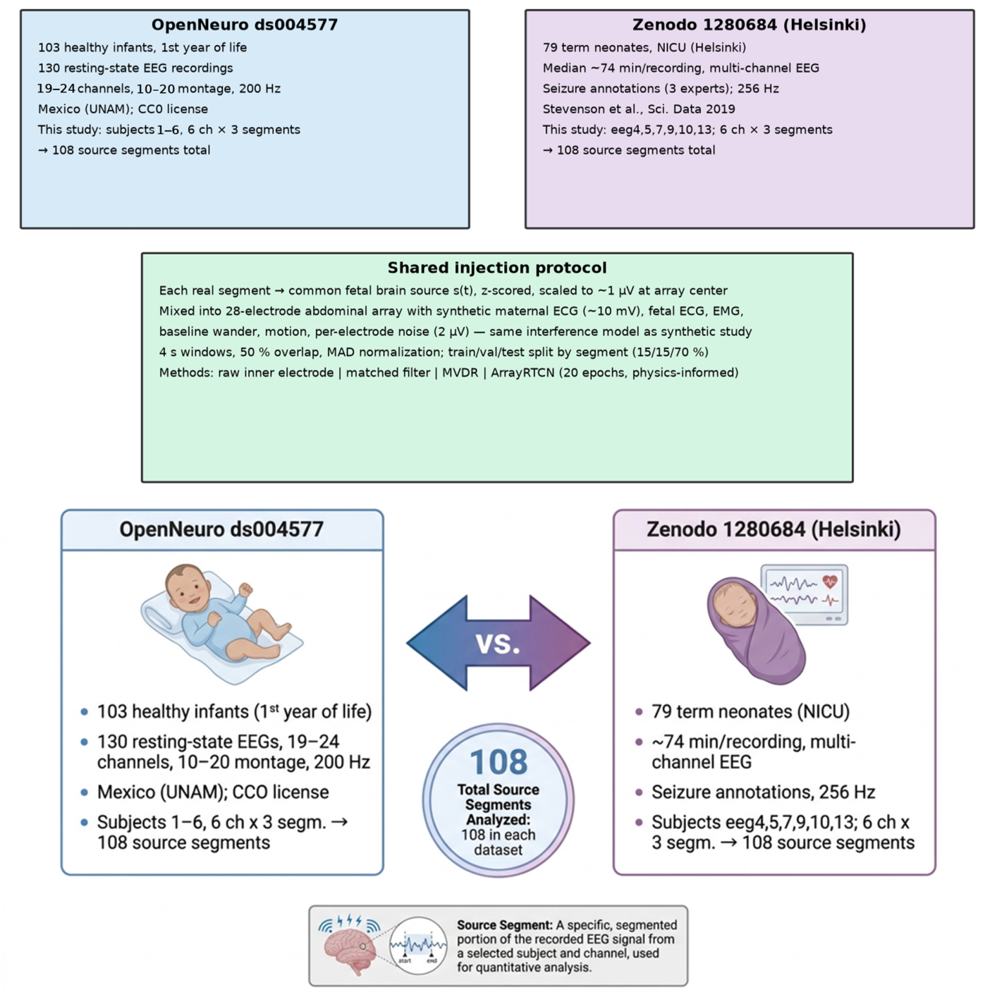
OpenNeuro ds004577 provides resting-state infant EEG (103 subjects, 200 Hz) [23,24]. Zenodo 1280684 provides Helsinki NICU neonatal EEG with seizure annotations (256 Hz) [25]. For each database we extract 108 source segments (6 recordings × 6 channels × 3 segments). Each 20 s segment is band-limited (0.5–45 Hz), resampled to 1 kHz, z-scored, scaled to ~1 µV at the array center, distributed via steering vector a, and mixed with the same synthetic interference used in the synthetic dataset (Figure 10 and Figure 11). Windowing at 4 s with 50% overlap yields 9 windows per segment and 972 windows per corpus, split 684/144/144 into train/validation/test. The held-out test cache contains 144 windows from 16 held-out source segments, not 16 independent subjects: the six original recordings remain the only independent biological units. Cluster-bootstrap inference resamples those 16 test-segment identifiers so that windows from the same segment are not treated as independent (Section 3.9). The synthetic test split comprises 2 recordings/18 windows (Appendix A). These statistics should be read as recording- or segment-level feasibility evidence, not population-level clinical evidence.
Figure 10.
End-to-end real-EEG injection and extraction pipeline.
Figure 11.
Real EEG databases and shared injection protocol.
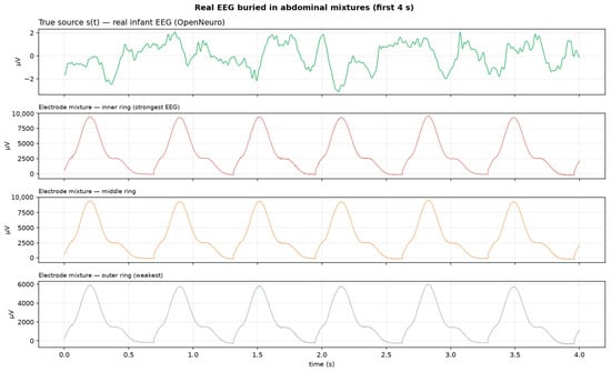
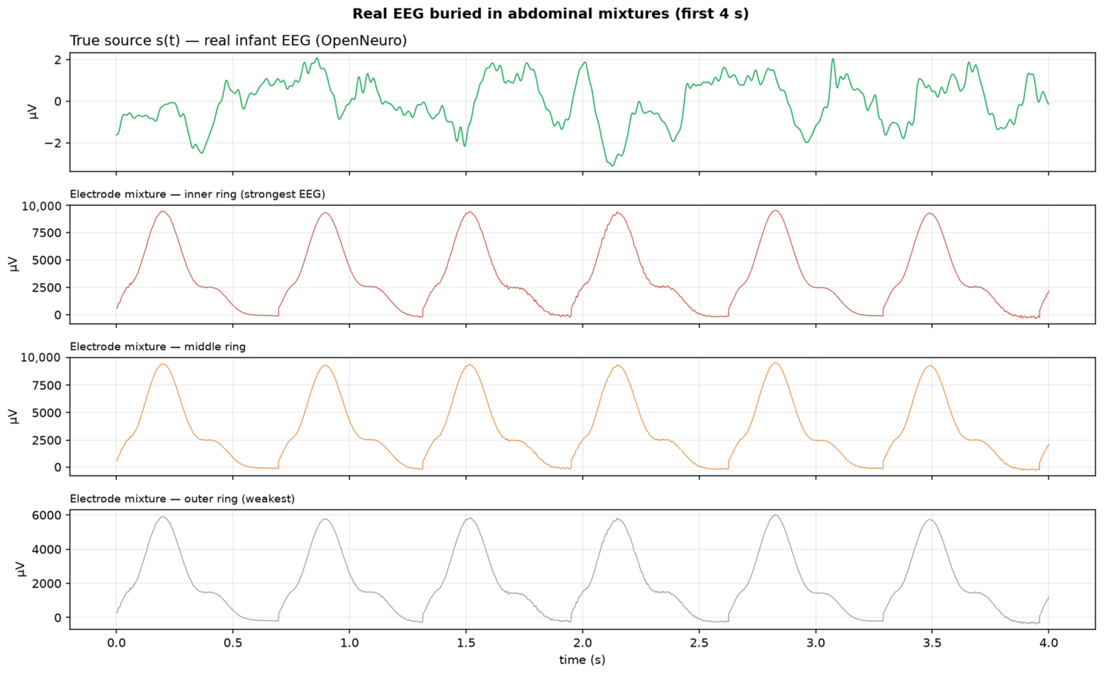
Figure 12 shows the first 4 s of an actual neonatal EEG after the addition of the simulated abdominal mixtures. The EEG signal is virtually concealed by extraneous high-amplitude interference, making direct visual identification of the underlying brain activity essentially impossible.
Figure 12.
Real infant EEG buried in abdominal mixtures (first 4 s).
3. Results
3.1. Single Electrode (Baseline)
In this case, there is only a single observed mixture; therefore, only blind source separation techniques can be applied. However, because the fetal EEG signal is heavily contaminated by various artifacts and interfering sources, it remains buried within the composite signal. As a result, accurate recovery of the EEG component is not possible, leading to a recovery correlation close to zero.
3.2. Dual Electrode
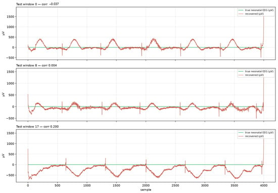
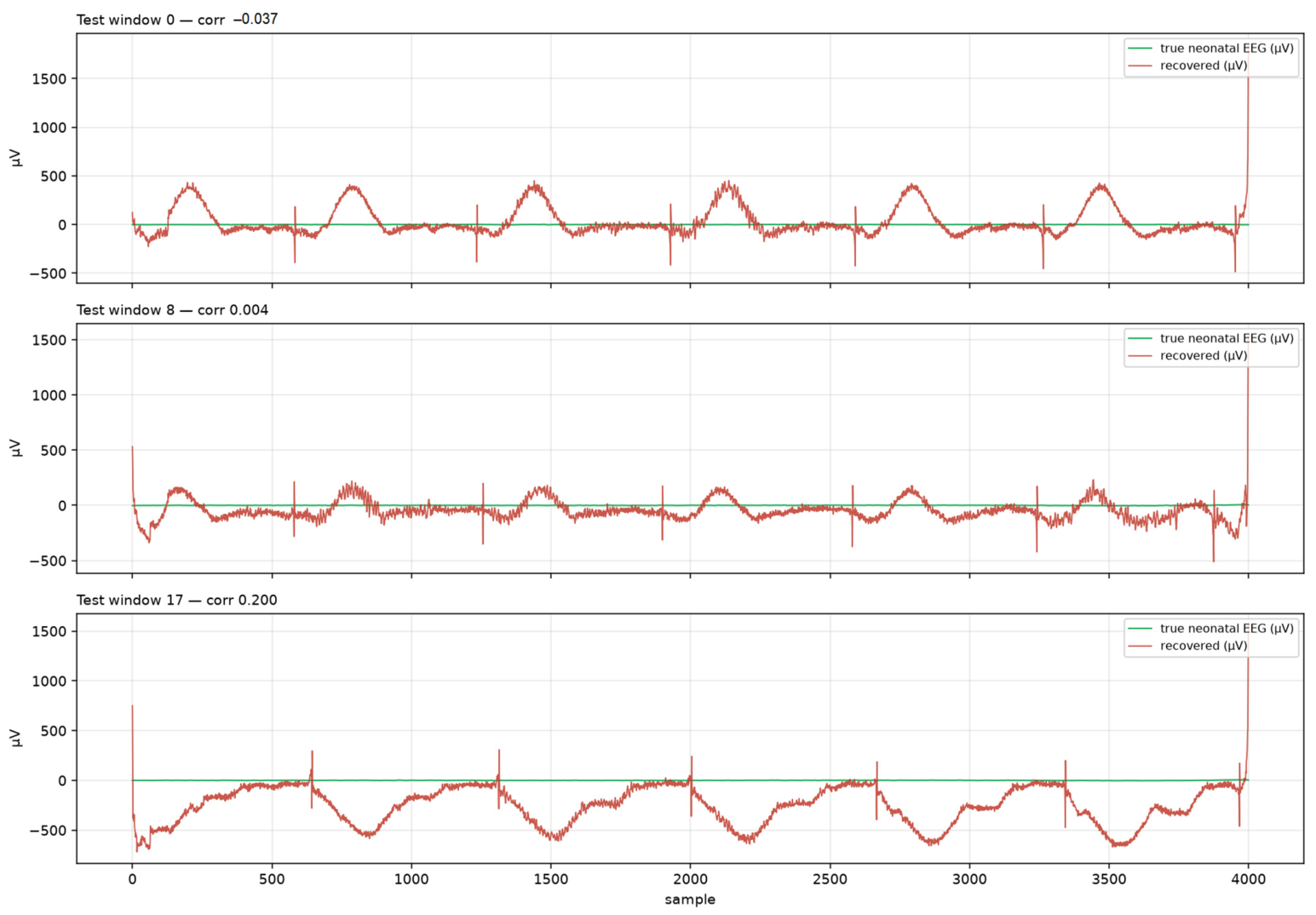
There are two electrodes with shared interferences (different gains) and partially correlated EEG (correlation beta = 0.7). A residual temporal CNN (DualRTCN) predicts the shared interference on channel 1 and subtracts it. This improves SNR by ~27 dB versus the raw mixture. However, as indicated in Figure 13, it does not yet yield waveform-level correlation, being limited by independent noise and the absence of a known spatial model.
Figure 13.
Dual-electrode recovered EEG vs. ground truth on test windows.
3.3. 28-Electrode Concentric Array
The EEG is a rank-1 source with known steering vector a. The following two estimators exploit this:
- MVDR/LCMV beamformer: The beamformer described in Section 2.2.2 preserves the desired signal with unit gain while suppressing high-variance interference. Double-precision covariance matrix inversion and a small diagonal loading factor (10−6) were used to maintain numerical stability over the 60 dB dynamic range;
- ArrayRTCN: As explained in Section 2.2.3, the temporal CNN receives the matched-filter and MVDR estimates as physics-based priors and predicts a residual correction to the MVDR output.
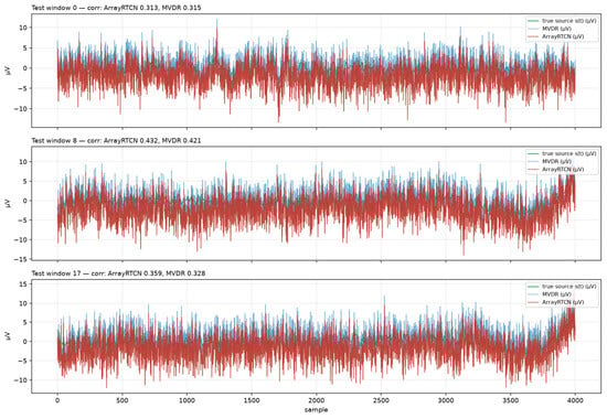
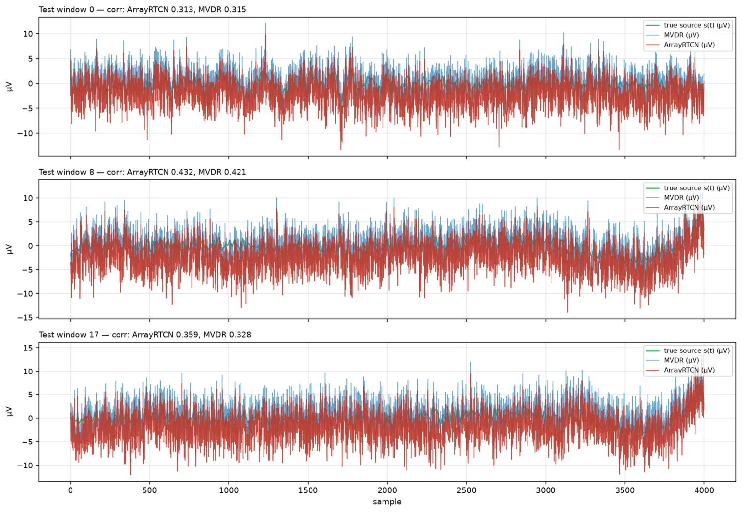
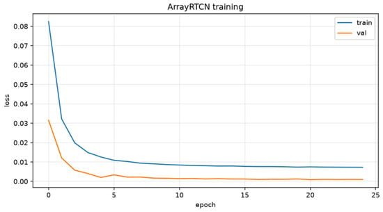
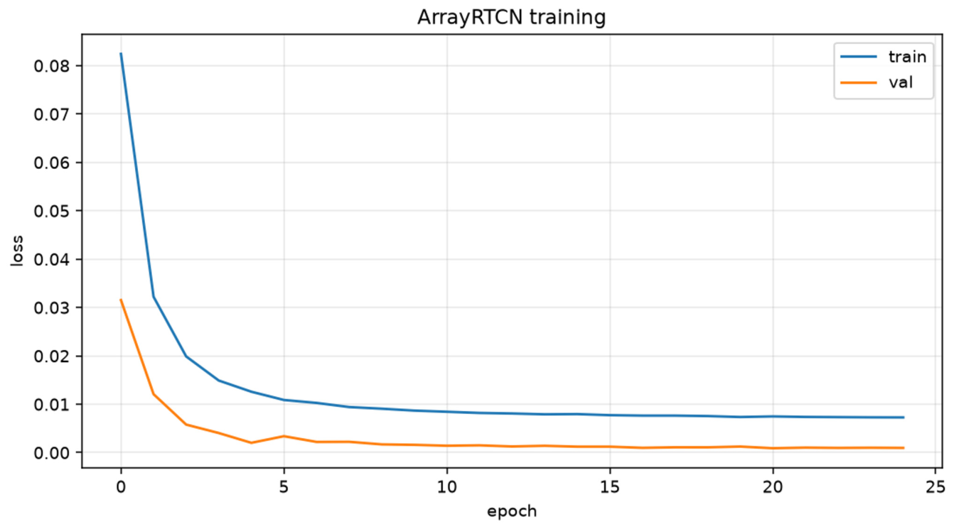
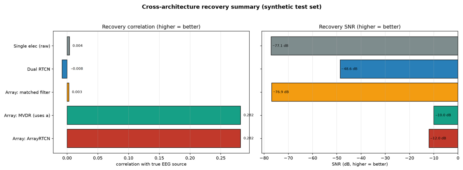
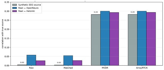
On the synthetic dataset, the raw inner electrode and the matched filter recover essentially nothing (r ≈ 0.004). In contrast, the MVDR beamformer increased the correlation to r ≈ 0.282 and improved the SNR by ~67 dB versus the raw baseline. ArrayRTCN achieved performance comparable to that of the MVDR beamformer (r ≈ 0.282), as expected when the optimal estimator is close to linear (Figure 14). The training and validation loss curves for ArrayRTCN are shown in Figure 15.
Figure 14.
Array recovery: true source s(t) (green) vs. MVDR (blue) and ArrayRTCN (red). Per-window correlation 0.282.
Figure 15.
ArrayRTCN training/validation loss.
3.4. Synthetic Test Set Results
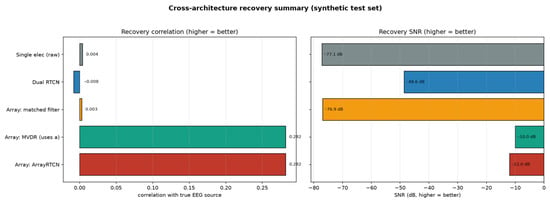
Recovery performance was evaluated against the ground-truth EEG signal on held-out test windows using the Pearson correlation coefficient, SNR, and RMSE (µV). Table 2 summarizes recovery on held-out synthetic test windows. As expected, the single electrode and a naive weighted average recover essentially nothing, while the MVDR beamformer substantially improved performance by exploiting the known spatial attenuation profile (Figure 16).
Table 2.
Recovery metrics across architectures (synthetic held-out test set).
Figure 16.
Cross-architecture recovery summary. MVDR and ArrayRTCN (which use the known attenuation profile) are the only methods that recover genuine EEG activity.
3.5. What Limits Recovery?
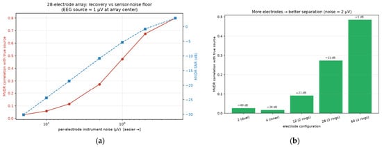
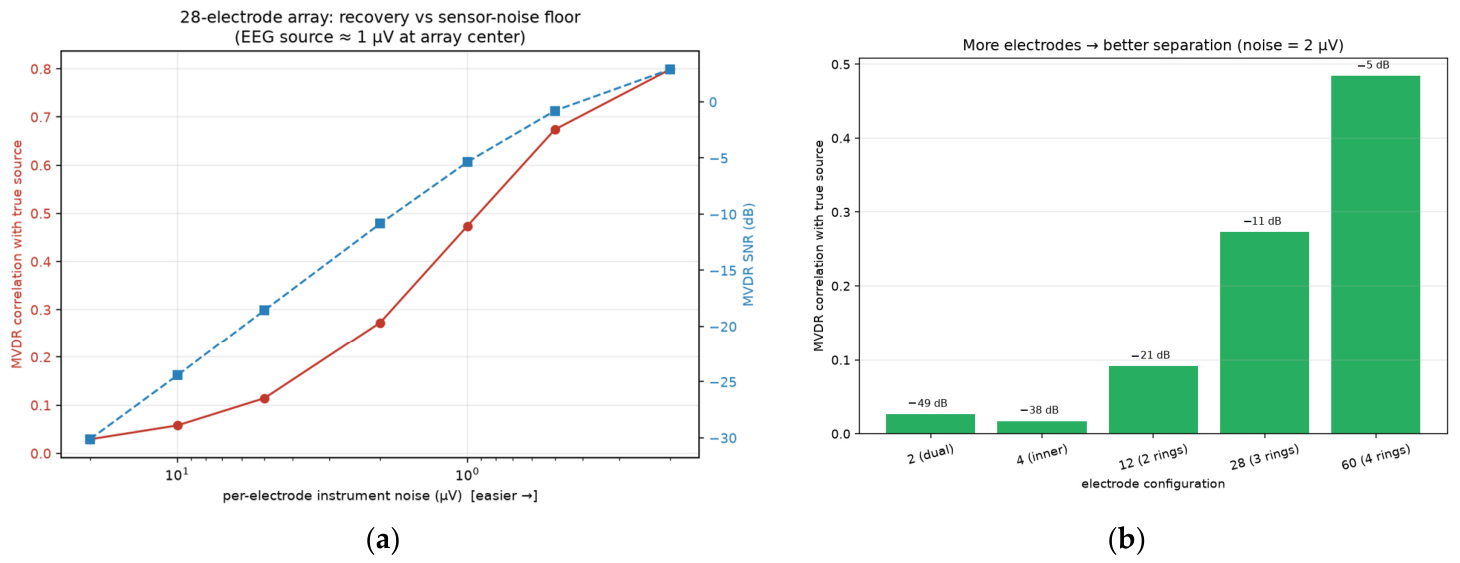
Two diagnostic sweeps show that the limiting factors are (1) independent per-electrode sensor noise and (2) the number of spatial degrees of freedom for nulling interference. Lowering noise from 20 µV to 0.2 µV raises correlation from ~0.03 to ~0.80 (Figure 17a); increasing from 2 to 60 electrodes raises correlation from ~0.03 to ~0.48 at fixed 2 µV noise (Figure 17b).
Figure 17.
Effect of different parameters on recovery performance: (a) sensor-noise floor and (b) number of electrodes.
3.6. Distributed Source Analysis
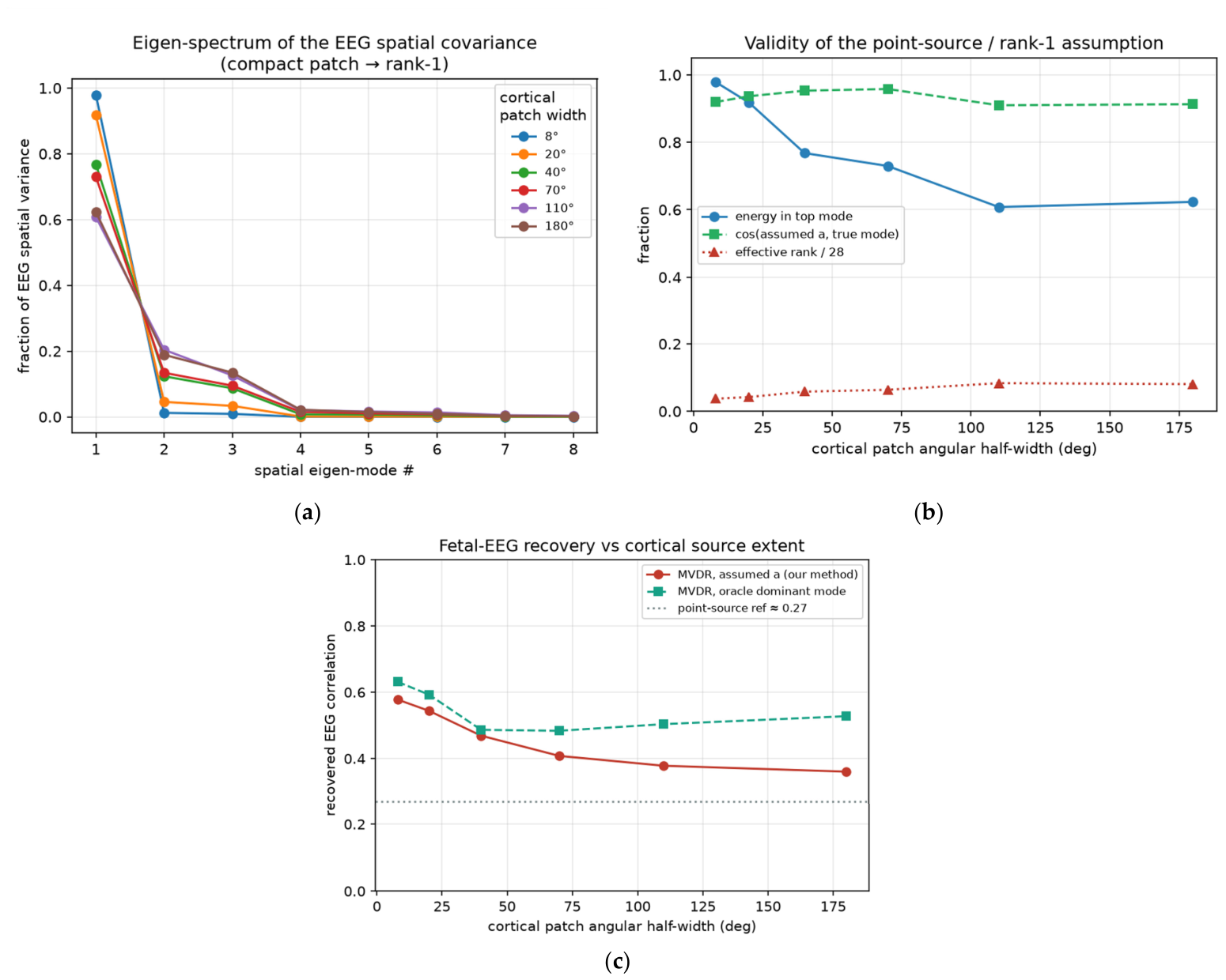
The current model treats the fetal EEG as a single point source. In reality, the EEG is the spatial integral of an enormous number of elementary generators, post-synaptic dendritic currents generated by large populations of cortical pyramidal neurons distributed across the folded fetal cortex [15,16]. This is the most important modeling caveat, so its impact was quantified. As depicted in Figure 18 the cortex was modeled as multiple independent radial current dipoles distributed on a spherical shell (representing the fetal scalp), summed their 1/r2 lead-fields at the 28 electrodes, and widened the active cortical patch from a near-point (8°) to the entire near hemisphere (180°). The following three questions were asked: (i) how diffuse or “spread out” is the resulting EEG across the array (effective rank)? (ii) does the assumed point-source steering vector still match the true dominant spatial pattern? and (iii) how much signal recovery is lost?
Figure 18.
Schematic representation of the distributed cortical source dipole model in the immature brain of a fetus.
Treating the fetal EEG as a distributed cortical integral (temporal-spatial summation of many dipoles projected over a spherical shell) does not invalidate the point-source steering vector: the abdominal array sees low effective rank (≈1–2) and the assumed steering vector a stays >0.9 aligned with the dominant spatial mode.
Table 3 summarizes the quantitative findings of the relevance estimation analysis.
Table 3.
Effect of cortical source extent on spatial structure and recovery (150 dipoles). Even a full-hemisphere source stays low-rank and well-aligned with the assumed steering vector.
- Low effective rank: the per-electrode EEG covariance has an effective rank of only 1.0–2.3 out of 28, because at a 10–12 cm standoff the array is in the far field of a ≤5 cm source, so many dipoles project onto the array almost collinearly;
- Dominant-mode energy: 61–98% of the EEG spatial variance lies in a single mode, with the highest values observed for compact sources and the lowest for a full hemisphere (Figure 19a);Figure 19. Distributed-source analysis. (a) the EEG spatial covariance is dominated by one eigen-mode (low rank). # indicates the index (order) of the eigenmode. (b) the assumed point-source steering vector stays 0.91–0.96 aligned with the true dominant mode for all source sizes. (c) recovery of the dominant EEG mode degrades only gracefully as the cortex spreads.
- Assumption stays valid: the assumed point-source steering vector a = (dmin/d)2 remains 0.91–0.96 cosine-aligned with the true dominant mode across all source extents, i.e., centering the array on the head captures the net cortical dipole regardless of how spread out the activity is (Figure 19b);
- Graceful degradation: MVDR using the assumed steering vector a recovers the dominant EEG mode with correlation 0.58 (compact) falling to 0.36 (whole hemisphere); an oracle that knew the true mode would only reach 0.63–0.48, so the point-source assumption itself costs little (Figure 19c);
- Genuine limitation: for widely distributed activity, a growing minority (up to ~40%) of EEG energy sits in higher spatial modes that a single-constraint beamformer cannot pass. This is the part a multi-beam/subspace (LCMV with multiple constraints, or GEVD) extension should target.
3.7. Real Neonatal EEG Validation
To test whether synthetic conclusions generalize, we replace the synthetic EEG generator with real scalp EEG from two public databases, OpenNeuro ds004577 and Zenodo 1280684, while retaining the same abdominal mixture model and 28-electrode geometry. This experiment evaluates whether the beamforming framework remains effective when realistic EEG waveforms are used as the underlying source. However, it does not validate the physical assumptions of the abdominal forward model, including the inverse-square attenuation (1/r2), the point-source approximation, or the spatial separability of real abdominal interferences, since the recordings are postnatal scalp EEGs rather than transabdominal fetal EEGs. Therefore, these experiments should be interpreted as a first-order validation of the signal recovery framework rather than a direct validation of the complete physiological model.
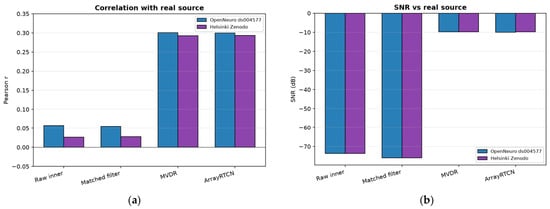
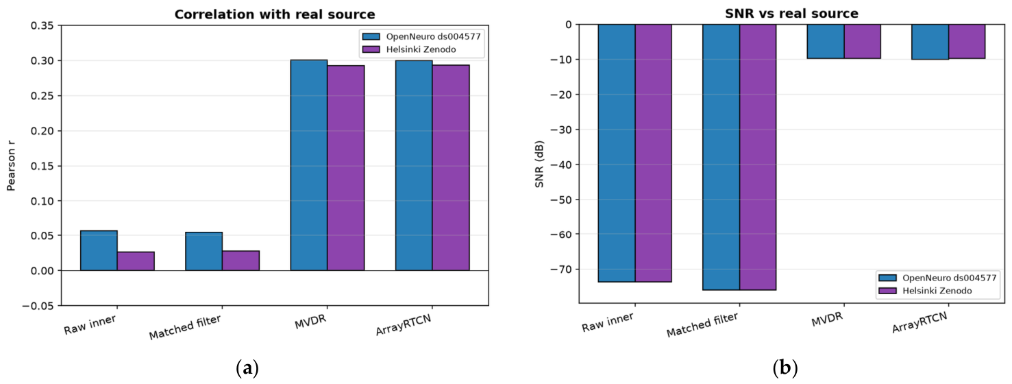
Table 4 and Table 5 summarize the recovery results on the OpenNeuro ds004577 and Helsinki Zenodo datasets. The raw inner electrode and matched filter yielded poor recovery, while the MVDR beamformer markedly improved the correlation coefficient and RMSE. ArrayRTCN achieved nearly identical performance to MVDR, and the consistent results across both datasets demonstrate the robustness of the proposed framework. Recording-level statistics on the same cached test windows confirm the effect: MVDR exceeds the matched filter and the raw inner electrode with p < 0.001 on both real-EEG datasets (OpenNeuro: window-mean r = 0.300, cluster-bootstrap 95% CI 0.286–0.316, 16 test segments/144 windows; Helsinki: window-mean r = 0.279, 95% CI 0.262–0.294, 16 test segments/144 windows). ArrayRTCN is statistically indistinguishable from MVDR (p = 0.87 OpenNeuro, p = 0.94 Helsinki). The synthetic test split has only two recordings, so its sign-flip p-value is floor-limited (~0.50) despite non-overlapping bootstrap CIs; we therefore report the CIs and do not claim a synthetic p-value (Figure 20).
Table 4.
Recovery on OpenNeuro ds004577 dataset.
Table 5.
Recovery on Helsinki Zenodo dataset.
Figure 20.
Recovery performance on real EEG datasets: (a) recovery correlation, (b) signal to noise ratio (SNR).
RMSE and SNR of the raw inner-electrode and matched-filter baselines are dominated by the shared synthetic abdominal interference and are therefore essentially identical across Table 4 and Table 5. Only the correlation coefficient, which depends on the injected EEG waveform, differs. Helsinki correlations in Table 5 are the window-level means on the cached test set.
3.8. Comparison with Synthetic Benchmark
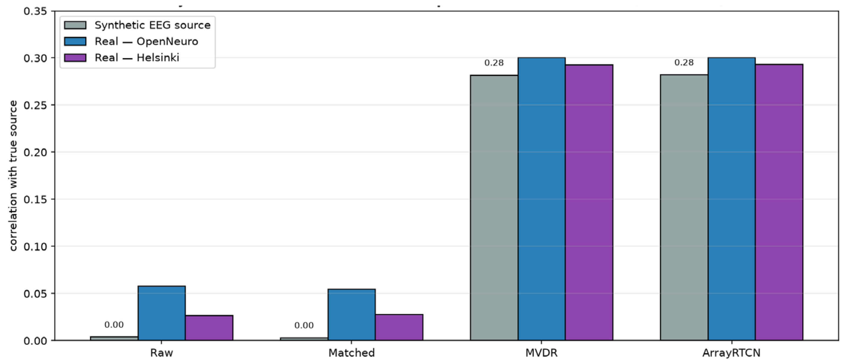
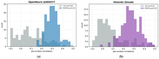
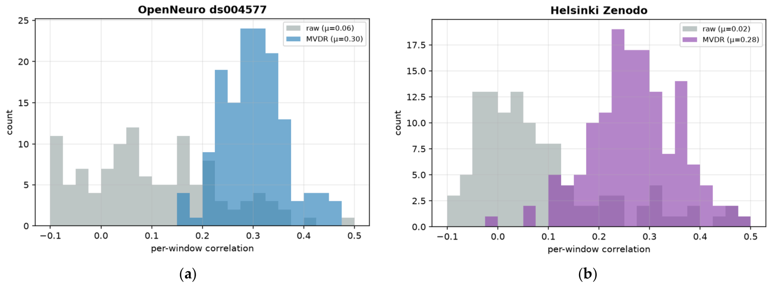
As displayed in Figure 21 the MVDR beamformer correlation on synthetic data matches OpenNeuro (0.300) and Helsinki (0.279). These consistent results suggest that the observed performance ceiling (r ≈ 0.29–0.30) is primarily determined by the linear mixing model and the 2 µV sensor noise, rather than by the simplicity of the synthetic EEG model. In contrast, the raw inner-electrode baseline consistently yielded negligible recovery (r ≈ 0.03–0.06, SNR ≈ −74 dB), confirming that effective spatial interference suppression, rather than simple coherent averaging, is essential for successful fetal EEG recovery (Figure 22).
Figure 21.
Synthetic versus real EEG source.
Figure 22.
Per-window MVDR correlation distribution on held-out real-data test windows: (a) OpenNeuro dataset. (b) Helsinki Zenodo dataset.
3.9. Robustness and Benchmarking Analyses
Multilayer volume conductor. An analytic five-layer concentric-sphere model (fetal brain to 4.3 cm; fetal skull to 4.75 cm; scalp to 5.0 cm; vernix caseosa to 5.15 cm; amniotic fluid to 7.0 cm; and maternal tissue as an unbounded 0.30 S/m medium) was solved for a radial dipole by Legendre expansion, with the solver validated against the closed-form homogeneous dipole (maximum relative error 10−11). The steering-vector shape is essentially preserved as follows: cosine similarity with the assumed 1/r2 vector is 0.997 for a central source and 0.988 for an eccentric superficial cortical source, and shape mismatch alone leaves MVDR recovery unchanged (r = 0.33 vs. 0.28 baseline). The decisive effect is absolute amplitude: the layered path passes 51% of the geometric prediction without vernix (−5.8 dB) but only 1.8% (≈−35 dB) through an intact 1.5 mm vernix layer, reducing recovery at the 2 µV noise floor from r = 0.18 to r = 0.01. Frequency-dependent tissue conductivity produces a negligible spectral tilt (−1.1 dB with vernix, −0.2 dB without, across 0.5–45 Hz). Gestational windows with absent or fissured vernix (before about 28 weeks and near term) are therefore the realistic operating regime, and the sub-microvolt noise-floor requirement of Section 3.5 becomes correspondingly stricter.
Geometric misalignment and head depth. With the beamformer holding the nominal steering vector, lateral head displacement up to 5 cm and array tilt up to 20° reduce the recovery correlation by less than 30% (r = 0.28 to 0.20 and 0.26, respectively), well within reported ultrasound placement accuracy. Depth misestimation is asymmetric: a head closer than assumed improves recovery (r = 0.56 at −3 cm), whereas overestimation degrades it (r = 0.15 at +3 cm). Sweeping the true depth from 6 to 14 cm shows that performance is governed by the physical 1/d2 amplitude at the electrodes (r = 0.71 at 6 cm; 0.13 with a known steering vector and 0.12 with the assumed 10 cm vector at 14 cm): per-electrode SNR, not steering mismatch, is the limiting factor.
Electrode-impedance drift. Modulating each electrode’s physiological content by a slow Ornstein–Uhlenbeck gain process (time constant 8 s) collapses MVDR recovery from r = 0.29 to r = 0.06 at only 5% gain-drift standard deviation, and to chance level at 10%; per-window covariance re-estimation outperforms a whole-recording covariance but cannot rescue performance. The mechanism is fundamental: nulling a ~10 mV maternal ECG to below a 1 µV target requires the relative, channel-to-channel gain of the complete acquisition chain (electrode–skin interface, analog front-end, and any subsequent digital scaling) to remain stable to order 10−4 after calibration. This is not a specification on the absolute amplifier gain of a single channel. A 5% inter-electrode gain-drift standard deviation already collapses MVDR from r = 0.29 to r = 0.06. Modern EEG front-ends routinely achieve sub-0.1% absolute gain accuracy, but the 10−4 relative requirement is tighter than uncompensated electrode–skin impedance drift; it is realistic only with active impedance monitoring, frequent recalibration, and/or robust adaptive beamforming. This non-stationary regime is the realistic arena in which the learned ArrayRTCN branch could add value beyond a linear beamformer, and it is not claimed as a present performance contribution.
Statistics and comparison with existing method families. Recording-level cluster-bootstrap confidence intervals and paired sign-flip permutation tests were added for all test sets; MVDR exceeds the matched filter and the raw inner electrode at p < 0.001 on both real-EEG datasets, and ArrayRTCN is statistically indistinguishable from MVDR (p = 0.87 and 0.94). On identical synthetic test windows, classical families fail at the ~100 dB interference-to-signal ratio of the 1 µV problem even when granted oracle information: PCA r = 0.008, oracle-selected FastICA r = 0.021, least-squares adaptive cancelation r = −0.005, and oracle-noise-covariance GEVD multichannel Wiener filtering is unstable (r = −0.038 ± 0.33), whereas MVDR attains r = 0.279. The known geometric steering vector of the concentric array, not generic source separation, is the decisive prior. Methods developed for the roughly 100-fold larger fetal-ECG problem do not transfer. Random gains in [0.6, 1.4] already have high cosine similarity with a (mean 0.97) because both vectors lie in the positive orthant; MVDR nevertheless attains r = 0.28 by exploiting the residual angular difference. Interpolating those gains onto itself collapses recovery to chance (r = 0.009). Spatial separability is therefore necessary, and in this study, it is imposed by construction.
Biomarker-level recovery. Although sample-level correlation is r ≈ 0.3, clinically oriented aggregate features survive substantially better: aEEG-style amplitude envelopes correlate at 0.40–0.62 with the true source across the three test sets, band-power trends reach 0.72 (theta), and a simple burst detector transfers with about 0.5 sensitivity at 0.35–0.75 precision. Envelope- and trend-level monitoring is thus a plausible target for future translational evaluation, while waveform-level interpretation remains beyond the current recovery quality.
4. Discussion
The decisive architectural change is the concentric array with known geometry: it converts the fetal EEG into a rank-1 source with a computable steering vector, enabling MVDR to place spatial nulls on high-variance interferers. Dual-electrode subtraction improves SNR but lacks sufficient spatial degrees of freedom. Recovery is ultimately limited by independent per-electrode noise; synthetic sweeps show correlation rising from ~0.03 to ~0.80 when noise falls from 20 µV to 0.2 µV.
Real neonatal validation strengthens the feasibility argument as follows: broadband, non-stationary real waveforms, including NICU recordings with seizure activity, are recovered at the same correlation level as idealized synthetic bursts. Remaining gaps include real abdominal interference (whose spatial profile is not known to be distinct from the fetal EEG), fetal movement, and genuine transabdominal recordings. Exploratory band-power and burst endpoints are now reported in Section 3.9 and should not be read as clinical validation.
The revision analyses sharpen this picture. The multilayer volume-conductor study shows that the geometric steering assumption is benign but that an intact vernix caseosa can cost ≈35 dB of amplitude. Consequently, the headline r ≈ 0.28, obtained under a homogeneous 1/r2 model with a 1 µV abdominal target, should not be interpreted as expected performance under all in vivo conditions: feasibility depends strongly on gestational age and vernix state, and the required sensor noise floor becomes considerably more stringent when that attenuation is included. The impedance-drift study adds a relative, post-calibration, channel-to-channel gain-stability requirement of order 10−4 for deep interference nulling. The biomarker analysis indicates that envelope- and band-power-level monitoring, rather than waveform reading, is a plausible target for future translational evaluation. The statistical results are recording- or segment-level feasibility evidence from six source recordings per neonatal corpus (16 held-out test segments), not population-level clinical evidence. Finally, except for the alignment sweep, spatial separability of fetal EEG from maternal ECG is imposed by the synthetic generator; it has not been demonstrated on abdominal recordings. These results reinforce that the present contribution is engineering feasibility of the spatial-recovery principle, with clinical validation contingent on hardware noise, impedance stability, gestational-age-dependent attenuation, and in vivo confirmation.
4.1. Future Work
4.1.1. Hardware and Array Design
- Minimizing per-electrode input-referred noise using high-fidelity EEG amplifiers and ultra-sensitive electrodes is the single most effective strategy for improving signal recovery performance;
- Increase the number of rings/electrodes to add interference-nulling degrees of freedom;
- Maintain accurate array centering via repetitive ultrasound tracking of the head center position.
4.1.2. Modeling Fidelity
- Replace the analytic five-layer sphere of Section 3.9 with a subject-specific FEM/BEM forward model of non-spherical maternal anatomy, fetal position, and vernix state;
- Add inter-electrode propagation delays (convolutive, not instantaneous, mixing); frequency-dependent conductivity was already found to produce negligible 0.5–45 Hz tilt in Section 3.9;
- Model fetal movement and resulting steering-vector mismatch; evaluate robust/adaptive beamformers (diagonal-loading, worst-case-optimal);
- Introduce 50/60 Hz mains and electrode pop/detachment; electrode-impedance drift is quantified in Section 3.9 and remains a hardware requirement rather than an open modeling question;
- Add nonlinear and non-stationary interference so the neural network can demonstrate value beyond the linear beamformer.
4.1.3. Algorithms and Validation
- Jointly cancel maternal and fetal ECG using their (estimable) cardiac timing as auxiliary information;
- Explore space-time beamforming; oracle GEVD/Wiener and FastICA baselines are already reported in Section 3.9 and do not recover the 1 µV source;
- Validate on actual abdominally acquired fetal EEG recordings, ideally with a reference fetal scalp electrode when ethically available;
- Validate exploratory envelope and burst endpoints on true transabdominal recordings rather than on injected neonatal EEG.
As concrete next steps, we commit to: (i) subject-specific FEM/BEM forward models of the maternal abdomen (non-spherical anatomy, fetal position, gestational-age-dependent vernix state), extending the analytic multilayer analysis of Section 3.9; and (ii) a staged in vivo program consisting of physical phantom validation followed by transabdominal recordings with simultaneous ultrasound localization of the fetal head.
5. Conclusions
Using synthetic data, a single abdominal electrode cannot recover the ~1 µV fetal EEG (correlation ~0). It is buried ~80 dB below ambient electronic noise from sources such as the maternal ECG and exceeded by every other source including electrode sensor noise.
A dual electrode with a subtraction network improves SNR (~+27 dB) but still does not reach waveform-level correlation.
A concentric 28-electrode array centered over the fetal head makes the EEG a rank-1 source with a known attenuation steering vector. An MVDR beamformer exploiting that vector raises correlation from ~0 to ~0.28 and SNR by ~67 dB, a decisive architectural change.
The physical intuition behind the array design is confirmed (outer rings see weaker EEG), with inverse-square (1/d2) attenuation; the across-ring gradient is real but modest (0.94 -> 0.64) because the 10 cm depth dominates the ring radii.
The learned ArrayRTCN matches but does not beat MVDR, as expected for a linear mixture where the optimal linear filter is near-optimal overall. We therefore reposition the learned branch as a scaffold for future non-stationary operating conditions (e.g., the electrode-impedance drift regime of Section 3.9, where linear beamforming degrades sharply) rather than as a present performance contribution.
Signal recovery is ultimately limited by independent per-electrode noise and the available spatial degrees of freedom. Both can be improved by hardware and array design.
Treating the fetal EEG as a distributed source (the integral of many cortical dipoles) does not break the approach. The EEG remains low-rank as seen from the abdomen (effective rank ~1–2), and the assumed point-source steering vector stays >0.9 aligned with the true dominant mode, so the array recovers the dominant cortical activity component represented within the simulated forward model. No fetal hypoxia cohort and no genuine transabdominal fetal EEG recordings were evaluated.
Author Contributions
Conceptualization: A.G. and O.E.; methodology: A.N., N.M., H.G., R.C., and A.G.; software: A.N., N.M., H.G., and A.G.; validation: A.N., A.G., O.E., R.C., and E.S.; formal analysis: A.N., A.G., H.G., R.C., and N.M.; investigation: A.N., N.M., H.G., R.C., and A.G.; resources: A.G.; data curation: R.C., O.E., and E.S.; writing—original draft preparation: A.N., A.G., and R.C.; writing—review and editing: A.N., A.G., R.C., O.E., and E.S.; visualization: A.N., A.G., R.C., and O.E.; supervision: A.G. and O.E.; project administration: A.G.; funding acquisition: A.G. and O.E. All authors have read and agreed to the published version of the manuscript.
Funding
This research was funded by the Ministry of Innovation, Science and Technology, Israel; grant number 0004750.
Institutional Review Board Statement
This study used a synthetic abdominal mixture model and publicly available de-identified neonatal EEG (OpenNeuro ds004577 and Zenodo 1280684). No new human-subject recordings were acquired by the authors for the analyses reported here; institutional review board approval was not required.
Informed Consent Statement
Not applicable. The public datasets were released under their original ethical approvals; no additional consent was obtained for this secondary analysis.
Data Availability Statement
The OpenNeuro ds004577 infant EEG dataset is publicly available at https://openneuro.org/datasets/ds004577. Accessed on 12 April 2026. The Helsinki neonatal EEG corpus is available from Zenodo (record 1280684). Synthetic mixture code and the revision experiments are archived in ConcentricFetalEEG.v2.
Conflicts of Interest
Authors Ali Nasirlou, Niki Manouchehri, and Helen Guez were employed by the company FetalEEG Inc. The remaining authors declare that the research was conducted in the absence of any commercial or financial relationships that could be construed as a potential conflict of interest The funders had no role in the design of the study; in the collection, analyses, or interpretation of data; in the writing of the manuscript; or in the decision to publish the results.
Appendix A. Experimental Configuration
- Electrodes: 28 (rings [4, 8, 16], radii [2.5, 5.0, 7.5] cm);
- Head: radius 5.0 cm, center depth 10.0 cm; attenuation power p = 2.0;
- Recordings: 16 × 20.0 s; windows [“train”: 108, “val”: 18, “test”: 18];
- Training: 25 epochs, batch 16, lr 0.002, sensor noise 2.0 µV.
Appendix B. Algorithm Reference (Signal-Flow Graphs and Derivations)
Every method that produces a number in this report is documented below with a signal-flow graph, the governing equations, a step-by-step explanation, and its strengths and limitations. Common notation: x(t) ∈ ℝE is the vector of E electrode samples at time t; a ∈ ℝE is the known geometric attenuation steering vector (ak = (dmin/dk)2); s(t) is the fetal-EEG source; and n(t) lumps all interference + sensor noise. All methods operate on per-window, MAD-normalized data.
Appendix B.1. Shared Preprocessing
- Windowing: signals are cut into 4 s windows (4000 samples at fs = 1000 Hz) with 50% overlap;
- Robust normalization: each window is divided by a median-absolute-deviation (MAD) scale, scale = 1.4826·median(|x − median(x)|), which is robust to the large maternal-ECG spikes; the scale is stored so estimates can be returned to physical units (volts/µV);
- Splitting: train/validation/test partitions are by recording seed, preventing window leakage.
Appendix B.2. Algorithm A: Single/Raw Electrode Baseline
Purpose: A lower bound representing what a conventional single abdominal lead sees.
How it works: The electrode with the largest attenuation (the inner-ring electrode k* = argmax ak, i.e., closest to the head) is selected and divided by its known attenuation to express the estimate at the source scale (Figure A1)
Why it fails: Since
and the interferers are up to ~10 mV versus the ~1 µV EEG, the output is overwhelmingly interference: correlation with the true EEG ≈ 0, SNR ≈ −77 dB. No cancelation is performed.
Figure A1.
Signal-flow graph of the single-electrode baseline.

Appendix B.3. Algorithm B: Matched-Filter (Least-Squares) Estimator
Model: x(t) = a·s(t) + n(t), treating everything but the EEG as additive noise n [26].
Derivation: Minimizing the squared error ‖x − a·s‖2 over the scalar s gives the closed-form least-squares (matched-filter) solution
This is the maximum-likelihood estimate when n is spatially white and Gaussian.
How it works and limitation: It coherently sums the electrodes weighted by their expected EEG amplitude, giving a √-type SNR gain against spatially white noise. However, it does not account for the spatial structure of the interference, so the large, spatially correlated maternal ECG is only averaged, not nulled. Result here: correlation ≈ 0, SNR ≈ −77 dB.
Figure A2.
Signal-flow graph of the matched-filter/least-squares estimator. Optimal for white noise; passes a at unit gain but does not null structured interference.
Appendix B.4. Algorithm C: MVDR/LCMV Beamformer
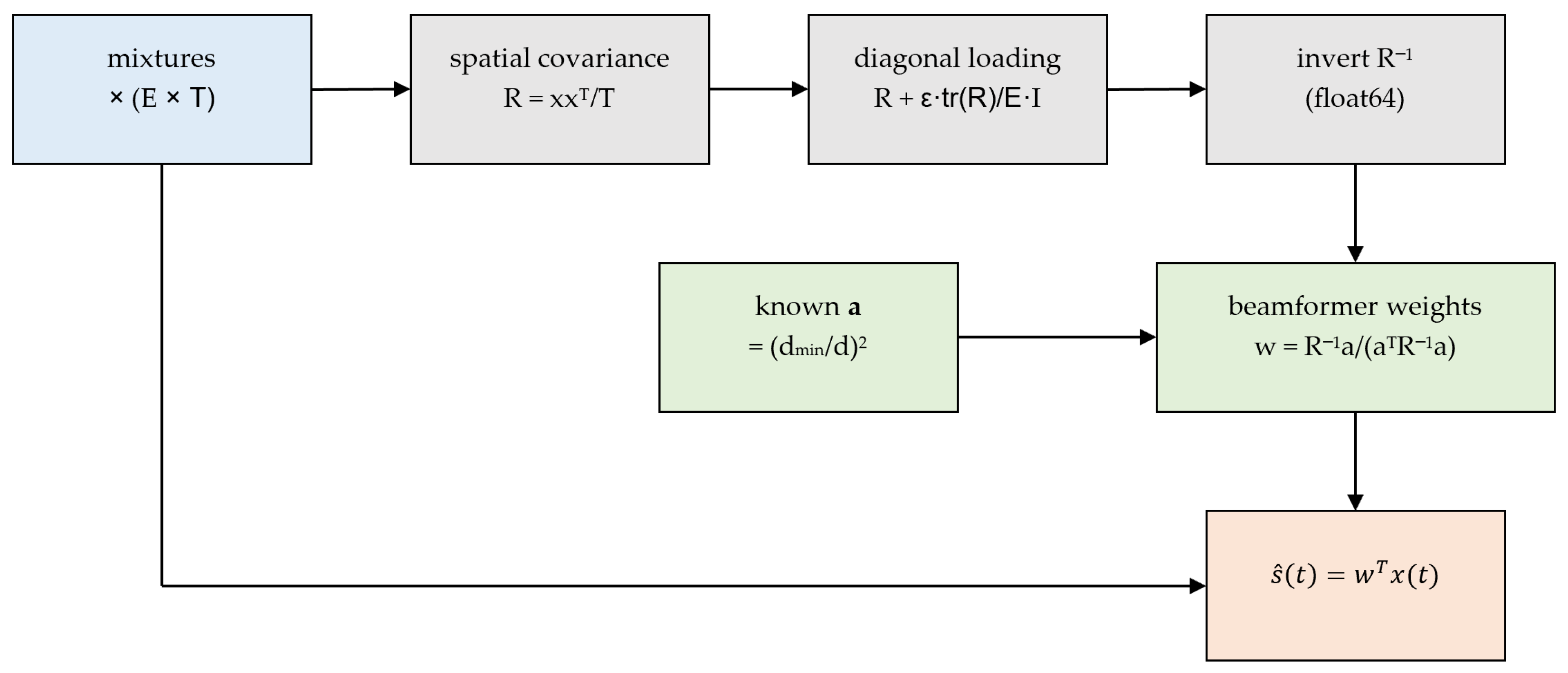
Objective (minimum-variance distortionless response): Find spatial weights w that minimize total output power while passing the EEG direction undistorted: minimize wᵀRw subject to wᵀa = 1, where R = E[x xᵀ] is the spatial covariance [14].
Closed-form solution:
Step-by-step (Figure A3):
- Estimate the E × E spatial covariance from the window: R = x xᵀ/T;
- Apply diagonal loading R ← R + ε · tr(R)/E · I (ε = 1 × 10⁻⁶) for numerical conditioning and robustness to steering-vector mismatch [27];
- Invert R in float64, essential because the maternal-ECG/EEG dynamic range gives R a condition number of 106–1012; float32 inversion is uns and was the original failure mode.
- Form the weights w = R−1a/(aᵀR−1a) and apply ŝ = wᵀx.
Why it works: The distortionless constraint guarantees unit gain on the EEG direction a, while minimizing output variance forces the weights to place spatial nulls on the high-power interferers. Because each interferer’s spatial gain vector differs from a, with E = 28 electrodes the beamformer can null up to 27 interfering directions and still pass the EEG. This is the decisive step: correlation rises from ≈0 to ≈0.28 and SNR by ≈67 dB.
Figure A3.
Signal-flow graph of the MVDR/LCMV beamformer (exploits the known steering vector a).
Appendix B.5. Algorithm D: DualRTCN (Dual-Electrode Subtraction Network)
Architecture (Figure A4):
- Input: the two-channel normalized mixture (2 × T);
- Input 1-D convolution (kernel 7) lifting to 48 feature channels;
- Eight dilated residual blocks (two Conv1d layers each, GroupNorm + GELU, dilations 1, 2, 4, …, 128) giving a wide temporal receptive field (~hundreds of ms) [28];
- A 1 × 1 convolution head predicting the shared interference on channel 1, î_interf(t);
- Subtraction: (t) = xch1(t) − îinterf(t).
Training: Targets are the true interference and EEG on channel 1; loss = L1() + L1(îinterf) + 0.5·multi-resolution-STFT-L1, optimized with Adam [29].
Rationale and limitation: It is easier to model the strong, structured interference than the weak EEG directly, so the network predicts and subtracts it (Conv-TasNet/fetal-ECG-cancelation style) [28]. With only two channels there is little spatial diversity and no known geometric model, so it improves SNR (~+27 dB) but does not reach waveform-level correlation.
Figure A4.
Signal-flow graph of the DualRTCN subtraction network.

Appendix B.6. Algorithm E: ArrayRTCN (Physics-Informed Array Network)
Architecture (Figure A5):
- Physics front-end: from the 28-channel input and the known a buffer, compute the matched-filter estimate sls = aᵀx/(aᵀa) and the batched MVDR estimate smvdr (in float64, detached from the gradient);
- Concatenate [x (28), sls, smvdr] → 30 input channels;
- Input Conv (kernel 7 → 48 ch) followed by the same eight dilated residual blocks;
- A zero-initialized 1 × 1 correction head; output = smvdr + correction.
Training: Target is the EEG source; loss = L1 + 0.5·MR-STFT-L1 (Adam). Because the correction head is zero-initialized, the network starts exactly at the MVDR estimate and only learns a residual refinement.
Rationale and finding: Handing the network the optimal linear (MVDR) solution as a physics prior removes the burden of re-learning beamforming and stabilizes training. In this linear-mixture regime it matches MVDR (correlation ≈ 0.28); its value would emerge against nonlinear or non-stationary interference, where a fixed linear beamformer is sub-optimal.
Figure A5.
Signal-flow graph of the physics-informed ArrayRTCN.
References
- Castel, A.; Frank, Y.S.; Feltner, J.; Karp, F.B.; Albright, C.M.; Frasch, M.G. Monitoring Fetal Electroencephalogram Intrapartum: A Systematic Literature Review. Front. Pediatr. 2020, 8, 584. [Google Scholar] [CrossRef] [Scilit] [PubMed]
- Je, L. 4 Million Neonatal Deaths: When? Where? Why? Lancet 2005, 365, 891–900. [Google Scholar] [CrossRef] [Scilit] [PubMed]
- Finn, D.; Dempsey, E.M.; Boylan, G.B. Lost in Transition: A Systematic Review of Neonatal Electroencephalography in the Delivery Room—Are We Forgetting an Important Biomarker for Newborn Brain Health? Front. Pediatr. 2017, 5, 173. [Google Scholar] [CrossRef] [Scilit] [PubMed]
- André, M.; Lamblin, M.-D.; d’Allest, A.-M.; Curzi-Dascalova, L.; Moussalli-Salefranque, F.; Tich, S.N.T.; Vecchierini-Blineau, M.-F.; Wallois, F.; Walls-Esquivel, E.; Plouin, P. Electroencephalography in Premature and Full-Term Infants. Developmental Features and Glossary. Neurophysiol. Clin./Clin. Neurophysiol. 2010, 40, 59–124. [Google Scholar] [CrossRef] [Scilit] [PubMed]
- Awal, M.A.; Lai, M.M.; Azemi, G.; Boashash, B.; Colditz, P.B. EEG Background Features That Predict Outcome in Term Neonates with Hypoxic Ischaemic Encephalopathy: A Structured Review. Clin. Neurophysiol. 2016, 127, 285–296. [Google Scholar] [CrossRef] [Scilit] [PubMed]
- Thaler, I.; Boldes, R.; Timor-Tritsch, I. Real-Time Spectral Analysis of the Fetal EEG: A New Approach to Monitoring Sleep States and Fetal Condition During Labor. Pediatr. Res. 2000, 48, 340–345. [Google Scholar] [CrossRef] [Scilit] [PubMed]
- Djelmis, J.; Dražančić, A.; Dürrigl, V.; Ivanšenić, M. The Effect of Fetal Hypoxia and Acidosis on the Changes in Fetal Electroencephalogram During Labor. Am. J. Perinatol. 1988, 5, 177–185. [Google Scholar] [CrossRef] [Scilit] [PubMed]
- Chock, V.Y.; Rao, A.; Van Meurs, K.P. Optimal Neuromonitoring Techniques in Neonates with Hypoxic Ischemic Encephalopathy. Front. Pediatr. 2023, 11, 1138062. [Google Scholar] [CrossRef] [Scilit] [PubMed]
- Bonifacio, S.L.; Glass, H.C.; Peloquin, S.; Ferriero, D.M. A New Neurological Focus in Neonatal Intensive Care. Nat. Rev. Neurol. 2011, 7, 485–494. [Google Scholar] [CrossRef] [Scilit] [PubMed]
- Chang, T.; Tsuchida, T.N. Conventional (Continuous) EEG Monitoring in the NICU. Curr. Pediatr. Rev. 2014, 10, 2–10. [Google Scholar] [CrossRef] [Scilit] [PubMed]
- Tsuchida, T.N.; Wusthoff, C.J.; Shellhaas, R.A.; Abend, N.S.; Hahn, C.D.; Sullivan, J.E.; Nguyen, S.; Weinstein, S.; Scher, M.S.; Riviello, J.J.; et al. American Clinical Neurophysiology Society Standardized EEG Terminology and Categorization for the Description of Continuous EEG Monitoring in Neonates: Report of the American Clinical Neurophysiology Society Critical Care Monitoring Committee. J. Clin. Neurophysiol. 2013, 30, 161–173. [Google Scholar] [CrossRef] [Scilit] [PubMed]
- Shao, M.; Barner, K.E.; Goodman, M.H. An Interference Cancellation Algorithm for Noninvasive Extraction of Transabdominal Fetal Electroencephalogram (TaFEEG). IEEE Trans. Biomed. Eng. 2004, 51, 471–483. [Google Scholar] [CrossRef] [Scilit] [PubMed]
- Sulas, E.; Urru, M.; Tumbarello, R.; Raffo, L.; Pani, D. Systematic Analysis of Single-and Multi-Reference Adaptive Filters for Non-Invasive Fetal Electrocardiography. Math. Biosci. Eng. 2020, 17, 286–308. [Google Scholar] [CrossRef] [Scilit] [PubMed]
- Van Veen, B.D.; Buckley, K.M. Beamforming: A Versatile Approach to Spatial Filtering. IEEE ASSP Mag. 1988, 5, 4–24. [Google Scholar] [CrossRef] [Scilit] [PubMed]
- Nunez, P.L.; Srinivasan, R. Electric Fields of the Brain: The Neurophysics of EEG; Oxford University Press: Oxford, UK, 2006. [Google Scholar]
- Sarvas, J. Basic Mathematical and Electromagnetic Concepts of the Biomagnetic Inverse Problem. Phys. Med. Biol. 1987, 32, 11–22. [Google Scholar] [CrossRef] [Scilit] [PubMed]
- Ebersole, J.S.; Pedley, T.A. Current Practice of Clinical Electroencephalography; Lippincott Williams & Wilkins: Philadelphia, PA, USA, 2003. [Google Scholar]
- Wolters, C.H.; Anwander, A.; Tricoche, X.; Weinstein, D.; Koch, M.A.; Macleod, R.S. Influence of Tissue Conductivity Anisotropy on EEG/MEG Field and Return Current Computation in a Realistic Head Model: A Simulation and Visualization Study Using High-Resolution Finite Element Modeling. NeuroImage 2006, 30, 813–826. [Google Scholar] [CrossRef] [Scilit] [PubMed]
- Sameni, R. Noninvasive Fetal Electrocardiography: Models, Technologies, and Algorithms. In Innovative Technologies and Signal Processing in Perinatal Medicine: Volume 1; Springer: Cham, Switzerland, 2020; pp. 99–146. [Google Scholar]
- Xiao, Y.; Yin, J.; Qi, H.; Yin, H.; Hua, G. MVDR Algorithm Based on Estimated Diagonal Loading for Beamforming. Math. Probl. Eng. 2017, 2017, 7904356. [Google Scholar] [CrossRef] [Scilit]
- Bai, S.; Kolter, J.Z.; Koltun, V. An Empirical Evaluation of Generic Convolutional and Recurrent Networks for Sequence Modeling. arXiv 2018, arXiv:1803.01271. [Google Scholar]
- He, K.; Zhang, X.; Ren, S.; Sun, J. Deep Residual Learning for Image Recognition. In Proceedings of the IEEE Conference on Computer Vision and Pattern Recognition, Las Vegas, NV, USA, 27–30 June 2016. [Google Scholar]
- Harmony, T.; Otero-Ojeda, G.; Aubert, E.; Fernández, T.; Cubero-Rego, L. Dataset Containing Resting Eeg for a Sample of 103 Normal Infants in the First Year of Life. 2023, OpenNeuro. org. Available online: https://openneuro.org/datasets/ds004577/versions/1.0.1 (accessed on 12 April 2026).
- Harmony, T.; Otero-Ojeda, G.; Aubert-Vázquez, E.; Fernández, T.; Cubero-Rego, L. Normative Longitudinal Eeg Recordings During Sleep Stage Ii in the First Year of Age. Sci. Data 2024, 11, 784. [Google Scholar] [CrossRef] [Scilit] [PubMed]
- Stevenson, N.J.; Tapani, K.; Lauronen, L.; Vanhatalo, S. A Dataset of Neonatal Eeg Recordings with Seizure Annotations. Sci. Data 2019, 6, 190039. [Google Scholar] [CrossRef] [Scilit] [PubMed]
- Van Trees, H.L. Optimum Array Processing: Part IV of Detection, Estimation, and Modulation Theory; John Wiley & Sons: Hoboken, NJ, USA, 2002. [Google Scholar]
- Stoica, P.; Wang, Z.; Li, J. Robust Capon Beamforming. In Proceedings of the Conference Record of the Thirty-Sixth Asilomar Conference on Signals, Systems and Computers, 2002, Pacific Grove, CA, USA, 3–6 November 2002. [Google Scholar]
- Luo, Y.; Mesgarani, N. Conv-Tasnet: Surpassing Ideal Time–Frequency Magnitude Masking for Speech Separation. IEEE/ACM Trans. Audio Speech Lang. Process. 2019, 27, 1256–1266. [Google Scholar] [CrossRef] [Scilit] [PubMed]
- Yamamoto, R.; Song, E.; Kim, J.-M. Parallel WaveGAN: A Fast Waveform Generation Model Based on Generative Adversarial Networks with Multi-Resolution Spectrogram. In Proceedings of the ICASSP 2020–2020 IEEE International Conference on Acoustics, Speech and Signal Processing (ICASSP), Barcelona, Spain, 4–8 May 2020. [Google Scholar]



Disclaimer/Publisher’s Note: The statements, opinions and data contained in all publications are solely those of the individual author(s) and contributor(s) and not of MDPI and/or the editor(s). MDPI and/or the editor(s) disclaim responsibility for any injury to people or property resulting from any ideas, methods, instructions or products referred to in the content. |
© 2026 by the authors. Licensee MDPI, Basel, Switzerland. This article is an open access article distributed under the terms and conditions of the Creative Commons Attribution (CC BY) license.