


Abstract
Operator diagnosis level in a main control room (MCR) of Nuclear Power Plants (NPPs) is a core factor in preventing human errors and ensuring the safe operation of NPPs. Due to the high uncertainty of human behaviors and the scarcity of relevant data, traditional analysis methods mainly rely on empirical judgment, which suffer from insufficient dynamics and poor engineering adaptability. To address the issues, this paper conducts a study on an AI prediction model for operator diagnosis level in a MCR of NPPs based on the SACADA database and machine learning technology. The model adopts a probabilistic neural network (PNN) as the main architecture, and proposes a hybrid method of network search considering density distribution combined with K-fold cross-validation, which breaks the traditional mode of a single smoothing factor adapting to an entire dataset. The analysis results show that the performance of the hybrid method proposed in this paper outperforms network search + K-fold cross-validation and particle swarm optimization + K-fold cross-validation methods in terms of accuracy, precision, recall, and F1-score. The five-fold cross-validation verifies that the model has good stability and good generalization ability. Further, the model is compared with common AI models such as BP neural network and RBF neural network. The results demonstrate that the proposed model has advantages in core indicators including overall accuracy (0.9444), macro-precision (0.9783), macro-recall (0.9063), and macro-F1-score (0.9362), and can effectively solve the problems of insufficient recognition of minority-class samples, overfitting, and underfitting. This research achieves professional and in-depth application of the SACADA database for diagnosis level prediction, extends existing research on prediction tasks, and delivers valuable theoretical insights and practical application significance.
1. Introduction
1.1. Research Background and Significance
The MCR of a Nuclear Power Plant (NPP) undertakes key functions such as parameter monitoring, anomaly identification, fault diagnosis, and emergency disposal. The diagnosis process is a critical part of operation and accident response. Operator diagnosis level, covering anomaly identification, fault location, hidden danger identification and other dimensions, directly determines the NPP’s ability to respond to various risks, serving as an important barrier to prevent operator errors and accidents. Existing studies show that human accidents account for 60–90% of NPP accidents [1]. To reduce human accidents, human reliability analysis methods have been developed, including the decision-making cognitive model [2], unsafe behavior classification method [3], and generalized linear mixed-effects model [4]. It can be seen that developing appropriate analysis methods is crucial to ensure the safe operation of NPPs and reduce human accidents, while human reliability is the core of preventing human errors, and the diagnosis process is a key link in reducing human accidents. However, limited by the scarcity of human error data, the current evaluation and prediction of human diagnosis level in NPPs still rely mainly on empirical judgment. Existing studies mostly focus on the prediction of error probability, with obvious limitations: first, traditional evaluation methods highly depend on expert judgment, which is subjective and inefficient, making it difficult to comprehensively and dynamically reflect the operators’ diagnosis level under different working conditions; second, the complex and variable operation conditions of NPPs, as well as the suddenness and uncertainty of various abnormal conditions and faults, have put forward higher requirements for the real-time performance and accuracy of operator diagnosis level, and traditional evaluation methods can no longer adapt to the digital and intelligent development needs of NPPs.
Against this background, constructing a data-driven prediction model for operator diagnosis level has become an urgent issue to be solved. Based on this, this study relies on the SACADA database and integrates artificial intelligence technology to build a scientific and efficient prediction model for operator diagnosis level in a MCR of NPPs. This research has important theoretical and practical significance: (1) Theoretically, it enriches the theoretical and methodological system of data-driven human reliability evaluation, effectively solves the core problem of objectively predicting operator diagnosis level under the scarcity of human error data, and promotes the transformation of human reliability analysis from experience-driven to data-driven and intelligence-driven; (2) practically, it can accurately predict operator diagnosis level, identify weak links and potential operator risks in the diagnosis process, provide scientific support for human error prevention and control, personalized training plans formulated by management, thereby improving the emergency disposal capacity of NPPs and ensuring the safe and stable operation of units. Its main innovation lies in realizing the deep integration of data and artificial intelligence technology, promoting the precise implementation of research results in actual safety management, advancing the research process of dynamic prediction of operator diagnosis level, and providing new ideas and technical support for human reliability research in the nuclear power industry.
1.2. Literature Review
Diagnosis reliability refers to the consistency, accuracy, and robustness of operators in identifying, interpreting, and responding to system anomalies or faults [5]. Through literature review, it is found that there are few research results on diagnosis reliability. This paper mainly reviews the current situation from three aspects: theoretical framework, methodological evolution, and application scenarios:
(1) Theoretical basis: Multiple studies show that several important influencing factors have a significant impact on diagnosis reliability, such as Fatigue [6], Workload and Stress [7], Situational Awareness [8], Human-System Interface (HSI) Design [9], Training and Experience [10]. The cooperative model proposed by Salas et al. points out that effective crew diagnosis relies on key elements such as psychological safety, mental models and mutual trust [11]. In 2015, Eisele verified the predictive validity of the Swedish Diagnosis Survey through structural equation modeling and found a significant correlation between diagnosis level satisfaction and performance influencing factors [12]. Chan clarified the necessity of multi-level analysis and emphasized the strict distinction between individual and crew level research dimensions [13]. Aiming at the diagnostic error probability of operators in advanced MCRs of NPPs, Jung et al. constructed a time-reliability correlation model to estimate human diagnostic error rates in digital human–machine interface environments [14]. Ringstad et al. pointed out that effective diagnosis needs to integrate a multi-dimensional evaluation framework covering core elements such as personnel competence, process efficiency, equipment status, and safety culture [15]. Morgan et al. proposed the Plan, Execute, Check, Act cycle, providing a structured path for iterative improvement of human diagnosis [16]. Chang et al. [17,18,19] published three research papers on the IDAC model, which took the lead in clarifying the core concepts and theoretical system in the information processing process. In 2023, aiming at decision-making errors in digital NPPs, Zhang et al. proposed a decision-making cognitive model and a classification system for behavioral influencing factors [20]. Bye [8] put forward a core research question: What impact do human work patterns and role allocation have on the recovery effect under abnormal working conditions?
(2) Methodologically, the relevant research paradigm is undergoing a profound transformation from subjective questionnaire evaluation to objective data-driven. Gafni et al. proposed a new paradigm of “design as objectivity”, realizing the objective measurement of human capabilities by analyzing the actual operation data in the development process to evaluate their soft skills [21]. Li et al. reviewed the application of deep learning in predictive maintenance [22], which is also applicable to human diagnosis capability prediction, that is, constructing a digital representation of diagnosis ability by analyzing physiological and behavioral data such as operators’ behavior trajectories, eye movement patterns, and voice interactions. For example, Duan et al. developed a safety risk diagnosis method based on workers’ motion trajectories, integrating computer vision and trajectory analysis technology to realize the automatic identification of unsafe behaviors on construction sites [23]. In 2025, Ding et al. [24] proposed a situation awareness (SA) evaluation model based on Bayesian network, focusing on exploring the impact of fatigue and emotion on situation awareness reliability. In the same year, Du et al. [4] adopted a generalized linear mixed-effects model (GLMM) to analyze the correlation between operators’ heart rate, heart rate variability, and cognitive performance. In addition, there are other relevant methods, such as: ① Human Reliability Analysis (HRA): HRA methods are an indispensable part of probabilistic risk/safety assessment (PRA/PSA) in industries such as NPPs [25]. These methods aim to predict human performance and identify the advantages and disadvantages in operating procedures [26]. ② Bayesian Networks (BNs): BNs are powerful probabilistic graphical models used to represent and quantify the complex relationships between various factors affecting human reliability and diagnosis results [27,28]. They are particularly useful for analyzing human interdependencies [25] and complex navigation scenarios [29]. ③ Uncertainty Quantification: It is crucial to address the inherent uncertainty in imperfect diagnosis [30]. This includes considering variability within task categories and differences in HRA simulator data [31].
(3) In terms of application scenarios, diagnosis level prediction has been applied in multiple high-risk industries. In the medical field, Graber et al. advocated the construction of a “new diagnosis way”, emphasizing that crew collaboration is the core to improving diagnostic safety [32]. In the engineering and manufacturing field, Pan et al. explored the application of a collaborative concept map in the fault diagnosis process of NPPs, confirming that visualization tools can improve operator diagnosis efficiency [33]. In practical applications, human diagnosis is often combined with tools such as fishbone diagrams for root cause analysis [34]. In 2025, Yin et al. [35] proposed a Human Reliability Analysis (HRA) framework that can adapt to application scenarios such as general task types, cognitive failure modes, and performance shaping factors (PSF). A study shows that simulation data is a valuable resource for improving the empirical basis of HRA, providing insights into operators’ ability to successfully perform tasks [36]. White et al. proposed an automatic fault diagnosis tool that can assist operators by detecting faults in a timely manner, thereby increasing the chances of operators recovering the aircraft before a potential crash [10].
Research shows that current relevant research still has two main problems: first, the practicability and engineering adaptability of the models are insufficient, making it difficult to directly apply them to the actual work of NPPs; second, data scarcity is the primary problem, and high-risk events (such as major faults and safety accidents) are inherently low-frequency, resulting in an extreme shortage of high-quality labeled data available for model training. In summary, operator diagnosis reliability prediction is a highly interdisciplinary research frontier, requiring researchers not only to master the degradation laws of equipment but also to provide deep insight into the cognitive and behavioral patterns of humans and crews.
1.3. Innovation Analysis
Based on the above research background and deficiencies, this study starts from the perspective of machine learning and constructs an operator diagnosis level prediction model relying on the existing SACADA database, with the following main innovations: (1) Data application innovation: Focusing on the in-depth mining and application of the SACADA database, breaking through the limitation of existing research on simple statistical analysis of this database, fully mining multi-dimensional operator diagnosis-related data in the database, constructing a data-driven prediction model, realizing the professional application of SACADA data in operator diagnosis level prediction, and improving the utilization value of data resources; (2) theoretical and application innovation in model construction: constructing an operator diagnosis level prediction model, namely, a hybrid method of network search considering density distribution and K-fold cross-validation is proposed to optimize the smoothing coefficient of the prediction model, which integrates artificial intelligence technology, balances prediction accuracy and precision of the model, solving the problems of subjectivity and insufficient dynamics, and improves the engineering adaptability of the proposed mode. (3) Application scenario innovation: based on the constructed model, it can be deeply integrated with the level prediction and management, training optimization, and risk early warning of operation, providing technical support for the construction of intelligent nuclear power, with strong engineering practice value and promotion significance.
2. Operator Diagnosis Level Prediction Model
At present, the rapid development of artificial intelligence technology provides diverse algorithm model choices for operator diagnosis level prediction. Common classification algorithms include BP neural network [37], radial basis function (RBF) neural network [38], LSTM network [39], probabilistic neural network (PNN) [40], etc., with different characteristics, as shown in Table 1.
Table 1.
Characteristics of common AI classification models.
It can be seen from Table 1 that LSTM is mainly suitable for sequences with temporal relationships, which is not the case in this study, so LSTM is not suitable for this paper. BP and RBF neural networks can be used for model construction in this paper, but for the discrete classification data characteristics in this paper, PNN has better performance in generalization ability, prediction accuracy and fault tolerance, and is more suitable for the scenarios with small sample size and uneven distribution in the SACADA database. Based on this, this paper takes PNN (probabilistic neural network) as the architecture of the operator diagnosis level prediction model. This model is based on class conditional probability density estimation, matches input with training samples through kernel function, and determines categories according to maximum a posteriori (MAP) decision. The model structure is shown in Figure 1.
Figure 1.
Model architecture with density-adaptive smoothing factor optimization.
2.1. Model Structure
2.1.1. Input Layer
The input layer is the interaction layer between PNN and raw data, whose core function is to receive raw feature data of the diagnosis process and transmit feature vectors to the pattern layer without transformation, serving as the basic link of model classification and prediction. In this paper, the input layer is the influencing factor variables of diagnosis process. The research is based on the SACADA database, that is, the influencing factors and levels of the diagnosis process are derived from the existing research results of SACADA database. After sorting, the influencing factors are shown in Table 2.
Table 2.
Influencing factors of diagnosis process [41,42].
It should be noted that the time-related factor (as listed in Table 2) is derived from the SACADA database and serves as an input feature for predicting the diagnostic risk level. The time factor represents the temporal pressure or time constraint condition under which the operator performs the diagnosis task, and is encoded as an ordinal level value consistent with the other influencing factors. However, the model does not aim to model the temporal evolution or dynamic transition of diagnosis level over time. Instead, given a specific combination of influencing factor levels that characterizes a particular operational scenario, the model predicts the corresponding diagnostic risk level. This is consistent with the nature of the SACADA data, which records static snapshots of influencing factor levels and associated cognitive states for individual diagnostic segments, rather than continuous time-series data.
2.1.2. Pattern Layer
The pattern layer is the core computing layer of PNN, whose core function is to calculate the matching degree between input feature vectors and training samples of each class, and estimate class conditional probability density through kernel function. The number of neurons is exactly the same as the total number of samples in the training set. In this paper, the Gaussian kernel function is selected as the kernel function for probability density estimation. The Gaussian kernel function has good smoothness and simple calculation, it adapts to the nonlinear distribution characteristics of operator diagnosis data. The output probability of the ith neuron is [43]:
where Pi(X,Wi) is the output of the ith neuron in the pattern layer; X is the feature value of the input data sample; Wi is the weight value between the input layer and the pattern layer; σ is a smoothing factor, it is a core parameter affecting the accuracy of probability density estimation; T represents transposition. Each neuron in the pattern layer is marked with its corresponding class. If the training samples are divided into k categories, the neurons in the pattern layer are grouped into k categories, laying a foundation for the classing probability aggregation of the subsequent summation layer.
2.1.3. Summation Layer
The summation layer is the class aggregation layer, whose core function is to superimpose and sum the output probability density values of neurons belonging to the same class in the pattern layer, and calculate the average probability density of the class. The number of neurons is consistent with the number of categories of training samples (if samples are divided into k categories, k neurons are set in the summation layer). The summation layer adopts the average probability density calculation method: divide the total probability density by the number of samples of the class to obtain the average probability density of the class, namely, it is an estimated value of class conditional probability density. The calculation formula is:
qj is the number of training samples of the jth class (the number of neurons of the jth class in the pattern layer); sj is the output of the jth class in the summation layer.
2.1.4. Output Layer
According to the Bayesian minimum risk decision, the class with the maximum probability value is taken as the judgment class and outputted from the output layer:
y′ is the final judgment class of the model; argmax selects the class with the highest predicted score as the final output.
2.2. Smoothing Coefficient Optimization Method
The smoothing factor in Formula (1) is an adjustable parameter whose value directly determines the smoothness of probability density estimation and thus affects classification performance. At present, common smoothing factor optimization methods can be divided into network search, random search, empirical formula method, etc. The ideas, advantages and disadvantages of each method are shown in Table 3.
Table 3.
Performance analysis of optimization methods for smoothing factor.
The methods in Table 3 can be essentially summarized as search methods with different search modes, such as local search and global search. Other methods have also been derived from these typical methods, such as Aquila Optimizer [44], Beetle Antennae Search Algorithm [45], etc. These methods have deficiencies in specific scenarios; for example, they do not consider the “local characteristics” of data distribution (e.g., σ should be smaller in dense sample areas and larger in sparse areas); the empirical formula method has poor generalization and is only suitable for Gaussian distribution data. To reduce the impact of these deficiencies, this paper proposes a hybrid method of network search considering density distribution combined with K-fold cross-validation, which integrates the global coverage of network search, the generalization of K-fold cross-validation and the adaptive adjustment of data local density, effectively solving the limitations of traditional methods.
This method takes “class division, density adaptation, global search + cross-validation” as the core, breaking the traditional mode of “a single σ value adapting to the entire dataset”, ensuring global optimality through network search, model generalization ability and K-fold cross-validation, finally obtaining the global optimal σ value.
To ensure strict separation between parameter optimization and performance evaluation, a nested cross-validation strategy is adopted. The outer loop performs 5-fold cross-validation for performance evaluation, while the inner loop performs K-fold cross-validation within each outer training set for selecting the smoothing parameter σ and the density weight coefficient β. All data preprocessing, density estimation, and oversampling operations are conducted exclusively on the outer training partition, ensuring that the test data is never exposed to any step prior to final evaluation. The specific implementation steps of the method are as follows:
- (1)
- Data Preprocessing
Dividing the data D into k subsets D1, D2, …, Dk by categories (k is the number of operator diagnosis levels), each subset corresponds to a diagnosis level. Performing K-fold cross-validation division on each class subset Dm (m = 1, 2, …, k), randomly dividing it into K mutually exclusive subsets, where K − 1 subsets are used as training subsets and 1 subset as label.
- (2)
- Initial Optimal σ Value (Inner Loop)
Within each outer training set, a unified σ search interval and step size are set for all categories. For each class subset Dm (derived from the outer training set only), grid search is performed based on inner K-fold cross-validation: traversing all σ candidate values, substituting each σ into the PNN model, and calculating the average classification accuracy on the inner validation sets. The σ value with the highest overall accuracy is selected as the initial optimal value σm for class m.
- (3)
- Sample Density Calculation (Training Set Only)
The local density Pm,i of each sample is computed within each class subset Dm of the outer training set. The density estimation considers only training samples, ensuring no information leakage from the test partition. The calculation formula is:
where
Pm,i denotes the local density of the ith training sample in class m; m is serial index of diagnostic level (class label); i is serial number of individual training sample within the class subset Dm; v is the number of nearest neighbors used for local density estimation; Nm is the total number of training samples in class m; Vm,i is the volume of the d-dimensional hypersphere centered at xm,i with radius rm,i; rm,i is the Euclidean distance from xm,i to its vth nearest neighbor within class m; d is the feature dimensionality; Γ(·) is the Gamma function.
- (4)
- Calculation of sample adaptive σ value
Based on the initial optimal σ value σm and the local sample density Pm,i, assigning an adaptive σ value σm,i to each sample. The principle is: the higher the density is, the smaller the σ value is; the lower the density is, the larger the σ value is. The calculation formula is:
where β ∈ (0,1) is the density weight coefficient, used to adjust the influence of local density on the σ value. The larger the β, the more significant the adjustment of density to the σ value. The optimal β is determined jointly with σm through grid search in the inner cross-validation loop. The search range for β is set as {0.1, 0.2, …, 0.9}, and the (σm, β) combination yielding the highest overall accuracy on the inner validation sets is selected.
To provide a formal assessment of how the key parameters affect classification performance, a sensitivity analysis was conducted. Two parameters were examined, namely, the density weight coefficient β and the number of folds K in the inner cross-validation. When one parameter was varied, the others were fixed at their default values (β = 0.7, K = 5, v = 5). Performance was evaluated using Overall Accuracy (OA), Macro-Precision (MP), Macro-Recall (MR), and Macro-F1 (MF).
To examine how the key hyperparameters influence the adaptive smoothing mechanism, a formal sensitivity analysis was conducted on two parameters: the density weight coefficient β, and the number of inner cross-validation folds K. ① Sensitivity to β. From Equation (7), the independent variable β was varied over its full search range {0.1, 0.3, …, 0.9}, and the dependent variable σm,i/σm was evaluated at three representative local density levels: low (Pm,i = 0.1), medium (Pm,i = 0.5), and high (Pm,i = 0.9). The results are shown in Table 4. ② Sensitivity to K. The number of inner CV folds K determines the training set size per fold, which in turn affects the theoretically optimal base bandwidth σm. The independent variable K was varied over {3, 5, 7, 10}, and the dependent variable was the relative optimal bandwidth σopt(K)/σopt(K = 5). The results are shown in Table 5.
Table 4.
Sensitivity of σm,i/σm to β at different local density levels.
Table 5.
Sensitivity of the optimal base bandwidth σm to K.
As shown in Table 4, σm,i/σm decreases monotonically with both β and Pm,i. At low density (P = 0.1), the adjustment remains modest across all β values (σm,i/σm ≥ 0.91), preserving the global bandwidth in sparse regions. At high density (P = 0.9), increasing β from 0.1 to 0.9 reduces σm,i/σm from 0.91 to 0.19, substantially narrowing the kernel. The selected value β = 0.7 achieves a balanced trade-off. As shown in Table 5, the optimal base bandwidth σm varies by less than 1.5% across K ∈ {3, 5, 7, 10}, confirming that the model is robust to the choice of K and that K = 5 provides a stable middle ground.
- (5)
- K-Fold Cross-validation for screening effective adaptive σ values
Substituting the adaptive value σm,i of each sample into the PNN model, and calculating the classification accuracy on each fold validation set based on the K-fold training/validation subsets divided in Step 1; eliminating abnormal adaptive σ values that lead to significantly low classification accuracy due to too small/too large σ values, and retaining effective adaptive σ values; integrating the effective adaptive σ values obtained from K-fold validation to obtain the final adaptive σ value of each sample.
- (6)
- Determination of the Final Smoothing Factor (Per Outer Fold)
After obtaining the effective adaptive σm,i values through K-fold cross-validation screening (Step 5), the final smoothing factor σ′ for the current outer fold is determined. It should be clarified that the deployed PNN model uses a single global σ′ rather than per-sample σm,i values during inference. The rationale is as follows:
The per-sample adaptive values σm,i serve as intermediate search signals that encode local density information into the smoothing factor optimization process, rather than being directly applied as individual kernel bandwidths. Specifically, the density-adaptive mechanism guides the search toward a region of the parameter space where the smoothing factor better reflects the underlying data distribution. The arithmetic mean aggregation across all validated σm,i values yields a density-informed global smoothing factor σ′, which is fundamentally different from the σ obtained by standard grid search without density consideration:
① Standard grid search explores a predefined σ candidate set and selects the value maximizing validation accuracy, with no awareness of local sample density;
② The proposed method first computes density-aware adaptive values σm,i for each training sample, screens them via inner K-fold cross-validation, and then aggregates the validated values into σ′. This ensures that the final σ′ is informed by both class-specific density distributions and cross-validated performance, providing a more robust and data-driven smoothing factor.
Each outer fold yields an independent σ′, which is then used to evaluate the model on the corresponding outer test fold.
The above analysis shown that the proposed method exhibits the following characteristics:
① Solves the problem of “a single smoothing parameter (σ) adapting to the entire dataset”, taking into account the σ requirements of different categories/different density areas.
② Has a better adaptability to unbalanced data and non-Gaussian distribution data than traditional methods.
③ The global search used to find the optimal smoothing factor for each category ensures coverage of all possible values of σ.
④ Cross-validation is used to select the optimal smoothing factor σ, ensuring that the final classification result can reflect the real level of the model and better guarantee the generalization ability of the model.
The pseudocode for the above in Algorithm 1 is:
| Algorithm 1. Smoothing factor (σ) optimization algorithm considering density distribution and incorporating K-fold cross-validation |
| Input: Dataset D = {(xi, yi)}, i = 1, …, N; K (inner folds); σ search range S; β search range B. Output: Performance metrics (Precision, Recall, F1-score). Divide D into 5 outer folds {F_1, …, F_5} for each outer fold f = 1 to 5 do D_test ← F_f; D_train ← D\F_f Normalize D_train; apply train normalization parameters to D_test Oversample D_train (if applicable) Divide D_train into K inner folds {G_1, …, G_K} for each σm in S do for each β in B do for each inner fold k = 1 to K do D_val ← G_k; D_tr ← D_train\G_k Compute density Pm,i on D_tr Compute σm,i = f(σm, Pm,i, β) via Equation (7) Record average accuracy for (σm, β) Train PNN on D_tr with σm,i; evaluate on D_val end for end for end for Select (σ_m*, β*) = argmax(average accuracy) Compute final σ′ on D_train using (σ_m*, β*) Step 20: Train PNN on D_train with σ′; evaluate on D_test Record Precision, Recall, F1-score for outer fold f end for Aggregate 5 outer fold results → final performance report |
3. Model Training and Performance Analysis
3.1. Data Description
- (1)
- Data source
The sample data comes from the SACADA database, with 116 rows excluding duplicate rows. The SACADA database classifies diagnosis label data into 4 levels, namely, SAT+, SAT, SATΔ, UNSAT; each level serves as the expected value of training data. For convenience of representation, “1” is used to indicate outstanding diagnosis level; “2” to indicate diagnosis level meets performance requirements; “3” to indicate diagnosis level meets performance requirements but with deficiencies; “4” to indicate diagnosis level fails to meet performance requirements. Furthermore, there are few data rows with levels “2” and “3”, which will affect prediction performance. To improve training and testing performance, some inherent duplicate data rows are used in the data table, resulting in 165 data rows. To ensure no duplicate data in the test set, all 49 newly added rows were placed into the training set. Consequently, the data for the model’s test set was determined from the original 116 duplicate-free rows, split at an approximate 7:3 ratio, resulting in 36 rows for the test set.
It should be noted that these duplicate records were collected from real scenarios, where identical data points naturally arose across different contexts rather than through artificial manipulation. Recent studies on imbalanced data preprocessing have proposed various remedies; for instance, Semenov et al. [46] introduced algorithms involving undersampling, oversampling, and hybrid approaches (oversampling combined with undersampling). Furthermore, the decision to incorporate duplicate data in this study was primarily motivated by the scarcity of samples in Classes 3 and 4. However, merely augmenting the size of these specific minority classes would disrupt the overall distributional equilibrium of the dataset. Therefore, we adopted a strategy of approximate proportionally increasing duplicate entries across all classes. This approach ensures that the augmented dataset retains an overall class distribution consistent with the original data, thereby preserving the integrity of real-world conditions and enhancing the reliability of our findings.
- (2)
- Data distribution
To prevent different duplicates of the same record from simultaneously appearing in the training set and test set, we adopted a duplicate-group-based data splitting strategy (applied to all models for comparison). Specifically: (1) records with identical features are first grouped into the same duplicate group; (2) stratified splitting is performed at the unique record level following the class proportion, with a split ratio of approximately 70%/30%; (3) for unique records allocated to the training set, all their corresponding duplicate copies are also assigned to the training set; (4) the test set only contains unique observations without any duplicate records. The probabilistic neural network modeling is implemented in Matlab 2021a. Table 6 illustrates the distribution of data across different categories.
Table 6.
Distribution of unique and duplicated observations across classes.
- (3)
- Parameter description
① The search range of σ is set to [0.01, 1.0] with a step size of 0.01, generating 100 candidate values. This range covers the effective operating interval of the Gaussian kernel function in PNN: when σ < 0.01, the kernel function becomes excessively sharp, leading to overfitting; when σ > 1.0, the kernel function becomes overly smooth, resulting in underfitting and degraded class discrimination.
② The density weight coefficient β is determined through a grid search procedure within the inner cross-validation loop. The search range is set as β ∈ {0.1, 0.2, 0.3, 0.4, 0.5, 0.6, 0.7, 0.8, 0.9}. For each (σm, β) combination.
③ The local density of each sample is estimated using the k-nearest neighbor (kNN) method, where the number of neighbors is set to v = 5.
The criterion for removing abnormal adaptive σ values is based on the interquartile range (IQR) method. For each class, the adaptive σ values that fall outside the range [Q1 − 1.5 × IQR, Q3 + 1.5 × IQR] are identified as outliers and removed, where Q1 and Q3 are the first and third quartiles of the σ values within that class, and IQR = Q3 − Q1. This criterion effectively eliminates σ values that are excessively small (approaching zero, causing kernel degeneracy) or excessively large (causing class boundary blurring).
3.2. Model Training Results and Analysis
Based on the model structure and process described in Section 3.1, combined with the smoothing factor optimization method proposed in Section 3.2, namely, a hybrid PNN method of network search considering density distribution + K-fold cross-validation, the prediction model for operator diagnosis level in a MCR of NPPs is trained, and the results are as follows:
Figure 2 reflects the relationship between the smoothing factor of each class and classification accuracy. The curves show that the change process of each class is quite different, which is caused by the differences in the data of each class. Moreover, the smaller the smoothing factor, the more accurate the classification is. Table 7 presents the optimal smoothing factor values and model accuracy of different categories. The data shows that the model has a good overall prediction accuracy (reaching 94.44%), and can well predict operator diagnosis level. Figure 3 is the confusion matrix of the model prediction effect of operator diagnosis level. It is easy to see that only one sample in Class 2 is deviated, misjudged as Level 1 instead of Level 2, and one sample in Class 4 is misjudged as Class 1. In addition, other samples are predicted without error, with high prediction accuracy. From Figure 4 and Table 8: (1) the recall rates of Classes 1 and 3 both reach 1.000, and Class 2 achieves a recall of 0.875, indicating that the strategy of optimizing σ effectively alleviates the problem of minority classes being covered. The assignment of smaller σ to high-density samples enhances the local classification accuracy, enabling the model to correctly identify the vast majority of true minority class samples and substantially reduce the missed detection rate. However, Class 4 yields a relatively lower recall of 0.750, suggesting that despite the σ optimization, the model still faces challenges in fully capturing the least represented class. This may be attributed to the extremely limited number of unique observations in Class 4, which constrains the pattern layer’s ability to form sufficiently discriminative decision boundaries for this category; (2) the precision values for Classes 2, 3, and 4 are all 1.000, while Class 1 achieves a precision of 0.9130. This pattern further verifies the effectiveness of the local density-weighted σ mechanism: the small σ assigned to high-density samples enhances the discrimination of intra-class samples and reduces misjudgment among different majority classes; (3) the F1-scores for Classes 1, 2, and 3 are all above 0.93 (0.9545, 0.9333, and 1.000, respectively), while Class 4 obtains an F1-score of 0.8571. Overall, the model demonstrates competitive and balanced performance across most categories, verifying that the optimization scheme of “class-wise σ + local density” effectively mitigates overfitting (large σ for low-density regions) and underfitting (small σ for high-density regions). The relatively lower F1-score of Class 4 (0.8571) is primarily driven by its low recall (0.750), which reflects the inherent difficulty of classifying extremely underrepresented categories with limited unique training samples.
Figure 2.
Relationship between smoothing factor and accuracy performance.
Table 7.
Analysis of model prediction accuracy.
Figure 3.
The proposed model prediction confusion matrix.
Figure 4.
Model performance index values.
Table 8.
Model performance indicators.
3.3. Performance Comparison and Analysis of Smooth Parameter Optimization Methods
- (1)
- Performance Comparison with “Network Search + K-fold Cross-validation Method”
To compare the performance of the proposed method (network search method considering density distribution + K-fold cross-validation), the prediction performance of a network search method to find the optimal smoothing factor is analyzed below. To ensure consistency, the training set and test set of the network search method adopt the same dataset as the proposed hybrid method in this paper. The performance results are as follows:
Figure 5 shows the relationship between the smoothing factor and model accuracy, and it can be seen that the smaller the smoothing factor, the more accurate the classification. Compared with the confusion matrix shown in Figure 6, the proposed model demonstrates superior classification performance. Specifically, for Class 1, three samples are misclassified in Figure 6, whereas the proposed model achieves zero misclassifications for this category. For Class 2, both models exhibit the same number of misclassified samples. Regarding Class 3, one sample is misclassified in Figure 6, while the proposed model again attains error-free classification. However, for Class 4, the proposed model incurs one misclassification, whereas Figure 6 shows no errors for this category. Overall, the proposed model yields a higher overall accuracy (0.9444) compared with that of Figure 6 (0.8611), confirming its enhanced discriminative capability across multiple categories. From Table 8 and Table 9, compared with the proposed model: (1) precision: the proposed model achieves a macro-average precision of 0.9783, surpassing the network search method (0.8929) by 8.54 percentage points. Notably, for Class 2, the proposed model attains a perfect precision of 1.0000, whereas the network search method yields only 0.6667. For Classes 3 and 4, both models achieve identical precision of 1.0000; (2) recall: the proposed model achieves a macro-average recall of 0.9063, compared with 0.8469 for the network search method. The most pronounced advantage is observed in Class 3, where the proposed model attains a perfect recall of 1.0000, while the network search method yields only 0.6667. For Class 1, the proposed model also achieves a recall of 1.0000 versus 0.8636, confirming that the σ optimization strategy more effectively captures high-density class samples; (3) F1-score: The proposed model achieves a macro-average F1-score of 0.9362, exceeding the network search method (0.8584) by 7.78 percentage points. For Classes 2 and 3, the proposed model’s F1-scores (0.9333 and 1.0000) substantially surpass those of the network search method (0.7500 and 0.8000). The network search method outperforms the proposed model only for Class 4, yet the proposed model maintains a higher overall macro-average, confirming the effectiveness of the “class-wise σ + local density” optimization strategy.
Figure 5.
Relationship between balance coefficient and prediction accuracy based on network search method.
Figure 6.
Prediction confusion matrix based on network search method.
Table 9.
Prediction performance based on network search method.
- (2)
- Performance Comparison with “Particle Swarm Optimization + K-fold Cross-validation Method”
To further compare the performance of the hybrid method proposed in this paper. The performance of the particle swarm optimization method is compared below. After the same data simulation, the performance results are as follows:
Figure 7 shows the change process of the smoothing factor and model accuracy. From the results of Figure 8 and Figure 9 (PSO + K-fold cross-validation method), it can be seen that the proposed model achieves superior performance across three out of four categories. The proposed model yields classification accuracies of 0.9444, 0.9722 and 1 for Class 1, Class 2 and Class 3, respectively, which outperform the corresponding accuracies of 0.8056, 0.8333 and 0.9722 obtained by the PSO-based method. This demonstrates that the local density-weighted σ optimization is more competent in constructing discriminative decision boundaries for underrepresented categories. Although the PSO method attains a perfect accuracy of 1 on Class 4 compared with 0.9722 of the proposed model, the proposed method achieves a notably higher overall accuracy of 0.9444, exceeding the PSO method (0.8056) by 13.88 percentage points. This verifies that, within the PNN framework, explicit class-wise σ optimization guided by local density mechanisms delivers more balanced and robust classification performance than the PSO-based global parameter search, especially when discriminating categories with intricate feature distributions.
Figure 7.
The smoothing coefficient has changed during the iteration process with PSO method.
Figure 8.
Prediction accuracy during testing process.
Figure 9.
Test process confusion matrix.
A comparison between Table 8 (the proposed model) and Table 10 (the PSO-based PNN method) demonstrates the consistent superiority of the proposed model in terms of both macro-average metrics and per-category performance. The proposed model achieves macro-average precision, recall and F1-score of 0.9783, 0.9063 and 0.9362, which outperform the corresponding values of the PSO method (0.8646, 0.7679 and 0.8040) by 11.37, 13.84 and 13.22 percentage points, respectively. For Class 2, the proposed model yields a precision of 1.0000 and a recall of 0.8750, leading to an F1-score of 0.9333, whereas the PSO method only attains a precision of 0.6667, a recall of 0.5000 and an F1-score of 0.5714. The most prominent gap of 36.19 percentage points in F1-score for this category indicates that the local density-weighted σ optimization effectively alleviates the issue where majority classes dominate the decision space. Similarly, the proposed model achieves a perfect F1-score of 1.0000 for Class 3, in contrast to 0.8000 obtained by the PSO method. Such improvement stems from the recall boost from 0.6667 to 1.0000, which verifies that the proposed σ strategy can accurately capture minority-class samples that are likely to be overlooked by global parameter searching schemes. In Class 1, the proposed model reaches a recall of 1.0000 versus 0.9048 for the PSO method, with F1-scores of 0.9545 and 0.8444 respectively. Although the PSO method achieves a perfect F1-score of 1.0000 on Class 4 compared with 0.8571 of the proposed model, the proposed model maintains a flawless precision of 1.0000, guaranteeing the reliability of all predictions for Class 4. Overall, the experimental results validate that the proposed “class-wise σ + local density” optimization delivers more balanced, robust and discriminative classification performance across all evaluation metrics than the PSO-driven global parameter search strategy.
Table 10.
Prediction model performance based on particle swarm optimization + K-fold cross-validation method.
3.4. Overfitting Risk Analysis of the Proposed Model
Given that the total number of training samples is only 165, which is a small sample scenario, 5-fold cross-validation is used to evaluate model performance to further analyze whether the model has overfitting risk. The 165 samples are evenly divided into 5 subsets for 5 rounds of training and validation. It is worth noting that there are no duplicate rows in the test sample. The model training process is similar to the proposed method.
3.4.1. Overfitting Risk Analysis of Five-Fold Cross-Validation Prediction Accuracy
After training and analysis, the confusion matrices of 5 different cases are as follows:
Figure 3 presents the confusion matrix of the proposed model, while Figure 10, Figure 11, Figure 12, Figure 13 and Figure 14 correspond to the five folds of 5-fold cross-validation, respectively. The proposed model achieves an overall accuracy of 94.44% with a macro-average accuracy of 97.22%. Across the five cross-validation folds, the overall accuracies are 91.67%, 91.67%, 88.89%, 86.11%, and 91.67%, yielding a mean of 90.00%, while the macro-average accuracies range from 93.06% to 95.83% with a mean of 95.00%. The gap between the proposed model and the cross-validation average is only 4.44 percentage points in overall accuracy and 2.22 percentage points in macro-average accuracy, indicating that the model maintains highly consistent performance on unseen data without significant degradation. Furthermore, the cross-validation results exhibit limited variability, with overall accuracies spanning a narrow range of 5.56 percentage points (86.11–91.67%), demonstrating stable generalization across different data partitions. These findings collectively confirm that the proposed model is not significantly affected by overfitting, as the cross-validation performance closely tracks the training performance, thereby validating its robustness and reliability.
Figure 10.
The confusion matrix of the 1st cross-validation.
Figure 11.
The confusion matrix of the 2nd cross-validation.
Figure 12.
The confusion matrix of the 3rd cross-validation.
Figure 13.
The confusion matrix of the 4th cross-validation.
Figure 14.
The confusion matrix of the 5th cross-validation.
3.4.2. Overfitting Risk Analysis of Five-Fold Cross-Validation Performance
To further analyze the overfitting risk, the performance of 5-fold cross-validation is sorted out respectively, as shown in Table 11.
Table 11.
Prediction model performance.
As shown in Table 11, the precision (0.9783), recall (0.9063) and F1-score (0.9362) in the proposed model are closely aligned with the corresponding 5-fold cross-validation macro-average values (0.9371, 0.8917, and 0.9035), with differences of only 4.12, 1.46, and 3.27 percentage points, respectively. Notably, several cross-validation folds achieve individual metrics that match or even surpass those of the proposed model; for instance, the 1st fold yields a macro-average recall of 0.9449 and an F1-score of 0.9376. If overfitting were present, the cross-validation performance would be consistently and substantially lower than the original model performance, particularly in minority classes. However, the metrics of the proposed model consistently fall within the range of cross-validation results with only marginal discrepancies, confirming that the model has learned generalizable discriminative boundaries rather than memorizing training-specific patterns. Therefore, the results demonstrate that the proposed model does not exhibit overfitting.
3.5. Ablation Study on Smoothing Factor Strategies
To validate the contribution of each component in the proposed smoothing factor optimization method, a comprehensive ablation study was conducted. Four configurations were compared under the same duplicate-free K-fold cross-validation splits to ensure fair and consistent evaluation:
Configuration A (Standard PNN): A single global σ is optimized via grid search with K-fold cross-validation, without any class-specific or density-adaptive adjustment.
Configuration B (Class-specific σ): A separate σm is optimized for each class via grid search with inner K-fold cross-validation, without density-based adaptation.
Configuration C (Density-adaptive sample-specific σ): Per-sample adaptive σm,i values are computed based on local density and directly applied as individual kernel bandwidths in the PNN, without global aggregation.
Configuration D (Full proposed scheme): The complete method as described in Section 2.2, class-specific initial σm, density-adaptive σm,i, K-fold screening, and global aggregation to σ′.
All four configurations use the identical outer K-fold data partitions with duplicate-group-based splitting, ensuring no record overlap between training and test sets. The results are summarized in Table 12.
Table 12.
Prediction accuracy of ablation study results.
As illustrated in Table 12, a progressive improvement in prediction accuracy is observed from A through B and C, culminating in D. This progression not only substantiates that the global aggregation step bolsters both robustness and generalization capacity, but also verifies the essential role of each individual component (i.e., category-specific σ, density adaptation, and global aggregation).
3.6. Control Experiment: Evaluation Using Unique Records Only
To further verify that the reported performance is not attributable to duplicated observations, an additional control experiment was conducted using only the 116 unique SACADA records, with all 49 duplicates excluded. It should be noted that the control experiment utilized the same model as the one proposed in this paper (see Section 2). Furthermore, the method for determining the smoothing factor was also consistent with the proposed model, namely, density distribution and K-fold cross-validation (see Section 2). The sole purpose of conducting this control experiment was to evaluate the performance of our model in the absence of duplicate records, and to compare it with its performance when duplicate data is included. The results are as follows:
The proposed model was trained and evaluated on both the full dataset containing duplicates (165 records; results presented in Figure 3, Table 7 and Table 8) and a dataset comprising only unique records (116 records; results shown in Figure 15 and Figure 16 and Table 13). The comparative results indicate that removing all 49 duplicate records (retaining only 116 unique entries) did not significantly degrade model performance; in fact, certain metrics improved. Overall, the overall accuracy on the unique-record dataset was 86.11%, which is slightly lower than the 94.44% of the complete dataset. Similarly, the macro-average recall remained stable at 90.04% compared to 90.63%. The macro-average F1-score was 89.6%, representing only a marginal decrease from 93.62%.
Figure 15.
The smoothing coefficient has changed during the iteration process for control experiment.
Figure 16.
The confusion matrix.
Table 13.
Model performance with 116-record datasets.
At the class level, Classes 3 and 4 maintained or even surpassed their prior performance post-removal. Notably, Class 4 exhibited significant improvements: recall increased from 75.00% to 100.00%, the F1-score rose from 85.71% to 100.00%. Class 3 sustained perfect performance (100%) across both datasets. While the precision for Class 1 decreased slightly from 91.30% to 90%, it remained at a high level.
In summary, the model trained on 116 unique records performed comparably to the one trained on 165 records with duplicates. These findings show that the performance of the proposed model does not stem from the presence of duplicate observations. Even when trained exclusively on unique data, the model retains good and stable classification capabilities, thereby confirming its genuine diagnostic discriminability and robust generalization capacity.
4. Performance Comparison
To compare the performance of the proposed PNN model with the hybrid method of network search considering density distribution + K-fold cross-validation, it is compared with common BP and RBF neural network models. The training, test data and sequence combination of BP and RBF networks are consistent with the proposed model.
4.1. Performance Comparison with BP Neural Network
The BP network classification output adopts the Softmax function, and the loss function adopts cross-entropy. After training, the main performance is as follows:
Figure 17 shows that when the number of iterations is 20, the MSE quickly reaches 10−8, indicating that BP converges fast during training. Figure 18 and Figure 19 show the prediction accuracy of each class in the prediction process.
Figure 17.
Mean square error variation during the training process. Note: The circle denotes the point of best training performance.
Figure 18.
Comparison between predicted class and real classification during the testing process.
Figure 19.
Prediction confusion matrix.
From the perspective of prediction accuracy, The proposed model achieves an overall accuracy of 94.44%, outperforming the BP neural network (80.56%) by 13.88 percentage points. At the per-class level, the proposed model demonstrates substantial improvements in Class 1 and Class 2, achieving accuracy gains of 13.88 and 13.89 percentage points, respectively. These two categories represent the primary sources of misclassification in the BP model, where large numbers of samples are mutually confused between adjacent diagnosis levels. For Class 3, the proposed model attains a perfect accuracy of 100%, exceeding the BP model by 2.78 percentage points. Although the BP model (Figure 18 and Figure 19) achieves a slightly higher accuracy for Class 4 (100% versus 97.22%), this marginal advantage of 2.78 percentage points is negligible compared with the substantial gains observed in other categories. Moreover, the macro-average accuracy of the proposed model reaches 97.22%, compared with 90.28% for the BP model, further confirming its superior and balanced classification capability across all diagnosis levels. In summary, the proposed model not only delivers a significant improvement in overall accuracy but also exhibits more balanced performance across all classes, particularly resolving the severe confusion between Class 1 and Class 2 that limits the BP neural network. These results demonstrate the effectiveness and robustness of the proposed model over the conventional BP architecture for diagnosis level classification.
A comparison between Table 8 (the proposed model in this paper) and Table 14 (BP neural network) reveals that the proposed model consistently outperforms the BP network across all macro-average performance metrics. The proposed model achieves a macro-average precision of 0.9783, a macro-average recall of 0.9063, and a macro-average F1-score of 0.9362, which surpass the corresponding values of the BP network (0.8765, 0.7818, and 0.8174) by 10.18, 12.45, and 11.88 percentage points, respectively. For Class 1, the proposed model achieves substantially better recall (1 versus 0.9048) and F1-score (0.9545 versus 0.8444) than the BP network. The performance gap becomes even more prominent for Class 2: the proposed model attains a precision of 1.0000, a recall of 0.875, and an F1-score of 0.9333, while the BP network (Table 14) only reaches 0.7143, 0.5556, and 0.625. This corresponds to a 30.83-percentage-point improvement in F1-score, indicating that the BP network struggles to distinguish Class 1 from Class 2, with one quarter of genuine Class 2 samples misclassified into Class 1. For Class 3, the proposed model obtains a perfect F1-score of 1.0000, in contrast to merely 0.8 for the BP network, an improvement mainly attributed to the recall rising from 0.6667 to 1.0000. Although the BP network yields a perfect F1-score of 1 for Class 4 compared with 0.8571 of the proposed model, the proposed model maintains a flawless precision of 1, guaranteeing the reliability of all predictions for Class 4. Overall, these results verify that the proposed model can construct more balanced and discriminative decision boundaries, especially in inter-class boundary regions that pose classification challenges to the BP network.
Table 14.
Performance indicators of BP network prediction model.
4.2. Performance Comparison with RBF Network
Based on the same training and test sets as this paper, after model training, its key performance is as follows.
Figure 20 shows the change process of the smoothing factor and model accuracy. When the number of iterations reaches 90, the MSE remains basically unchanged, indicating that the training can be stopped. As can be observed from Table 8 and Table 15, (1) superior overall average performance. The proposed model outperforms the RBF network significantly in the mean values of three core evaluation metrics. The macro-averaged precision rises from 0.8543 to 0.9783, with an increment of 0.124; the macro-averaged recall increases from 0.8833 to 0.9063, with an increment of 0.023; the macro-averaged F1-score grows from 0.8303 to 0.9362, with an increment of 0.106. The overall recognition performance is improved by approximately 12.7%, which demonstrates that the proposed model possesses stronger comprehensive discriminative capability for multi-class classification tasks; (2) more balanced performance across all categories. The RBF network exhibits an obvious performance bottleneck on Class 2 (Table 15), with a precision of merely 0.417 and an F1-score of only 0.588, resulting in severe category bias, i.e., a large number of samples from other categories are misclassified into Class 2 (Figure 21 and Figure 22). By contrast, the minimum F1-score of the proposed model across four categories reaches 0.8571, and the F1-score of each subclass is no less than 0.85. The performance variance among categories is relatively small, indicating that the proposed model achieves consistent discrimination for the four diagnosis levels and delivers superior generalization ability; (3) better coordination between precision and recall. The RBF network suffers from an unbalanced trade-off characterized by high recall yet low precision (Table 15). Taking Class 2 as an example, its recall hits 1.0 while the precision remains as low as 0.417, revealing that the RBF network achieves high detection rate at the cost of massive false positive predictions. For the proposed model, precision and recall maintain comparable values on all categories, eliminating the misleading effect caused by artificially inflated single metrics and granting higher practical reliability in engineering applications.
Figure 20.
Relationship between iteration times and MSE.
Table 15.
Performance indicators of RBF network prediction model.
Figure 21.
Comparison of predicted class and real classification performance during the testing process.
Figure 22.
RBF prediction confusion matrix.
In conclusion, while maintaining high overall prediction accuracy, the proposed model greatly narrows the performance gap across different categories and effectively addresses the category bias and excessive false positive defects of the RBF network. It achieves stronger robustness and applicability for multi-class prediction tasks.
4.3. Performance Comparison with SVM and RF
A variety of traditional classification methods are applicable to small-scale datasets, such as Support Vector Machines (SVM), Logistic Regression, Random Forest (RF), and k-Nearest Neighbors (k-NN). To further evaluate the performance of the proposed model, this study selects SVM and RF as benchmark algorithms for performance comparison. By training, the obtained results are as follows:
Table 16 presents the prediction accuracy of the proposed model, SVM, and RF across four diagnosis levels. The proposed model achieves an overall accuracy of 94.44%, outperforming SVM (86.11%) by 8.33 percentage points and RF (77.78%) by 16.66 percentage points. At the per-class level, the proposed model demonstrates consistent superiority across all categories. For Class 1, the proposed model attains an accuracy of 94.44%, exceeding SVM by 8.33 percentage points and RF by 16.66 percentage points, the most substantial improvement among all classes. For Class 2, the proposed model achieves 97.22%, surpassing SVM by 5.55 percentage points and RF by 11.11 percentage points. For Class 3, the proposed model reaches a perfect accuracy of 100%, outperforming both SVM and RF (97.22%) by 2.78 percentage points. For Class 4, the proposed model achieves 97.22%, matching SVM and exceeding RF by 2.78 percentage points. Moreover, the proposed model exhibits minimal inter-class variation, with the maximum accuracy difference being only 5.56 percentage points (100–94.44%), compared with 11.11 percentage points for SVM (97.22–86.11%) and 19.44 percentage points for RF (97.22–77.78%). This demonstrates that the proposed model not only achieves the highest accuracy but also delivers the most balanced classification performance across all diagnosis levels, thereby validating its superiority over both the SVM and RF models.
Table 16.
Model accuracy.
Table 17 presents the precision, recall, and F1-score of the proposed model, SVM, and RF across four diagnosis levels. In terms of precision, the proposed model achieves a macro-average of 97.83%, outperforming SVM (92.26%) by 5.57 percentage points and RF (86.23%) by 11.60 percentage points. Notably, the proposed model attains perfect precision (100%) for Class 2, Class 3, and Class 4, indicating zero false positives across these categories, whereas SVM and RF suffer from notable precision degradation in Class 1 and Class 2.
Table 17.
Model performance.
For recall, the proposed model yields a macro-average of 90.63%, exceeding SVM (77.98%) by 12.65 percentage points and RF (69.35%) by 21.28 percentage points. The proposed model achieves perfect recall (100%) for Class 1 and Class 3, meaning all true samples of these categories are correctly identified. In contrast, SVM and RF both exhibit recall of only 66.67% for Class 3, failing to identify one-third of true Class 3 samples. For Class 4, the proposed model (75%) doubles the recall of RF (50%), further demonstrating its superior sensitivity.
Regarding F1-score, which balances precision and recall, the proposed model attains a macro-average of 93.62%, surpassing SVM (83.65%) by 9.97 percentage points and RF (74.77%) by 18.85 percentage points. The proposed model achieves the highest F1-score in all four classes, including a perfect score of 100% for Class 3, compared with only 80% for both SVM and RF. The most significant F1 improvement is observed in Class 2 (+13.33% over SVM, +22.74% over RF) and Class 3 (+20% over both baselines), where the proposed model effectively addresses the classification imbalance that severely limits both baseline models.
Overall, the proposed model demonstrates comprehensive superiority over SVM and RF across all three performance metrics, achieving higher precision, recall, and F1-scores with smaller inter-class variation, thereby validating its effectiveness and robustness for diagnosis level classification.
4.4. Statistical Significance Testing
In addition to the descriptive accuracy performance, two non-parametric statistical tests were employed to determine whether the accuracy differences between the proposed model and the baseline models are statistically significant. Non-parametric tests were chosen over parametric alternatives because the 5-fold cross-validation produces only five paired observations per model, which is insufficient to verify the normality assumption required by parametric tests. The per-fold accuracy values of the five compared models (the proposed model and four baselines, namely BP, RBF, SVM, and RF) are summarized in Table 18.
Table 18.
Per-fold accuracy of all models in 5-fold cross-validation.
This study employs two statistical learning methodologies for analysis, namely, the Friedman test and Wilcoxon signed-rank test. All statistical tests were implemented in SPSS 17.0. The significance level was set at α = 0.05 for all tests. For analysis, the results are presented in Table 19.
Table 19.
Statistical significance test results.
The results indicate that: (1) the Friedman test confirms a significant overall difference among the five models (asymptotic p = 0.00 < 0.05), indicating that the models do not perform equivalently; (2) the Wilcoxon signed-rank tests demonstrate that the proposed model significantly outperforms all four baseline models at the 0.05 significance level (asymptotic two-sided p = 0.028 for each comparison). This confirms that the performance advantage of the proposed model is consistent across different cross-validation folds and is not attributable to random variation in data partitioning.
Notably, the proposed model achieved higher accuracy than every baseline model in each of the five folds, and the direction of the pairwise differences was consistent across all folds. This consistency further supports the conclusion that the density-adaptive smoothing mechanism provides a genuine and reproducible improvement in classification performance.
5. Conclusions and Future Work
5.1. Conclusions
This paper takes the prediction of operator diagnosis level in a MCR of NPPs as the research object, relies on the SACADA database, integrates machine learning technology to construct a prediction model, and conducts systematic research on model selection, parameter optimization, performance verification and comparison, drawing the following core conclusions: (1) the proposed smoothing factor optimization method significantly improves model performance: aiming at the impact of PNN smoothing factor on model performance, a hybrid method integrating grid search, density-distribution analysis, and K-fold cross-validation is proposed. This method first computes sample-specific intermediate smoothing factors σm,i based on local density, then screens and integrates these intermediate values through K-fold cross-validation to determine the final density-informed smoothing factor, effectively addressing the limitations of traditional optimization methods, such as neglecting local data distribution characteristics and the risk of missing the globally optimal value; (2) the constructed prediction model has excellent performance, with good generalization ability, provides preliminary evidence for the stability of the model under internal validation, and is suitable for nuclear power operator diagnosis level prediction; (3) compared with common AI models such as BP and RBF, the proposed model has better performance in the overall mean and class balance of precision, recall and F1-score.
5.2. Discussion
- (1)
- Scientific Innovation
The principal scientific innovation of this study lies in the proposed density-informed smoothing factor optimization method for the PNN. Unlike conventional PNN implementations the proposed hybrid method integrates grid search, K-fold cross-validation, and k-nearest neighbor density estimation to derive a density-informed global smoothing factor. Specifically, sample-specific intermediate values σm,i are first computed by adjusting the class-global σm according to the local density Pm,i; these intermediate values are then screened through K-fold cross-validation to eliminate outliers, and the retained effective values are integrated to determine the final smoothing factor used by the PNN. In this way, the local density information guides the selection of the optimal smoothing factor while maintaining the standard PNN architecture with a unified kernel width. This density-informed optimization mechanism is particularly advantageous for the SACADA dataset, where the four diagnosis risk levels exhibit varying sample densities and the total number of unique records is limited (116 samples).
Furthermore, the integration of global search coverage (through grid search) and density-informed adjustment (through density-based adjustment) into a unified optimization framework addresses a well-known limitation of PNN—the sensitivity of classification performance to the choice of σ. While prior studies have employed metaheuristic algorithms or cross-validation alone to determine a single optimal, σ leverages local density information as an intermediate guide to identify a globally optimal, density-informed smoothing factor, thereby achieving both global optimality and robustness to variations in local data distribution.
- (2)
- Performance comparison
The proposed density-adaptive PNN was compared with four baseline classifiers: BP neural network, RBF neural network, SVM, and Random Forest. The results demonstrate that the proposed model achieves the highest classification accuracy and macro-averaged F1-score among all models. This finding is consistent with the theoretical advantage of PNN in small-sample scenarios, where the Bayesian decision framework and Parzen window density estimation provide a more robust basis for classification than iterative weight optimization methods. The statistical significance of these performance differences was verified through the Friedman test and Wilcoxon signed-rank test, providing a more rigorous basis for model comparison than simple accuracy metrics alone. This aligns with the growing emphasis in the machine learning community on employing non-parametric statistical tests for classifier evaluation.
- (3)
- Practical Value
From a practical perspective, the proposed model offers several advantages for NPP operator diagnosis risk assessment. First, unlike black-box deep learning models, the PNN provides inherent interpretability through its class-conditional probability density outputs. The summation layer yields estimated probability densities for each diagnosis risk level, allowing operators and human reliability analysts to understand not only the predicted category but also the relative confidence of the prediction. Second, once the smoothing factors are determined during training, the PNN performs classification in a single forward pass without iterative optimization, making it suitable for near real-time diagnosis risk level prediction in operational settings. Third, the static influencing factors used as model inputs (operator state, time pressure, workload level, information clarity, misleading information, memory demand, multi-task demand, communication, etc.) can be mapped from existing NPP monitoring and supervisory systems. The model can serve as a consultative tool that provides the shift supervisor with a real-time diagnosis risk level indicator, triggering proactive workload rebalancing or additional verification procedures when high diagnosis risk is predicted.
- (4)
- Limitations
Dataset size and source. The model was trained and evaluated on data derived from the SACADA database, which contains a limited number of unique records (116). Although the dataset was expanded to 165 records through controlled duplication of minority class samples, and a control experiment confirmed that the expanded dataset did not introduce information leakage (the test set contained only unique records), the small sample size inherently limits the generalizability of the findings.
Simulator-based data. The SACADA data were collected under simulated conditions, which may not fully replicate the complexity, stress, and uncertainty of real NPP operational environments.
- (5)
- Future work
Future in-depth research can be carried out from the following aspects: (1) enrich sample data and feature dimensions: combined with the actual operation data of domestic MCRs of NPPs, a localized operator diagnosis database can be constructed, and influencing factors such as operators’ physiological characteristics (heart rate, eye movement, fatigue), can be added to enrich model input features and improve the model’s adaptability to actual working conditions; (2) construct a dynamic real-time prediction system: the model constructed in this paper is an offline prediction model, which has not yet realized the docking with the real-time operation data. In the future, based on the model architecture of this research, combined with technologies such as industrial Internet and edge computing, an online real-time operator diagnosis level prediction system can be developed to realize dynamic monitoring and real-time early warning for operator diagnosis ability, timely identify operators with weak diagnosis ability, and provide immediate support for onsite operation diagnosis; (3) furthermore, future work should explore the integration of the proposed model into operational decision-support systems within actual Nuclear Power Plant (NPP) control rooms. The influencing factors employed in this study are static, represented as ordinal rating scale values (1–4) that capture dimensions such as operator state, time pressure, workload level, information clarity, misleading information, memory demand, multitasking requirements, and communication quality. In a main control room environment, these factors could be derived from existing monitoring and computerized procedure systems and mapped to their corresponding rating levels as inputs to the model. The resulting diagnostic load classification could then be presented to the shift supervisor via a color-coded indicator, triggering an early warning when diagnostic risk is detected. Such an integration would serve strictly as an advisory decision-support tool—complementing rather than replacing operator judgment—and would necessitate plant-specific simulator validation coupled with a formal Human Factors Engineering (HFE) review.
This study provides a feasible technical solution for the prediction of operator diagnosis level in a MCR of NPPs. With the continuous data accumulation, technology integration and engineering verification in the future, the constructed model will better fit the actual needs of the nuclear power industry, providing a more solid operator engineering technical support for the safe operation of NPPs and the construction of “smart nuclear power”.
Author Contributions
Conceptualization, H.X.; methodology, H.X.; validation, H.X. and J.J.; formal analysis, Z.T. and J.J.; investigation, H.X., J.J. and Z.T.; resources, J.J. and W.C.; data curation, J.J. and Z.T.; writing—original draft preparation, H.X.; writing—review and editing, H.X. and J.J.; supervision, H.X. and W.C.; project administration, H.X.; funding acquisition, J.J. All authors have read and agreed to the published version of the manuscript.
Funding
This research received no external funding.
Institutional Review Board Statement
Not applicable.
Informed Consent Statement
Not applicable.
Data Availability Statement
The data presented in this study are available on request from the corresponding author. The data are not publicly available due to privacy.
Acknowledgments
This work is supported by the Scientific Research Fund of the Hunan Provincial Education Department (21A0566) of China; the Hunan Provincial Natural Science Foundation of China (2019JJ40066).
Conflicts of Interest
The authors declare no conflicts of interest.
References
- Liu, Y.; Luan, Y.; Zhang, G.; Hu, H.; Jiang, J.; Zhang, L.; Qing, T.; Zou, Y.; Yang, D.; Xi, L. Human reliability analysis for operators in the digital main control rooms of nuclear power plant. J. Nucl. Sci. Technol. 2020, 57, 719–733. [Google Scholar] [CrossRef] [Scilit]
- Wang, R.; Li, P. Research on Operation crew Decision-making Error of Digital Nuclear Power Plant. Ind. Eng. Manag. 2023, 28, 156–165. (In Chinese) [Google Scholar] [CrossRef]
- Choi, S.Y.; Park, J.; Kim, Y.; Kim, S.; Jung, W. A study for Unsafe Act classification under crew interaction during procedure-driven operation. Ann. Nucl. Energy 2016, 96, 187–196. [Google Scholar] [CrossRef] [Scilit]
- Du, L.; Jia, M.; Chen, T.; Zhang, Y.; Zhang, Y.; Xu, Z.; Su, Y.; Xing, X.; Chen, T.; Yang, C. Evaluation of the Cognitive Performance of Nuclear Power Plant Operators Using Heart Rate Variability Under Hot-Humid Exposure. J. Saf. Sci. Resil. 2025, 6, 100197. [Google Scholar] [CrossRef] [Scilit]
- Schwenke, C. Diagnostic Studies. In Methods and Applications of Statistics in Clinical Trials; Wiley: Hoboken, NJ, USA, 2014; pp. 320–339. [Google Scholar] [CrossRef] [Scilit]
- Bartulović, D.; Steiner, S.; Fakleš, D.; Mavrin Jeličić, M. Correlations among Fatigue Indicators, Subjective Perception of Fatigue, and Workload Settings in Flight Operations. Aerospace 2023, 10, 856. [Google Scholar] [CrossRef] [Scilit]
- Sezer, S.I.; Akyuz, E. An integrated CREAM and Dempster–Shafer (D-S) evidence theory for improving human reliability in maritime search and rescue (SAR). Ocean Eng. 2025, 340, 122241. [Google Scholar] [CrossRef] [Scilit]
- Bye, A. Future needs of human reliability analysis: The interaction between new technology, crew roles and performance. Saf. Sci. 2023, 158, 105962. [Google Scholar] [CrossRef] [Scilit]
- Hickling, E.M.; Bowie, J.E. Applicability of human reliability assessment methods to human–computer interfaces. Cogn. Technol. Work 2012, 15, 19–27. [Google Scholar] [CrossRef] [Scilit]
- White, A.; Karimoddini, A. Event-based diagnosis of flight maneuvers of a fixed-wing aircraft. Reliab. Eng. Syst. Saf. 2020, 193, 106609. [Google Scholar] [CrossRef] [Scilit]
- Salas, E.; Bisbey, T.M.; Traylor, A.M.; Rosen, M.A. Can teamwork Promote Safety in Organizations. Annu. Rev. Organ. Psychol. Organ. Behav. 2020, 7, 283–313. [Google Scholar] [CrossRef] [Scilit]
- Eisele, P. The predictive validity of the team diagnostic survey: Testing a model with performance and satisfaction as output variables. Team Perform. Manag. 2015, 21, 293–306. [Google Scholar] [CrossRef] [Scilit]
- Chan, D. Team-Level Constructs. Annu. Rev. Organ. Psychol. Organ. Behav. 2019, 6, 325–348. [Google Scholar] [CrossRef] [Scilit]
- Jung, W.; Kim, Y.; Park, J. A time-reliability correlation for estimating the diagnosis error probability of a nuclear power plant with up-to-date Human–Machine interfaces. Nucl. Eng. Technol. 2024, 56, 4087–4096. [Google Scholar] [CrossRef] [Scilit]
- Ringstad, M.A.; Dingsøyr, T.; Brede Moe, N. Agile Process Improvement: Diagnosis and Planning to Improve Teamwork. In Systems, Software and Services Process Improvement; Springer: Berlin/Heidelberg, Germany, 2011. [Google Scholar] [CrossRef] [Scilit]
- Morgan, S.D.; Stewart, A.C. Continuous Improvement of team Assignments: Using a Web-Based Tool and the Plan-Do-Check-Act Cycle in Design and Redesign. Decis. Sci. J. Innov. Educ. 2017, 15, 303–324. [Google Scholar] [CrossRef] [Scilit]
- Chang, Y.H.J.; Mosleh, A. Cognitive modeling and dynamic probabilistic simulation of operating crew response to complex system accidents: Part 1: Overview of the IDAC Model. Reliab. Eng. Syst. Saf. 2007, 92, 997–1013. [Google Scholar] [CrossRef] [Scilit]
- Chang, Y.H.J.; Mosleh, A. Cognitive modeling and dynamic probabilistic simulation of operating crew response to complex system accidents. Part 2: IDAC performance influencing factors model. Reliab. Eng. Syst. Saf. 2007, 92, 1014–1040. [Google Scholar] [CrossRef] [Scilit]
- Chang, Y.H.J.; Mosleh, A. Cognitive modeling and dynamic probabilistic simulation of operating crew response to complex system accidents: Part 3: IDAC operator response model. Reliab. Eng. Syst. Saf. 2007, 92, 1041–1060. [Google Scholar] [CrossRef] [Scilit]
- Zhang, L.; Ye, H.F.; Li, P.C.; Qing, T. Research on Characteristics of Communication Content of Operation Crew in Digital Main Control Room of Nuclear Power Plant. At. Energy Sci. Technol. 2015, 49, 750–754. (In Chinese) [Google Scholar]
- Gafni, R.; Aviv, I.; Kantsepolsky, B.; Sherman, S.; Rika, H.; Itzkovich, Y.; Barger, A. Objectivity by design: The impact of AI-driven approach on employees’ soft skills evaluation. Inf. Softw. Technol. 2024, 170, 107430. [Google Scholar] [CrossRef] [Scilit]
- Li, Z.; He, Q.; Li, J. A survey of deep learning-driven architecture for predictive maintenance. Eng. Appl. Artif. Intell. 2024, 133, 108285. [Google Scholar] [CrossRef] [Scilit]
- Duan, P.; Zhou, J.; Goh, Y.M. Safety Risk Diagnosis Based on Motion Trajectory for Construction Workers: An Integrated Approach. J. Constr. Eng. Manag. 2023, 149, 103651. [Google Scholar] [CrossRef] [Scilit]
- Ding, S.; Hu, L.; Pan, X.; Zuo, D.; Sun, L. Assessing human situation awareness reliability considering fatigue and mood using EEG data: A Bayesian neural network-Bayesian network approach. Reliab. Eng. Syst. Saf. 2025, 260, 110962. [Google Scholar] [CrossRef] [Scilit]
- Bohrey, O.P.; Chatpalliwar, A.S. Modelling of Human Factors in Aviation Maintenance Using HFACS ME Human Factors Analysis and Classification System Maintenance Extension and Bayesian Network. Def. Sci. J. 2024, 74, 603–614. [Google Scholar] [CrossRef] [Scilit]
- Liao, H.; Forester, J.; Dang, V.N.; Bye, A.; Chang, Y.H.J.; Lois, E. Assessment of HRA method predictions against operating crew performance: Part III: Conclusions and achievements. Reliab. Eng. Syst. Saf. 2019, 191, 106511. [Google Scholar] [CrossRef] [Scilit]
- Ziegler Haselein, B.; da Silva, J.C.; Hooey, B.L. Multiple machine learning modeling on near mid-air collisions: An approach towards probabilistic reasoning. Reliab. Eng. Syst. Saf. 2024, 244, 109915. [Google Scholar] [CrossRef] [Scilit]
- Sezer, S.I.; Elidolu, G.; Aydin, M.; Ahn, S.I.; Akyuz, E.; Kurt, R.E. Analyzing human reliability for the operation of cargo oil pump using fuzzy CREAM extended Bayesian Network (BN). Ocean Eng. 2024, 299, 117345. [Google Scholar] [CrossRef] [Scilit]
- Fu, S.; Zhang, Y.; Zhang, M.; Han, B.; Wu, Z. An object-oriented Bayesian network model for the quantitative risk assessment of navigational accidents in ice-covered Arctic waters. Reliab. Eng. Syst. Saf. 2023, 238, 109459. [Google Scholar] [CrossRef] [Scilit]
- Ulansky, V.; Raza, A. Uncertainty Quantification of Imperfect Diagnostics. Aerospace 2023, 10, 10030233. [Google Scholar] [CrossRef] [Scilit]
- Greco, S.F.; Podofillini, L.; Dang, V.N. A Bayesian model to treat within-category and crew-to-crew variability in simulator data for Human Reliability Analysis. Reliab. Eng. Syst. Saf. 2021, 206, 107309. [Google Scholar] [CrossRef] [Scilit]
- Graber, M.L.; Rusz, D.; Jones, M.L.; Farm-Franks, D.; Jones, B.; Gluck, J.C.; Thomas, D.B.; Gleason, K.T.; Welte, K.; Abfalter, J.; et al. The new diagnostic team. Diagnosis 2017, 4, 225–238. [Google Scholar] [CrossRef] [Scilit] [PubMed]
- Pan, D.; Wang, T.; Zhang, X.; Jia, M.; Li, Z. Use of collaborative concept mapping in team diagnosis. Hum. Factors Ergon. Manuf. 2021, 31, 469–483. [Google Scholar] [CrossRef] [Scilit]
- da Silva, C.D.; Lins de Vasconcelos, A.M. Using the IDEAL model for the construction of a deployment framework of IT Service Desks at the Brazilian Federal Institutes of Education. Softw. Qual. J. 2020, 28, 895–929. [Google Scholar] [CrossRef] [Scilit]
- Yin, Z.; Gong, B.; Liu, Z.; Yang, D.; Chen, S.; Li, Z. Digesting Human-Related Incidents in Nuclear Power Plant Commissioning–Part I: An Integrated Methodology. Reliab. Eng. Syst. Saf. 2025, 262, 111164. [Google Scholar] [CrossRef] [Scilit]
- Porthin, M.; Podofillini, L.; Dang, V.N. Task reliability index for operator performance and failure probability assessment in control room simulators. Reliab. Eng. Syst. Saf. 2024, 251, 110390. [Google Scholar] [CrossRef] [Scilit]
- Wang, Y.; Xu, Z.; Fu, Y.; Liu, S.; Shen, Y.; Ji, W.; Chen, T.; Li, Y. A novel optimized control strategy based on BP neural network for dynamic heating of sorption energy storage system. J. Energy Storage 2026, 141, 119180. [Google Scholar] [CrossRef] [Scilit]
- Javanmardi, H.; Rookhand, P.; Hamedi, A. Robust adaptive control based on RBF neural network for stochastic electromagnetic suspension system. ISA Trans. 2025, 167, 330–347. [Google Scholar] [CrossRef] [Scilit] [PubMed]
- Prasad, K.R.; Barros, G.; Appel, N.; Kuhlenkötter, B.; Wiederkehr, P. Prediction of End-Effector Motion in Industrial Robots using LSTM Neural Networks: A Deep Learning Approach in Robot Dynamics. Procedia CIRP 2026, 139, 179–184. [Google Scholar] [CrossRef] [Scilit]
- Loizidis, S.; Venizelou, V.; Kyprianou, A.; Georghiou, G.E. Integrating PNN classification and ELM-Bootstrap for enhanced Day-Ahead negative price forecasting. Appl. Energy 2025, 392, 126013. [Google Scholar] [CrossRef] [Scilit]
- Chang, Y.H.J.; Kim, Y.; Park, J.; Criscione, L. SACADA and HuREX: Part 1. the use of SACADA and HuREX systems to collect human reliability data. Nucl. Eng. Technol. 2022, 54, 1686–1697. [Google Scholar] [CrossRef] [Scilit]
- Chang, Y.J.; Bley, D.; Criscione, L.; Kirwan, B.; Mosleh, A.; Madary, T.; Nowell, R.; Richards, R.; Roth, E.M.; Sieben, S.; et al. The SACADA database for human reliability and human performance. Reliab. Eng. Syst. Saf. 2014, 125, 117–133. [Google Scholar] [CrossRef] [Scilit]
- Li, S.S.; Li, Z.Y.; Lai, X.M.; Chen, H. Incremental Intrusion Detection Method based on Probabilistic Neural Networks. Comput. Simul. 2022, 39, 476–482. (In Chinese) [Google Scholar]
- Zhou, Y.; Liu, X.; Shi, J.; Li, J.; Zhang, J. Robot Path Planning Based on Improved Tianying Optimization Algorithm. Eng. Sci. Technol. 2025, 1–14. Available online: https://link.cnki.net/urlid/51.1773.TB.20251124.1702.008 (accessed on 15 August 2026). (In Chinese) [CrossRef] [Scilit]
- Zhong, C. Design of Remote Gear Fault Monitoring System Based on Improved Probabilistic Neural Network. Master’s Thesis, Fuzhou University, Fuzhou, China, 2020. (In Chinese) [Google Scholar] [CrossRef]
- Semenov, S.; Krupska-Klimczak, M.; Czapla, R.; Krzaczek, B.; Gavrylenko, S.; Poltorazkiy, V.; Vladislav, Z. Intrusion Detection Method Based on Preprocessing of Highly Correlated and Imbalanced Data. Appl. Sci. 2025, 15, 4243. [Google Scholar] [CrossRef] [Scilit]
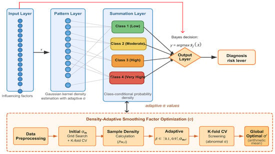
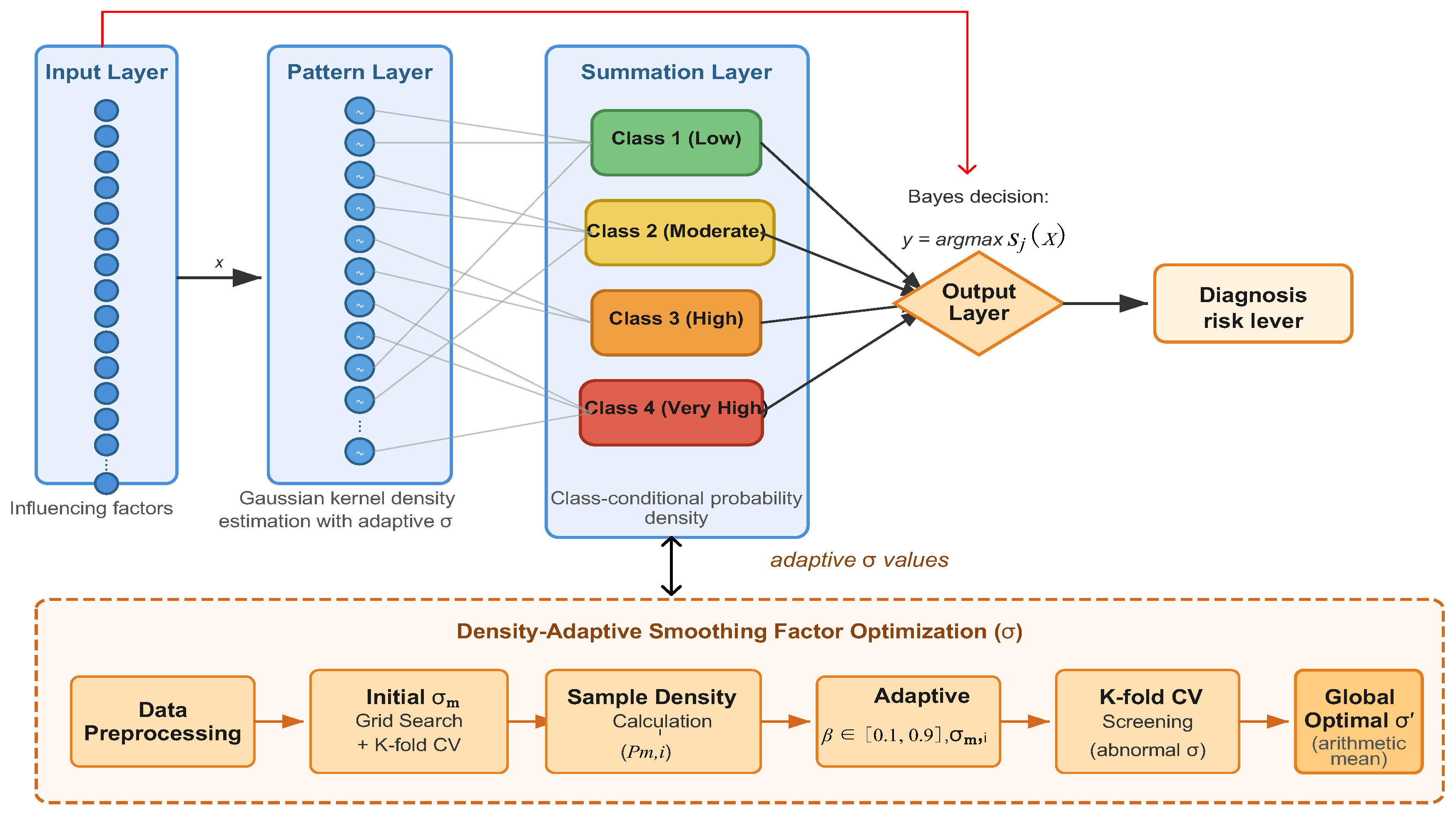
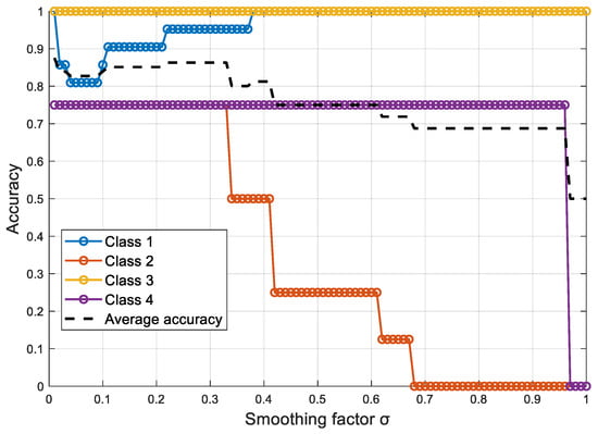
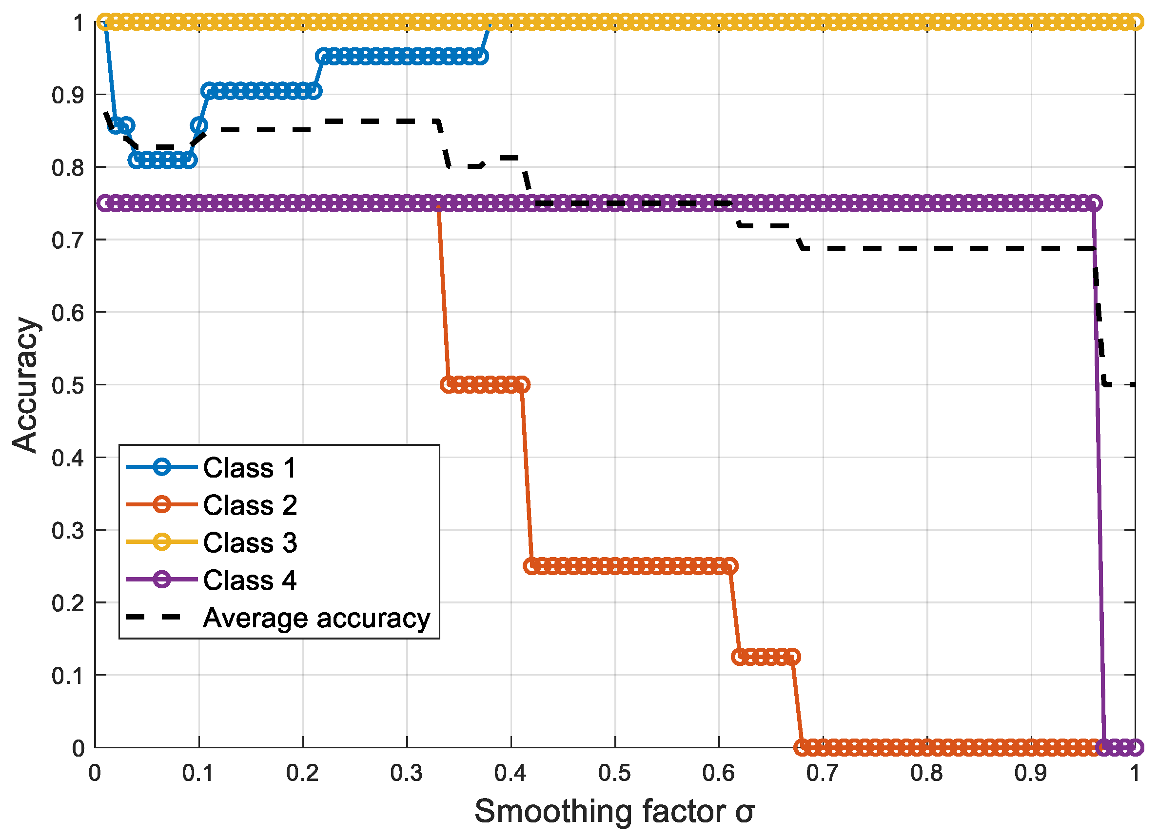
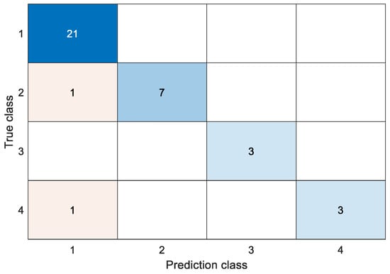
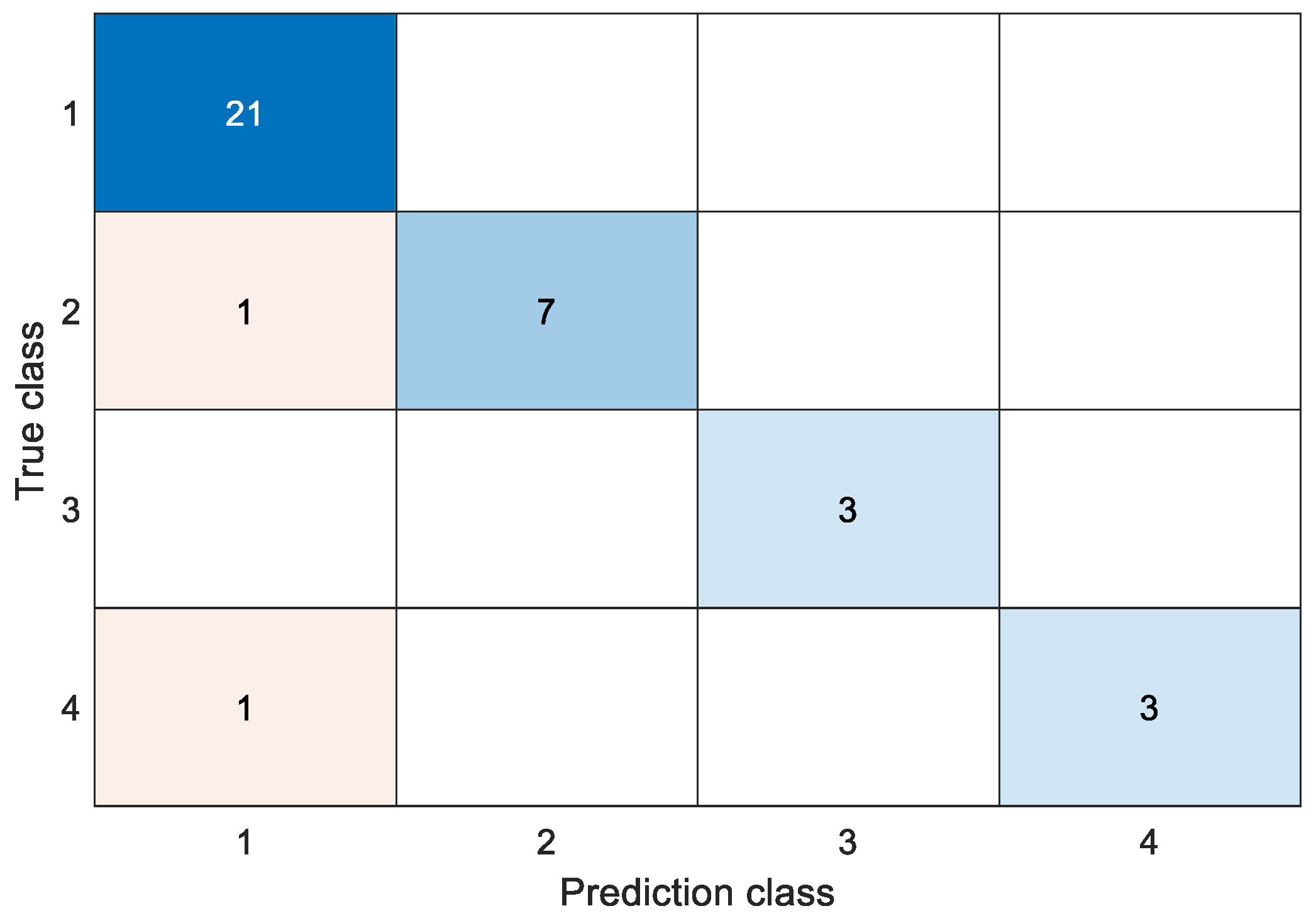
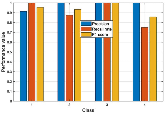
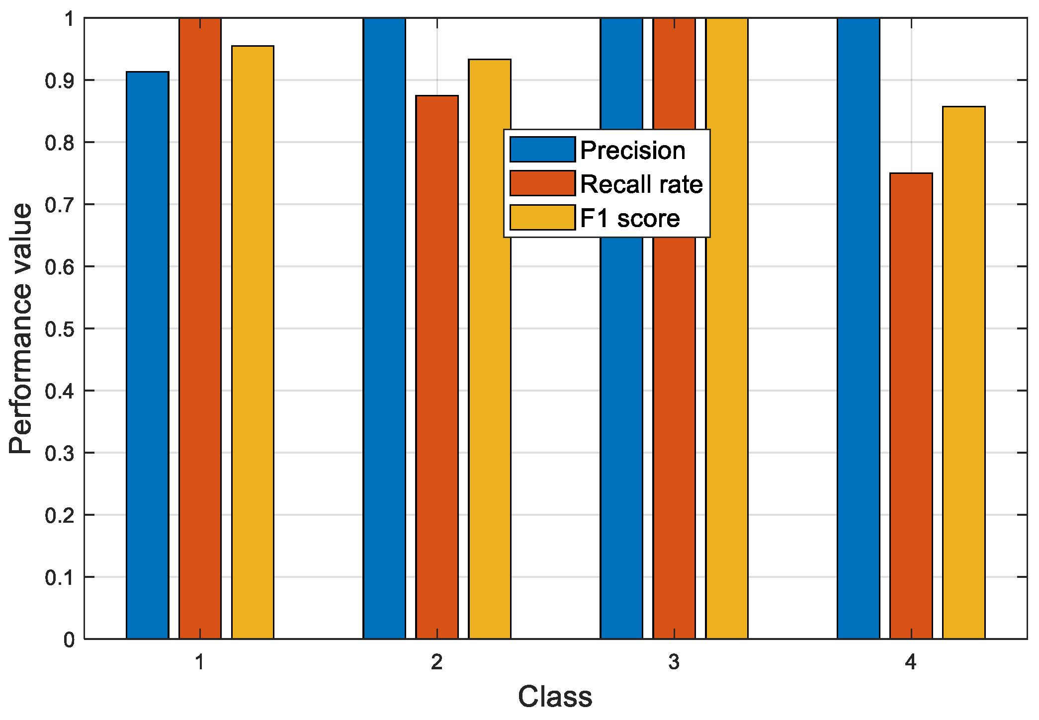
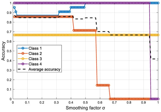
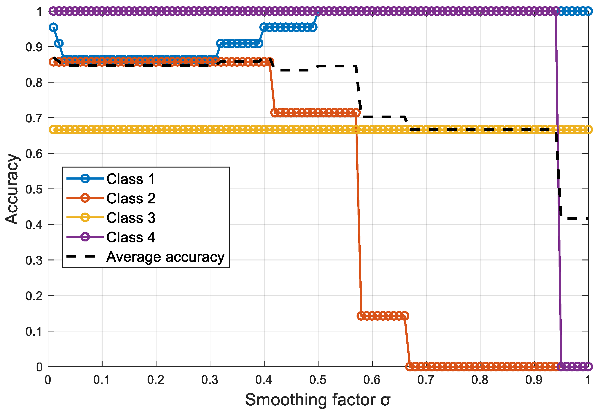
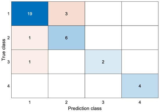
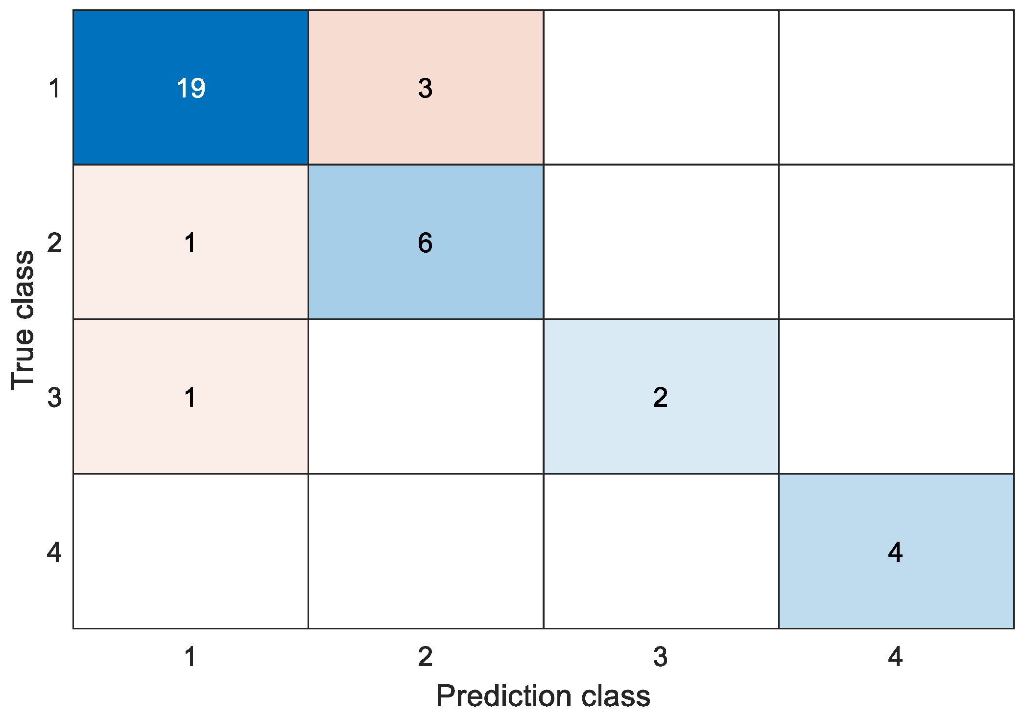
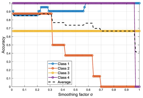
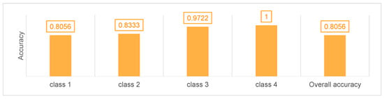
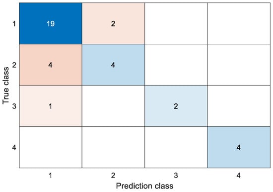
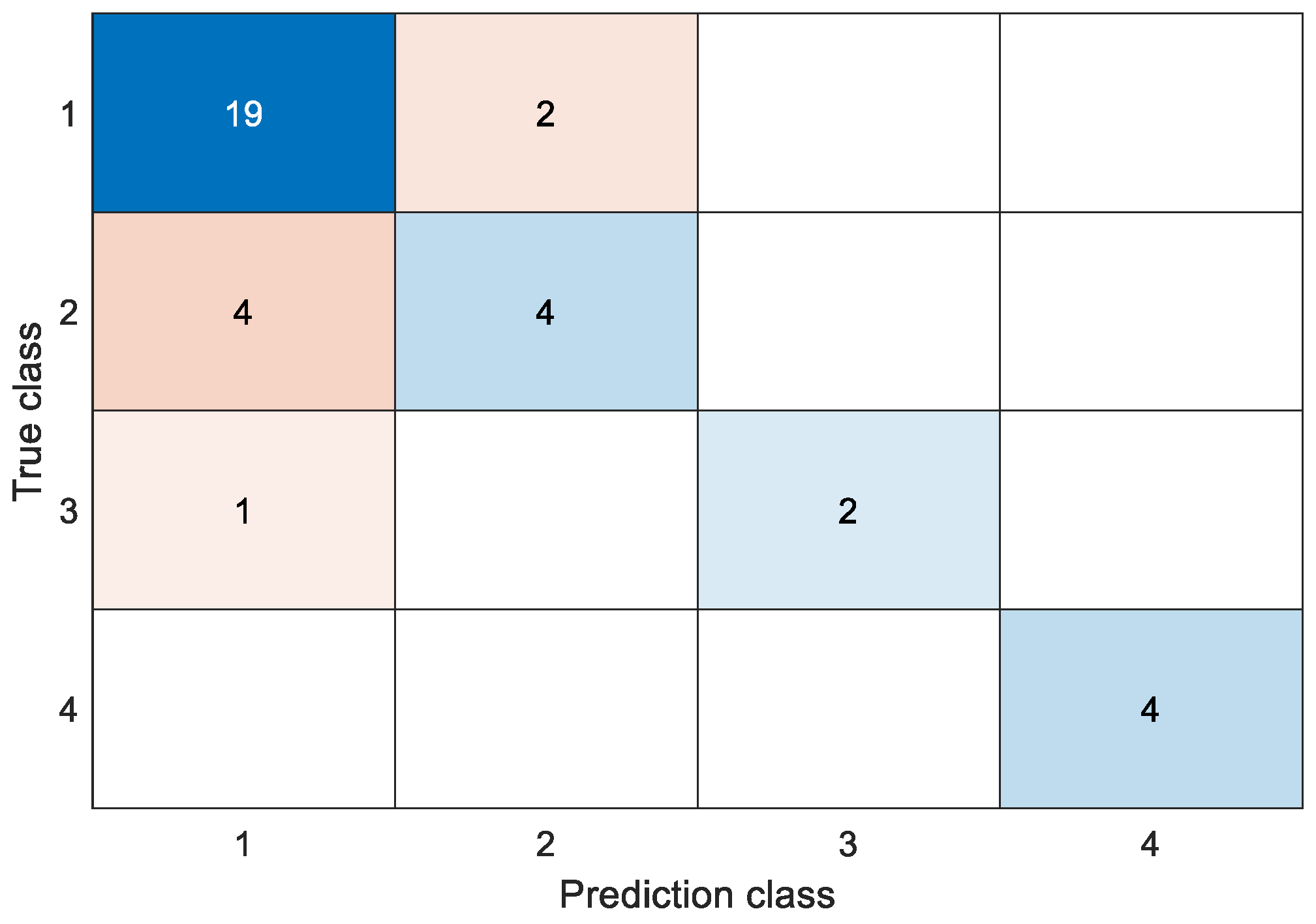
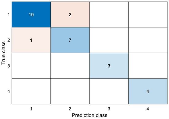
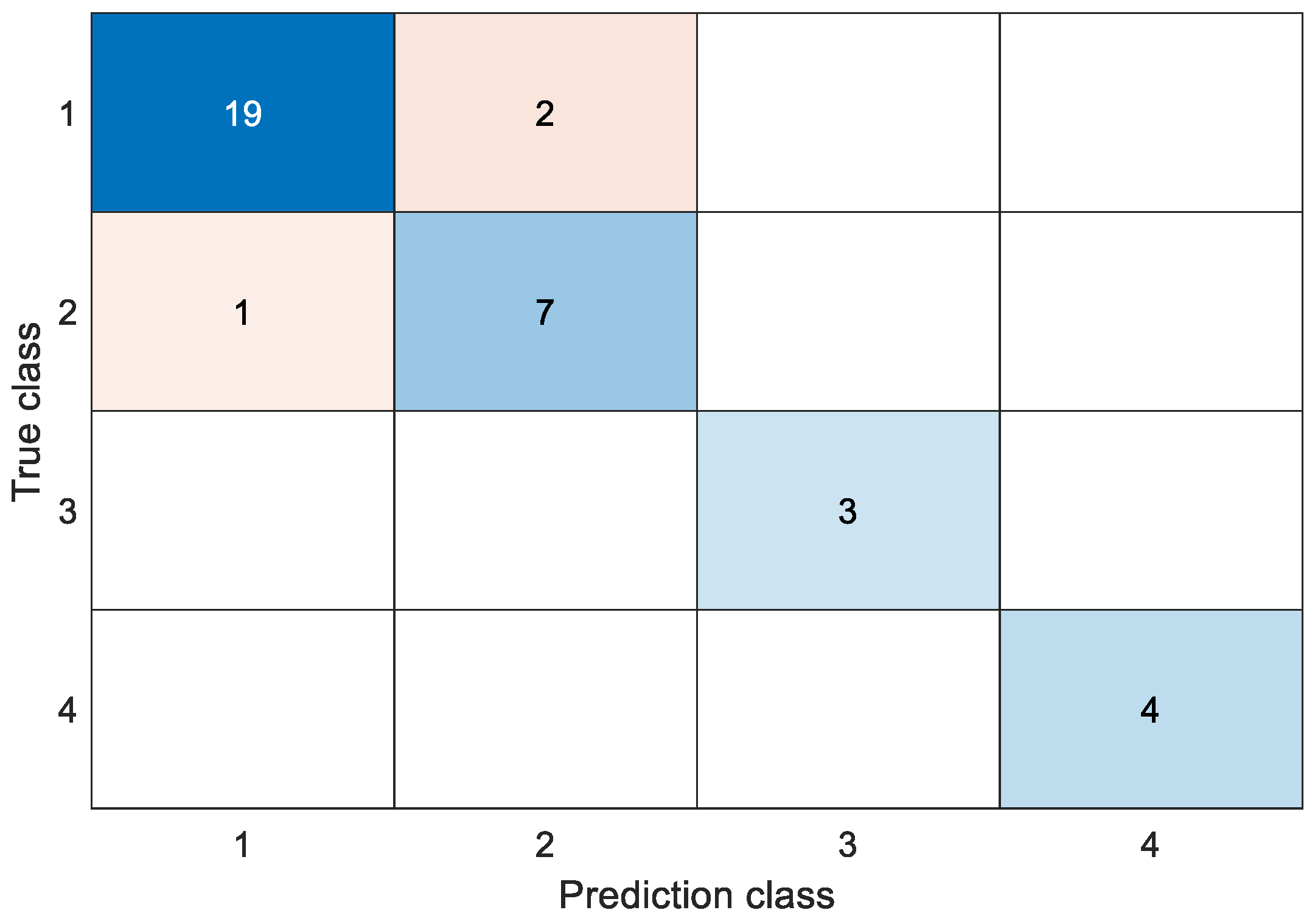
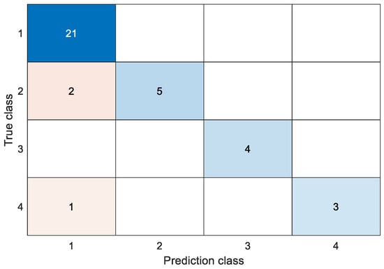
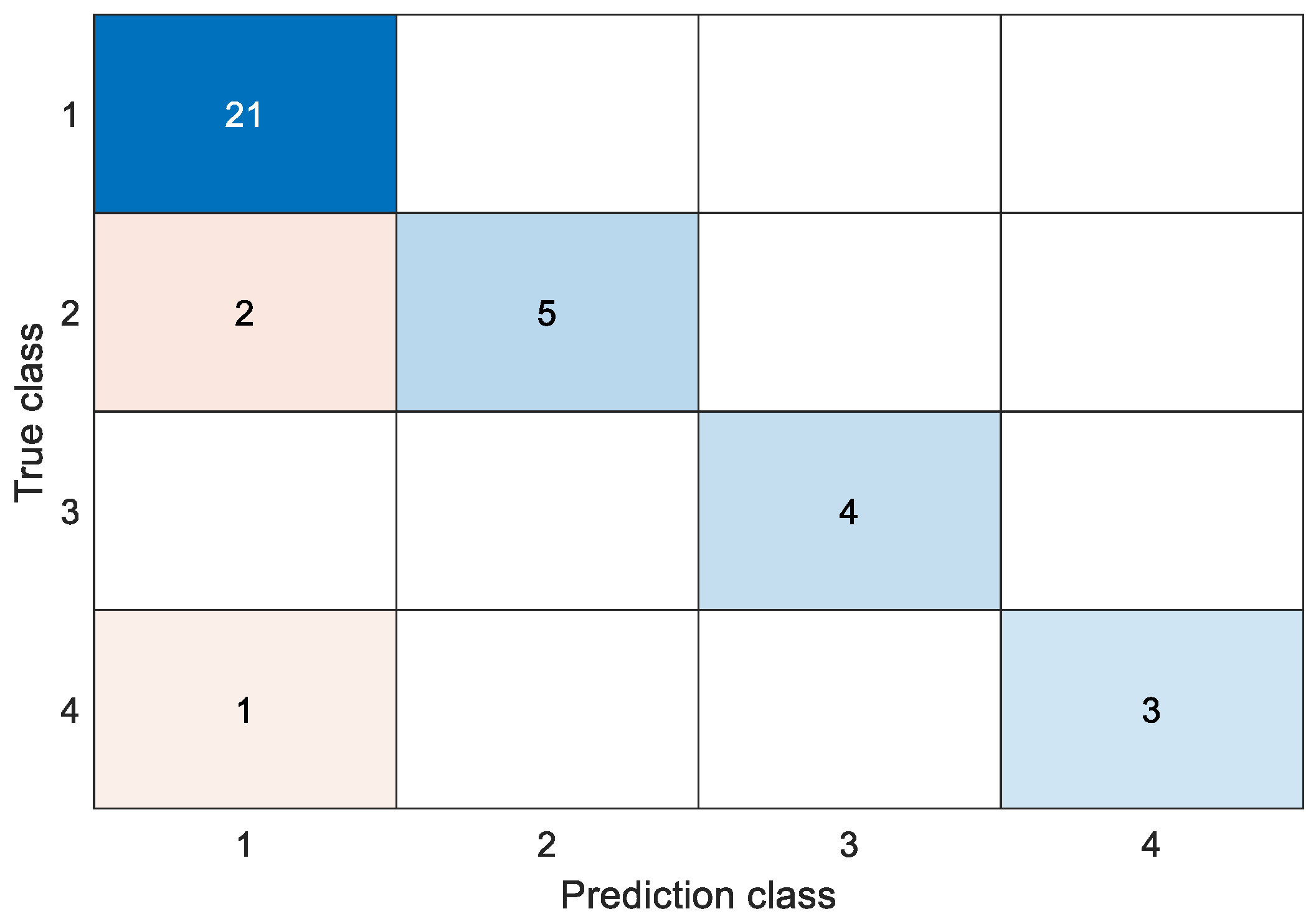
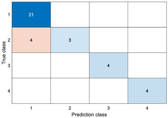
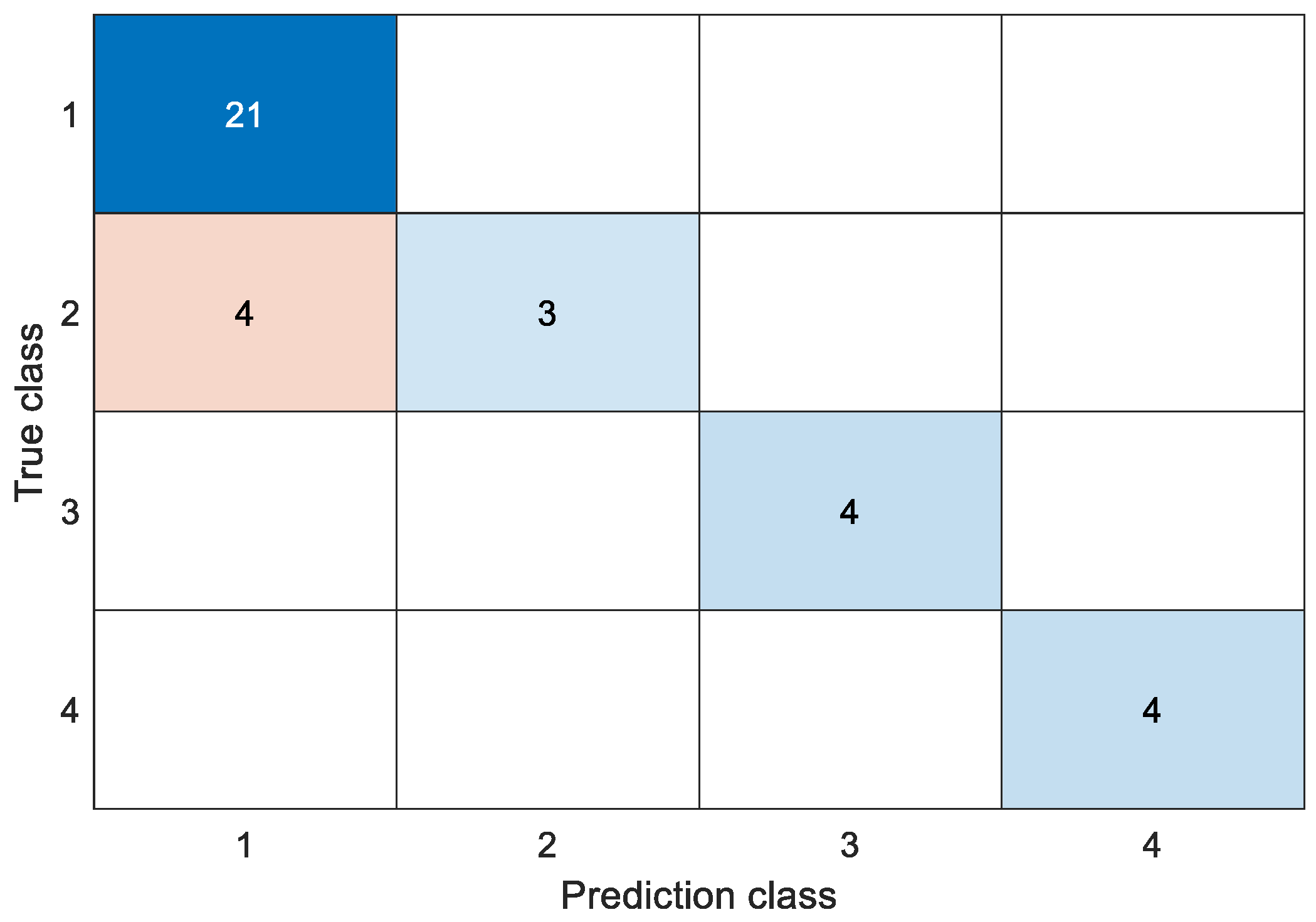
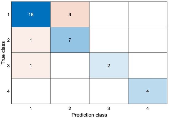
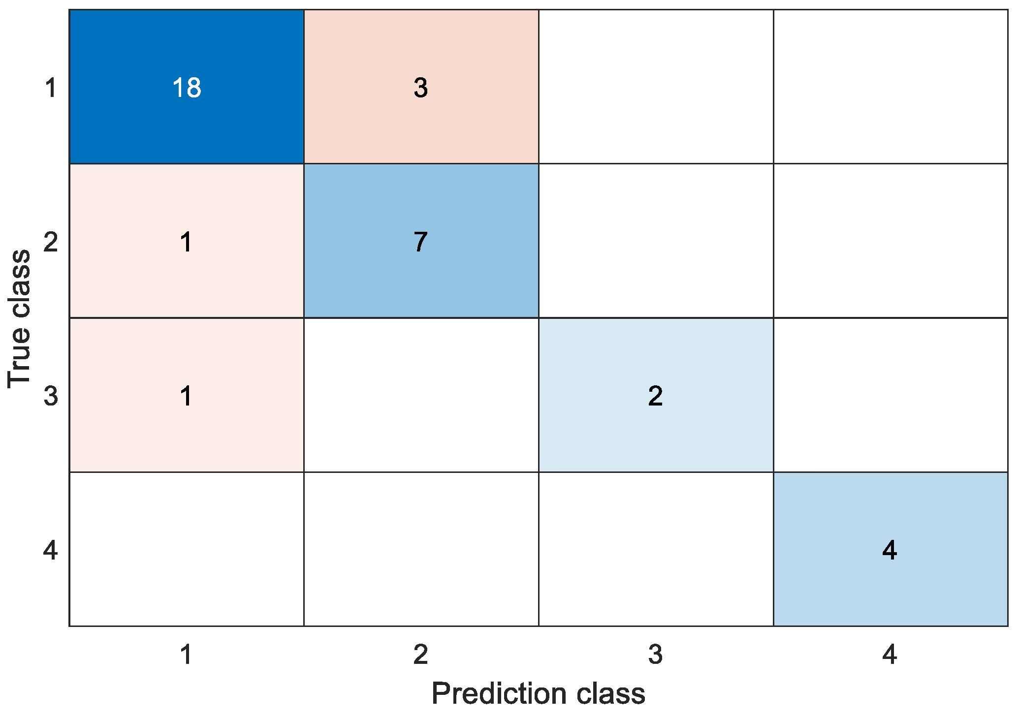
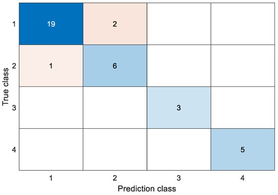
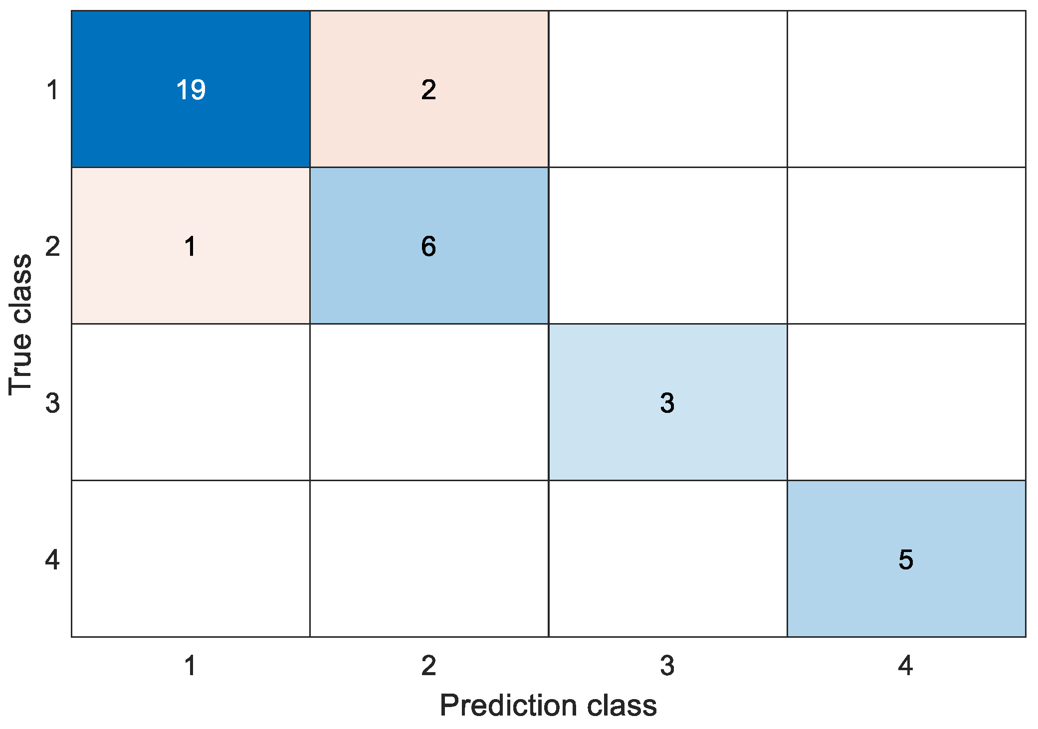
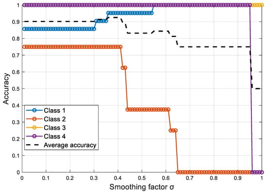
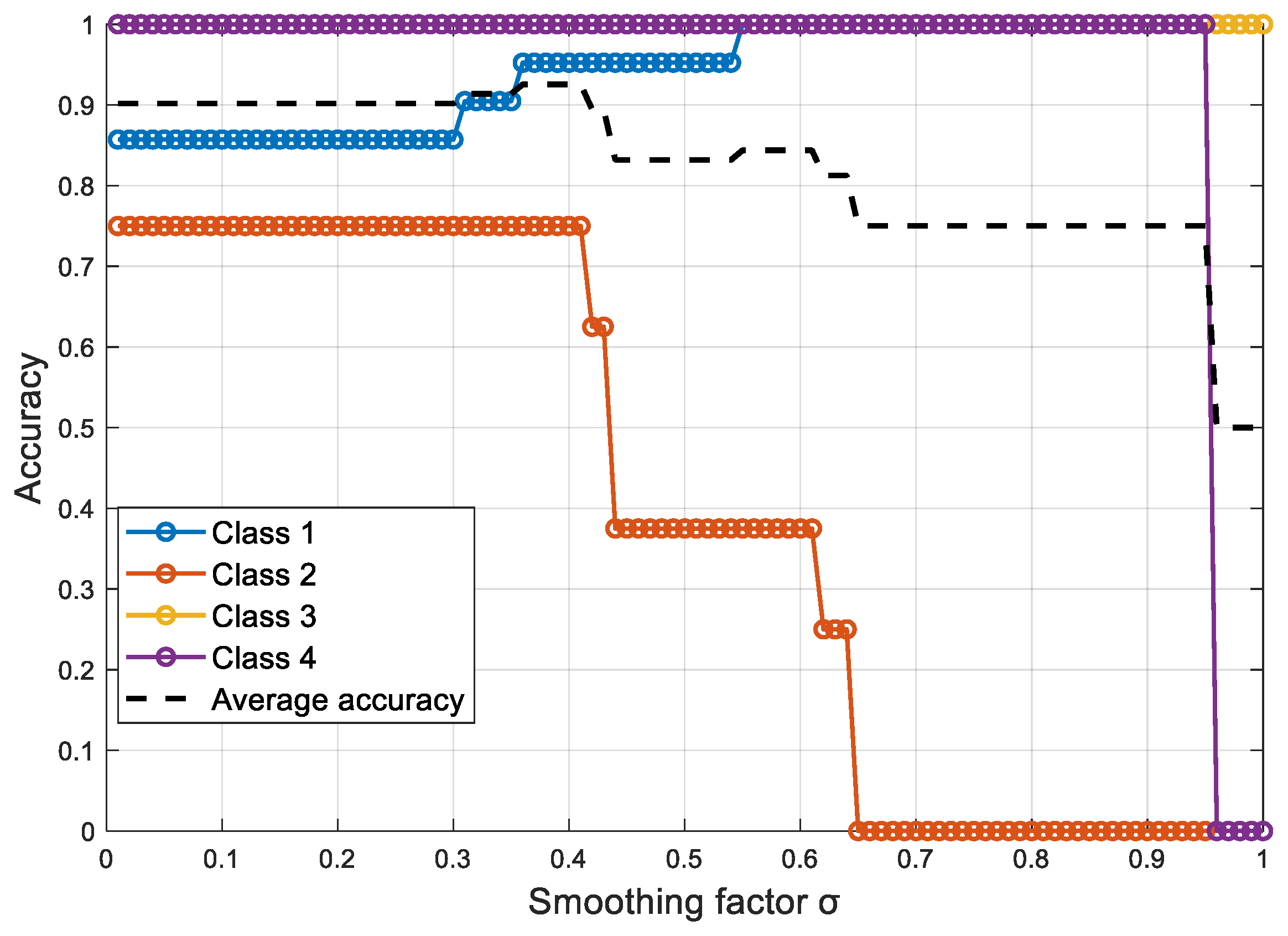
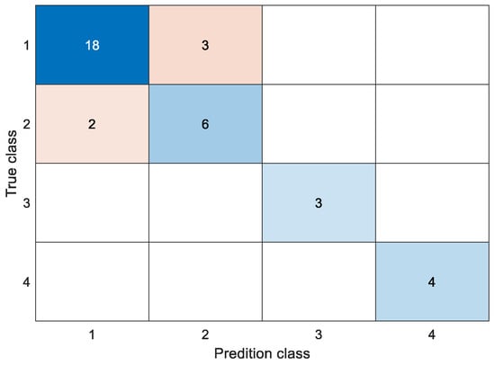
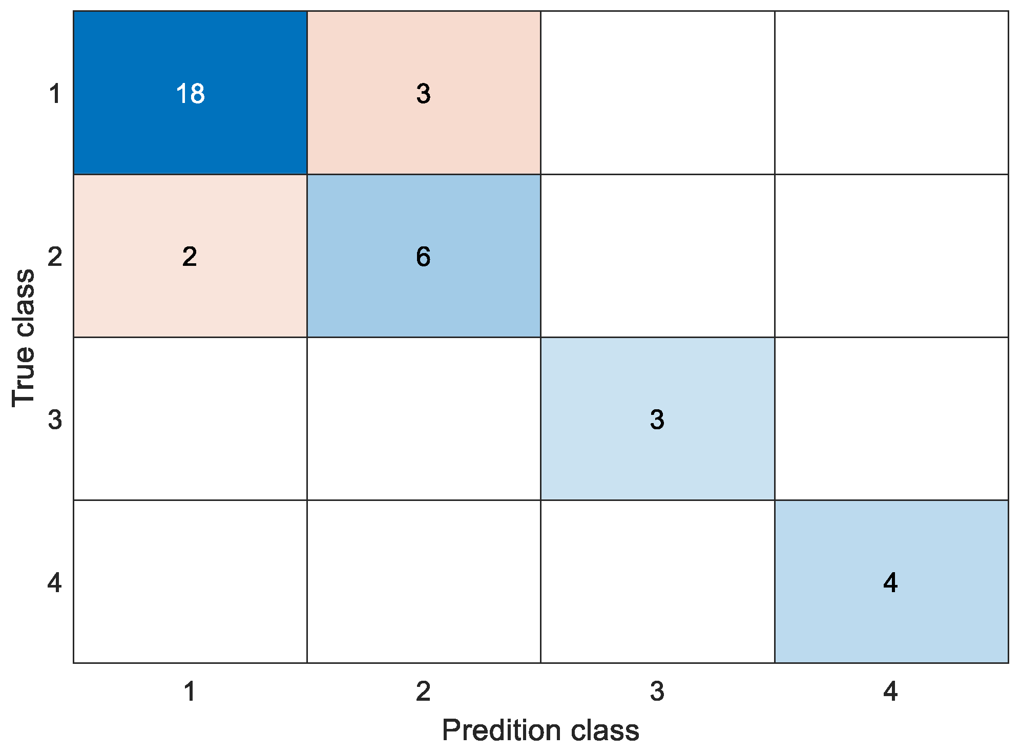
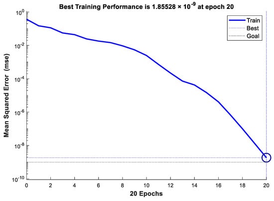
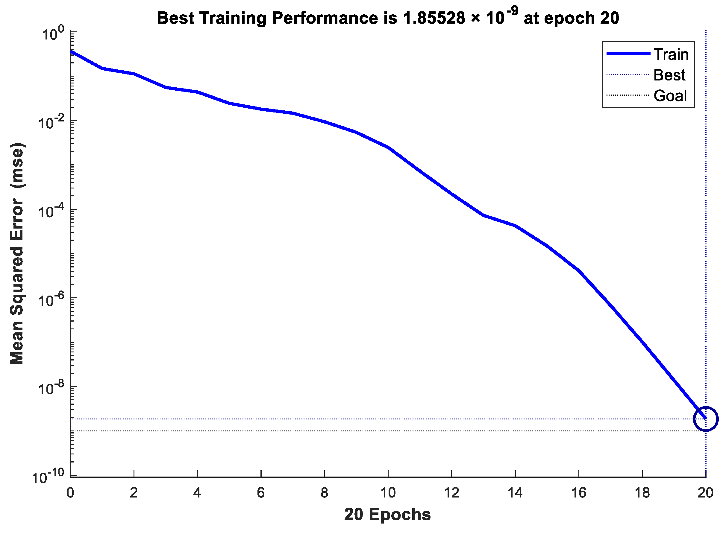
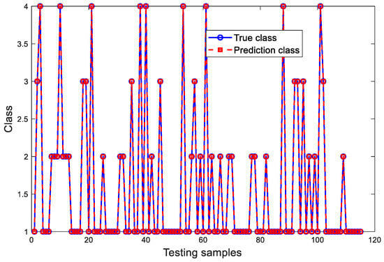
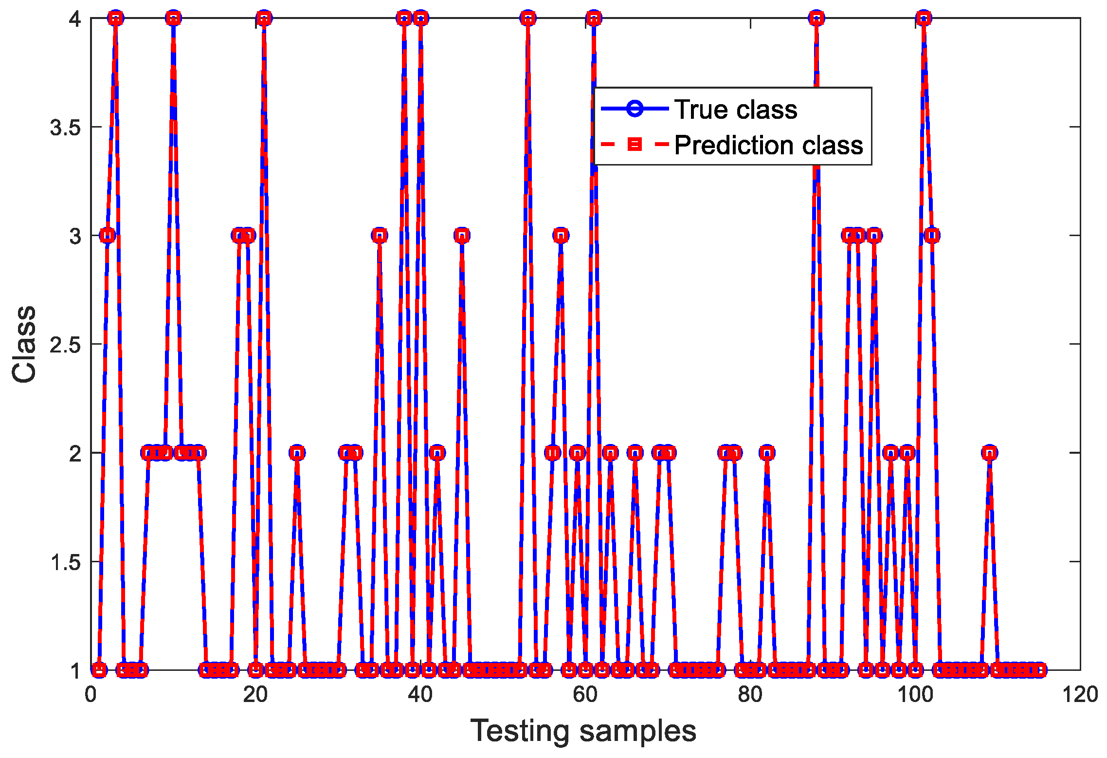
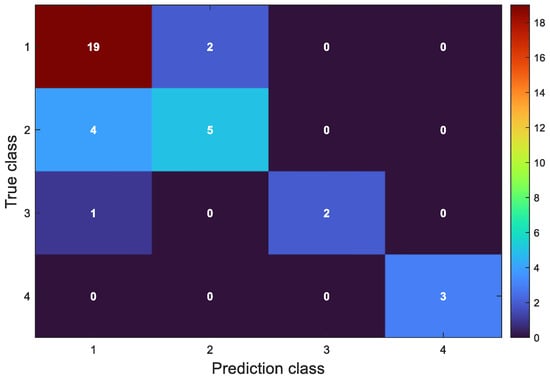
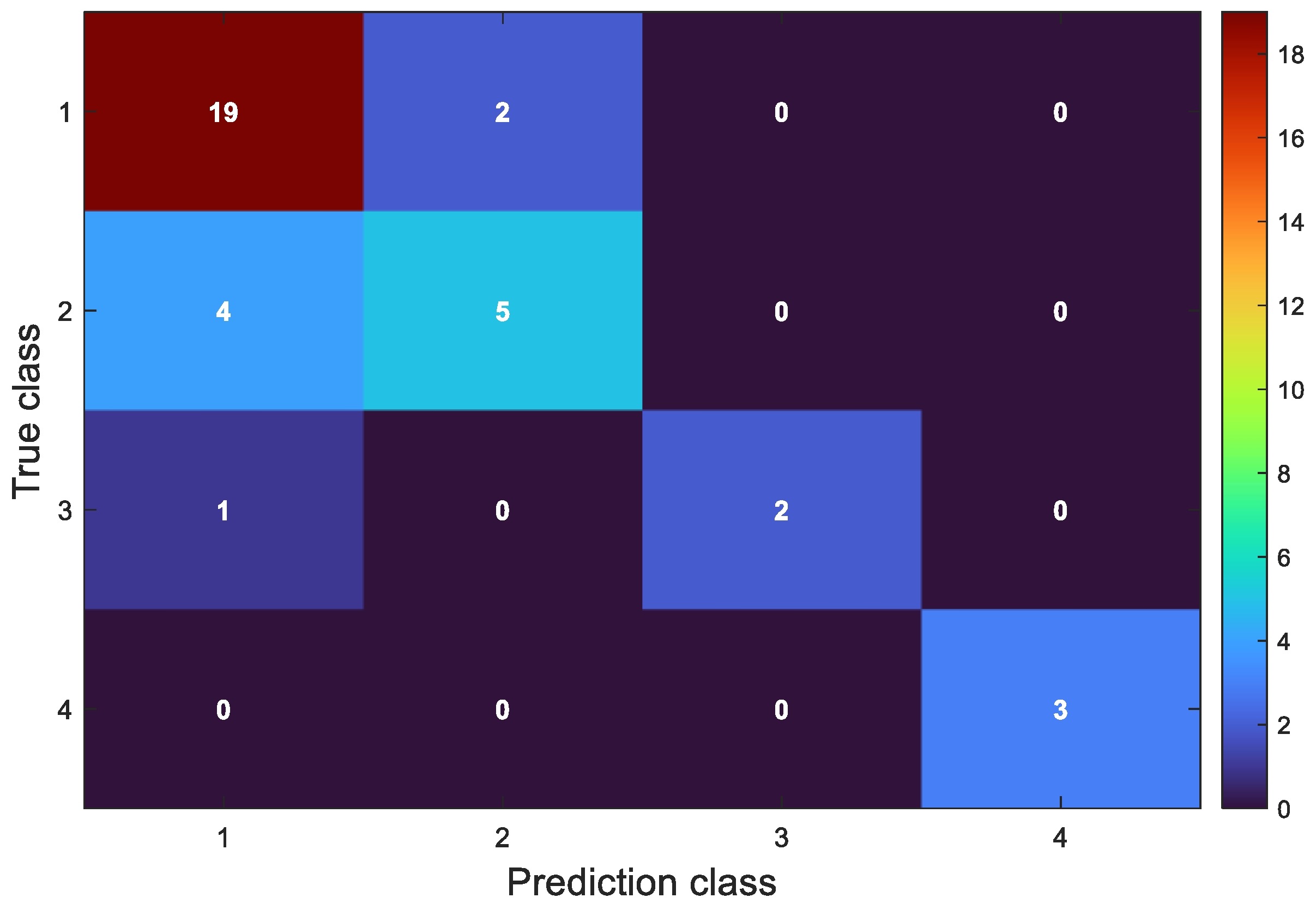
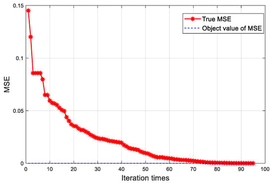
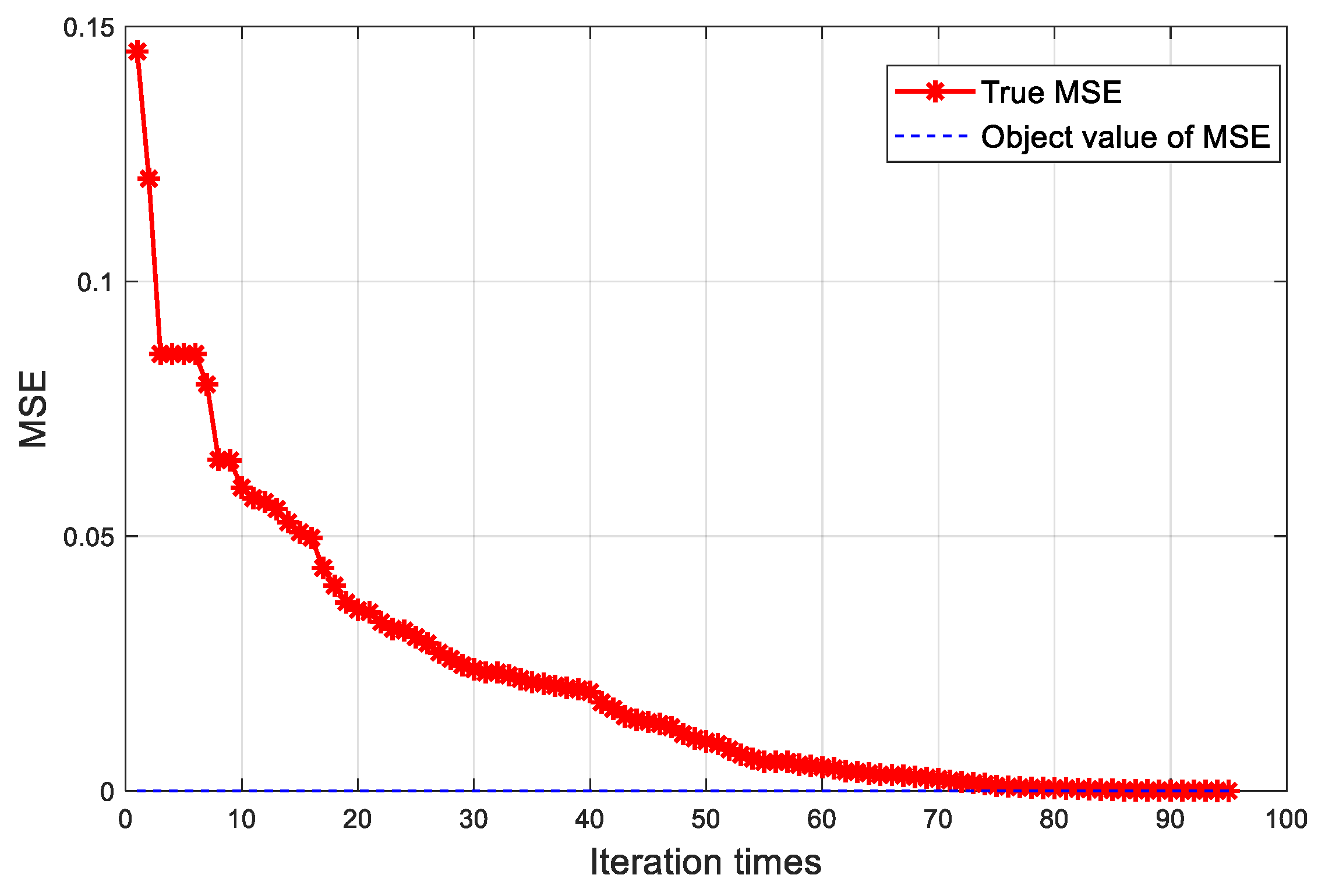
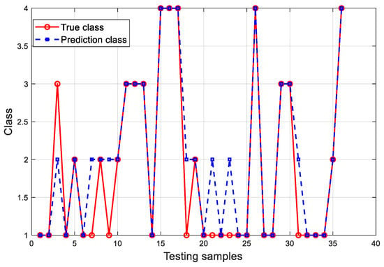
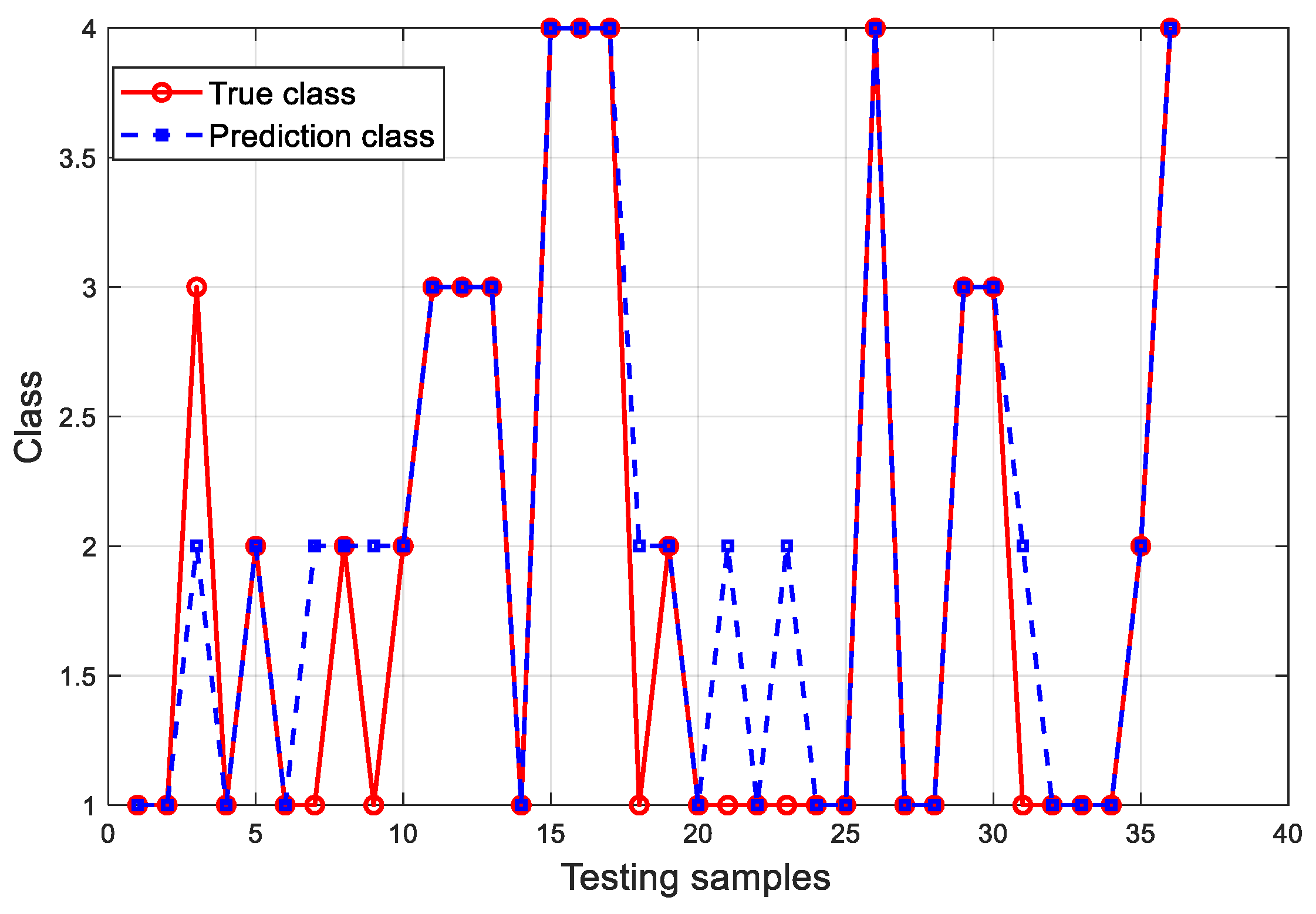
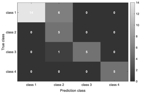
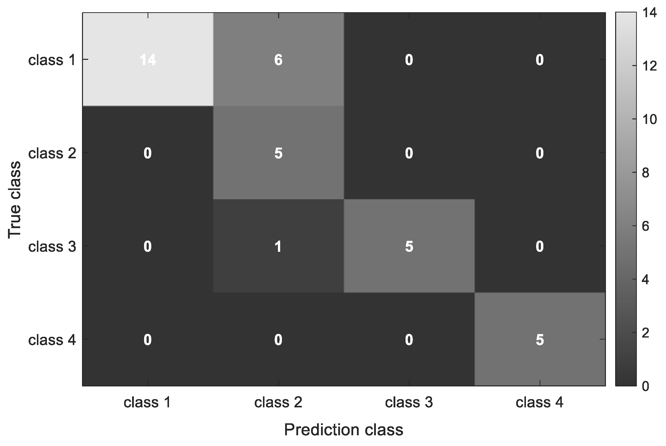

Disclaimer/Publisher’s Note: The statements, opinions and data contained in all publications are solely those of the individual author(s) and contributor(s) and not of MDPI and/or the editor(s). MDPI and/or the editor(s) disclaim responsibility for any injury to people or property resulting from any ideas, methods, instructions or products referred to in the content. |
© 2026 by the authors. Licensee MDPI, Basel, Switzerland. This article is an open access article distributed under the terms and conditions of the Creative Commons Attribution (CC BY) license.