A Joint Numerical Simulation Method for Mine Seismic–Electric Coupling

Abstract

With the continuous increase in coal mining depth in China, concealed geological structures—such as collapsed columns and faults—pose a severe threat to mine safety by triggering water inrush accidents. Mine DC resistivity methods exhibit high sensitivity to water-bearing characteristics but suffer from limited resolution, while mine seismic exploration offers superior resolution but weak sensitivity to water-rich bodies. Single-method inversion is inevitably plagued by solution non-uniqueness. This study aims to enhance the detection accuracy of concealed structures by implementing a joint seismic–electric inversion that exploits the complementary strengths of both methods. For the DC resistivity component, a forward model was established using the finite element method with unstructured meshes, and inversion was performed via Occam regularization. For seismic exploration, forward modeling employed curved-ray tracing, and inversion was conducted via the LSQR algorithm. Cross-gradient constraints were incorporated into the joint inversion to establish a structurally coupled framework. The novelty of this study lies in the integration of unstructured mesh discretization, curved-ray seismic tomography, and cross-gradient-constrained joint inversion for mine water detection. Numerical simulation results demonstrate that joint inversion effectively constrains the spatial extent of anomalies, accurately characterizes the morphology of multiple anomalous bodies and water-conducting fault channels, and substantially reduces solution non-uniqueness compared to single-method inversions. This research provides a reliable methodology for the refined detection of concealed hazard-inducing structures, offering considerable practical value for safeguarding coal mine safety.

1. Introduction

As coal mining in China progressively extends to greater depths, escalating geological complexity intensifies the risk of water inrush accidents triggered by concealed structures such as collapsed columns and faults [1,2]. These hazards pose severe threats to mine safety and personnel. Accurate characterization of the spatial distribution and water-bearing properties of such hidden structures is a prerequisite for scientific water hazard control and safe pressurized mining. Currently, borehole DC resistivity and seismic exploration have emerged as core techniques for detecting concealed underground hazards, owing to their complementary underlying physical principles.

The mine DC resistivity method, which exploits contrasts in electrical conductivity, is highly sensitive to low-resistivity anomalies such as water-bearing bodies and fractured zones, enabling effective identification of water-rich structures within roof and floor strata. However, constrained by underground-based observation configurations and limitations in inversion algorithms [3], it suffers from insufficient resolution, making it difficult to precisely delineate anomaly boundaries; this often leads to boundary smearing and false anomalies, particularly in environments with multiple overlapping targets. Mine seismic exploration, which relies on seismic impedance contrasts, offers high resolution and a superior signal-to-noise ratio, excelling at characterizing structural interfaces and rock mass integrity. Nevertheless, it is relatively insensitive to variations in water content, rendering it ineffective for distinguishing between dry and water-saturated structures. The inherent limitations of individual geophysical methods result in significant interpretation ambiguity, failing to meet the demands for high-precision exploration in modern intelligent mining [4]. Joint inversion, which integrates multiple geophysical methods to achieve data complementarity and mutual constraints, has emerged as a key technology for overcoming the limitations of individual techniques. Since Vozoff and Jupp pioneered true joint inversion, related research has evolved from one-dimensional layered models to three-dimensional complex structures and from linear to nonlinear approaches [5]. Lines et al. employed the least-squares method for joint inversion and compared the merits of sequential and synchronous strategies [6]. In 1995, Hering et al. proposed the first 1D joint inversion formulation for DC resistivity and seismic surface-wave data, laying the theoretical groundwork for subsequent seismic–electric inversion [7]. Kis et al. further realized the joint inversion of multiple wave types and DC apparent resistivity for 2D geological bodies [8]. Gallardo and Meju have conducted extensive systematic research in this field; their proposed cross-gradient constraint theory avoids presupposing empirical relationships between petrophysical parameters. Instead, it enhances the structural consistency of different property models to achieve joint inversion, significantly improving accuracy and reliability [9]. This method has since been widely applied in studies such as 3D joint inversion of potential field data.

In China, Yu Peng and colleagues summarized the application conditions for joint inversion through extensive research [10]. Chen Xiao and Yu Peng introduced regularization and adaptive techniques into synchronous joint inversion, enhancing solution stability and computational efficiency [11]. Zhou Lifen employed cross-gradient theory to couple resistivity and seismic velocity data, achieving 2D synchronous joint inversion of magnetotelluric and seismic data [12]. Gao Ji and Zhang Haijiang developed a joint inversion scheme for seismic traveltime and DC resistivity data with cross-gradient constraints, effectively mitigating shadow zone issues in seismic body-wave tomography and DC resistivity imaging [13]. Peng Miao and Tan Handong et al. conducted three-dimensional joint inversion of magnetotelluric and seismic traveltime data with cross-gradient constraints. The study demonstrated that joint inversion enhanced the recovery degree of deep velocity structure characteristics of abnormal bodies [14]. These domestic studies have confirmed the feasibility of applying cross-gradient theory to seismic–electric joint inversion.

However, it is crucial to acknowledge the inherent limitations of these advances, particularly concerning the reliance on synthetic models and idealized theoretical assumptions. Firstly, most existing validations are predicated on simplified synthetic models that assume homogeneous backgrounds and regular anomaly geometries. While instructive, such models often fail to capture the extreme heterogeneity, anisotropic characteristics, and irregular interfaces prevalent in real mining environments. Consequently, the performance of joint inversion algorithms may degrade when confronted with actual geological complexities. Secondly, the theoretical framework of cross-gradient constraints assumes a strict structural coupling between different physical properties. In practice, however, this correlation may be weak or non-existent in certain geological settings (e.g., where fracturing occurs without significant fluid infiltration), potentially leading to biased inversion results if enforced indiscriminately. Finally, the computational overhead associated with high-fidelity forward modeling and inversion in complex 3D mine spaces remains a significant bottleneck, limiting the current transition from theoretical models to real-time field applications.

A critical assessment shows that existing studies primarily focus on general geophysical scenarios. Significant gaps remain regarding adaptation to the confined spaces and complex boundaries (e.g., roadway interference) of underground mines, and there is a lack of targeted research on typical hazardous structures like water-conducting collapsed columns and faults. Moreover, the critical balance between inversion accuracy and computational efficiency under deep mining conditions remains unresolved. Concurrently, the advancement of intelligent mining has intensified electromagnetic interference, challenging the robustness of current methods against practical operational conditions.

The inherent complementarity between mine DC resistivity and seismic exploration provides a natural foundation for accurately detecting concealed hazardous structures. Consequently, this paper focuses on developing a 2D mine-adapted seismic–electric joint inversion method. We aim to optimize structural coupling constraints and inversion algorithms. Through numerical simulations based on theoretical models of various anomalies and typical disaster-inducing structures, we seek to establish a joint inversion framework suited to complex mine conditions. Recognizing the aforementioned limitations, we emphasize that while our numerical experiments utilize synthetic data to validate the methodology, the ultimate goal is to bridge the gap between idealized models and field applications. This work is intended to provide a reliable technical pathway for the precise detection of concealed geological hazards, thereby offering robust support for intelligent mine construction and safety in production. The novel contribution of this study lies in the integration of unstructured mesh discretization, curved-ray seismic tomography, and cross-gradient-constrained joint inversion within a unified framework specifically tailored for underground mine environments, which distinguishes this work from previous joint inversion studies focused on general geophysical applications.

2. Individual Inversion

2.1. Mine DC Resistivity Method

2.1.1. Resistivity Method Forward Modeling

Based on the variational formulation of the steady-state current equation, the boundary value problem governing electrical potential distribution is discretized. This meshing strategy allows for localized refinement in areas with high potential gradients, ensuring both computational accuracy and efficiency.

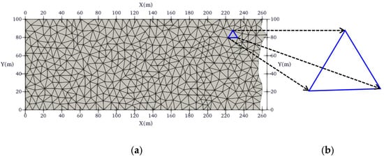
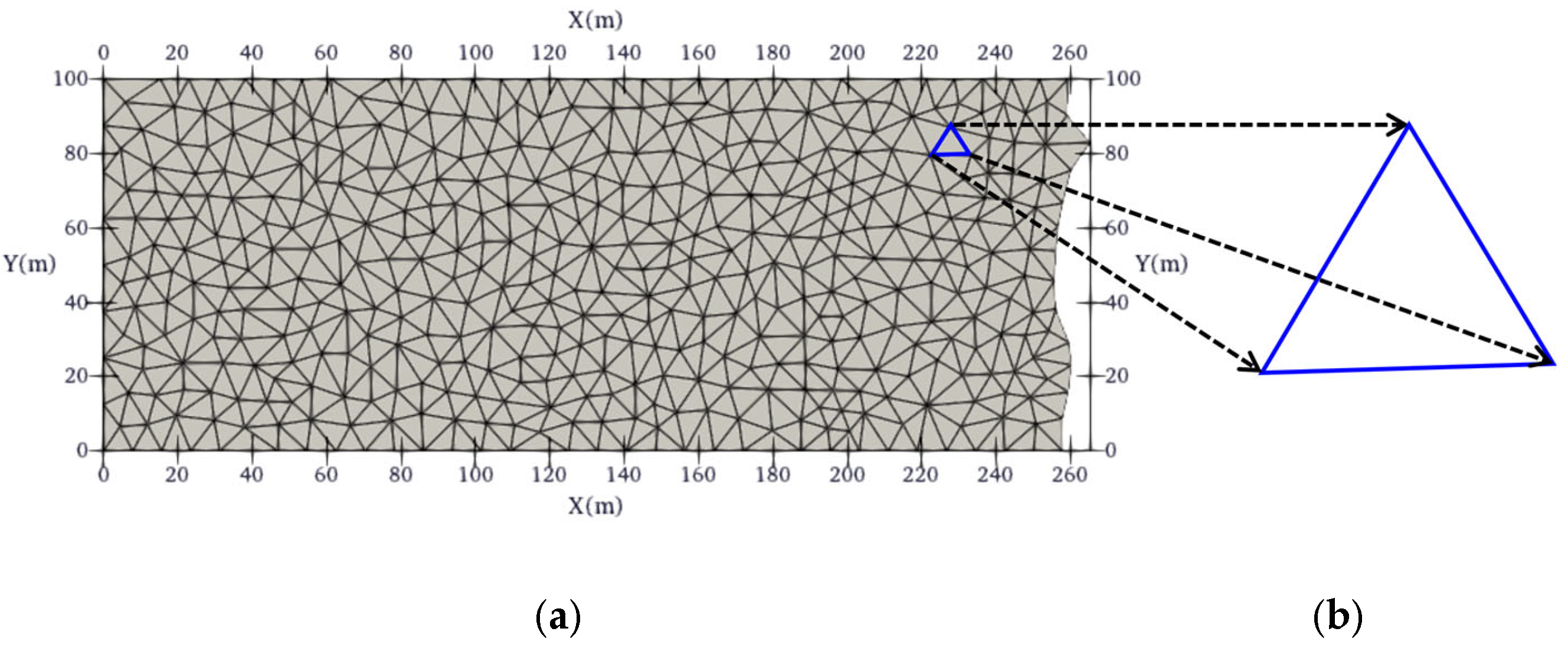
The forward model is constructed using the finite element method (FEM) with an unstructured triangular mesh. The computational domain is discretized into triangular elements to accurately conform to complex geological geometries and roadway boundaries encountered in underground mining environments, as shown in Figure 1 [15].

Figure 1. Unstructured triangular mesh. (a) Part of a coal seam unstructured triangular mesh and (b) cell of a triangular mesh.

Based on the variational formulation of the steady-state current equation, the boundary value problem governing the electrical potential distribution is discretized using the finite element method [16]. Discretization yields a large, sparse linear algebraic system:

$$\nabla \cdot \left(\sigma \nabla \mathit{U}\right)=-2\mathit{I}\delta \left(A\right)\hspace{1em}\in \mathsf{\Omega },$$

(1)

$${\displaystyle \frac{\partial \mathit{U}}{\partial n}}=0\hspace{1em}\hspace{1em}\hspace{1em}\hspace{1em}\hspace{1em}\hspace{1em}\hspace{1em}\hspace{1em}\hspace{1em}\in {\mathsf{\Gamma }}_s,$$

(2)

$${\displaystyle \frac{\partial \mathit{U}}{\partial n}}+{\displaystyle \frac{\cos \left(r,n\right)}{r}}\mathit{U}=0\hspace{1em}\hspace{1em}\hspace{1em}\hspace{1em}\hspace{1em}\hspace{1em}\hspace{1em}\hspace{1em}\in {\mathsf{\Gamma }}_{\mathrm{\infty }}$$

(3)

where σ denotes the electrical conductivity of the subsurface medium, δ represents the Dirac delta function, n is the coordinate variable in the outward normal direction of the boundary, r is the position vector from the source point to a boundary point, Ω signifies the computational domain, and Γ_s and Γ_∞ refer to the ground surface and subsurface boundaries, respectively.

Linear basis functions are adopted for interpolation within each triangular element. Integral results of all elements are assembled to derive the global matrix system:

$$\begin{array}{cc}\mathrm{F}\left(\mathbf{U}\right)& =\sum {\mathrm{F}}_e(\mathbf{U})=\sum {\displaystyle \frac{\sigma }{2}}{U}_e^{\mathrm{T}}\left(K_{1e}+K_{2e}\right){\mathit{U}}_e-{\mathit{U}}_A\mathit{I}\\ & ={\displaystyle \frac{1}{2}}{U}_e^{\mathrm{T}}K\mathit{U}-{\mathit{U}}^{\mathrm{T}}\mathit{P}\hfill \end{array}$$

(4)

where U denotes the global nodal potential vector. According to the variational extremum principle, setting the first variation of Equation (4) to zero generates the linear algebraic system:

$$\mathit{K}\mathit{U}=\mathit{P}$$

(5)

The symmetric successive over-relaxation (SSOR) scheme is employed to construct a preconditioner for the conjugate gradient (CG) method [17], enabling efficient iterative solution of the large, sparse linear system. Drawing upon the incomplete Cholesky decomposition-preconditioned biconjugate gradient strategy as a reference, the SSOR preconditioner is optimized using sparse matrix storage techniques [18]. The nodal potential distribution U across the target domain is then solved via CG iteration. This scheme maintains computational accuracy while substantially improving solver efficiency for large-scale problems. However, it should be noted that the convergence rate of CG methods depends on the condition number of the stiffness matrix, which can be adversely affected by mesh quality and model complexity. In mine environments with highly irregular geometries, additional mesh refinement near source locations may be required to ensure numerical stability [19].

2.1.2. Resistivity Method Inversion Algorithm

The inversion problem is formulated as a regularized least-squares optimization problem. The objective function is established based on the Occam inversion algorithm [20] to balance data-fitting accuracy and model smoothness. This approach seeks the smoothest model that adequately fits the observed data, effectively mitigating the inherent ill-posedness of the DC resistivity inverse problem. The regularization parameter λ is dynamically adjusted using the L-curve criterion or the generalized cross-validation method to achieve an optimal balance between data misfit and model smoothness [21].

$$\mathsf{\Phi }=(\Delta \overrightarrow{d}-J\overrightarrow{m}{)}^T(\Delta \overrightarrow{d}-J\overrightarrow{m})+\lambda (R\overrightarrow{m}{)}^T(R\overrightarrow{m})$$

(6)

where Δd is the residual vector between field observations and theoretical forward data, m denotes the model parameter vector, J represents the sensitivity (Jacobian) matrix, λ is the dynamically adjusted regularization parameter, and R signifies the model roughness matrix.

The model parameter update equation is expressed as

$$\Delta \overrightarrow{m}=(J^{T}J+\lambda R^{T}R{)}^{-1}J\Delta \overrightarrow{d}$$

(7)

In DC resistivity inversion, the root mean square (RMS) error is a critical indicator for evaluating the consistency between model responses and field measurements. It quantifies the overall deviation between theoretical calculations and observed data, providing an objective criterion for inversion reliability. The inversion convergence is defined as the relative change rate of the RMS error being less than 2%, and the RMS error is formulated as

$$RMS=\sqrt{{\displaystyle \frac{1}{N}}{\sum }_{i=1}^N({\displaystyle \frac{d_i-f(\overrightarrow{m}{)}_i}{d_i}}{)}^2}\times 100$$

(8)

where N is the number of observation data points, $d_i$ is the $i$-th measured datum, and $f(\overrightarrow{m}{)}_i$ represents the theoretical response corresponding to the model parameters.

2.2. Mine Seismic Exploration

2.2.1. Seismic Method Forward Modeling

Unstructured mesh discretization is performed via Delaunay triangulation [22,23], which ensures optimal mesh quality by maximizing the minimum angle of all triangles and avoiding overly slender elements. The squared slowness (the reciprocal of velocity squared, 1/v²) is adopted as the model parameter to accurately capture complex geological interfaces in underground mining environments [24,25]. Based on Fermat’s principle of minimum traveltime, a curved-ray tracing method is utilized to simulate seismic wave propagation paths, iteratively correcting ray trajectories to align with true paths via the variational principle [26,27]. This curved-ray approach provides more accurate traveltime calculations compared to straight-ray methods, particularly in heterogeneous media with strong velocity variations commonly encountered in mine environments. with squared slowness (the reciprocal of velocity squared, 1/v²) adopted as the model parameter to accurately capture complex geological interfaces in underground mining environments [24,25]. Based on Fermat’s principle of minimum traveltime, a curved-ray tracing method is utilized to simulate seismic wave propagation paths, iteratively correcting ray trajectories to align with true paths via the variational principle [26].

The governing forward equation system is expressed as

$${\sum }_{j=1}^M{L}_{ij}{s}_j=t_i(i=\mathrm{1,2},\dots ,N)$$

(9)

In Equation (9), $L_{ij}$ denotes the length of the $i$-th ray traversing the $j$-th grid cell, $s_j$ represents the squared slowness of the $j$-th cell, $t_i$ is the traveltime of the $i$-th ray $M$, is the total number of grid cells, and $N$ is the total number of rays. Solving this system yields theoretical traveltime datasets.

2.2.2. Seismic Method Inversion Algorithm

The LSQR algorithm (least-squares QR decomposition) is employed to solve large, sparse linear systems [28,29]. By exploiting matrix sparsity, the computational load is drastically reduced, memory consumption is minimized, and numerical instability inherent in conventional least-squares methods is avoided; the algorithm exhibits linear convergence characteristics. This method is based on the Lanczos bidiagonalization process, iteratively constructing orthogonal matrices to transform the original system into bidiagonal form, which is then solved via QR decomposition [29]. The reliability of LSQR for seismic tomography has been extensively validated in numerous applications, providing stable solutions even for ill-conditioned systems that arise from uneven ray coverage [20]. It is widely employed to solve large, sparse linear systems. By exploiting matrix sparsity, the computational load is drastically reduced, memory consumption is minimized, and numerical instability inherent in conventional least-squares methods is avoided; the algorithm exhibits linear convergence characteristics. This method is based on the Lanczos bidiagonalization process, iteratively constructing orthogonal matrices to transform the original system into bidiagonal form, which is then solved via QR decomposition [28].

The inversion objective function is formulated as

$$\mathrm{m}\mathrm{i}\mathrm{n}\Vert Ax={b\Vert }_2$$

(10)

where $\mathbf{A}$ is the coefficient matrix containing ray segment lengths, x denotes the squared slowness parameter vector, and b is the traveltime residual vector. The algorithm iteratively constructs orthogonal matrices and updates model parameters until the residuals decline to the observational error level and satisfy predefined accuracy criteria.

3. Joint Inversion

3.1. Joint Inversion Model

A synchronous joint multi-parameter inversion (SJIMM) framework is employed, formulating an objective function that integrates a data misfit term, a model regularization term, and a structural constraint term to achieve collaborative inversion of DC resistivity and seismic data [30]:

$${\phi }_{SJIMM}\left(\mathbf{m}\right)={\displaystyle {\sum }_{i=1}^A} {\phi }_{\left(d,i\right)}\left({\mathbf{m}}_{\left(j\right)}\right)+{\displaystyle {\sum }_{j=1}^B} {\mu }_{\left(j\right)}{\phi }_{\left(m,j\right)}\left({\mathbf{m}}_{\left(j\right)}\right)+{\displaystyle {\sum }_{l=1}^C} {\beta }_{\left(l\right)}{\psi }_{\left(l\right)}\left(\mathbf{m}\right)$$

(11)

where the parameters are defined as follows:

${\phi }_{\left(d,i\right)}\left(\mathit{m}\right)$: residual norm;

A: total number of independent observation datasets;

B: number of inverted petrophysical parameters;

C: number of coupling constraints between parameters;

$\mathbf{m}={\left[{\mathbf{m}}_{\left(1\right)},{\mathbf{m}}_{\left(j\right)},\cdots ,{\mathbf{m}}_{\left(B\right)}\right]}^T$: model parameter vector;

${\mu }_{\left(j\right)}$: regularization parameter;

${\beta }_{\left(l\right)}$: weight coefficient of the $l$-th model constraint function;

${\psi }_{\left(l\right)}\left(\mathbf{m}\right)$: $l$-th model constraint function;

${\phi }_{\left(m,j\right)}\left({\mathbf{m}}_{\left(j\right)}\right)$: model regularization term.

When the inversion system involves only two datasets and two petrophysical parameters, the generalized joint inversion framework (Equation (11)) simplifies to the specific form:

$$\begin{array}{cc}{\phi }_{SJIMM}\left(\mathbf{m}\right)\hfill & ={\phi }_{\left(d,1\right)}\left(\mathbf{m}\right)+{\phi }_{\left(d,2\right)}\left(\mathbf{m}\right)\hfill \\ & + {\mu }_{\left(1\right)}\left({\phi }_{\left(m,1\right)}\left({\mathbf{m}}_{\left(1\right)}\right)+{\displaystyle \frac{{\mu }_{\left(2\right)}}{{\mu }_{\left(1\right)}}}{\phi }_{\left(m,2\right)}\left({\mathbf{m}}_{\left(2\right)}\right)+{\displaystyle {\sum }_{l=1}^c} {\displaystyle \frac{{\beta }_{\left(l\right)}}{{\mu }_{\left(1\right)}}}{\psi }_{\left(l\right)}\left(\mathbf{m}\right)\right)\hfill \end{array}$$

(12)

3.2. Structural Constraint Conditions

Cross-gradient constraints are employed to establish structural consistency between resistivity and velocity parameters, eliminating the need for presupposed empirical relationships between physical properties. This enhances inversion accuracy by strengthening the synchrony of dual property models [9]. The constraint function is expressed as

$${\phi }_{CG}\left({\mathbf{m}}_{\left(1\right)},{\mathbf{m}}_{\left(2\right)}\right)={\Vert \nabla {\mathbf{m}}_{\left(1\right)}\times \nabla {\mathbf{m}}_{\left(2\right)}\Vert }_2^2$$

(13)

In numerical computation, the cross-gradient function for the $\mathit{i}$-th triangular mesh element is

$${\phi }_{C{G}^i}={\Vert \begin{array}{ccc}\overrightarrow{x}& \overrightarrow{y}& \overrightarrow{z}\\ {\displaystyle \frac{\partial {m_1}^i}{\partial x}}& {\displaystyle \frac{\partial {m_1}^i}{\partial y}}& {\displaystyle \frac{\partial {m_1}^i}{\partial z}}\\ {\displaystyle \frac{\partial {m_2}^i}{\partial x}}& {\displaystyle \frac{\partial {m_2}^i}{\partial y}}& {\displaystyle \frac{\partial {m_2}^i}{\partial z}}\end{array}\Vert }^2={\left(t_{CG}^{x,i}\right)}^2+{\left(t_{CG}^{y,i}\right)}^2+{\left(t_{CG}^{z,i}\right)}^2$$

(14)

where $t_{CG}^{x,i}$, $t_{CG}^{y,i}$, and $t_{CG}^{z,i}$ represent the cross-gradient components along the x, $\mathrm{y}$, and z directions, respectively, computed via the vector cross product of model parameter gradients. This design ensures synchronized variations of different petrophysical parameters at structural boundaries.

3.3. Inversion Solution Procedure

The Gauss–Newton optimization algorithm is utilized to minimize the joint inversion target function. The iterative update formula is

$$\begin{array}{c}\left({\mathbf{J}}^{\left(n\right)T}{\mathbf{W}}_d{}^T\mathbf{W}_d{\mathbf{J}}^{\left(n\right)}+\mathit{\mu }{\mathbf{W}}_m{}^T\mathbf{W}_m+\beta {\mathbf{H}}_{CG}^{\left(n\right)}\right)\mathsf{\Delta }{\mathbf{m}}^{\left(n\right)}\hfill \\ ={\mathbf{J}}^{\left(n\right)T}{\mathbf{W}}_d{}^T\mathbf{W}_d\left({\mathbf{d}}^{obs}-{\mathbf{f}}^{\left(n\right)}\left(\mathbf{m}\right)\right)-\mathit{\mu }{\mathbf{W}}_m{}^T\mathbf{W}_m\left({\mathbf{m}}^{\left(n\right)}-{\mathbf{m}}^{ref}\right)-{\mathbf{P}}_{CG}^{\left(n\right)}\hfill \end{array}$$

(15)

where ${\mathbf{W}}_d$ denotes the data weight matrix, ${\mathbf{W}}_m$ is the model weight matrix, ${\mathbf{m}}^{ref}$ represents the reference model, ${\mathbf{H}}_{CG}$ is the Hessian matrix of the cross-gradient term, and ${\mathbf{P}}_{CG}$ is the gradient vector of the cross-gradient term.

4. Results

The DC resistivity method is highly sensitive to subsurface water content and fluid distribution, enabling inference of rock connectivity and fluid properties from resistivity variations. Seismic exploration is sensitive to rock elastic moduli and density, allowing the characterization of geological structures and the fragmentation through seismic velocity and attenuation analyses. Physically realistic models and survey geometries representative of underground mine conditions are constructed. Model domains, anomaly sizes, and spatial positions are designed to replicate practical mining scenarios. Models are discretized using unstructured meshes to conform to complex mine geometries and roadway boundaries, with seismic sources and geophones deployed in the working area for realistic data acquisition [31]. Specifically, mine seismic wave detection employs a multi-channel seismic transmission imaging technique, with geophone arrays deployed at 10 m intervals along the roadways on both sides of the working face. The observation system adopts an equal-interval source excitation and full-array reception scheme, with seismic source points arranged at 50 m intervals. A single-source excitation and full-array reception strategy is implemented to acquire high-quality seismic wavefield data, ensuring sufficient spatial coverage and angular illumination of the target zone. Mine DC resistivity detection employs a dipole–dipole array configuration for data acquisition, with current and potential electrodes deployed at 10 m intervals along the roadway sidewalls to measure potential differences. This configuration provides high sensitivity to lateral resistivity variations and is well-suited for detecting water-bearing structures ahead of the working face. Based on the above observation systems, numerical simulation studies are carried out to analyze the individual inversion performance of the two geophysical methods, providing a basis for subsequent joint inversion and integrated interpretation. The following two models (Model 1 and Model 2) present the results of our simulation studies, demonstrating both single-attribute inversion and joint inversion approaches for mine water detection applications.

4.1. Model 1: Multiple Isolated Anomalies

Model 1 comprises three low-resistivity anomalies embedded in a high-resistivity background, accompanied by three corresponding low-velocity anomalies within a high-velocity background, as shown in Figure 2.

Figure 2. DC resistivity and seismic exploration model of Model 1 (upper resistivity model, lower velocity model). (a) Resistivity model; (b) velocity model.

The model is discretized via unstructured triangular meshes, and synthetic DC and seismic data are generated for inversion testing. Single-method inversions reveal that resistivity-only inversion produces distorted anomaly contours, significant smearing, and spurious artifacts, whereas seismic-only inversion approximates the anomaly shapes but suffers from notable vertical smearing, as shown in Figure 3.

Figure 3. Single inversion of Model 1 (upper resistivity profile, lower velocity profile). (a) Single DC inversion resistivity result; (b) single seismic inversion velocity result.

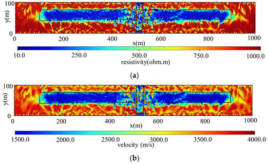
Joint inversion rectifies anomaly contours, suppresses smearing, eliminates spurious anomalies, and reconstructs anomaly spatial features with high fidelity, markedly outperforming single-method inversions, as shown in Figure 4.

Figure 4. Joint inversion of Model 1. (a) Joint inversion resistivity result; (b) joint inversion velocity result.

4.2. Model 2: Fractured Water-Conducting Channel

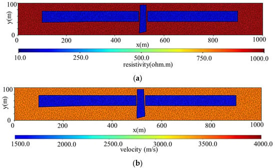
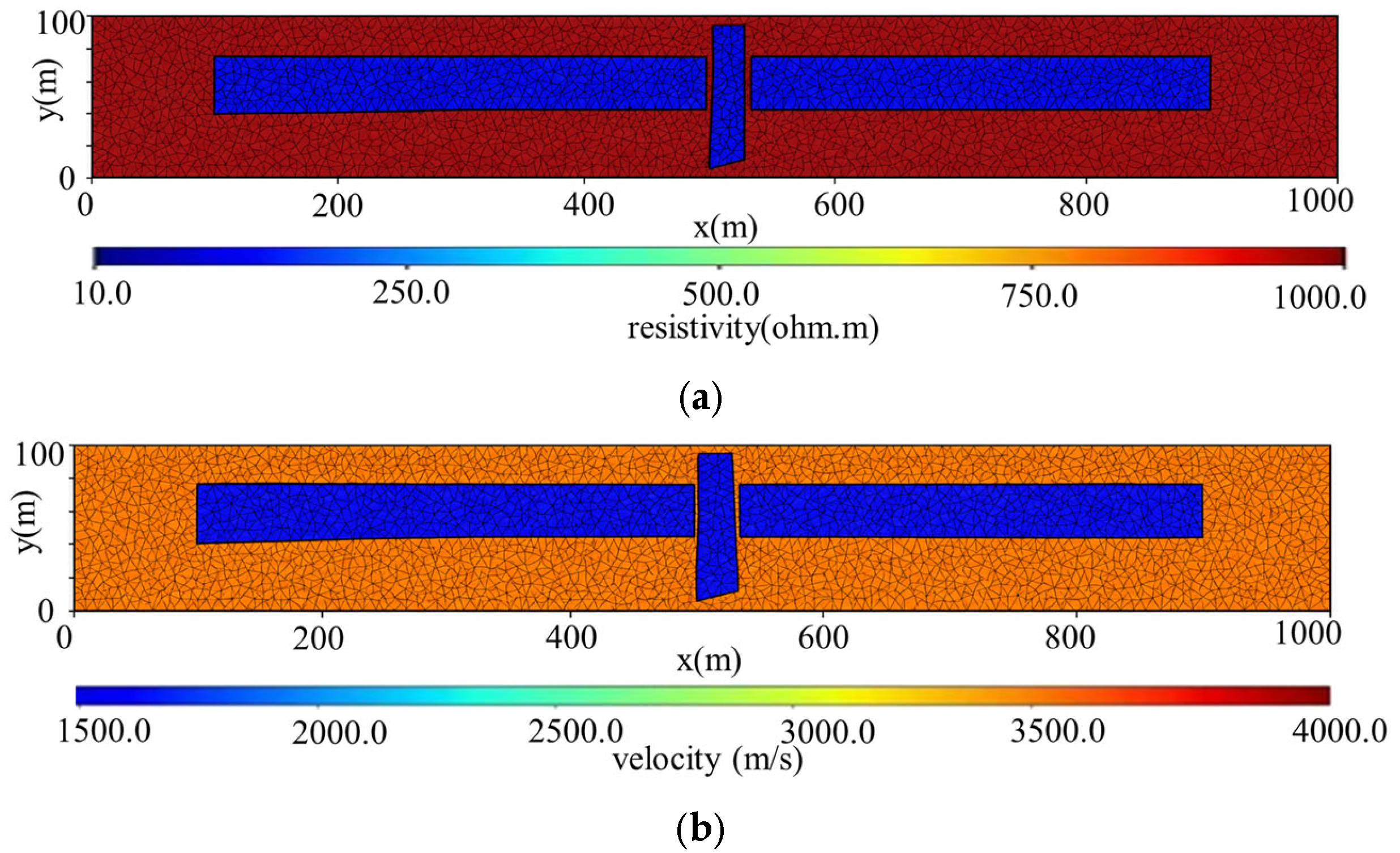
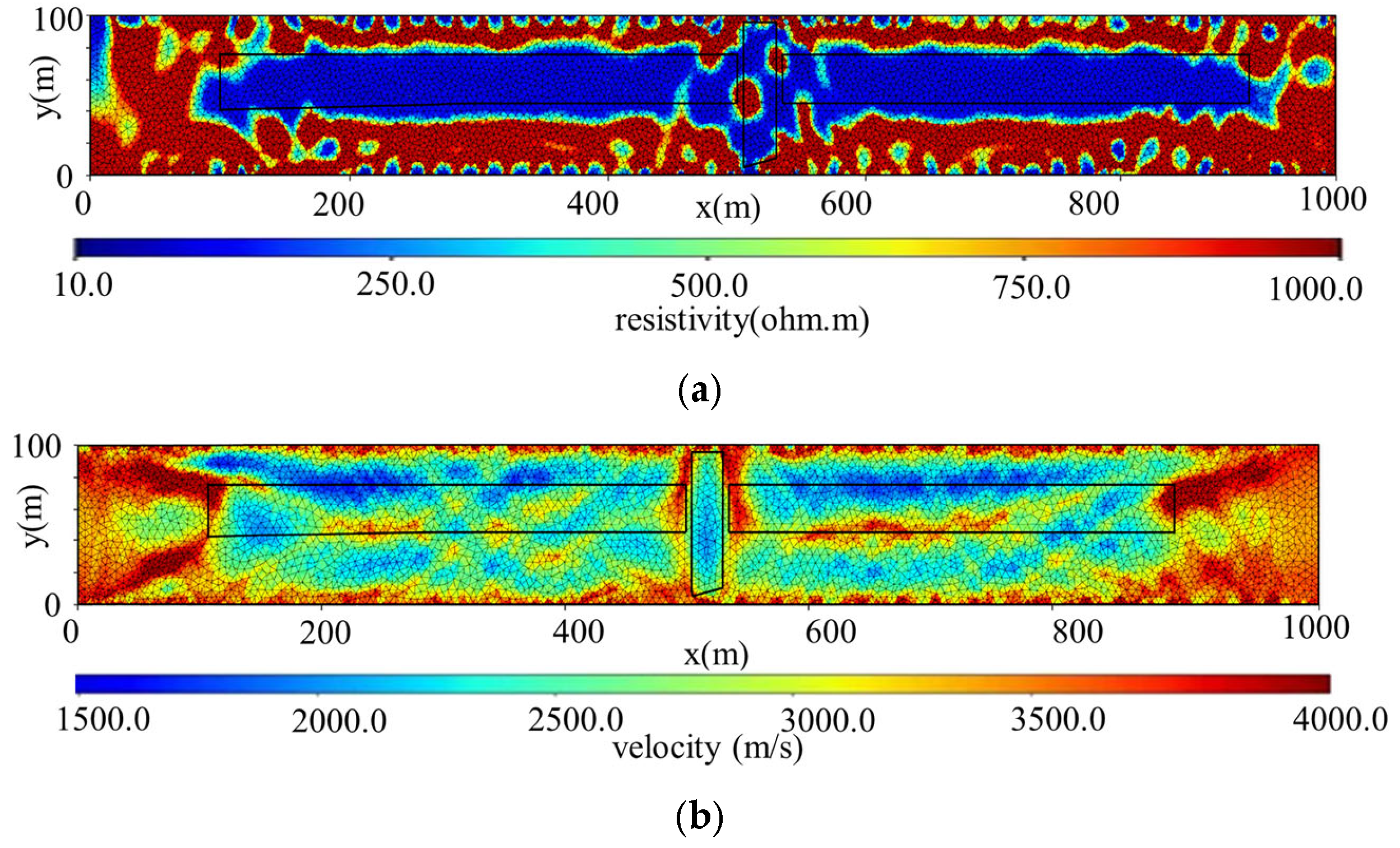
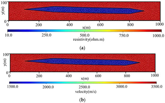
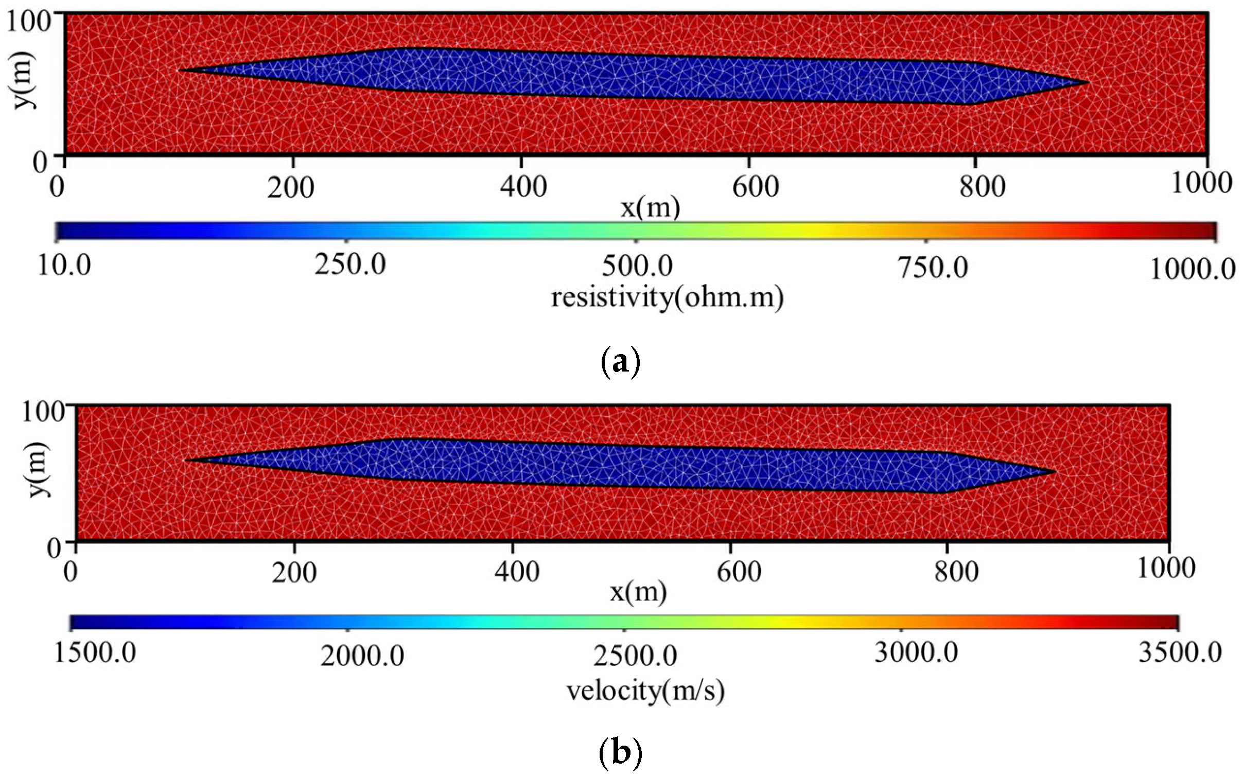
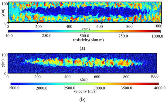
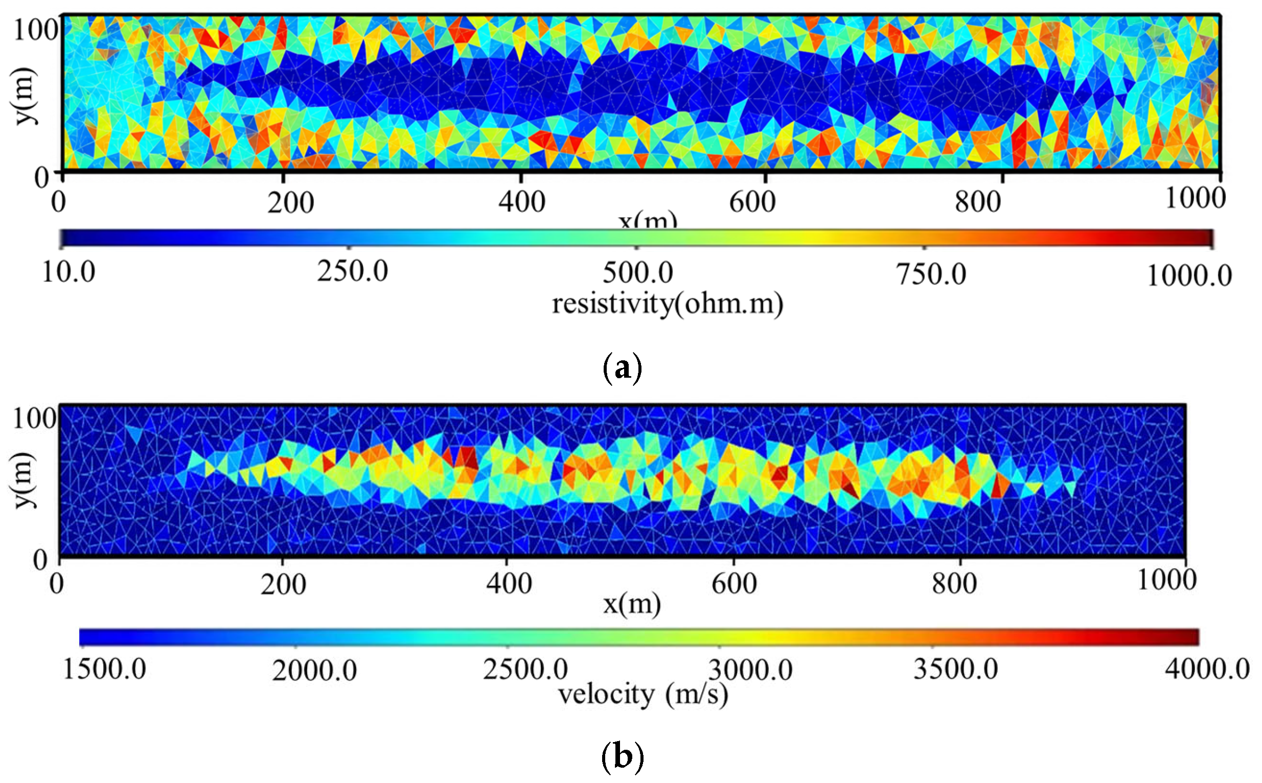
The model represents a linear water-conducting fracture, characterized by a single elongated low-resistivity anomaly and a corresponding low-velocity anomaly, as shown in Figure 5.

Figure 5. DC resistivity and seismic exploration model of Model 2. (a) Resistivity model; (b) velocity model.

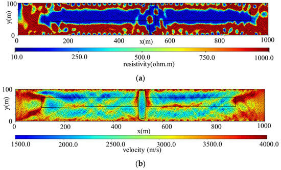
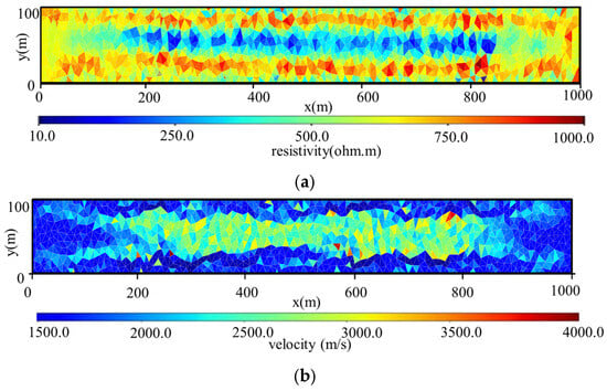
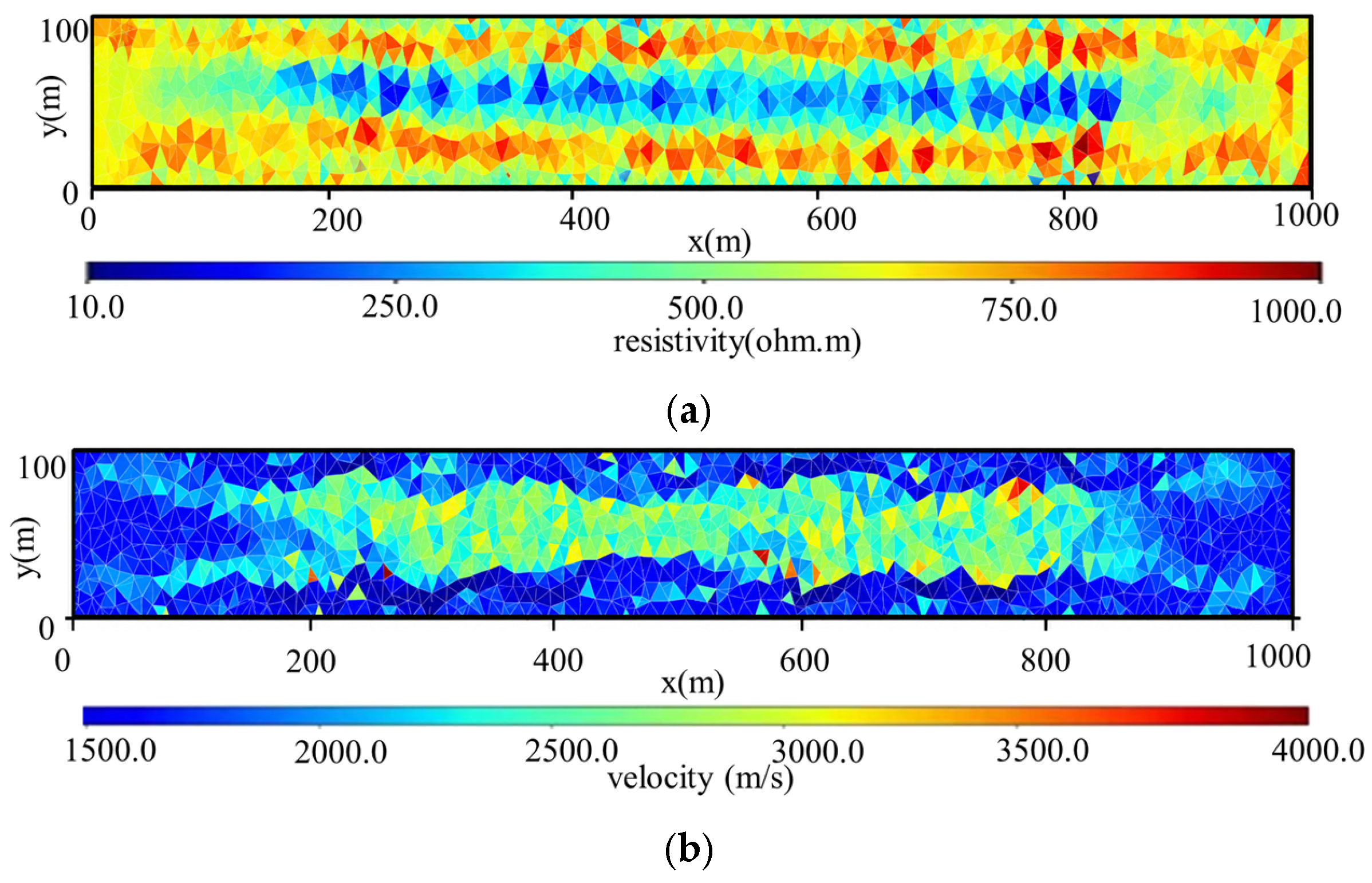
In the single resistivity inversion result, the low-resistivity anomaly appears elongated, its sharp terminations at both ends are not clearly identified, and spurious anomalies are present. In the single seismic inversion result, the sharp ends of the low-velocity anomaly are similarly not delineated accurately, as shown in Figure 6.

Figure 6. Single inversion of Model 2. (a) Single DC inversion resistivity result; (b) single seismic inversion velocity result.

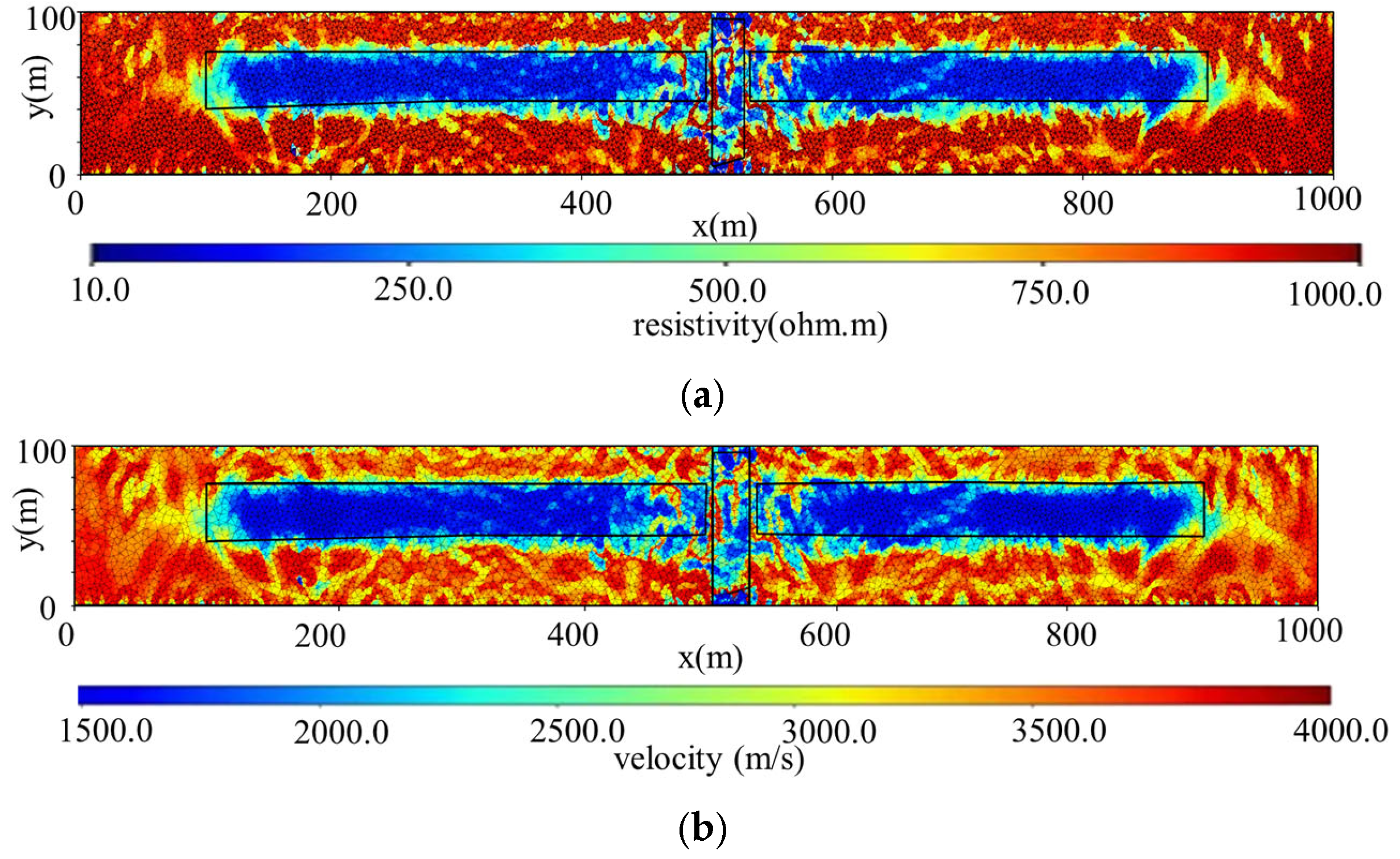
Joint inversion refines anomaly extents, accurately captures sharp channel terminations, and suppresses smearing, demonstrating high precision in imaging linear hydrogeological conduits, as shown in Figure 7.

Figure 7. Joint inversion of Model 2. (a) Joint inversion resistivity result; (b) joint inversion velocity result.

5. Discussion

5.1. Interpretation of Joint Inversion Results

The numerical experiments presented in this study demonstrate the superior performance of the seismic–electric joint inversion framework for detecting concealed hazardous structures in underground mine environments. The comparative analysis between single-method inversions and joint inversion reveals several key findings that warrant further discussion.

5.2. Novelty Elements and Method Justification

Joint inversion of multiple geophysical datasets has been extensively investigated in the literature. The pioneering work of Vozoff and Jupp [5] established the theoretical foundation for joint inversion by exploiting the interdependence between different physical properties. Subsequent studies by Lines et al. [6] and Gallardo and Meju [9] further developed cooperative and cross-gradient joint inversion approaches, respectively. The cross-gradient constraint, originally proposed by Gallardo and Meju [9] and extended to 3-D applications by Shi et al. [3], provides a structurally coupled regularization that does not require explicit petrophysical relationships between different physical parameters. In contrast to studies that assume empirical correlations (e.g., velocity–resistivity relationships based on Archie’s law or laboratory calibrations), the cross-gradient approach is data-driven and adapts to local structural consistency.

Several studies have applied joint inversion techniques to mineral exploration and subsurface imaging problems. Dell’Aversana [30] proposed a self-aware joint inversion framework that adaptively adjusts coupling parameters during the inversion process. However, these studies primarily focus on regional-scale applications with relatively simple geological settings. The application of joint inversion to complex underground mine environments, characterized by irregular roadway boundaries, localized anomalies, and heterogeneous media, remains relatively underexplored.

The present study introduces several novel elements that distinguish it from existing approaches: (1) Unstructured mesh discretization using Delaunay triangulation [22,23] enables accurate representation of complex mine geometries and roadway boundaries, which are difficult to accommodate in structured mesh formulations. This is particularly important for mine-scale applications where the survey geometry is constrained by existing underground infrastructure. (2) Curved-ray seismic tomography [22,27] provides more accurate traveltime calculations compared to straight-ray methods, especially in heterogeneous media with strong velocity contrasts. The curved-ray approach based on Fermat’s principle iteratively corrects ray trajectories to align with true wave paths, improving the reliability of velocity inversions in complex mine environments. (3) The LSQR algorithm [27,29] efficiently solves the large, sparse linear systems arising from tomographic inversions while exploiting matrix sparsity to reduce computational memory requirements and avoid numerical instabilities.

Regarding the choice of methods, we deliberately selected established techniques with proven stability and reliability rather than pursuing the most computationally advanced approaches. While more sophisticated methods such as full-waveform inversion (FWI) or neural network-based inversion exist, they require extensive computational resources, high-quality wide-bandwidth data, and careful preprocessing that may not be readily available in typical mine survey configurations. The Occam-style regularized inversion [20] used for DC resistivity provides a balanced trade-off between data misfit and model smoothness, avoiding over-fitting while maintaining reasonable resolution. Similarly, the Gauss–Newton optimization framework offers sufficient convergence speed for practical applications without the complexity of quasi-Newton or stochastic optimization methods.

5.3. Limitations and Future Work

Several limitations of the present study should be acknowledged. First, the numerical experiments are based on synthetic data with known ground truth, which may not fully capture the complexities of real field data, including measurement noise, instrument response, and environmental effects. Second, the study focuses on 2-D cross-section models, while actual underground mine environments are inherently three-dimensional. Future work will extend the proposed framework to 3-D joint inversion with unstructured tetrahedral meshes. Third, the current study does not account for petrophysical variability within anomalous bodies; incorporating laboratory-derived or in situ measured petrophysical relationships could further improve the quantitative interpretation of inversion results. Validation through field case studies at operational mine sites is planned as the next step to demonstrate the practical applicability of the proposed methodology.

6. Conclusions

This study addresses the limitations of low resolution and high non-uniqueness inherent in single geophysical methods for detecting concealed hazardous structures in underground mines. By combining theoretical derivation, algorithm development, and numerical validation, we establish a comprehensive seismic–electric joint inversion framework. The main conclusions are summarized as follows.

(1)

Single-method inversion frameworks tailored to mining conditions have been developed. For the DC resistivity method, we couple unstructured-mesh finite-element forward modeling with Occam-style regularized inversion, which reliably reconstructs the positions and resistivity parameters of anomalous bodies. For the seismic method, we adopt curved-ray forward modeling combined with the LSQR algorithm, which accurately images velocity anomalies. These frameworks lay a solid foundation for the subsequent joint inversion.

(2)

A cross-gradient-constrained seismic–electric joint inversion scheme has been formulated. The scheme unifies the data-fitting term, regularization term, and cross-gradient term within a single objective function. By enforcing structural consistency between the resistivity and velocity models without assuming any empirical petrophysical relationship, the proposed scheme effectively suppresses spurious anomalies and image smearing, thereby improving the reliability of the inverted solutions.

(3)

The effectiveness of the joint inversion has been verified through numerical experiments on representative mining scenarios, including multiple isolated anomalies, fractured water-conducting channels, and water-bearing faults. Compared with the single-method inversions, the proposed approach substantially improves the morphological reconstruction of anomalies, eliminates spurious features, and reduces solution non-uniqueness, offering a practical tool for the precise detection of concealed hazard-inducing structures in coal mines.

(4)

The results and innovations presented in this study benefit multiple stakeholder groups in the mining industry, including mine safety engineers, geophysical surveyors, mining geologists, and mine management personnel. The proposed seismic–electric joint inversion framework provides these professionals with a robust and reliable tool for detecting concealed hazardous structures, thereby enhancing the safety and efficiency of underground mining operations. In day-to-day mining practice, the methodology can be integrated into routine geophysical monitoring programs for mine water inrush prediction, fractured zone characterization, and advanced detection of water-bearing structures ahead of the working face. The improved imaging accuracy of anomalous bodies enables proactive hazard mitigation, reducing the risk of water inrush accidents and associated economic losses. Moreover, the unstructured mesh discretization technique accommodates complex mine geometries and roadway boundaries, making the method particularly suitable for practical mine survey configurations. The practical applicability of the proposed framework has been demonstrated through numerical experiments, and future work will focus on field validation through data acquisition at operational mine sites to further bridge the gap between numerical simulations and real-world applications.

References

- Luo, B.; Sun, Y.; Xu, Z.; Chen, G.; Zhang, L.; Lu, W.; Zhao, X.; Yuan, H. Damage Characteristics and Mechanism of the 2017 Groundwater Inrush Accident That Occurred at Dongyu Coalmine in Taiyuan, Shanxi, China. Water 2021, 13, 368. [Google Scholar] [CrossRef] [Scilit]
- Li, A.; Ding, X.; Yu, Z.; Wang, M.; Zhang, B.; Han, T.; Mu, Q.; Dai, Z.; Li, H. Prediction Model of Fracture Depth and Water Inrush Risk Zoning in Deep Mining Coal Seam Floor. Environ. Earth Sci. 2022, 81, 315. [Google Scholar] [CrossRef] [Scilit]
- Shi, Z.; Hobbs, R.W.; Moorkamp, M.; Tian, G.; Jiang, L. 3-D Cross-Gradient Joint Inversion of Seismic Refraction and DC Resistivity Data. J. Appl. Geophys. 2017, 135, 31–43. [Google Scholar] [CrossRef] [Scilit]
- Hong, W.; Sheng, W. A DEMATEL-ISM-BN Model of Mine Water Inrush Accidents. Mine Water Environ. 2023, 42, 178–186. [Google Scholar] [CrossRef] [Scilit]
- Vozoff, K.; Jupp, D.L.B. Joint Inversion of Geophysical Data. Geophys. J. R. Astron. Soc. 1975, 42, 977–991. [Google Scholar] [CrossRef] [Scilit]
- Lines, L.R.; Schultz, A.K.; Treitel, S. Cooperative inversion of geophysical data. Geophysics 1988, 53, 8–20. [Google Scholar] [CrossRef] [Scilit]
- Hering, A.; Misiek, R.; Gyulai, A.; Ormos, T.; Dobrola, M.; Dresen, L. A joint in-version algorithm to process geoelectric and surface wave seismic data. Part I: Basic ideas1. Geophys. Prospect. 1995, 43, 135–156. [Google Scholar] [CrossRef] [Scilit]
- Kis, M.; Gyulai, A.; Ormos, T.; Dobróka, M. Joint inversion of Love and Rayleigh wave group velocities, re-fraction traveltimes and DC apparent resistivities measured above 2D geological structures. Publ. Univ. Miskolc Ser. A Min. Geotechnol. 2001, 59, 23–38. [Google Scholar]
- Gallardo, L.A.; Meju, M.A. Characterization of heterogeneous near-surface materials by joint 2D inversion of dc resistivity and seismic data. Geophys. Res. Lett. 2003, 30, 1658. [Google Scholar] [CrossRef] [Scilit]
- Yu, P.; Zhang, L.; Wang, J.; Wu, J. Determination of Physical Property Parameters Structure in Middle Guizhou Uplift by Joint Inversion of Magnetotelluric, Seismic, Gravity and Magnetic Data. J. Tongji Univ. Nat. Sci. 2008, 36, 406–412. [Google Scholar]
- Chen, X.; Yu, P.; Zhang, L.-L.; Li, Y.; Wang, J.-L. Adaptive regularized synchronous joint inversion of MT and seismic data. Chin. J. Geophys. 2011, 54, 2673–2681. (In Chinese) [Google Scholar] [CrossRef]
- Zhou, L. Two Dimensional Joint Inversion of MT and Seismic Data. Master’s Thesis, China University of Geo-Sciences, Beijing, China, 2012. [Google Scholar]
- Gao, J.; Zhang, H.-J. Two-dimensional joint inversion of seismic velocity and electrical resistivity using seismic travel times and full channel electrical measurements based on alternating cross-gradient structural constraint. Chin. J. Geophys. 2016, 59, 4310–4322. (In Chinese) [Google Scholar] [CrossRef]
- Peng, M.; Tan, H.-D.; Jiang, M.; Qian, H.; Tan, J.-Y. Three-dimensional joint inversion of magnetotelluric and seismic travel time data with cross-gradient constraints. Chin. J. Geophys. 2013, 56, 2728–2738. (In Chinese) [Google Scholar] [CrossRef]
- Wang, Z.; Wang, C.; Fang, S.-N. Constraint inversion of three-dimensional bore-hole-to-surface resistivity based on unstructured finite element. Geophys. Geochem. Explor. 2022, 46, 1431–1443. [Google Scholar] [CrossRef]
- Wu, X.-P.; Xu, G.-M. Study On 3-D Resistivity Inversion Using Conjugate Gradient Method. Chin. J. Geophys. 2000, 43, 420–427. (In Chinese) [Google Scholar] [CrossRef] [Scilit]
- Saad, Y. Iterative Methods for Sparse Linear Systems, 2nd ed.; SIAM: Philadelphia, PA, USA, 2003. [Google Scholar]
- Haber, E.; Oldenburg, D.W. Joint inversion: A structural approach. Inverse Probl. 1997, 13, 63–77. [Google Scholar] [CrossRef] [Scilit]
- Tang, J.T.; Wang, F.Y.; Ren, Z.Y. 2.5-D DC Resistivity Modeling by Adaptive Finite-Element Method with Unstructured Triangulation. Chin. J. Geophys. 2010, 53, 708–716. [Google Scholar] [CrossRef]
- Constable, S.C.; Parker, R.L.; Constable, C.G. Occam’s Inversion: A Practical Algorithm for Generating Smooth Models from Electromagnetic Sounding Data. Geophysics 1987, 52, 289–300. [Google Scholar] [CrossRef] [Scilit]
- Wang, Y.F.; Yagola, A.G.; Yang, C.C. Optimization and Regularization for Computational Inverse Problems and Applications; Higher Education Press: Beijing, China, 2010. [Google Scholar]
- Greenhalgh, S.A.; King, D.W. Curved raypath interpretation of seismic refraction data. Geophys. Prospect. 1981, 29, 853–882. [Google Scholar] [CrossRef] [Scilit]
- Shewchuk, J.R. Delaunay Refinement Algorithms for Triangular Mesh Generation. Comput. Geom. 2002, 22, 21–74. [Google Scholar] [CrossRef] [Scilit]
- Wang, X.L.; Li, Y.H.; Wang, P.; Wang, X.Y.; Lü, M.H. Estimation and application of micro-seismic data SRV based on improved Delaunay triangulation algorithm. Prog. Geo-Phys. 2021, 36, 689–695. [Google Scholar] [CrossRef]
- Zhao, B.; Meng, X.; Hou, J. Building and Visualization of 3D Seismic Model. Earth Sci. 2007, 32, 549–553. [Google Scholar]
- Thurber, C.H.; Ellsworth, W.L. Rapid solution of ray tracing problems in heterogeneous media. Bulle-Tin Seismol. Soc. Am. 1980, 70, 1137–1148. [Google Scholar] [CrossRef] [Scilit]
- Paige, C.C.; Saunders, M.A. LSQR: An Algorithm for Sparse Linear Equations and Sparse Least Squares. ACM Trans. Math. Softw. 1982, 8, 43–71. [Google Scholar] [CrossRef] [Scilit]
- Lee, E.J.; Huang, H.; Dennis, J.M.; Chen, P.; Wang, L. An optimized parallel LSQR algorithm for seismic tomography. Comput. Geosci. 2013, 61, 184–197. [Google Scholar] [CrossRef] [Scilit]
- Nolet, G. Solving or Resolving Inadequate and Noisy Tomographic Systems. J. Comput. Phys. 1985, 61, 463–469. [Google Scholar] [CrossRef] [Scilit]
- Liu, J. Research on Synchronous Geophysical Joint Inversion. Master’s Thesis, East China University of Technology, Nanchang, China, 2023. [Google Scholar] [CrossRef]
- Dell’ Aversana, P. Self-Aware Joint Inversion of Multidisciplinary Geophysical Data in Mineral Exploration Using Hyperparameter Self-Adjustment: A Preliminary Study. Minerals 2025, 15, 623. [Google Scholar] [CrossRef] [Scilit]
Disclaimer/Publisher’s Note: The statements, opinions and data contained in all publications are solely those of the individual author(s) and contributor(s) and not of MDPI and/or the editor(s). MDPI and/or the editor(s) disclaim responsibility for any injury to people or property resulting from any ideas, methods, instructions or products referred to in the content. |
© 2026 by the authors. Licensee MDPI, Basel, Switzerland. This article is an open access article distributed under the terms and conditions of the Creative Commons Attribution (CC BY) license.