


Featured Application
This study provides theoretical insight into how membrane-associated silica-coated magnetic nanoparticles may transiently alter local electroporation conditions, offering a basis for future experimental investigations of nanoparticle–electroporation interactions.
Abstract
Electroporation outcomes are governed by the local electric field distribution and transmembrane voltage, both of which may be altered by nanoscale elements positioned near the cell membrane. In this study, we developed a two-dimensional finite-element electromagnetic model to investigate the effect of a membrane-proximal silica-coated superparamagnetic iron oxide nanoparticle cluster during a trapezoidal electroporation pulse. The model couples electric and magnetic field components with a membrane electroporation formulation based on Smoluchowski-type pore-density dynamics. Simulations were performed with and without a nanoparticle positioned 5 nm from the membrane, considering different cytosol and extracellular medium conductivities. The results show that the nanoparticle induces a highly localized perturbation of the electric field, whose magnitude depends on the sampling region and conductivity contrast. Transmembrane voltage is modestly and transiently modulated during pulse rise time, whereas the effect is limited during the pulse plateau. Pore-density analysis further indicates that the nanoparticle does not induce a generalized increase in electroporation-related parameters and may locally reduce pore density near the nanoparticle–membrane interface. Overall, the model identifies transient and conductivity-dependent nanoscale field redistribution caused by membrane-proximal silica-coated magnetic nanoparticles, while highlighting the need for three-dimensional modeling and experimental validation before inferring electroporation enhancement.
1. Introduction
Cell electroporation can be exploited in clinical treatments to improve the permeability of biological cell membranes and deliver molecules like chemotherapy agents or genes [1,2,3,4,5,6]. This physical modality uses sequences of nominally rectangular but physically trapezoidal voltage pulses, due to finite rise and fall times, to generate locally an electric field able to rearrange temporarily the cell membrane and open aqueous pores able to improve cellular uptake [2,5,7]. It is well known that electric field distribution depends on electric properties of materials and at the macroscopic level, some analyses are presented in [8,9,10,11,12,13,14,15]. Moreover, some authors investigated membrane-related phenomena on a tissue scale using numerical models [14,16,17,18,19]. The use of nanoparticles has multiple potential applications in medicine, such as drug vectors, hyperthermia agents, internal electrodes or in immunotherapy [20,21,22,23,24,25,26,27,28,29,30,31]. In previous studies, various nanoparticle (NP) functionalization strategies have been developed to improve their accumulation within specific organs or tissues. Such approaches have been extensively explored for applications including magnetic fluid hyperthermia, magnetic resonance imaging (MRI) contrast enhancement, and targeted drug delivery systems based on magnetic nanoparticles [20,24,30,32,33,34,35,36,37,38,39]. In addition, several studies have proposed the use of externally applied magnetic fields to actively guide magnetic nanoparticles toward predefined anatomical targets, thereby improving spatial targeting and local accumulation at the desired site [27,40,41,42]. In this paper, the NPs are investigated as perturbation elements of the electric field distribution, once they have reached the proximity of a cell membrane.
In order to improve electroporation without increasing the external electric field, Lekner [43] proposed the use of small conducting objects (micro-conductors) to locally enhance the electric field distribution in the tumor area, where the micro-conductors are injected and external electric pulses are applied.
To study the influence of small objects, namely the nanoparticles, the electromagnetic problem has to be studied at the cell level, as in [44,45,46,47]. The influence of conductive nanoparticles was theorized by using numerical simulations. For instance, Lekner predicted the enhancement of electroporation in the presence of microelectrodes made of conductive prolate [43], which could, according to simulations developed therein, enhance the external electric field up to 100 times. Such an amplification was noted for prolate structures with an aspect ratio of 15.7, when aligned with the lines of the electric field. Conversely, the electric field on the surface of conducting spheres could be amplified three times the external field [43]. Indeed, in the quest to attain this attractive phenomenon, experiments have been performed by several research groups. Authors generally reported a limited effect of tested spherical and rod-shaped gold nanoparticles for electroporation enhancement. Even in the case of gold nanospheres, the predicted three-times field amplification was never observed experimentally. Interestingly, in some reports [48,49,50,51], a marginal improvement of electroporation was achieved.
Importantly, as also noted by Lekner [43], the field strength rapidly decreases with increasing distance from either pole of the conducting prolate or the surface of the conducting sphere. Therefore, some groups have proposed the use of magnetic structures, which can be magnetically oriented and concentrated in close proximity to cellular membranes with the use of an external magnetic field gradient. Such structures could be used as internal electrodes acting as transducers of an external time-varying magnetic field [22,25]. However, it is important to note that, in order to translationally move along a magnetic field gradient and thus be effectively magnetically guidable, single-core superparamagnetic nanoparticles generally possess insufficient magnetic moment. Conversely, multicore assemblies exhibit markedly enhanced magnetic moments and hence also magnetic responsiveness and translational movement ability.
Within this perspective, the effect on electric field distribution and transmembrane voltage in a region around the cell membrane in the presence of a silica-coated multicore magnetic nanoparticle is investigated. Such nanoparticles, namely the silica-coated superparamagnetic iron oxide nanoparticle (SPION) clusters [52], were considered because of their excellent magnetic responsiveness. The assembled nanoparticles cluster is spherical and can be considered as one nanostructured entity, namely one magnetic nanoparticle (NP) [20]. Such clusters preserve the superparamagnetic properties [20] and could be first guided to the proximity of a cell membrane. Once attracted to the site of interest (namely, the proximity of a cell membrane), the external magnetic field could be removed, and electric pulses could be applied.
To solve the electromagnetic problem and compute the transmembrane potential, among the different possible numerical approaches proposed in the literature (see, for example, [12,16,19,45,53,54,55,56]), a transient problem was considered in this contribution, as suggested in [12,14,57]. In order to account for the electroporation phenomenon, the morphological modification of the cell membrane due to electrically induced pores is herein modeled by introducing a current density source on the membrane domain. Such current, governed by the Smoluchowski approximation of the pore-density dynamic Np(t), introduces a new differential equation that has to be solved together with the Maxwell equation on the membrane. The idea is to analyze the effect of the transient phase of the voltage pulse on the electric field distribution near the cell membrane in the absence and presence of a nanoparticle, considering also the magnetic field component. In particular, the effect of an electric field, due to a trapezoidal-shaped voltage pulse with a predefined rise time (i.e., the transient part of the pulse before the plateau) applied to the system, was analyzed at different time instants, belonging to the rise time interval and to the pulse plateau. In this way, the transient effect occurring during the voltage pulse rise from 0 V to the plateau value is investigated by solving the coupled electromagnetic problem and electroporation phenomenon in the time domain.
2. Materials and Methods
2.1. Numerical Problem
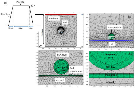
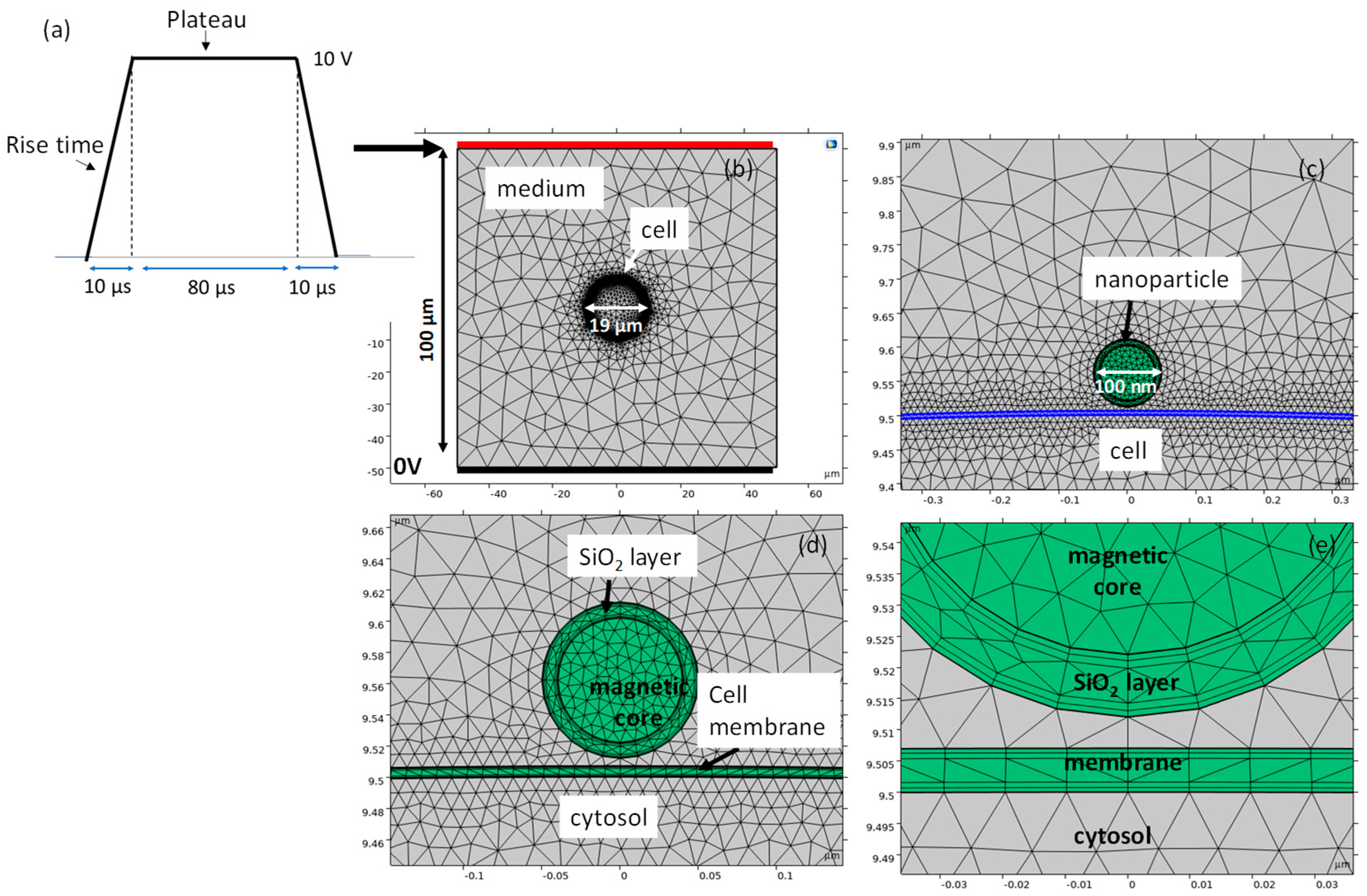
The 2D section of the problem geometry is represented in Figure 1. A square box with a side length of 100 μm represents the box where a circular section of a spherical cell is positioned in the center (Figure 1a). In general, this 2D geometry is used in the microscopic scale evaluation [45,58,59,60,61]. The cell diameter in the proposed geometry is 19 μm (radius 9.5 μm) with a membrane thickness of 7 nm. The cell membrane, a bilayer of phospholipid molecules, is made of a lossy dielectric material. Outside the cell membrane, the medium is represented with constant electrical conductivity. Close to the cell membrane, a silica-coated NP is positioned, and corresponding details are represented in Figure 1d–e. Nanoparticles have a magnetic core with a diameter of ~80 nm and are covered with a ~10 nm-thick silica layer with a total nanoparticle diameter of ~100 nm. A NP distance-cell membrane of 5 nm was considered herein.
Figure 1.
Geometry with mesh details and voltage pulse applied to the domain boundary: (a) applied voltage pulse, (b) geometry and mesh of the entire domain with cell geometrical details, (c) NP and cell membrane relative positioning, (d) zoom around the NP showing its composition and (e) detail of the membrane and NP regions.
Figure 1 also shows the details of the mesh of the geometry at different scales, from the overall domain to the one at the smallest scale, showing the cell membrane and silica coating of the magnetic nanoparticle. The thin domain included a layered mesh with 3 rectangular elements per layer close to the domain boundary. The typical mesh has 180,000 domain elements and 100,000 vertex elements, leading to a quite complex numerical problem. The thin silica shell was modeled as a meshed physical domain with silica properties reported in Table 1.
Table 1.
Electric properties of the materials; [NU] = no unit, NP = nanoparticle.
Typical electric properties of the material, including electrical conductivity, relative dielectric permittivity and relative magnetic permeability, are reported in Table 1. In particular, cytosol, depending on cell type, can range between 0.1 and 1 S/m and relative dielectric permittivity εr = ε/ε0 ε0 = 8.854 × 10⁻¹² F/m; the absolute permittivity of the free space can vary between 80 and 150 [53,54,58,62,63,64,65]. The typical membrane conductivity is in the order of 10−5–10−7 S/m and was fixed here to 5.6 × 10⁻⁵ S/m with a relative permittivity close to 10 [25,58,66,67]. Depending on its composition, cell culture media can have an electric conductivity ranging between 0.2 S/m and 1.5 S/m, with a relative dielectric- permittivity close to that of water, i.e., 80 [60,67,68]. Finally, the electrical properties of NPs have been selected according to the data reported in [22,69,70,71].
2.2. Magnetic and Electric Problem
In the geometry in Figure 1, the electric and magnetic field problems are solved using Finite Element Analysis (FEA) to compute electric field distribution in the domain due to the application of one electroporation pulse and considering the pore formation on the cell membrane. In particular, a trapezoidal-shaped pulse 100 μs long with not-null rise and fall time fixed to 10 μs is considered and adopted in accordance with the typical values provided by existing clinical electroporators, such as the one manufactured by Igea (Igea S.p.A. Carpi, Modena, Italy) [72,73,74]. The proposed model is used to predict the effect of magnetic NPs outside the cell membrane. Considering both the electric and magnetic field in the dielectric material, the field problem is solved in the magnetic vector potential A, and electric scalar potential, V, by the A-V formulation using Comsol Multyphysics AC/DC module (https://www.comsol.com, COMSOL AB, Stockholm, Sweden [last access 5 July 2026]) software tool [12,75,76,77]:
with
in which the electric field value E and the electric displacement field D are derived from
where µ is the permeability of the material, σ is the material conductivity and ε is the electric permittivity of the medium, in which the problem is solved. The uniqueness of the magnetic vector potential was ensured by imposing the Coulomb gauge:
Substituting Equations (2) and (3) into Equation (1), the following Ampère’s law equation was solved:
given the current-continuity equation:
It has to be noted that the corresponding total current density in Equation (2) was evaluated as the sum of conduction (i.e., ) and displacement (i.e., = ) current densities.
The Dirichlet conditions are imposed at the electrodes. On the bottom electrode, a 0 V potential was fixed and the faced electrode was energized by the voltage pulse with a plateau potential of 10 V. This way, a nominal electric field of 1000 V/cm is generated between 100 µm distance electrodes, considering here the vacuum or the presence of an homogenous dielectric medium. Moreover, Neumann conditions apply on external boundaries of the square sides that are not electrodes. Initial conditions correspond to zero field in the whole domain, except in the cell interior, for which a potential of −20 mV, named resting potential, is imposed. In fact, the potential in the cell interior is not null.
It is expected that displacement current contribution affects the problem solution in the transient phase of the pulse, in the rise and fall time interval, while a constant current solution in the constant plateau part of the pulse should be prevalent.
It is worth noting that the present study uses a two-dimensional planar model to represent the real three-dimensional cell–nanoparticle system. This approximation allows the local interaction between the nanoparticle, the extracellular medium, the membrane, and the cytosol to be investigated with sufficiently high spatial resolution, particularly in the nanometric membrane and silica-shell regions. However, the electric field perturbation generated by a finite spherical nanoparticle in 3D exhibits a different spatial decay from that obtained in a 2D cross-sectional model. Consequently, the present results should be considered primarily as a comparative analysis of the trends associated with different configurations with and without the nanoparticle, rather than as direct quantitative predictions of the full three-dimensional system.
2.3. Membrane Electroporation: Smoluchowski Solution for Membrane Conductivity
The electroporation of the cell membrane can be modeled as a multiphysics problem that merges the electromagnetic problem with the morphological modifications of a phospholipidic bilayer due to a strong electric field. By considering the asymptotic approximation of the Smoluchowski equation for electroporation that describes the time evolution of the pore population density of transient aqueous pores due to an externally applied electric field [13,45,59,78,79] at the cell membrane domain, a current density contribution, is considered:
This current density vector is directly dependent on the pore density, i.e., the number of pores per unit of surface area th, which appear on the cell membrane in case of electroporation phenomenon onset, and the current in a single pore of a fixed radius, iep. The current density acts as an increment of the membrane current at a point P along the membrane that reflects in a local, time-varying and nonlinear increase in the membrane electrical conductivity. This current also induces a lowering of the electric potential in the cell membrane electroporated area, being a current directed towards the cell center according to the unit vector ir.
By defining the transmembrane voltage (TMV) as the difference between the electric potential evaluated on the external membrane boundary, Vext, and on the internal membrane boundary, Vint:
The pore density in a point P along the cell membrane can be expressed as a function of Vm and computed, solving the following ordinary differential equation in the case of a fixed pore radius, rp (fixed to 0.79 nm):
where Np0 is the equilibrium pore density, g the electroporation coefficient, and Vep the characteristic voltage for electroporation. The current iep is given by:
where is the energy barrier inside the pore, h the thickness of the membrane, σ the conductivity of the aqueous solution inside the pore, q the electron charge, T the absolute temperature, and k the Boltzmann constant; n is the relative size of the entrance region of the pore and rp is the pore radius [78]. The values of parameters for Equations (8) and (9) are in Table 2.
Table 2.
Parameters of the pore model. NU = Not Unit.
A single effective time-dependent density (i.e., N(t)) with a fixed pore radius is often used in the literature [80,81]. This is a mathematical simplification that helps to reduce the problem complexity. It is well known that this is an approximation that ignores the physical reality that pore sizes may fluctuate and grow, leading to larger pores in regions exposed to high electric fields [82]. This phenomenon is not accounted for here, and all evolving defects are considered at a set represented by the thermodynamic equilibrium value (here assumed 0.79 nm). Then, the additional pores opened on the cell membrane contribute with an additional current component and here, Jtot of Equation (2) becomes
As a consequence, on the membrane domain, a multiphysics problem is established and has to be solved in the three variables: vector potential A, electric potential V and density of pores Np.
While the Smoluchowski equation used to calculate pore density is highly temperature-dependent, the temperature rise in our system can be considered neglectable. Precisely, given the volume fraction of nanoparticles with respect to the medium, the heating would only stem from the properties of the medium, and would not exceed 0.3 °C (for the highest conductivity medium). The reported temperature estimate concerns bulk heating only and does not address possible nanoscale interfacial temperature gradients. In fact, even if the 100 nm NP is potentially a heating source, the volume in which it is inserted attenuates any appreciable heating effect.
2.4. Computation Problem
The proposed simulation approach is based on a continuum/effective model. The nanoparticles are not described at the atomistic scale; instead, their electromagnetic effects are introduced through effective material properties. This modeling strategy is consistent with the approach adopted in several previous scientific works dealing with nanoparticle-mediated electroporation, where FEM-based models have been successfully used to describe the macroscopic field distribution and the resulting response of systems containing nanoscale inclusions [22,47,48,62]. All these models are well established and all based on the one previously developed for FEA by Krassakowa et al. [45,59] to study electroporation effects, for instance, the ones proposed by [18,44,58,60,66].
The numerical problem was solved using the A-V formulation according to the equations defined in Section 2.2 in all domains except the membrane, where the equations of Section 2.3 are considered, including the Np variable also. In order to investigate the effect of different medium conductivities jointly with NP influence, the study is conducted by changing the cytosol, σc, and cell culture media, σcm, conductivities in the two main cases, with and without the NP. In particular, fixing the problem geometry (NP-membrane distance 5 nm, NP diameter 100 nm, silica layer thickness 5 nm) as described in the model section, the pulse rise time (fixed to 10 µs) and pulse length (fixed to 100 µs), the following combinations of electrical conductivities were analyzed:
- σc = 0.1 Sm−1 and σcm = 0.2 Sm−1
- σc = 1 Sm−1 and σcm = 0.2 Sm−1
- σc = 0.1 Sm−1 and σcm = 1.34 Sm−1
- σc = 1 Sm−1 and σcm = 1.34 Sm−1
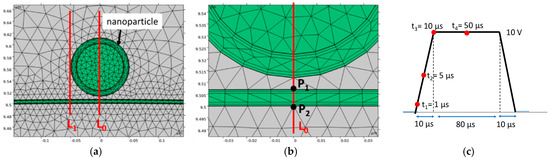
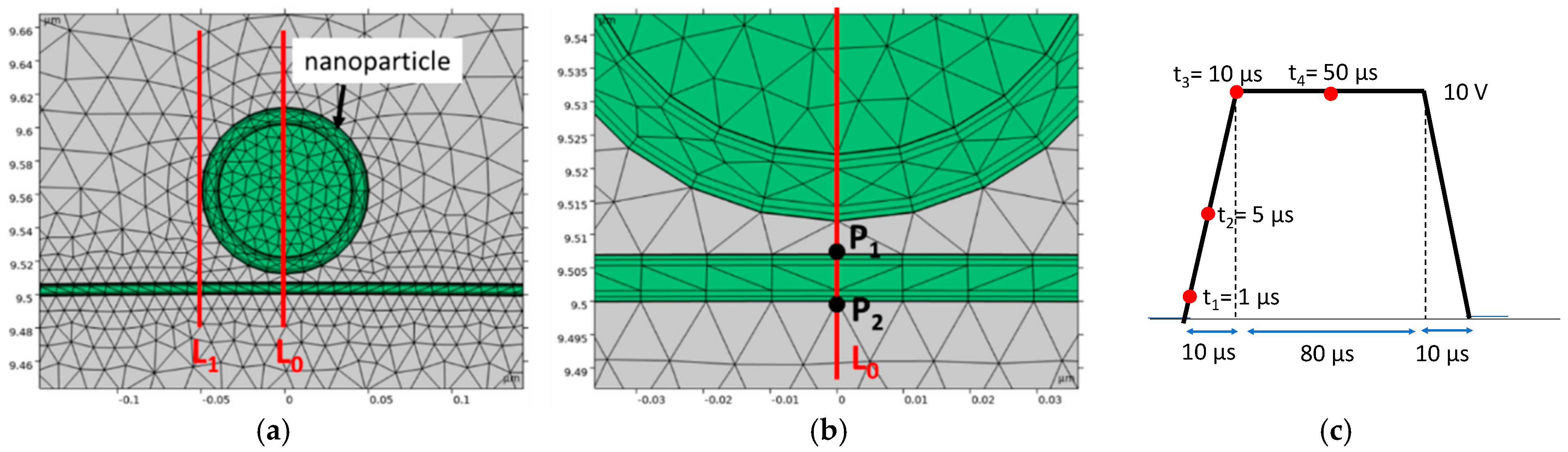
For each combination of parameters, the electric field strength E, the potential V along a line, and the TMV on the membrane domain were evaluated. The electric field strength and the electric potential are sampled along the two red lines represented in Figure 2a, labeled L0 and L1, and evaluated at the four-time instants marked by red points in Figure 2c. These time instants are located during the rise time (t1, t2 and t3), where the displacement current component superposed to the conduction component is expected, and during the pulse plateau (t4), where the conduction current should be prevalent, whereas the displacement current is expected to be negligible. The TMV is evaluated, at the same time instants, on the boundary of the cell membrane region as the difference between the electric potential in the internal and the external membrane boundary.
Figure 2.
(a) Detail of the NP Region Of Interest (ROI), where the red line shows the sampling domain for the electric field strength and potential; (b) detail of the NP-cell membrane region with the point P1 and P2 used to compare the electric field strength and potential in the parametric analysis; (c) time instants at which the analysis is conducted.
The conduction and displacement current maps and those concerning the electric field were visualized at the four time instants for all configurations in the region close to the nanoparticle and compared with those obtained without the nanoparticle.
Finally, the electric field and electric potential in the two main cases, with and without the NP, for all the configurations were compared at the point P1 and P2 marked in Figure 2b in order to evaluate the effect in the cell membrane region close to the NP.
A mesh sensitivity analysis was performed by comparing three meshes with different levels of discretization: a coarse mesh, the one adopted in presented simulations, and a refined mesh. The quantities of interest, namely the electric field in 10 points located in the region of the NP and cell membrane at some representative time instants, varied by less than 0.7% between the adopted one, with 185,944 elements (24,600 in the thin regions), and refined meshes, with 318,444 elements (49,232 in the thin regions). Therefore, the adopted mesh was considered sufficient for the present parametric study.
2.5. Magnetic Nanoparticles
The modeled magnetic nanoparticles correspond to silica-encapsulated SPION clusters, which are commercially available from Nanos Scientificae Ltd. (Nanos SCI, Ljubljana, Slovenia). These structures are synthesized in a microemulsion, where a large number of maghemite nanoparticles (γ-Fe2O3; size ~10 nm) are self-assembled into spherical nanoparticle clusters, and subsequently encapsulated with a layer of silica, as described elsewhere [83]. The nanoparticle cluster size is subsequently unified by high-gradient magnetic separation, as described in [52]. The presented model includes the magnetic properties/permeability of the NP core, but does not simulate magnetic guidance fields. The static or dynamic external magnetic field that could be used to position the NPs was thus not included in the FEM simulation.
2.6. Magnetic Nanoparticles Properties
The magnetic properties of aqueous suspensions of NPs were characterized using a Vibrating Sample Magnetometer option of PPMS (Physical Properties Measurement System manufactured by Quantum Design) [84]. The study of the magnetization (M in (emu/cm3)) as a function of an applied external field (H in (Oe)) at room temperature was used to evaluate the relative magnetic permeability, , used in the simulations. Since M is measured in emu/cm3 and H is in Oe, is obtained as and reported in Table 1.
The magnetic nanoparticles also have a negative surface charge (with a zeta potential of −25 mV at pH = 7 [52]), which was not considered in the simulation. It is worth noting that in aqueous environments these particles develop an electric double layer, which might screen the local electric field at the nanoscale.
3. Results and Discussion
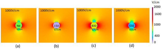
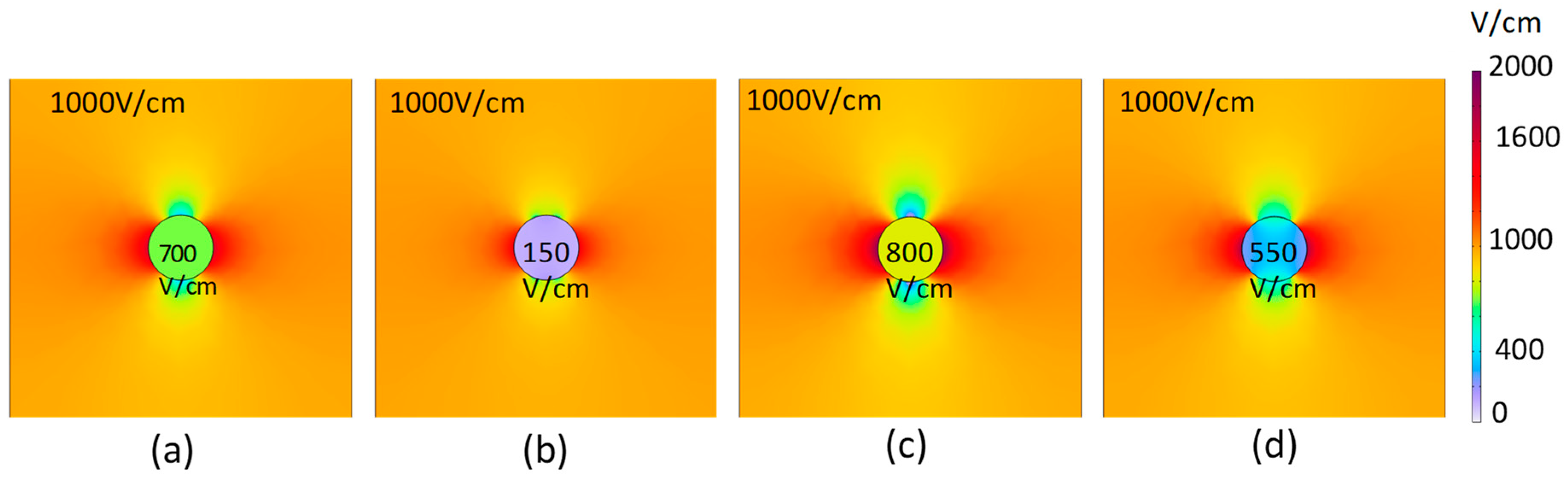
The numerical results in Figure 3 show the electric field around the cell at 50 µs and inside the cell considering the four cytosol, σc, and cell culture media, σcm, combination conductivities. Outside the cell, the electric field strength is approximately 1000 V/cm in the entire area except in proximity to the cell, where it varies between 100 and 1600 V/cm depending on media conductivities. Also, in the cell cytosol, the electric field strength assumes different values depending on the cytosol and medium conductivities and in this case, the electric field strength varies between 150 and 800 V/cm. Conversely, Figure 4 reports the electric field strength in a ROI in the proximity of the cell membrane in the absence (Figure 3a) and presence (Figure 3b) of the NP. Each figure in the panel shows the color map of the electric field strength when the cell is surrounded by a specific medium described with the corresponding electrical conductivity and can be used to compare the effect of different cell culture mediums (CCM) in the electroporation protocol (e.g., CCM of RPMI type with σ = 1.34 S/m or CCM of low conductivity (LCM) with σ = 0.2 S/m).
Figure 3.
Electric field strength in the entire model for different conductivities combinations of the cell (middle) or the pulsation medium: (a) σc = 0.1 Sm−1 and σcm = 0.2 Sm−1, (b) σc = 1 Sm−1 and σcm = 0.2 Sm−1, (c) σc = 0.1 Sm−1 and σcm = 1.34 Sm−1 and (d) σc = 1 Sm−1 and σcm = 1.34 Sm−1.
Figure 4.
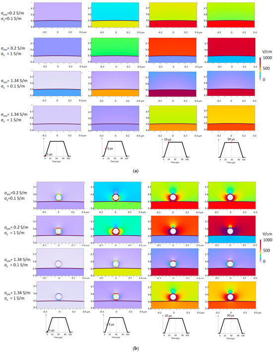
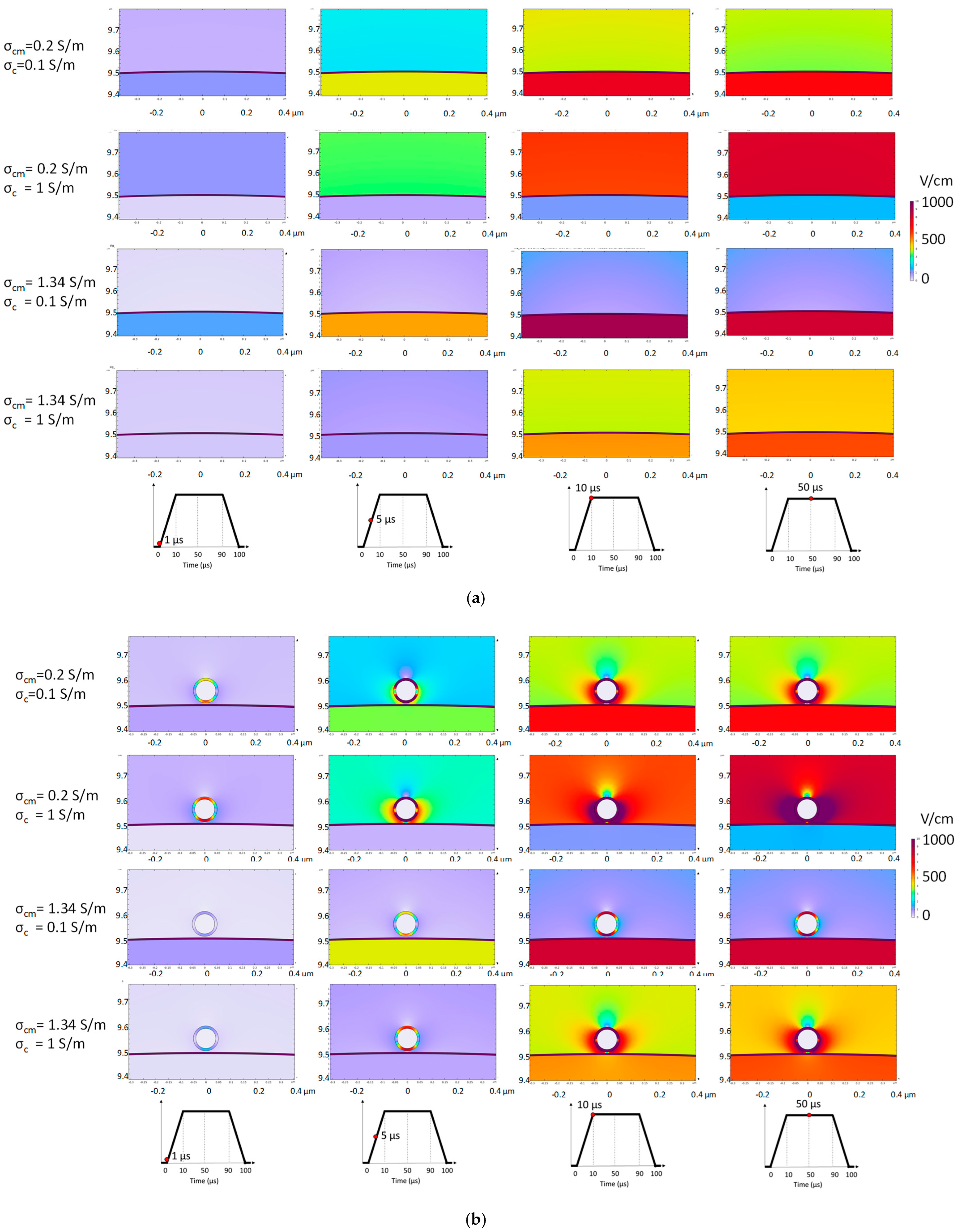
Color maps of electric field distribution (a) without and (b) with a magnetic nanoparticle at the 4 considered time instants (1, 5, 10 and 50 µs) on the pulse diagram, for an applied nominal electric field of 1000 V/cm.
Each column in the panel furnishes the field strength at a fixed time instant during the time-varying applied input, the 10 V amplitude trapezoidal-shaped voltage pulse that ideally generates a uniform electric field of 1000 V/cm in the space between the 100 µm distant parallel plate electrodes of the created capacitor, where the ROI is, if a homogeneous, linear and isotropic dielectric material is considered in this area. The simulation results also explore the perturbation effect locally created by the NP made of a magnetic nanocluster covered by a dielectric thin layer of silica (SiO2) that is expected to influence the field uniformity in the ROI.
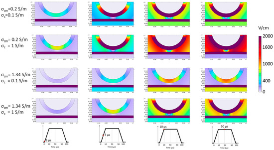
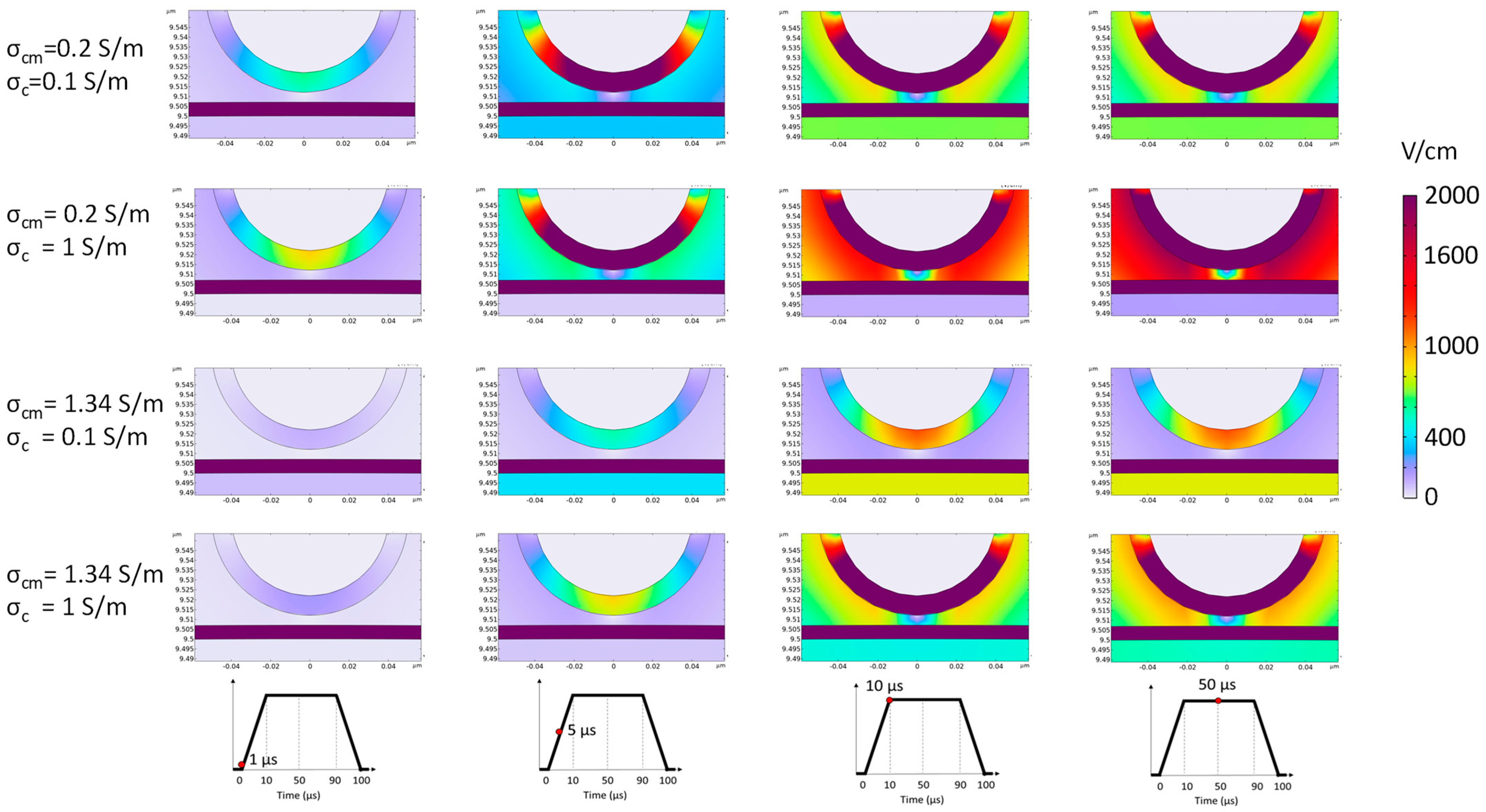
Figure 4 reports the color map related to the region close to the nanoparticle in four different time instants: the first three are located on the pulse rise time, whereas the last one is on the pulse plateau. Color maps are reported considering the four combinations of medium-cytosol conductivities listed in the materials and methods paragraph: two different conductivities for the surrounding medium and cytosol are considered. For all the considered cases, the ideal uniform 1000 V/cm of electric field strength is never obtained in the ROI up to 50 µs. The 1000 V/cm is reached in the whole model (shown in Figure 3) and, in some cases, close to the NP (see column 4 in Figure 4b). By comparing the rows of the panels (Figure 3 and Figure 4), it is evident that the conductivities of the surrounding mediums and cytosols affect the overall electric field intensity in the ROI and, in particular, in the region close to the NP. Moreover, the NP (Figure 4b) modifies the electric field distribution with respect to the field found in the media alone (Figure 4a). Importantly, Figure 5 shows a zoomed region of Figure 4b, highlighting the electric field distribution in the region between the NP and the cell membrane at four different time instants and for all four combinations of the electric conductivities of the cytosols and cell mediums. In particular, the electric field strength outside the cell is larger when the cell medium is less conductive, i.e., σcm = 0.2 Sm−1. Moreover, the electric field strength is larger when the cytosol conductivity is lower, i.e., σc = 0.2 Sm−1.
Figure 5.
Enlarged view of the color map showing the electric field distribution in the region between the nanoparticle and the cell membrane at the 4 considered time instants (1, 5, 10 and 50 µs) on the applied pulse diagram.
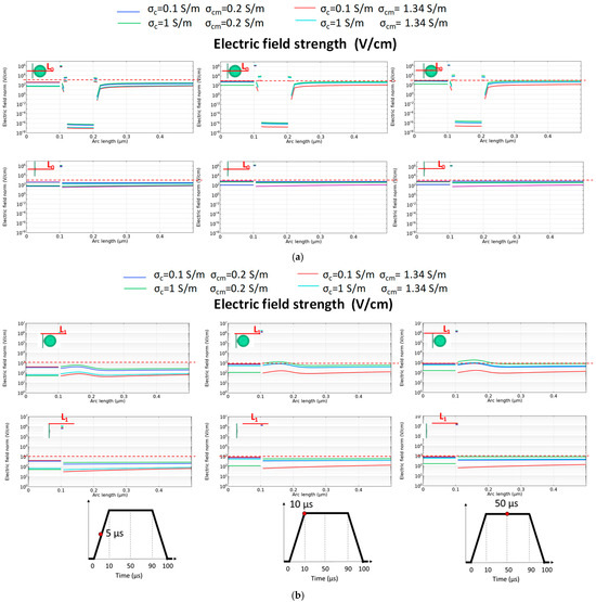
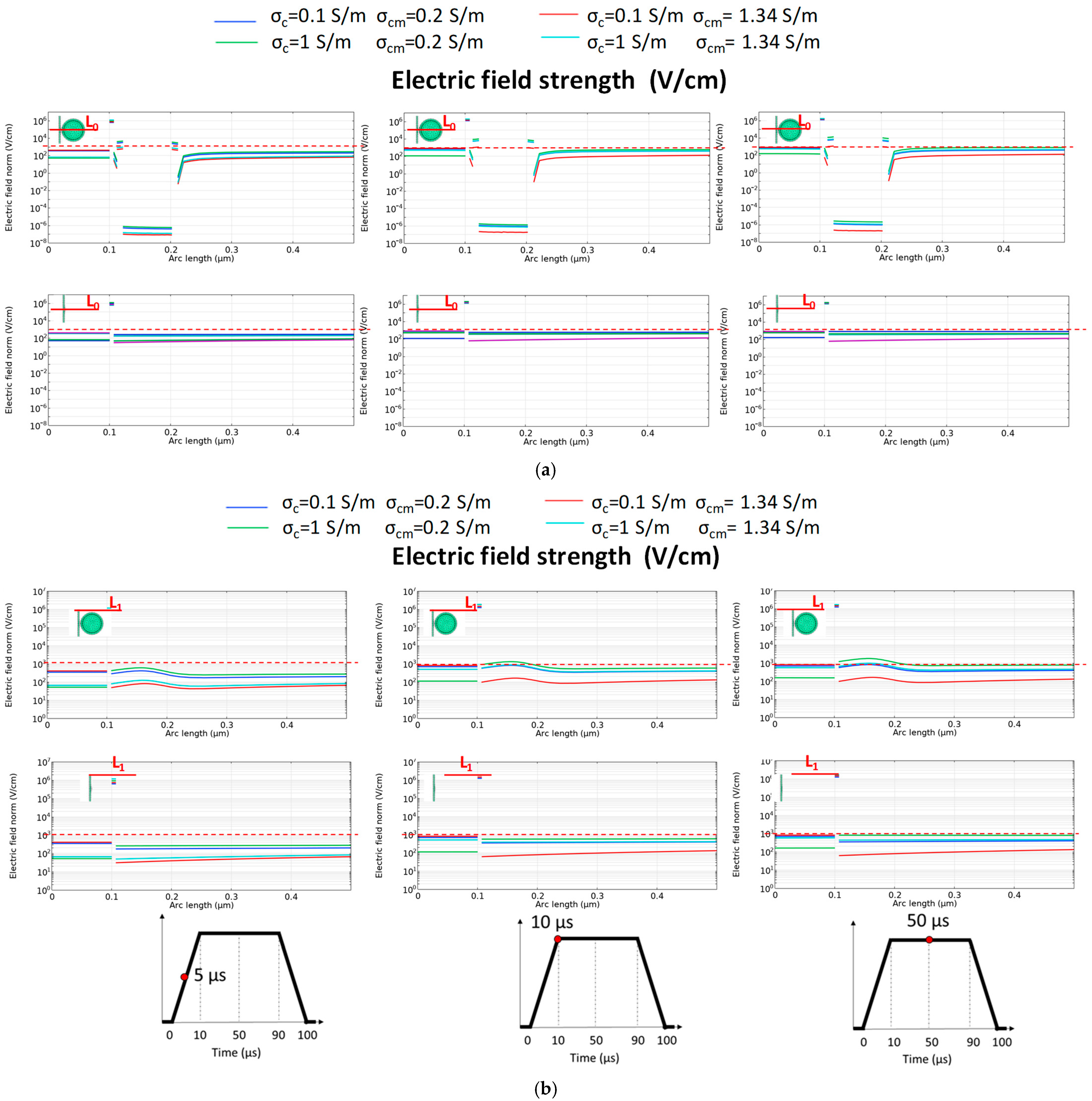
The electric field strength evaluated along the two red lines in Figure 2a is represented in Figure 6, considering the four analyzed cases for cytoplasm and medium conductivities.
Figure 6.
Electric field along red lines schematized in Figure 2a, (a) L0 and (b) L1 with (upper row) and without (lower row) magnetic nanoparticle corresponding to the four conductivity combinations (color lines in the upper legend) at the three time instants (5, 10 and 50 µs) on the pulse diagram. Dashed line mark the 103 V/cm level.
Figure 6a shows the case along the line L0 that cuts the NP in the middle, whereas Figure 6b analyzes the electric field strength on the line L1 that is tangential to the NP’s edge. It can be noted that the presence of the NP affects the electric field in the cytosol and in the region between the cell membrane and NP during pulse rise time with respect to the NO-nanoparticle conditions. The red dashed line marks the electric field strength at 1000 V/cm and during the pulse rise time, and the difference in the electric field strength with and without the NP can be evidenced at the 5 and 10 µs times. In particular, the electric field strength in the cell cytosol is lower considering the NP with respect to the case without the NP, as also remarked in Table 3.
Table 3.
Electric field strength at the four time instants marked in Figure 2c evaluated at the two points, P1 and P2, on line L0 marked in Figure 2b for the case with and without the silica-coated NP. Difference between Eint and Eext, i.e., Ed(i), percentage difference between the Ed(i) quantity with NP, Ed(NP) and without NP, Ed(NoNP).
Considering line L1 (Figure 6b) that samples the electric field on a vertical line just outside the NP, it can be noted that the presence of the NP modifies the distribution of the electric field. The horizontal dashed red line marks the 1000 V/cm level and it can be noted that the electric field in the NP ROI can be higher when the NP is considered.
Table 3 reports the electric field strength evaluated along line L0 in cytosol and medium at the membrane boundary at the two points, P1 and P2, marked in Figure 2b for the four time instants marked in Figure 2c. In particular, the electric field strength was evaluated in cytosol, Eint, i.e., the region internal to the cell, and in medium, Eext, i.e., the region external to the cell. Moreover, the difference between Eint and Eext, Ed(i) = Eext − Eint, with i = NP(nanoparticle) or NoNP(No-nanoparticle), is evaluated and it is positive or negative depending on the material conductivity. It is positive when the cytosol conductivity, σc, is larger than the medium conductivity, σcm, and negative in the inverse situation. It can be noted that the percentage variation with respect to the case without NP is constant for all the time instants analyzed when the cytosol conductivity is low, σc = 0.1 (S/m), and it is larger when the cytosol conductivity is 1 S/m. When the cytosol conductivity is σc = 1 (S/m), the entity of the percentage variation depends on the medium conductivity and it is larger for the time instant in the plateau (i.e., at 50 µs). In particular, the electric field strength is reduced by the presence of the NP if the evaluation points are located on the line L0. Nevertheless, considering the line L1, the electric field strength when the NP is close to the cell membrane is larger with respect to the case without the NP (data in Table 3). In fact, in the presence of the NP, the electric field in the medium is larger than the one in the absence of the NP. Nevertheless, the electric field difference Ed(i) between cytosol, Eint, and medium, Eext, is inferior to the one obtained without the NP, except in the case for which cytosol conductivity is higher than medium conductivity, i.e., σc = 1 (S/m) and σcm = 0.2 (S/m). In the case in which cytosol and medium conductivities are 1 and 1.34, the percentage difference between Ed(i) values is negative in the pulse plateau and positive in the pulse rise time. This means that in pulse rise time, Ed(i) in the presence of NP is larger than that without NP and at the plateau, it has a contrary behavior.
Considering the data in Table 4 refer to points P1 and P2 on the line L1, it can be noted that the electric field in the medium is larger than the one obtained in the ROI without the NP in all examined cases. The Ed(i) quantities have a different behavior than the one that occurs along Line L0 and the difference is larger than that of the cases analyzed in Table 3. This is in accordance with the data in Figure 4. In particular, along L1, the resulting percentage difference in the electric field between medium, Eext, and cytosol, Eint, i.e., Ed(i), depends on the considered case. Moreover, it is, in general, larger than that in the previous case (Table 3). With the NP, it is positive and larger than in the case without NP when σc (S/m) > σcm (S/m). Considering the other cases for which σc (S/m) < σcm (S/m), Ed(i) is positive if σc = 1 and σcm = 1.34 S/m, whereas it is negative in the other two cases.
Table 4.
Electric field strength at the four time instants marked in Figure 2c evaluated at the two points, P1 and P2, on line L1 marked in Figure 2b for the case with and without the silica-coated NP. Difference between Eint and Eext, i.e., Ed(i), percentage difference between the Ed(i) quantity with NP, Ed(NP) and without NP, Ed(NoNP).
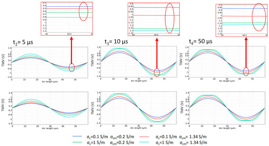
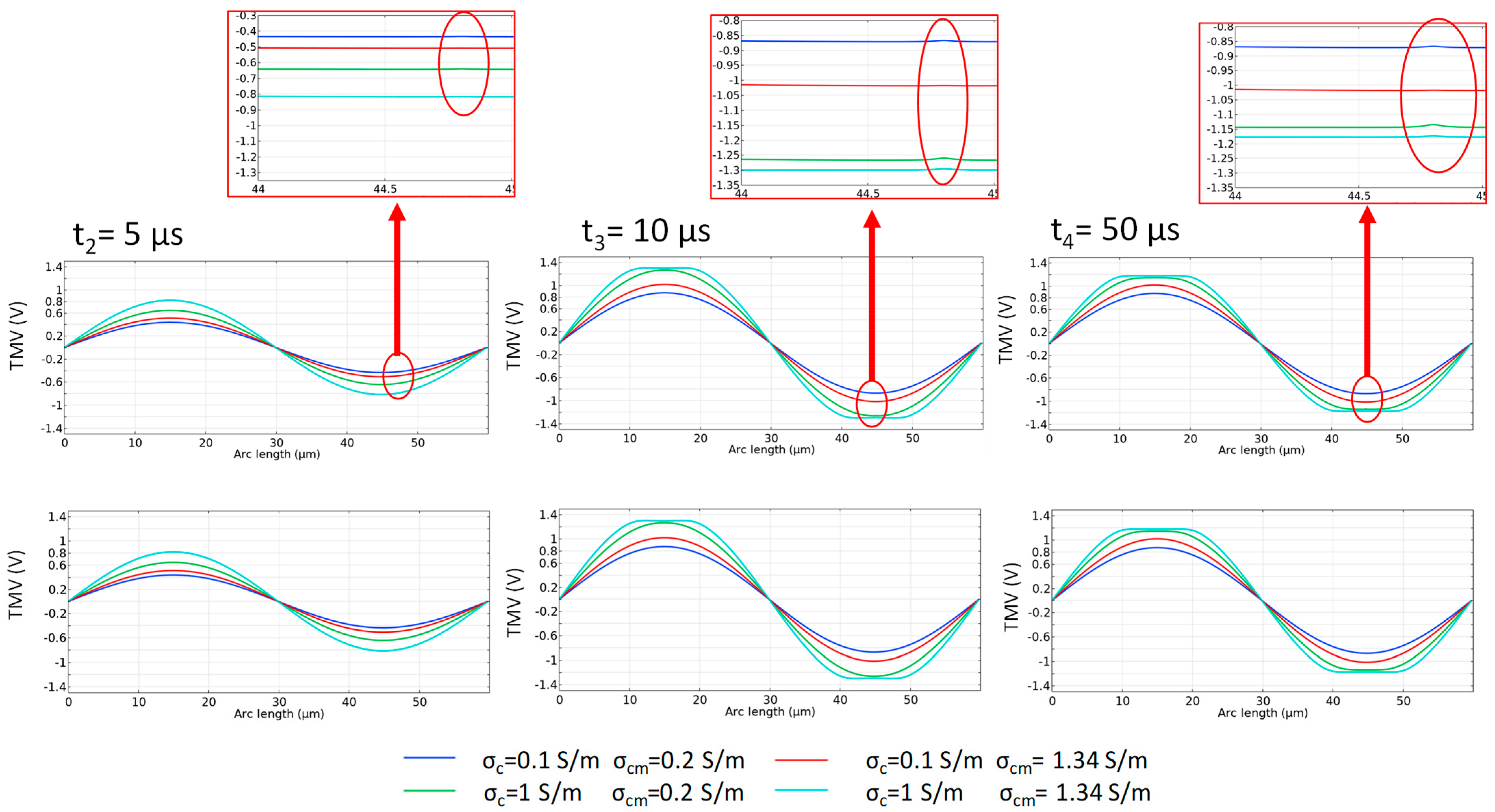
Figure 7 shows the TMV on the cell membrane region for all the four analyzed combinations of the cytosol–medium conductivities at three time instants (5 and 10 µs, located on the pulse rise time, and at 50 µs, located on the pulse plateau). It can be noted that nanoparticles positioned in the proximity of the cell membrane modulate the TMV during pulse rise time (evident at 5 and 10 µs). In particular, the TMV is lower in point P1 on the line L0 when the magnetic NP is close to the cell membrane. In Figure 7, the zoomed images evidence the effect of NP in the TMV that is locally distorted. Considering the data in Table 5, the electric potential evaluated at the points P1 and P2 on the line L0, marked in Figure 2b, for the four time instants marked in Figure 2c, is reported, whereas Table 6 reports the electric potential evaluated at the point P1 and P2 on the line L1. In these tables, the potential in cytosol and medium, Vint and Vext respectively, their difference Vd(i) = Vext − Vint (V), with i = NP(nanoparticle) or NoNP(No-nanoparticle), that corresponds to Vm in Equation (7) and the percentage difference between the Vd(i) quantity with NP, Vd(NP) and without NP, Vd(NoNP), are reported.
Figure 7.
TMV with (upper row) and without (lower row) magnetic nanoparticle at three time instants (5, 10 and 50 µs) on the pulse diagram.
Table 5.
TMV at the five time instants marked in Figure 2c evaluated at the two points, P1 and P2, on line L0 marked in Figure 2b for the case with and without the silica-coated NP. Difference between Vint and Vext, i.e., Vd(i), percentage difference between the Vd(i) quantity with NP, Vd(NP), and without NP, Vd(NoNP).
Table 6.
TMV at the four time instants marked in Figure 2c evaluated at the two points, P1 and P2, on line L1 marked in 2b for the case with and without the silica-coated NP. Fig. Difference between Vint and Vext, i.e., Vd(i), percentage difference between the Vd(i) quantity with NP, Vd(NP), and without NP, Vd(NoNP).
Table 5 reports the values of the TMV evaluated in cytosol and medium regions at the membrane boundary at the two points, P1 and P2, on the line L0 marked in Figure 2b for the four time instants marked in Figure 2c. In particular, the TMV is evaluated in cytosol, Vint, i.e., the region internal to the cell, and in medium, Vext, i.e., the region external to the cell. Moreover, the difference between Vext and Vint, TMV = Vd(i) = Vext − Vint (V), with i = NP(nanoparticle) or NoNP(No-nanoparticle), is evaluated and it is positive at every time point. The amplitude of the difference Vd(i) is different considering various combinations of material conductivities. The larger differences occur during the plateau when the cytosol conductivity is 1 S/m, where the conduction phenomena prevail, and it is minimum in the rise time when the medium conductivity is 1.34 S/m. Considering the data in Table 6, related to the two points, P1 and P2, on the line L1, the percentage difference of TMV between the case with and without the NP is lower with respect to the case in Table 5 and related to the point on the line L0. This way, the local increment of the electric field along line L1 has a detrimental effect on the TMV, considering only one NP.
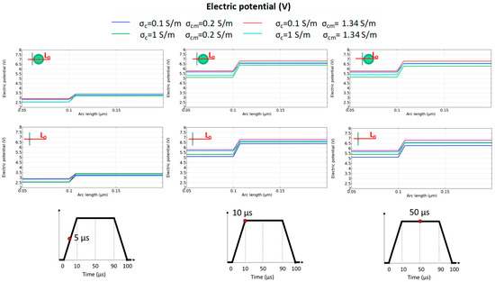
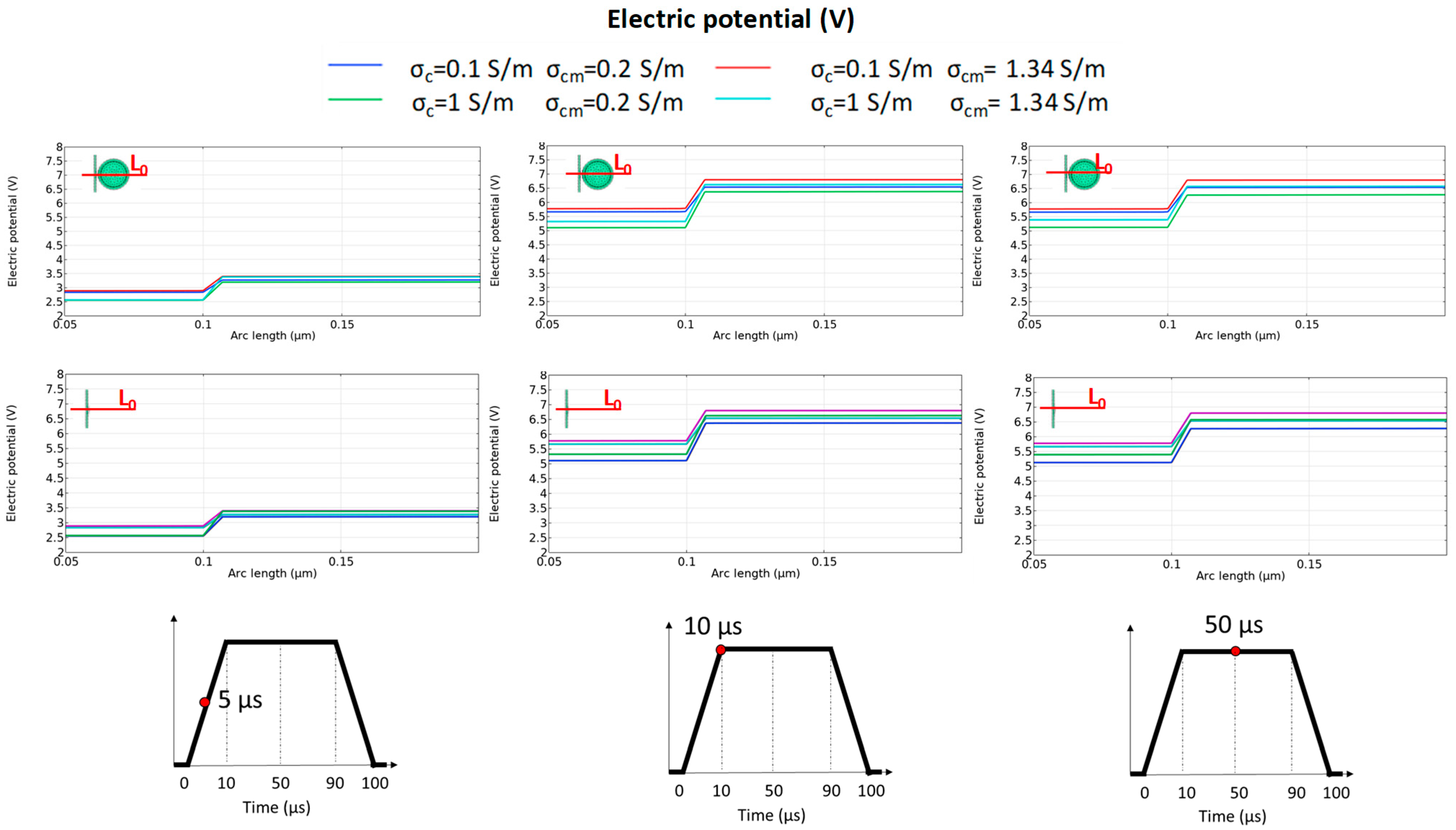
Figure 8 shows the electric potential on the line L0 (where the points P1 and P2 are located) evaluated at four time instants marked in Figure 2c. The electric potential increases during the pulse rise time. From Table 4 and Figure 8, it can be evidenced that on the points P1 and P2, the electric potential in the presence of the NP increases in the medium region and decreases in the cytosol regions. Then, the Vd(i) is larger where the NP is close to the cell membrane. At the end of the transient and in the plateau region, the electric potential in the cytosol is the same in both cases, with and without NP.
Figure 8.
Electric potential along the L0 red line in Figure 2a with (upper row) and without (lower row) magnetic nanoparticle at three time instants (5, 10 and 50 µs) on the pulse diagram.
Overall, the results based on numerical simulations indicate that a silica-coated magnetic nanoparticle adjacent to the cell membrane locally perturbs the electric field (Figure 4), and this perturbation depends on the medium surrounding the NP. Importantly, as shown in Figure 6, this perturbation can result in field reduction in some regions (Figure 6a related to line L0), as well as local enhancement in other regions (Figure 6b related to line L1), namely the nanoparticle’s edge.
The biologically relevant Figure 6 shows TMV modulation, where the magnetic silica-coated NP increases the local transmembrane voltage during the pulse rise time, but has little, if any, effect once the pulse reaches the plateau. The relative maximum increase in TMV is 0.8% and, in general, depends on the conductivity conditions. It is maximum on the line L0 where the external electric field is less influenced by the NP. The field-perturbation effect is therefore transient, local, geometry-dependent, and strongly influenced by the conductivity contrast between cytosol and extracellular medium.
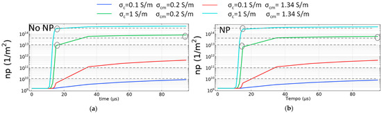
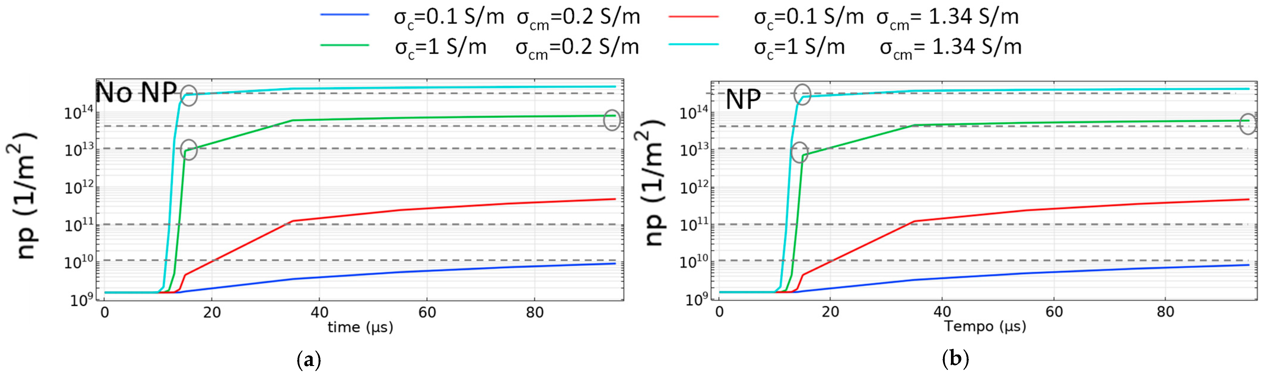
Figure 9 shows the pore-density dynamics in the four parameter combinations evaluating as a function of the time at the point P2 in Figure 2b on the cell membrane. It is evident that material conductivities affect the pore density and then the beginning of electroporation phenomena.
Figure 9.
Pore density at the point P2 in Figure 2b on the cell membrane as a function of the time (a) without the NP and (b) considering the NP at 50 µs.
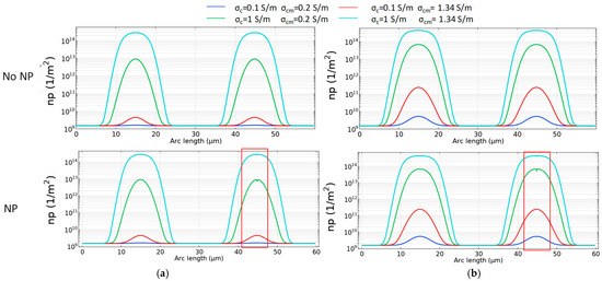
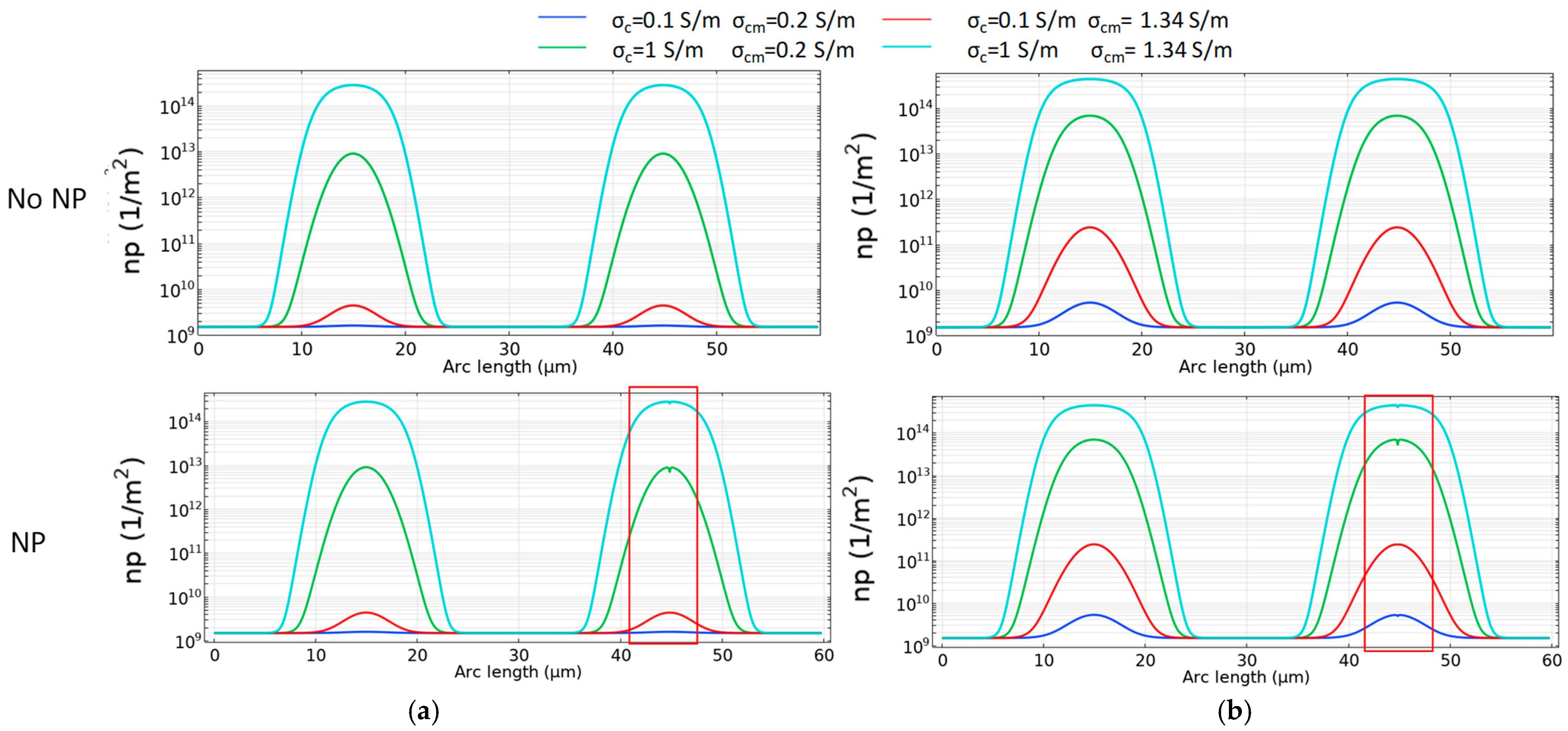
Finally, Figure 10 shows the pore density evaluated along the membrane domain at two time instants (10 and 50 µs). These time instants are more relevant since the pore density is increased with respect to the basal value of 1.5·109. The effect of the nanoparticle can be observed in the red rectangle and appears as a local reduction of pore density. The percentage difference between the pore density with and without the NP at three relevant time instants is reported in Table 7. The negative value shows the decrement of pore density in the presence of the nanoparticle in the proximity of the point P2. Moreover, the different material conductivities influence the pore density more when the conductivity gap between the conductivities is larger. Table 8 shows the percentage difference between the pore density with and without the NP in the plateau (at 50 µs), which is positive, in the points before the curve maximum that occurs in the position 44.8 µm in Figure 10. At these points, this percentage difference is positive; then, the magnetic NP increases the pore density at some points in the membrane. The percentage difference in position 30.5 µm, i.e., a point in the cell membrane at 90° with respect to NP position, is reported in order to show that there is a minimum in the percentage difference, that is few orders of magnitude with respect to the ones in positions between 40 and 50 µm (the curve is symmetric for the given geometry).
Figure 10.
Pore density along the cell domain for the cases without NP (top row) and with NP (bottom row) for the four combinations of material conductivities at the time instant times (a) 10 µs and (b) 50 µs corresponding to the rise time middle and plateau middle, considering the trapezoidal pulse diagram.
Table 7.
Pore-density Np at the point P2 in Figure 2b at three relevant time instants (5, 10 and 50 µs) for the case with and without the silica-coated NP. Fig. Percentage difference between the Np(i) quantity with NP, Np(NP), and without NP, Np(NoNP).
Table 8.
Pore density Np at some points along the cell membrane (at 30.5 µm and in the red area in Figure 8) at 50 µs for the case with and without the silica-coated NP. Fig. Percentage difference between the Np(i) quantity with NP, Np(NP), and without NP, Np(NoNP).
The presented results show the effect of one silica-coated magnetic nanocluster on the electric distribution in a region close to the cell membrane during electroporation pulse application. This study includes a transient simulation and conduction and displacement current were considered, while the magnetic component is also included, since the magnetic core has a not-unitary relative magnetic permeability, close to 1.86. Although magnetic permeability formally enters Maxwell’s equations through the A–V formulation, the relatively low permeability value of the iron oxide core (μr = 1.86), combined with the absence of external magnetic excitation and the transient low-frequency regime considered here, suggests that magnetic contributions to the observed electric field perturbation are expected to remain secondary compared with conductivity- and permittivity-driven effects. Consequently, we do not interpret the observed local field redistribution as evidence of a biologically relevant magnetoelectric coupling mechanism, but rather as a consequence of local electromagnetic heterogeneity introduced by the nanoparticle structure. A dedicated sensitivity analysis specifically varying μr would be required to fully isolate the contribution of magnetic permeability, but such analysis falls beyond the scope of the present study.
While our model can be considered informative, we recognize that our model does not represent the complex realities of a biological experiment, where nanoparticles do not remain perfectly stationary at a fixed 5 nm distance from the membrane, as they might undergo Brownian motion, electrophoretic drag induced by the external electric pulses, hydrodynamic flows and other perturbations. Furthermore, in vitro experiments rarely feature perfectly isolated single cells with uniform cytosol conductivity in a perfectly homogeneous medium, as well as isolated nanoparticles.
4. Conclusions
This numerical study shows that a silica-coated magnetic nanoparticle positioned in close proximity to the cell membrane can locally perturb the electric field distribution during an electroporation pulse. The perturbation is highly localized, depends on the nanoparticle–membrane geometry, and is strongly influenced by the conductivity contrast between the cytosol and the extracellular medium. Although local changes in transmembrane voltage are observed during the pulse rise time, their magnitude remains modest and they largely disappear once the pulse reaches the plateau. Importantly, the nanoparticle does not produce a uniform enhancement of electroporation-related parameters; depending on the location considered, it may increase or reduce the local electric field, and the pore-density analysis indicates a local decrease near the nanoparticle under several conductivity conditions. Therefore, the main outcome of the model is not a generalized enhancement of electroporation, but the identification of transient nanoscale field redistribution induced by a membrane-proximal silica-coated magnetic nanoparticle. These results should be interpreted as comparative trends within a 2D effective-medium model and require future 3D modeling and experimental validation before conclusions can be drawn on magnetic nanoparticle-assisted electroporation efficacy.
Author Contributions
Conceptualization, E.S. and P.L.; methodology, E.S., P.L., M.P., J.K.-T., S.K., M.F. and V.T.; formal analysis, E.S. and M.F.; investigation, E.S., P.L., S.K., M.M. and A.G.; data curation, E.S.; writing—original draft preparation, E.S. and J.K.-T.; writing—review and editing, S.K. and V.T.; supervision, V.T. All authors have read and agreed to the published version of the manuscript.
Funding
P.L. European Union’s Horizon Europe research and innovation program under the Marie Skłodowska Curie grant agreement No 101086142 (FLORIN project) and by the Italian National Recovery and Resilience Plan (NRRP) of NextGenerationEU, Mission 4, Component 2, Investment 1.1, Call for tender No. 1409 of 14.9.2022 of the Italian Ministry of University and Research (MUR), Project Title DEEPEST (Digging into rEversible and irreversible ElectroPoration: in vitro and in silico multiphysical analyses on cEll modelS for cancer Treatment) CUP B53D23002500006—Grant Assignment Decree No. 960 of 30/06/2023. J.K.-T. kindly acknowledges the ANR funding, project JOULMECT (grant ANR-23-CE18-0029-01). S.K. kindly acknowledges the Slovenian Research and Innovation Agency (ARIS) funding through the core funding No. P2-0089 and ARIS projects: J2-60047, J1-70022, L2-60141.
Institutional Review Board Statement
Not applicable.
Informed Consent Statement
Not applicable.
Data Availability Statement
The datasets presented in this article are not readily available because the data is contained within the article. Requests to access the datasets should be directed to the corresponding authors.
Conflicts of Interest
The authors declare no conflicts of interest.
Abbreviations
The following abbreviations are used in this manuscript:
| NP | Nanoparticle |
| NoNP | No Nanoparticle |
| TMV | Transmembrane Voltage |
References
- Zimmermann, U.; Pilwat, G.; Riemann, F. Dielectric Breakdown of Cell Membranes. Biophys. J. 1974, 14, 881–899. [Google Scholar] [CrossRef] [Scilit] [PubMed]
- Gehl, J. Electroporation: Theory and Methods, Perspectives for Drug Delivery, Gene Therapy and Research. Acta Physiol. Scand. 2003, 177, 437–447. [Google Scholar] [CrossRef] [Scilit] [PubMed]
- Faurie, C.; Golzio, M.; Phez, E.; Teissié, J.; Rols, M.-P. Electric Field-Induced Cell Membrane Permeabilization and Gene Transfer: Theory and Experiments. Eng. Life Sci. 2005, 5, 179–186. [Google Scholar] [CrossRef] [Scilit]
- Teissié, J.; Eynard, N.; Gabriel, B.; Rols, M.P. Electropermeabilization of Cell Membranes. Adv. Drug Deliv. Rev. 1999, 35, 3–19. [Google Scholar] [CrossRef] [Scilit] [PubMed]
- Mir, L.M. Therapeutic Perspectives of In Vivo Cell Electropermeabilization. Bioelectrochemistry 2001, 53, 1–10. [Google Scholar] [CrossRef] [Scilit] [PubMed]
- De Caro, A.; Bellard, E.; Kolosnjaj-Tabi, J.; Golzio, M.; Rols, M.-P. Gene Electrotransfer Efficiency in 2D and 3D Cancer Cell Models Using Different Electroporation Protocols: A Comparative Study. Pharmaceutics 2023, 15, 1004. [Google Scholar] [CrossRef] [Scilit] [PubMed]
- Mir, L.M. Bases and Rationale of the Electrochemotherapy. Eur. J. Cancer Suppl. 2006, 4, 38–44. [Google Scholar] [CrossRef] [Scilit]
- Dermol, J.; Miklavčič, D. Predicting Electroporation of Cells in an Inhomogeneous Electric Field Based on Mathematical Modeling and Experimental CHO-Cell Permeabilization to Propidium Iodide Determination. Bioelectrochemistry 2014, 100, 52–61. [Google Scholar] [CrossRef] [Scilit] [PubMed]
- Denzi, A.; Strigari, L.; Di Filippo, F.; Botti, C.; Di Filippo, S.; Perracchio, L.; Ronchetti, M.; Cadossi, R.; Liberti, M. Modeling the Positioning of Single Needle Electrodes for the Treatment of Breast Cancer in a Clinical Case. Biomed. Eng. Online 2015, 14, S1. [Google Scholar] [CrossRef] [Scilit] [PubMed]
- Campana, L.G.; Bullo, M.; Di Barba, P.; Dughiero, F.; Forzan, M.; Mognaschi, M.E.; Sgarbossa, P.; Tosi, A.L.; Bernardis, A.; Sieni, E. Effect of Tissue Inhomogeneity in Soft Tissue Sarcomas: From Real Cases to Numerical and Experimental Models. Technol. Cancer Res. Treat. 2018, 17, 153303381878969. [Google Scholar] [CrossRef] [Scilit] [PubMed]
- Kranjc, M.; Miklavčič, D. Electric Field Distribution and Electroporation Threshold. In Handbook of Electroporation; Miklavcic, D., Ed.; Springer International Publishing: Cham, Switzerland, 2016; pp. 1–17. [Google Scholar]
- Sel, D.; Cukjati, D.; Batiuskaite, D.; Slivnik, T.; Mir, L.M.; Miklavcic, D. Sequential Finite Element Model of Tissue Electropermeabilization. Biomed. Eng. IEEE Trans. 2005, 52, 816–827. [Google Scholar] [CrossRef] [Scilit] [PubMed]
- Ramirez, J.A.; Figueiredo, W.P.; Vale, J.F.C.; Metzker, I.D.; Santos, R.G.; Mattos, M.S.; Camargos, E.R.; Lowther, D.A. Investigation of the Electroporation Effect in a Single Cell. COMPEL Int. J. Comput. Math. Electr. Electron. Eng. 2013, 32, 1692–1706. [Google Scholar] [CrossRef] [Scilit]
- Corovic, S.; Lackovic, I.; Sustaric, P.; Sustar, T.; Rodic, T.; Miklavcic, D. Modeling of Electric Field Distribution in Tissues during Electroporation. Biomed. Eng. Online 2013, 12, 16. [Google Scholar] [CrossRef] [Scilit] [PubMed]
- Miklavcic, D.; Corovic, S.; Pucihar, G.; Pavselj, N. Importance of Tumour Coverage by Sufficiently High Local Electric Field for Effective Electrochemotherapy. EJC Suppl. 2006, 4, 45–51. [Google Scholar] [CrossRef] [Scilit]
- Poignard, C.; Silve, A.; Wegner, L. Different Approaches Used in Modeling of Cell Membrane Electroporation. In Handbook of Electroporation; Springer: Cham, Switzerland, 2016; pp. 1–24. [Google Scholar]
- Canatella, P.J.; Black, M.M.; Bonnichsen, D.M.; McKenna, C.; Prausnitz, M.R. Tissue Electroporation: Quantification and Analysis of Heterogeneous Transport in Multicellular Environments. Biophys. J. 2004, 86, 3260–3268. [Google Scholar] [CrossRef] [Scilit] [PubMed]
- Mescia, L.; Chiapperino, M.A.; Bia, P.; Lamacchia, C.M.; Gielis, J.; Caratelli, D. Design of Electroporation Process in Irregularly Shaped Multicellular Systems. Electronics 2019, 8, 37. [Google Scholar] [CrossRef] [Scilit]
- Murovec, T.; Sweeney, D.C.; Latouche, E.; Davalos, R.V.; Brosseau, C. Modeling of Transmembrane Potential in Realistic Multicellular Structures Before Electroporation. Biophys. J. 2016, 111, 2286–2295. [Google Scholar] [CrossRef] [Scilit] [PubMed]
- Akbarzadeh, A.; Samiei, M.; Davaran, S. Magnetic Nanoparticles: Preparation, Physical Properties, and Applications in Biomedicine. Nanoscale Res. Lett. 2012, 7, 144. [Google Scholar] [CrossRef] [Scilit] [PubMed]
- Goya, G.F.; Asín, L.; Ibarra, M.R. Cell Death Induced by AC Magnetic Fields and Magnetic Nanoparticles: Current State and Perspectives. Int. J. Hyperth. 2013, 29, 810–818. [Google Scholar] [CrossRef] [Scilit]
- Chiaramello, E.; Fiocchi, S.; Bonato, M.; Gallucci, S.; Benini, M.; Parazzini, M. Use of Nanoparticles as Nanoelectrodes in Contact-Less Cell Membrane Permeabilization by Time-Varying Magnetic Field: A Computational Study. Appl. Sci. 2021, 11, 11121. [Google Scholar] [CrossRef] [Scilit]
- Sato, A.; Tamura, Y.; Sato, N.; Yamashita, T.; Takada, T.; Sato, M.; Osai, Y.; Okura, M.; Ono, I.; Ito, A.; et al. Melanoma-Targeted Chemo-Thermo-Immuno (CTI)-Therapy Using N-Propionyl-4-S-Cysteaminylphenol-Magnetite Nanoparticles Elicits CTL Response via Heat Shock Protein-Peptide Complex Release. Cancer Sci. 2010, 101, 1939–1946. [Google Scholar] [CrossRef] [Scilit] [PubMed]
- Duguet, E.; Vasseur, S.; Mornet, S.; Devoisselle, J.-M. Magnetic Nanoparticles and Their Applications in Medicine. Nanomedicine 2006, 1, 157–168. [Google Scholar] [CrossRef] [Scilit] [PubMed]
- Chiaramello, E.; Fiocchi, S.; Bonato, M.; Gallucci, S.; Benini, M.; Parazzini, M. Cell Transmembrane Potential in Contactless Permeabilization by Time-Varying Magnetic Fields. Comput. Biol. Med. 2021, 135, 104587. [Google Scholar] [CrossRef] [Scilit] [PubMed]
- Hou, W.; Song, W.Q.; Zhang, R.X.; Lomova, M.V.; Sadovnikov, A.V.; Song, Y.J. Nanomedicine-Mediated Immunotherapy for Cancer Treatment. ACS Biomater. Sci. Eng. 2026, 12, 1968–1990. [Google Scholar] [CrossRef] [Scilit] [PubMed]
- DeNardo, S.J.; DeNardo, G.L.; Miers, L.A.; Natarajan, A.; Foreman, A.R.; Gruettner, C.; Adamson, G.N.; Ivkov, R. Development of Tumor Targeting Bioprobes (111In-Chimeric L6 Monoclonal Antibody Nanoparticles) for Alternating Magnetic Field Cancer Therapy. Clin. Cancer Res. 2005, 11, 7087s–7092s. [Google Scholar] [CrossRef] [Scilit] [PubMed]
- Dennis, C.L.; Ivkov, R. Physics of Heat Generation Using Magnetic Nanoparticles for Hyperthermia. Int. J. Hyperth. 2013, 29, 715–729. [Google Scholar] [CrossRef] [Scilit]
- Jordan, A.; Wust, P.; Fähling, H.; John, W.; Hinz, A.; Felix, R. Inductive Heating of Ferrimagnetic Particles and Magnetic Fluids: Physical Evaluation of Their Potential for Hyperthermia. Int. J. Hyperth. 2009, 25, 499–511. [Google Scholar] [CrossRef] [Scilit]
- Chomoucka, J.; Drbohlavova, J.; Huska, D.; Adam, V.; Kizek, R.; Hubalek, J. Magnetic Nanoparticles and Targeted Drug Delivering. Pharmacol. Res. 2010, 62, 144–149. [Google Scholar] [CrossRef] [Scilit] [PubMed]
- Hu, S.-H.; Liao, B.-J.; Chiang, C.-S.; Chen, P.-J.; Chen, I.-W.; Chen, S.-Y. Core-Shell Nanocapsules Stabilized by Single-Component Polymer and Nanoparticles for Magneto-Chemotherapy/Hyperthermia with Multiple Drugs. Adv. Mater. 2012, 24, 3627–3632. [Google Scholar] [CrossRef] [Scilit] [PubMed]
- Su, D.; Ma, R.; Salloum, M.; Zhu, L. Multi-Scale Study of Nanoparticle Transport and Deposition in Tissues during an Injection Process. Med. Biol. Eng. Comput. 2010, 48, 853–863. [Google Scholar] [CrossRef] [Scilit] [PubMed]
- Chicheł, A.; Skowronek, J.; Kubaszewska, M.; Kanikowski, M. Hyperthermia—Description of a Method and a Review of Clinical Applications. Rep. Pract. Oncol. Radiother. 2007, 12, 267–275. [Google Scholar] [CrossRef] [Scilit]
- Gneveckow, U.; Jordan, A.; Scholz, R.; Brüss, V.; Waldöfner, N.; Ricke, J.; Feussner, A.; Hildebrandt, B.; Rau, B.; Wust, P. Description and Characterization of the Novel Hyperthermia- and Thermoablation-System MFH 300F for Clinical Magnetic Fluid Hyperthermia. Med. Phys. 2004, 31, 1444–1451. [Google Scholar] [CrossRef] [Scilit] [PubMed]
- Lu, A.-H.; Salabas, E.L.; Schüth, F. Magnetic Nanoparticles: Synthesis, Protection, Functionalization, and Application. Angew. Chem. Int. Ed. 2007, 46, 1222–1244. [Google Scholar] [CrossRef] [Scilit] [PubMed]
- Scaffaro, R.; Botta, L.; Lo Re, G.; Bertani, R.; Milani, R.; Sassi, A. Surface Modification of Poly(Ethylene-Co-Acrylic Acid) with Amino-Functionalized Silica Nanoparticles. J. Mater. Chem. 2011, 21, 3849–3857. [Google Scholar] [CrossRef] [Scilit]
- Hong, R.Y.; Feng, B.; Chen, L.L.; Liu, G.H.; Li, H.Z.; Zheng, Y.; Wei, D.G. Synthesis, Characterization and MRI Application of Dextran-Coated Fe3O4 Magnetic Nanoparticles. Biochem. Eng. J. 2008, 42, 290–300. [Google Scholar] [CrossRef] [Scilit]
- Fan, C.; Gao, W.; Chen, Z.; Fan, H.; Li, M.; Deng, F.; Chen, Z. Tumor Selectivity of Stealth Multi-Functionalized Superparamagnetic Iron Oxide Nanoparticles. Int. J. Pharm. 2011, 404, 180–190. [Google Scholar] [CrossRef] [Scilit] [PubMed]
- Ito, A.; Shinkai, M.; Honda, H.; Kobayashi, T. Medical Application of Functionalized Magnetic Nanoparticles. J. Biosci. Bioeng. 2005, 100, 1–11. [Google Scholar] [CrossRef] [Scilit] [PubMed]
- Kim, Y.-G.; Park, J.-H.; Yoon, J. Guidance Scheme of Magnetic Nanoparticles with Artificial Potential Field. In Proceedings of the 2021 21st International Conference on Control, Automation and Systems (ICCAS), Jeju, Republic of Korea, 12–15 October 2021; pp. 2086–2088. [Google Scholar]
- Xu, Z.; Mousavi, T.; Liu, X.; Birjandi, A.A.; Thanou, M.; Fan, H.; Ainslie, M. Recent Advances in Numerical Simulation of Magnetically Guided Drug Delivery Systems and Applications. Adv. Drug Deliv. Rev. 2026, 229, 115745. [Google Scholar] [CrossRef] [Scilit] [PubMed]
- Kumar, A.; Jena, P.K.; Behera, S.; Lockey, R.F.; Mohapatra, S.; Mohapatra, S. Multifunctional Magnetic Nanoparticles for Targeted Delivery. Nanomed. Nanotechnol. Biol. Med. 2010, 6, 64–69. [Google Scholar] [CrossRef] [Scilit] [PubMed]
- Lekner, J. Electroporation in Cancer Therapy Without Insertion of Electrodes. Phys. Med. Biol. 2014, 59, 6031–6042. [Google Scholar] [CrossRef] [Scilit] [PubMed]
- Guo, F.; Gou, X.; Sun, J.; Hong, J.; Zhang, Y. Modeling Methods in Overlapping Electroporation Treatments: Pulse Number Effects on Tissue Conductivity and Ablation Area. Electrochim. Acta 2024, 503, 144883. [Google Scholar] [CrossRef] [Scilit]
- Krassowska, W.; Filev, P.D. Modeling Electroporation in a Single Cell. Biophys. J. 2007, 92, 404–417. [Google Scholar] [CrossRef] [Scilit] [PubMed]
- Guo, F.; Qian, K.; Zhang, L.; Deng, H.; Li, X.; Zhou, J.; Wang, J. Anisotropic Conductivity for Single-Cell Electroporation Simulation with Tangentially Dispersive Membrane. Electrochim. Acta 2021, 385, 138426. [Google Scholar] [CrossRef] [Scilit]
- Qiu, H.; Joshi, R.P.; Pradhan, A. Simulation of Nanoparticle Based Enhancement of Cellular Electroporation for Biomedical Applications. J. Appl. Phys. 2014, 116, 184701. [Google Scholar] [CrossRef] [Scilit]
- Zu, Y.; Huang, S.; Liao, W.-C.; Lu, Y.; Wang, S. Gold Nanoparticles Enhanced Electroporation for Mammalian Cell Transfection. J. Biomed. Nanotechnol. 2014, 10, 982–992. [Google Scholar] [CrossRef] [Scilit] [PubMed]
- Polajžer, T.; Kranjc, M.; Kralj, S.; Caf, M.; Romih, R.; Hudoklin, S.; Rocca, F.; Miklavčič, D. Limited Efficacy of Nanoparticle-Assisted Electroporation for Membrane Permeabilization and Gene Electrotransfer. Pharmaceutics 2025, 17, 964. [Google Scholar] [CrossRef] [Scilit] [PubMed]
- Polajžer, T.; Kranjc, M.; Kralj, S.; Caf, M.; Romih, R.; Hudoklin, S.; Novickij, V.; Miklavčič, D. Modulation of Contactless High Intensity Pulsed Electromagnetic Field Induced Electroporation and Gene Delivery Efficacy Using Various Nanoparticles. Bioelectricity 2026, 8, 67–77. [Google Scholar] [CrossRef] [Scilit] [PubMed]
- Kolosnjaj-Tabi, J.; Gibot, L.; Fourquaux, I.; Golzio, M.; Rols, M.-P. Electric Field-Responsive Nanoparticles and Electric Fields: Physical, Chemical, Biological Mechanisms and Therapeutic Prospects. Adv. Drug Deliv. Rev. 2019, 138, 56–67. [Google Scholar] [CrossRef] [Scilit] [PubMed]
- Nemec, S.; Kralj, S.; Wilhelm, C.; Abou-Hassan, A.; Rols, M.-P.; Kolosnjaj-Tabi, J. Comparison of Iron Oxide Nanoparticles in Photothermia and Magnetic Hyperthermia: Effects of Clustering and Silica Encapsulation on Nanoparticles’ Heating Yield. Appl. Sci. 2020, 10, 7322. [Google Scholar] [CrossRef] [Scilit]
- Guo, F.; Qian, K.; Li, X.; Deng, H. Simulation Study of Cell Transmembrane Potential and Electroporation Induced by Time-Varying Magnetic Fields. Innov. Food Sci. Emerg. Technol. 2022, 81, 103117. [Google Scholar] [CrossRef] [Scilit]
- Hu, Q.; Joshi, R.P.; Miklavcic, D. Calculations of Cell Transmembrane Voltage Induced by Time-Varying Magnetic Fields. IEEE Trans. Plasma Sci. 2020, 48, 1088–1095. [Google Scholar] [CrossRef] [Scilit]
- Voyer, D.; Silve, A.; Mir, L.M.; Scorretti, R.; Poignard, C. Dynamical Modeling of Tissue Electroporation. Bioelectrochemistry 2018, 119, 98–110. [Google Scholar] [CrossRef] [Scilit] [PubMed]
- Kavian, O.; Leguèbe, M.; Poignard, C.; Weynans, L. “Classical” Electropermeabilization Modeling at the Cell Scale. J. Math. Biol. 2014, 68, 235–265. [Google Scholar] [CrossRef] [Scilit] [PubMed]
- Sieni, E.; Nemec, S.; Lamberti, P.; Romeo, S.; Sgarbossa, P.; Forzan, M.; Golzio, M.; Rols, M.P.; Kolosnjaj-Tabi, J.; Kralj, S. Electric Field Distribution in Cell Aggregates in Presence of Nanostructures Under Electroporation Pulses. In Proceedings of the 2023 IEEE Nanotechnology Materials and Devices Conference (NMDC); IEEE: Paestum, Italy, 2023; pp. 174–179. [Google Scholar]
- Goldberg, E.; Suárez, C.; Alfonso, M.; Marchese, J.; Soba, A.; Marshall, G. Cell Membrane Electroporation Modeling: A Multiphysics Approach. Bioelectrochemistry 2018, 124, 28–39. [Google Scholar] [CrossRef] [Scilit] [PubMed]
- DeBruin, K.A.; Krassowska, W. Modeling Electroporation in a Single Cell. I. Effects of Field Strength and Rest Potential. Biophys. J. 1999, 77, 1213–1224. [Google Scholar] [CrossRef] [Scilit] [PubMed]
- Ivorra, A.; Villemejane, J.; Mir, L. Electrical Modeling of the Influence of Medium Conductivity on Electroporation. Phys. Chem. Chem. Phys. PCCP 2010, 12, 10055–10064. [Google Scholar] [CrossRef] [Scilit] [PubMed]
- Čorović, S.; Mir, L.M.; Miklavčič, D. In Vivo Muscle Electroporation Threshold Determination: Realistic Numerical Models and In Vivo Experiments. J. Membr. Biol. 2012, 245, 509–520. [Google Scholar] [CrossRef] [Scilit] [PubMed]
- Chiapperino, M.A.; Bia, P.; Lamacchia, C.M.; Mescia, L. Electroporation Modelling of Irregular Nucleated Cells Including Pore Radius Dynamics. Electronics 2019, 8, 1477. [Google Scholar] [CrossRef] [Scilit]
- Ye, H.; Cotic, M.; Kang, E.E.; Fehlings, M.G.; Carlen, P.L. Transmembrane Potential Induced on the Internal Organelle by a Time-Varying Magnetic Field: A Model Study. J. Neuroeng. Rehabil. 2010, 7, 12. [Google Scholar] [CrossRef] [Scilit] [PubMed]
- Liang, W.; Yang, X.; Wang, J.; Wang, Y.; Yang, W.; Liu, L. Determination of Dielectric Properties of Cells Using AC Electrokinetic-Based Microfluidic Platform: A Review of Recent Advances. Micromachines 2020, 11, 513. [Google Scholar] [CrossRef] [Scilit] [PubMed]
- Zudans, I.; Agarwal, A.; Orwar, O.; Weber, S.G. Numerical Calculations of Single-Cell Electroporation with an Electrolyte-Filled Capillary. Biophys. J. 2007, 92, 3696–3705. [Google Scholar] [CrossRef] [Scilit] [PubMed]
- Lamberti, P.; Tucci, V.; Romeo, S.; Sannino, A.; Scarfì, M.R.; Zeni, O. nsPEF-Induced Effects on Cell Membranes: Use of Electrophysical Model to Optimize Experimental Design. IEEE Trans. Dielectr. Electr. Insul. 2013, 20, 1231–1238. [Google Scholar] [CrossRef] [Scilit]
- Pavlin, M.; Kandušer, M.; Reberšek, M.; Pucihar, G.; Hart, F.X.; Magjarevićcacute, R.; Miklavčič, D. Effect of Cell Electroporation on the Conductivity of a Cell Suspension. Biophys. J. 2005, 88, 4378–4390. [Google Scholar] [CrossRef] [Scilit] [PubMed]
- Pucihar, G.; Kotnik, T.; Kandušer, M.; Miklavčič, D. The Influence of Medium Conductivity on Electropermeabilization and Survival of Cells In Vitro. Bioelectrochemistry 2001, 54, 107–115. [Google Scholar] [CrossRef] [Scilit] [PubMed]
- Ferry, D.K.; Rode, D.L. Physical and Electrical Properties of Silica. Appl. Phys. Rev. 2025, 12, 011304. [Google Scholar] [CrossRef] [Scilit]
- Properties: Silica—Silicon Dioxide (SiO2). Available online: https://www.azom.com/properties.aspx?ArticleID=1114 (accessed on 4 October 2025).
- Gauthier, M.M. (Ed.) Engineered Materials Handbook Desk Edition; ASM International: Almere, The Netherlands, 1995. [Google Scholar]
- Bertacchini, C. Cliniporator: Medical Electroporation of Tumors. In Handbook of Electroporation; Miklavcic, D., Ed.; Springer International Publishing: Cham, Switzerland, 2017; pp. 1–36. [Google Scholar]
- Bertacchini, C.; Margotti, P.M.; Bergamini, E.; Lodi, A.; Ronchetti, M.; Cadossi, R. Design of an Irreversible Electroporation System for Clinical Use. Technol. Cancer Res. Treat. 2007, 6, 313–320. [Google Scholar] [CrossRef] [Scilit] [PubMed]
- IGEA. Available online: http://www.igeamedical.com/ (accessed on 15 April 2014).
- Binns, K.J.; Lawrenson, P.J.; Trowbridge, C.W. The Analytical and Numerical Solution of Electric and Magnetic Fields; Wiley: Chichester, UK, 1992. [Google Scholar]
- Meunier, G. The Finite Element Method for Electromagnetic Modeling; ISTE: London, UK; Wiley: Hoboken, NJ, USA, 2008. [Google Scholar]
- COMSOL. Available online: https://www.comsol.com/ (accessed on 5 July 2026).
- Glaser, R.W.; Leikin, S.L.; Chernomordik, L.V.; Pastushenko, V.F.; Sokirko, A.I. Reversible Electrical Breakdown of Lipid Bilayers: Formation and Evolution of Pores. Biochim. et Biophys. Acta (BBA) Biomembr. 1988, 940, 275–287. [Google Scholar] [CrossRef] [Scilit] [PubMed]
- Gowrishankar, T.R.; Weaver, J.C. An Approach to Electrical Modeling of Single and Multiple Cells. Proc. Natl. Acad. Sci. USA 2003, 100, 3203–3208. [Google Scholar] [CrossRef] [Scilit] [PubMed]
- Li, J.; Lin, H. The Current-Voltage Relation for Electropores with Conductivity Gradients. Biomicrofluidics 2010, 4, 013206. [Google Scholar] [CrossRef] [Scilit] [PubMed]
- Shamoon, D.; Dermol-Černe, J.; Rems, L.; Reberšek, M.; Kotnik, T.; Lasquellec, S.; Brosseau, C.; Miklavčič, D. Assessing the Electro-Deformation and Electro-Poration of Biological Cells Using a Three-Dimensional Finite Element Model. Appl. Phys. Lett. 2019, 114, 063701. [Google Scholar] [CrossRef] [Scilit]
- Milestone, W.; Baker, C.; Garner, A.L.; Joshi, R.P. Electroporation from Mitochondria to Cell Clusters: Model Development Toward Analyzing Electrically Driven Bioeffects over a Large Spatial Range. J. Appl. Phys. 2023, 133, 244701. [Google Scholar] [CrossRef] [Scilit]
- Tadic, M.; Kralj, S.; Jagodic, M.; Hanzel, D.; Makovec, D. Magnetic Properties of Novel Superparamagnetic Iron Oxide Nanoclusters and Their Peculiarity Under Annealing Treatment. Appl. Surf. Sci. 2014, 322, 255–264. [Google Scholar] [CrossRef] [Scilit]
- Modestino, M.; Galluzzi, A.; Sarno, M.; Polichetti, M. Study of the Coercivity Field in a Sample of NiFe2O4-OA Nanoparticles at Different Temperatures: Comparing the Different Processes to Evaluate TB by DC Measurements. In Proceedings of the 2023 IEEE Nanotechnology Materials and Devices Conference (NMDC), Paestum, Italy, 22–25 October 2023; pp. 259–263. [Google Scholar]

Disclaimer/Publisher’s Note: The statements, opinions and data contained in all publications are solely those of the individual author(s) and contributor(s) and not of MDPI and/or the editor(s). MDPI and/or the editor(s) disclaim responsibility for any injury to people or property resulting from any ideas, methods, instructions or products referred to in the content. |
© 2026 by the authors. Licensee MDPI, Basel, Switzerland. This article is an open access article distributed under the terms and conditions of the Creative Commons Attribution (CC BY) license.