


Abstract
Performance degradation caused by temporal-difference signal fluctuations and the inflexibility of fixed proximal constraints remains a key challenge in policy optimization algorithms. To address these issues, this article develops a Coherence-Adaptive Proximal Optimization (CAPO) method. We first derive a temporal-coherence-aware advantage estimation mechanism by measuring the directional consistency of temporal-difference residuals within a local time window. Based on this mechanism, short-horizon and long-horizon advantage estimates are adaptively integrated to provide a more stable and temporally reliable policy improvement signal. CAPO is then instantiated within the PPO framework by incorporating the temporal coherence mechanism into both advantage construction and proximal policy updates. The proposed method preserves the stable optimization structure of PPO while adaptively adjusting the clipping range according to sample-wise temporal coherence. In this way, CAPO allows more sufficient policy improvement when the learning signal is temporally consistent and imposes more conservative updates when the signal is unstable. Experiments on six representative OpenAI Gym control tasks show that CAPO achieves better or comparable performance than standard PPO in most benchmark environments, with statistically reliable improvements in three tasks and comparable final performance in two tasks. Meanwhile, the results also show that CAPO does not uniformly outperform PPO in all environments, indicating that its advantage is task-dependent. Overall, CAPO improves training stability and convergence behavior in several representative tasks, especially when local temporal feedback provides reliable policy-improvement information.
1. Introduction
In deep reinforcement learning (DRL), the improvement of policy performance fundamentally relies on the reliable construction of policy update signals [1]. For policy-gradient-based reinforcement learning algorithms, an agent typically estimates the advantage function from sampled trajectories and uses this signal to guide the policy toward actions that yield higher long-term returns. Therefore, advantage estimation not only determines the direction of policy-gradient updates, but also directly affects the update magnitude, training stability, and final control performance. This issue becomes particularly critical in continuous-control and high-dimensional decision-making tasks, where environmental feedback often exhibits strong temporal correlations and local fluctuations. Value function approximation errors, reward noise, and delayed trajectory returns can be propagated into the advantage function through temporal-difference residuals, thereby destabilizing the policy update signal [2,3,4]. Accordingly, extracting more reliable advantage information from temporal feedback remains a central challenge for improving the stability and convergence efficiency of deep policy optimization algorithms.
A substantial body of research has been devoted to improving policy-gradient estimation and stabilizing policy updates. Sutton et al. established the theoretical foundation of policy-gradient methods, providing a principled framework for directly optimizing parameterized policies [5]. Building upon this foundation, Konda and Tsitsiklis introduced the actor–critic architecture, in which a value function estimator is incorporated to reduce the variance of policy-gradient estimates and improve the efficiency of policy learning [6]. To further constrain the instability induced by overly aggressive policy updates, Schulman et al. proposed trust region policy optimization (TRPO), which restricts the update magnitude by imposing a Kullback–Leibler (KL) divergence constraint between the old and new policies, thereby mitigating policy degradation caused by excessively large updates [7]. Subsequently, proximal policy optimization (PPO) replaced the computationally expensive second-order constrained optimization in TRPO with a clipped surrogate objective. Owing to its favorable balance between training stability and implementation simplicity, PPO has become one of the most widely adopted on-policy policy optimization algorithms [8]. In parallel, generalized advantage estimation (GAE) introduced a bias–variance trade-off parameter, , to provide a continuous interpolation between Monte Carlo returns and temporal-difference estimates, offering an effective advantage estimation tool for PPO and related policy optimization methods [9]. Subsequent empirical studies have further shown that the performance of PPO and TRPO can be strongly affected by implementation details and algorithmic design choices, indicating the importance of careful baseline configuration and reproducible experimental settings [10,11].
Despite the strong stability and general applicability demonstrated by the combination of PPO and GAE across a wide range of control tasks, both its advantage estimation scheme and proximal constraint mechanism still exhibit inherent limitations [11,12]. First, GAE typically relies on a fixed parameter to control the temporal scale of advantage estimation. Recent PPO variants have attempted to improve advantage estimation and value function utilization from different perspectives. For example, partial advantage estimation reduces the bias caused by truncated GAE in finite rollouts, advantage reuse mechanisms further exploit advantage information to improve policy update efficiency, and phasic policy gradient separates policy and value function optimization phases to improve value learning [13,14,15]. A larger enables the estimator to incorporate more long-horizon return information, but it also makes the advantage estimates more susceptible to reward fluctuations and value function approximation errors. In contrast, a smaller places greater emphasis on local temporal-difference (TD) residuals, which can reduce variance but may weaken long-term credit assignment. Since the temporal stability of feedback signals varies substantially across samples during training, a fixed may not simultaneously satisfy the estimation requirements of both stable trajectory segments and highly fluctuating ones.
Second, PPO usually adopts a uniform clipping coefficient, , to constrain the policy probability ratio for all samples, without explicitly differentiating the reliability of their update signals [16]. To overcome this limitation, several studies have investigated adaptive, ratio-guided, or more strictly proximal policy constraints. For instance, adaptive clipping methods adjust the clipping behavior according to sample characteristics, Truly PPO further strengthens the control of policy updates, and candidate-ratio-guided PPO modifies the update process by exploiting information from probability ratios [16,17,18]. When the signs of TD residuals remain consistent within a local temporal window, the corresponding advantage signal is often supported by a clear directional trend, in which case a fixed clipping boundary may unnecessarily restrict effective policy improvement. Conversely, when TD residuals change signs frequently within a local window, the current update signal may contain substantial noise; under such conditions, a uniform clipping constraint may be insufficient to suppress unreliable policy updates.
To address these limitations, recent studies have sought to further enhance policy learning from multiple perspectives, including exploration enhancement, value estimation improvement, policy constraint optimization, and empirical evaluation. Beyond general algorithmic development, reinforcement-learning-based control methods have been widely investigated in practical intelligent systems, including cooperative control of multiple unmanned vehicles, unmanned surface vehicle path planning, anti-disturbance control, cooperative autonomous driving, humanoid locomotion, and service robot task planning [19,20,21,22,23,24]. These studies demonstrate the broad applicability of reinforcement learning in dynamic control and decision-making scenarios, while also highlighting the importance of stable and reliable policy optimization mechanisms. Meanwhile, reliable empirical evaluation is also critical for deep reinforcement learning, since conclusions based only on mean performance over a limited number of random seeds may be statistically unreliable, and continuous-control benchmarks provide an important basis for comparing policy optimization methods across different control tasks [25,26]. Chen et al. and Wang et al. respectively introduced dynamically adjusted entropy and cognitive entropy mechanisms into ship collision-avoidance scenarios, enabling PPO-based methods to adaptively regulate exploration intensity and improve convergence behavior in complex decision-making tasks [27,28]. Duan et al. proposed distributional soft actor–critic, which learns the state–action return distribution to alleviate Q-value overestimation and thereby improves policy performance in continuous-control tasks [29]. Liu et al. further introduced a distributional value function into policy-gradient estimation, allowing the policy gradient to exploit distributional value information rather than relying solely on expected value estimates, which enhances exploration capability [30]. In addition, Cheng et al. improved the stability of policy improvement by introducing a relative-entropy constraint into the actor–critic framework, while Shang et al. extended relative-entropy regularization to continuous dynamic policy programming to improve both learning stability and sample efficiency in continuous action spaces [31,32].
It should be noted that the aforementioned studies mainly focus on enhancing exploration, improving value estimation accuracy, or constraining the magnitude of policy updates. However, within the standard PPO framework, the temporal scale of advantage estimation and the clipping boundary of policy updates are still typically governed by fixed hyperparameters, and these two components are not jointly adapted according to the reliability of local temporal feedback [14]. In other words, most existing methods implicitly assume that advantage signals at different time steps possess a comparable level of reliability, while overlooking the directional consistency exhibited by TD residuals within local temporal windows [18]. In fact, TD residuals not only reflect the estimation discrepancy between immediate rewards and the value function, but also encode implicit information about whether the return trend of the current trajectory segment is temporally stable. When the directions of TD residuals remain consistent across adjacent time steps, the corresponding policy improvement signal is supported by stronger temporal continuity. Conversely, when positive and negative TD residuals frequently cancel each other within a local window, the resulting advantage estimate may be substantially affected by noise, local perturbations, or value-estimation errors. Therefore, how to exploit the local directional consistency of TD residuals to construct a policy optimization mechanism that can simultaneously regulate advantage estimation and the policy clipping range remains an important problem worthy of further investigation [33].
Motivated by the above discussion, this paper proposes a coherence-adaptive proximal optimization algorithm (CAPO), which aims to improve the training stability and convergence efficiency of PPO through the coordinated design of advantage estimation and proximal policy constraints. Specifically, we first construct a temporal reliability measure based on the local directional consistency of TD residuals, which is used to evaluate whether the update signal of a given sample exhibits a stable trend within a local temporal window. Then, guided by the resulting temporal coherence coefficient, CAPO adaptively integrates short-horizon and long-horizon advantage estimates, enabling the advantage construction process to dynamically balance low variance and low bias according to the reliability of temporal feedback. Furthermore, the same temporal coherence coefficient is incorporated into the clipped surrogate objective of PPO to construct a sample-wise dynamic clipping boundary. In this way, policy updates are allowed to explore a broader optimization region for samples with high temporal coherence, while being subject to stricter proximal constraints for samples with low temporal coherence.
The main contributions of this work are summarized as follows.
- (1)
- We propose a temporal coherence measurement mechanism based on the local directional consistency of TD residuals. By characterizing the stability of update signals within a local temporal window, this mechanism provides a unified sample-wise reliability criterion for both advantage estimation and policy updates. It enables the algorithm to distinguish stable trajectory segments from highly fluctuating ones, thereby reducing the dependence of policy optimization on a fixed form of temporal feedback modeling.
- (2)
- We develop a temporal-coherence-aware advantage construction method that adaptively integrates short-horizon and long-horizon advantage estimates. The resulting advantage signal combines the merits of low variance and low bias. Compared with conventional advantage estimation based on a fixed GAE parameter, the proposed method can dynamically adjust the temporal scale of advantage estimation according to the reliability of local temporal feedback, thereby improving the stability of policy update signals.
- (3)
- We propose a coherence-adaptive proximal optimization algorithm, termed CAPO. While preserving the stable optimization framework of PPO, CAPO embeds the temporal coherence coefficient into the clipped surrogate objective to form a sample-wise dynamic clipping mechanism. This design allows policy updates to automatically balance sufficient policy improvement and conservative proximal constraints according to signal reliability. Experimental results on multiple representative control tasks demonstrate that the proposed method improves training stability and achieves competitive or improved performance in several representative environments.
The remainder of this paper is organized as follows. Section 2 introduces the preliminaries of reinforcement learning, PPO, and advantage estimation. Section 3 presents the proposed temporal-coherence-aware advantage estimation and adaptive proximal update mechanisms, and further instantiates them within the PPO framework as CAPO. Section 4 describes the experimental design and reports the simulation results. Finally, Section 5 concludes this study and discusses potential directions for future work.
2. Preliminaries
This section introduces the theoretical foundations required for the proposed method. We first formulate the reinforcement learning problem as a Markov decision process (MDP). Then, we review the basic objective of proximal policy optimization (PPO). Finally, we describe the construction of generalized advantage estimation (GAE) and temporal-difference (TD) residuals, and analyze how the temporal scale of advantage estimation affects policy updates. These preliminaries provide the theoretical basis for the temporal-coherence-aware advantage estimation and adaptive proximal update mechanisms proposed in Section 3.
2.1. Markov Decision Process
Reinforcement learning is essentially a sequential decision-making problem that arises from the interaction between an agent and its environment. Such a problem is commonly formulated as a Markov decision process (MDP) [34]. A standard MDP can be defined as a five-tuple:
where denotes the state space, denotes the action space, and represents the state transition probability function, which specifies the conditional probability of transitioning to the next state after executing action a in state s. The function denotes the immediate reward function, which characterizes the feedback obtained from the current state–action pair, and is the discount factor used to balance immediate rewards and long-term returns.
At time step t, the agent selects an action from the current state according to a policy . The environment then returns the next state and the immediate reward . Through continuous interaction, the agent generates a trajectory:
The goal of reinforcement learning is to learn an optimal policy that maximizes the expected discounted cumulative return, which can be formulated as:
where denotes the trajectory induced by policy , and denote the state and action at time step t, respectively, and represents the expectation over the trajectory distribution generated by the policy . For policy-gradient-based reinforcement learning algorithms, the policy parameters are iteratively updated by maximizing the objective function in Equation (3). The decision-making process of an MDP is illustrated in Figure 1.
Figure 1.
Illustration of the Markov decision process, where the agent interacts with the environment by selecting actions according to its policy and receiving states and rewards from the environment.
2.2. Proximal Policy Optimization
Proximal policy optimization (PPO) is a representative on-policy policy optimization algorithm that has been widely used in deep reinforcement learning [35]. Its core idea is to improve training stability by constraining the magnitude of policy changes when updating the policy using trajectories sampled from the current policy. Let denote the parameters of the old policy and denote the parameters of the current policy to be optimized. The importance sampling ratio between the new and old policies is defined as:
This ratio measures the change in the probability of selecting action under state when moving from the old policy to the current policy. Specifically, indicates that the current policy increases the probability of selecting the action, whereas indicates that the current policy decreases this probability.
Based on the importance sampling ratio, PPO constructs the following clipped surrogate objective:
where denotes the advantage estimate at time step t, is the clipping coefficient, and restricts the policy probability ratio to the interval . The clipped objective plays a key role in stabilizing policy optimization. When the probability ratio between the new and old policies remains within a reasonable range, the algorithm follows the standard policy-gradient update. However, when the policy update becomes excessively large, the clipping mechanism prevents the objective from increasing further, thereby suppressing unstable updates and reducing training oscillations.
It should be emphasized that, in PPO, both the direction and intensity of policy updates are mainly determined by the advantage estimate . When , the algorithm tends to increase the probability of selecting the corresponding action; when , it tends to decrease this probability. Therefore, the quality of advantage estimation directly affects the effectiveness of policy optimization in PPO [15]. If the advantage signal is corrupted by noise, value-estimation errors, or local reward fluctuations, PPO may still update the policy along an unreliable direction even though the clipping mechanism limits the magnitude of policy changes. Consequently, constructing a more stable and reliable advantage signal is crucial for further improving the performance of PPO.
2.3. Generalized Advantage Estimation and TD Residual
In the actor–critic framework, the advantage function is commonly used to measure how much better or worse a specific action is compared with the average behavior under the current state [36]. Let denote the state-value function parameterized by . The temporal-difference (TD) residual at time step t can be defined as:
where denotes the terminal indicator. When , the current state is terminal, and the value of the next state is no longer included. When , the TD residual incorporates both the immediate reward and the estimated value of the next state. Therefore, the TD residual reflects the discrepancy between the one-step feedback and the value function prediction, and it serves as a fundamental building block for advantage estimation.
To balance estimation bias and variance, generalized advantage estimation (GAE) constructs the advantage signal by exponentially accumulating multi-step TD residuals [37]. It is formulated as:
where is the bias–variance trade-off parameter. When is large, the advantage estimator incorporates more long-horizon return information, leading to lower bias but potentially higher variance. In contrast, when is small, the advantage estimate relies more heavily on short-horizon TD information, which reduces variance but may weaken long-term credit assignment.
It can therefore be observed that essentially controls the temporal scale of advantage estimation. A fixed implies that all samples use the same temporal scale to construct advantage signals. However, during practical training, the stability of TD residuals varies across different trajectory segments. For trajectory segments in which the directions of TD residuals are relatively consistent, long-horizon advantage estimation can more fully exploit continuous feedback information. Conversely, for trajectory segments where positive and negative TD residuals fluctuate frequently, long-horizon accumulation may amplify unstable signals, making short-horizon advantage estimation more robust.
Based on this observation, the following section constructs a temporal coherence coefficient from the local directional consistency of TD residuals, which is used to adaptively integrate short-horizon and long-horizon advantages. Furthermore, this coefficient is introduced into the clipped objective of PPO to dynamically adjust the sample-wise proximal update range. In other words, the proposed method does not alter the fundamental optimization framework of PPO. Instead, it introduces a temporal-coherence-aware mechanism into two key components, namely advantage estimation and clipping constraints, thereby improving the reliability of policy update signals and the stability of the training process.
3. Methodology
This section presents the proposed coherence-adaptive proximal optimization method in detail. To address the limitations of standard PPO, where the temporal scale of advantage estimation is fixed and the proximal clipping boundary lacks sample-wise adaptability, we first construct a temporal coherence measurement mechanism based on the local directional consistency of TD residuals. Based on this mechanism, a temporal-coherence-aware advantage construction method is then developed by adaptively integrating short-horizon and long-horizon advantages, thereby producing a more reliable policy update signal. Finally, the constructed temporal coherence coefficient is further embedded into the clipped surrogate objective of PPO, leading to the proposed coherence-adaptive proximal optimization algorithm, termed CAPO.
3.1. Temporal Coherence Measurement
In standard PPO, policy updates typically rely on advantage estimates constructed by GAE [38]. However, the temporal scale in GAE is mainly controlled by a fixed parameter , making it difficult to adaptively adjust advantage estimation according to the stability of feedback signals in different trajectory segments. When the directions of TD residuals within a local temporal window are relatively consistent, the update signal in the corresponding trajectory segment exhibits stronger temporal continuity, and it is therefore appropriate to incorporate return information over a longer horizon. In contrast, when TD residuals frequently change signs within a local window, the update signal may be affected by reward noise, value-estimation errors, or local perturbations. In such cases, excessive long-horizon accumulation may amplify unreliable signals.
To characterize the above temporal feedback property, we first define the one-step TD residual based on the value function associated with the old policy:
where denotes the immediate reward at time step t, denotes the value function corresponding to the old policy, is the discount factor, and is the terminal indicator. When , the current state is terminal, and the value of the next state is excluded from the TD residual computation.
Let H denote the predefined length of the local coherence window. For time step t, we compute the signed accumulation and the absolute accumulation of local TD residuals starting from t, respectively, as follows:
where denotes the effective window length after considering terminal states. If a terminal state is encountered within the window, subsequent time steps are excluded from the coherence computation for the current time step.
Based on the above two quantities, the temporal coherence coefficient is defined as:
where is a small positive constant introduced to avoid division by zero, and . The value of is sufficiently small and serves only as a numerical stabilizer; therefore, it does not substantially affect the calculation of the temporal coherence coefficient. As shown in Equation (11), essentially characterizes the directional consistency of TD residuals within a local temporal window. When the TD residuals in the window have nearly consistent directions, the magnitude of the signed accumulation approaches the absolute accumulation, namely , and thus approaches 1. Conversely, when positive and negative TD residuals frequently cancel each other, becomes significantly smaller than , and approaches 0.
It should be emphasized that does not directly measure the magnitude of rewards or returns. Instead, it describes whether the current policy update signal exhibits a consistent temporal trend within a local time range. Therefore, this coefficient provides a unified sample-wise reliability criterion for subsequent advantage estimation and policy clipping. By introducing local temporal coherence into the modeling of policy update signals, CAPO compares the signed accumulation strength and the overall fluctuation strength of TD residuals within a local window, thereby determining whether the current advantage signal is supported by a stable temporal trend. In this way, CAPO can distinguish stable feedback from fluctuating feedback at the sample level, providing a unified basis for the subsequent adjustment of the advantage estimation time scale and the adaptive design of the proximal clipping boundary.
3.2. Coherence-Adaptive Advantage Construction
After obtaining the temporal coherence coefficient, we further construct a coherence-adaptive advantage estimator. Standard GAE uses a single parameter to control the temporal scale of advantage estimation. However, a fixed is difficult to simultaneously adapt to both stable and fluctuating trajectory segments. To address this issue, we define short-horizon and long-horizon advantage estimates separately, and then adaptively integrate them using the temporal coherence coefficient.
Specifically, given a smaller parameter and a larger parameter , where , the short-horizon advantage estimate is defined as:
and the long-horizon advantage estimate is defined as:
where T denotes the ending time step index of the finite trajectory segment used for advantage estimation. In practical implementation, T corresponds to the last transition stored in the current rollout buffer for GAE computation. If a terminal state is encountered before the end of the segment, the accumulation is truncated at the terminal state through the terminal indicator. Therefore, T is different from the local coherence window length H and does not denote the total number of training time steps. In addition, relies more heavily on local TD information and thus has lower variance and stronger conservativeness, whereas incorporates more long-horizon return information and can provide more sufficient credit assignment. Nevertheless, when TD residuals fluctuate strongly, the long-horizon estimate may introduce higher variance.
Based on the above two advantage estimates, the CAPO advantage is constructed as:
As shown in Equation (14), the CAPO advantage is a convex combination of the short-horizon and long-horizon advantages. When approaches 1, the local TD residuals exhibit strong directional consistency, indicating that the current update signal is supported by a stable temporal trend. In this case, CAPO assigns a larger weight to the long-horizon advantage estimate to more fully exploit long-term return information. Conversely, when approaches 0, the local TD residuals show substantial directional conflicts, indicating that the current update signal has lower reliability. In this case, CAPO relies more on the short-horizon advantage estimate to reduce the interference of unstable signals in policy updates.
It should be noted that the proposed advantage construction does not empirically select among several fixed values. Instead, it uses local temporal coherence as an adaptive modulation factor for the temporal scale of advantage estimation. For samples with stable temporal feedback, CAPO increases the contribution of the long-horizon advantage, allowing the policy update to better exploit return information across multiple time steps. For samples with fluctuating temporal feedback, CAPO strengthens the influence of the short-horizon advantage to suppress the propagation of local noise and value-estimation errors during multi-step accumulation. As a result, the constructed advantage signal can dynamically balance low bias and low variance according to the feedback reliability of different trajectory segments, thereby providing a more stable optimization basis for subsequent policy updates.
To further improve training stability, the CAPO advantage is normalized within each training batch:
where and denote the mean and standard deviation of in the current batch, respectively. The normalization operation mitigates the influence of advantage-scale variations on the magnitude of policy-gradient updates across different training stages. In practical implementation, the normalized advantage can also be clipped to prevent extreme advantage values from causing excessively large gradient updates.
3.3. Coherence-Adaptive Proximal Policy Optimization
Based on the coherence-adaptive advantage estimator constructed in the previous subsection, we further embed the temporal coherence coefficient into the proximal policy update objective of PPO, leading to the proposed CAPO algorithm. It should be emphasized that the core of CAPO is not to alter the fundamental proximal optimization framework of PPO, but to use temporal coherence to jointly modulate advantage estimation and the clipping boundary. In this way, the policy update can adaptively adjust its update range according to the reliability of local temporal feedback.
Let denote the parameters of the old policy and denote the parameters of the current policy to be optimized. For the state–action pair at time step t, the importance sampling ratio is defined as:
In standard PPO, the clipping coefficient is usually treated as a global fixed hyperparameter. In contrast, CAPO constructs a sample-wise dynamic clipping boundary according to the temporal coherence coefficient:
where and denote the lower and upper bounds of the clipping range, respectively. Since , the dynamic clipping coefficient satisfies:
When is large, the advantage signal of the current sample is supported by stronger local temporal coherence. CAPO therefore applies a relatively relaxed proximal constraint, allowing the policy to make more sufficient use of reliable feedback for effective improvement. Conversely, when is small, the advantage signal may be affected by local noise, value-estimation errors, or short-term fluctuations. In this case, CAPO adopts a more conservative proximal constraint to reduce the interference of unreliable updates during policy iteration. Through this design, CAPO transforms the globally fixed clipping boundary in standard PPO into a temporal-coherence-driven sample-wise dynamic clipping mechanism, thereby improving the adaptability of policy updates to variations in local feedback quality.
Based on the CAPO advantage estimate and the dynamic clipping boundary, the actor objective of CAPO is formulated as:
where denotes the normalized CAPO advantage estimate, and is the sample-wise dynamic clipping coefficient. As shown in Equation (19), CAPO preserves the basic structure of the PPO clipped surrogate objective, while replacing the fixed advantage estimate and the fixed clipping boundary with a temporal-coherence-aware advantage estimate and a dynamic proximal constraint, respectively.
In practical optimization, to remain consistent with the standard actor–critic framework, we further incorporate the value function loss and the entropy regularization term. The overall optimization loss of CAPO is defined as:
where and denote the coefficients of the value function loss and entropy regularization, respectively, and denotes the policy entropy. The value function loss is used to constrain the estimation error of the critic and is written as:
where denotes the value learning target. In this work, the value target is constructed by combining the unnormalized CAPO advantage with the old value estimate:
Equation (22) can be further interpreted as a coherence-weighted adaptive return target. Since is constructed as a convex combination of the short-horizon and long-horizon advantage estimates, the corresponding value target can be equivalently written as:
Therefore, the critic is not trained with a completely independent Monte Carlo return target, but with a temporal-coherence-adaptive bootstrapped target that is consistent with the advantage signal used by the actor. This design helps align the actor update signal and the critic supervision signal under the same temporal reliability measure.
Nevertheless, this coupling may introduce a potential bias relative to an independent return target, especially when the temporal coherence coefficient is affected by value-estimation errors or noisy TD residuals. In this sense, Equation (23) reflects an adaptive bias–variance trade-off rather than an unbiased value target. When the local TD residuals are temporally consistent, the target gives more weight to the long-horizon return estimate; when the local signal fluctuates strongly, it shifts toward a shorter-horizon target to reduce variance. To reduce circular dependence during optimization, the target is computed from rollout data and the old value estimate, and is treated as a fixed regression target when updating the critic.
We have added this discussion to clarify the role and possible limitation of the value target in Equation (22). A more complete comparison between the proposed adaptive value target and independent return targets, such as Monte Carlo returns or fixed- bootstrapped targets, will be considered in future work to further evaluate the bias introduced by this coupling.
3.4. Mechanism Analysis
The core idea of CAPO can be summarized as using the local directional consistency of TD residuals to jointly regulate the temporal scale of advantage estimation and the constraint range of policy updates. Compared with standard PPO, CAPO exhibits two main mechanistic characteristics.
First, CAPO enables adaptive adjustment of the temporal scale in advantage estimation. Standard GAE relies on a fixed parameter, which means that all samples share the same temporal scale for advantage construction. In contrast, CAPO simultaneously constructs short-horizon and long-horizon advantage estimates and adaptively integrates them using the temporal coherence coefficient . When the local feedback signal is stable, CAPO increases the contribution of the long-horizon advantage, allowing the policy update to exploit more sufficient long-term return information. When the local feedback signal is unstable, CAPO increases the contribution of the short-horizon advantage, making the policy update more conservative. This mechanism alleviates the limited adaptability of fixed-parameter GAE under different sample conditions.
Second, CAPO enables sample-wise adaptation of the proximal clipping boundary. Standard PPO applies a uniform clipping coefficient to all samples, and thus cannot distinguish whether the update signal of each sample is reliable. In contrast, CAPO dynamically computes according to , such that samples with high temporal coherence are assigned a larger policy update region, whereas samples with low temporal coherence are subject to stricter proximal constraints. Therefore, CAPO does not simply enlarge or shrink the clipping range of PPO. Instead, it dynamically balances sufficient policy improvement and conservative updates according to the reliability of the local update signal.
Furthermore, when , CAPO degenerates into a conservative update form dominated by the short-horizon advantage and the minimum clipping range:
When , CAPO becomes a more sufficient update form dominated by the long-horizon advantage and the maximum clipping range:
Therefore, CAPO can be regarded as a continuous adaptive policy optimization mechanism that connects short-horizon conservative updates and long-horizon sufficient updates. This mechanism enables policy optimization to move beyond a single fixed temporal scale and a uniform clipping boundary, allowing the update behavior to be automatically adjusted according to local temporal feedback characteristics.
3.5. Algorithm Summary
The overall procedure of CAPO is summarized as follows. First, the agent interacts with the environment using the old policy and collects states, actions, rewards, terminal indicators, action log probabilities, and state-value estimates. Then, the TD residuals at each time step are computed using the old value function, and the temporal coherence coefficient is evaluated within a local temporal window. Next, the short-horizon and long-horizon advantages are constructed using and , respectively, and are adaptively fused by the temporal coherence coefficient to obtain the CAPO advantage. Finally, the CAPO advantage and the dynamic clipping boundary are embedded into the PPO clipped surrogate objective, and the actor and critic are jointly optimized.
The algorithmic comparison between PPO and CAPO is illustrated in Figure 2, and the pseudo-code of CAPO is presented in Algorithm 1.
| Algorithm 1 The proposed CAPO algorithm |
Input: Policy parameters , value parameters , discount factor , coherence window length H, GAE parameters and , clipping bounds and . Output: Optimized policy parameters .
|
Figure 2.
Workflow comparison between standard PPO and the proposed CAPO method, illustrating how CAPO introduces temporal-coherence measurement to adaptively regulate advantage estimation and the sample-wise clipping range.
Without modifying the fundamental actor–critic architecture of PPO, the proposed algorithm introduces a temporal-coherence-driven mechanism for jointly regulating advantage estimation and proximal policy constraints. Specifically, CAPO reconstructs the policy update signal through the adaptive fusion of short-horizon and long-horizon advantages, and dynamically adjusts the proximal clipping range according to local temporal coherence. In this manner, policy optimization is allowed to perform more sufficient improvement under reliable feedback, while maintaining conservative updates under fluctuating feedback. Meanwhile, this work further characterizes the update behavior of CAPO from multiple perspectives, including the temporal coherence level, dynamic clipping magnitude, policy distribution variation, and clipping ratio. These analyses provide a basis for subsequently evaluating the training stability and convergence characteristics of the proposed method in the experimental section.
Compared with standard PPO, CAPO introduces only a small amount of additional computation and does not change the fundamental actor–critic optimization framework. The extra computational cost mainly comes from three operations: calculating the local temporal coherence coefficient from TD residuals, constructing both short-horizon and long-horizon advantage estimates, and updating the sample-wise clipping coefficient. For a rollout segment with length N and a local coherence window of length H, the computation of temporal coherence has a complexity of in a direct implementation. Since H is a small fixed hyperparameter in this study, this additional cost is approximately linear with respect to the rollout length. The construction of the two GAE-style advantage estimates and the dynamic clipping coefficients also scales linearly with the number of sampled transitions.
It should be noted that CAPO does not introduce additional actor networks, critic networks, target networks, or extra environment interactions. The dominant computational cost of both PPO and CAPO still comes from neural network forward propagation, backpropagation, and multiple policy optimization epochs over the collected rollout data. Therefore, the overall computational complexity of CAPO remains close to that of standard PPO, with only lightweight sample-wise calculations added before the policy update. In practical implementation, these operations can be efficiently vectorized and do not substantially increase the training burden. This indicates that CAPO improves the adaptability of advantage estimation and proximal clipping while largely preserving the computational efficiency and implementation simplicity of PPO.
4. Experimental Results and Analysis
4.1. Experimental Environments and Settings
To systematically evaluate the effectiveness of the proposed CAPO method, comparative experiments were conducted on six representative control tasks from the OpenAI Gym platform. The selected environments cover both discrete-action and continuous-action control tasks, and span different levels of difficulty, ranging from basic balance control and underactuated system control to high-dimensional continuous locomotion control. Specifically, the benchmark environments include CartPole-v1, Acrobot-v1, LunarLander-v2, MountainCarContinuous-v0, LunarLanderContinuous-v2, and BipedalWalker-v3. These environments differ significantly in terms of state-space dimensionality, action-space type, dynamical complexity, and task objective structure, thereby providing a comprehensive testbed for evaluating the learning efficiency, training stability, and final control performance of different policy optimization methods. The illustrations of the experimental environments are shown in Figure 3, and the corresponding descriptions of the benchmark tasks are summarized in Table 1.
Figure 3.
Illustrations of the six benchmark control environments used in the experiments: (a) CartPole-v1, (b) Acrobot-v1, (c) LunarLander-v2, (d) MountainCarContinuous-v0, (e) LunarLanderContinuous-v2, and (f) BipedalWalker-v3.
Table 1.
Summary of benchmark environments used in the experiments.
Five representative reinforcement learning algorithms were selected for comparison, namely CAPO, PPO, TRPO, A2C, and VPG. PPO serves as the direct baseline of the proposed method and is used to verify the effectiveness of the temporal-coherence-aware advantage estimation and dynamic proximal clipping mechanisms introduced into the standard PPO framework. TRPO is a representative trust-region policy optimization method and an important predecessor of PPO. It constrains policy updates by limiting the KL divergence between the old and new policies, and thus provides a meaningful comparison for evaluating the effect of different policy constraint mechanisms on training stability. A2C is a representative advantage-based actor–critic method, which updates the policy and value functions by using advantage estimates to guide policy improvement; therefore, it provides a useful baseline for examining the performance of actor–critic learning without proximal clipping constraints. VPG is a basic policy-gradient method that directly updates the policy using estimated policy gradients without additional trust-region or clipping constraints, and is included as a fundamental policy-gradient baseline. By introducing these baseline algorithms, the experiments evaluate CAPO from multiple perspectives, including basic policy-gradient optimization, advantage-based actor–critic learning, trust-region constraints, and proximal clipping mechanisms, thereby providing a more comprehensive assessment of learning efficiency, training stability, and final control performance.
To ensure fairness in comparison, all algorithms were implemented and evaluated under a unified training framework. Except for their specific policy update mechanisms, the network architecture, optimizer settings, environment interaction procedure, training steps, and major hyperparameter configurations were kept as consistent as possible across different methods. Specifically, the actor and critic networks adopted a two-hidden-layer multilayer perceptron architecture, with 64 neurons in each hidden layer and Tanh activation functions. For discrete-action tasks, the actor output layer used a Softmax function to parameterize the action distribution, whereas for continuous-action tasks, the actor output layer used a Tanh function to generate bounded continuous actions. For each algorithm in each benchmark environment, ten independent runs were conducted using different random seeds, and the resulting performance was statistically analyzed. In the reward curves, the solid line represents the mean episodic reward over multiple independent runs, while the shaded region denotes the variation range across different random seeds. By performing repeated experiments and reporting averaged results, the influence of random initialization, sampling noise, and environmental stochasticity on individual runs can be effectively reduced, enabling a more objective evaluation of the overall learning performance and training stability of different algorithms.
In addition to the main hyperparameters listed in Table 2, several environment-specific training settings were also used to ensure that each task was trained with a suitable rollout length and optimization intensity. Specifically, the rollout steps per update were set to 1600, 2000, 900, 999, 900, and 6000 for CartPole-v1, Acrobot-v1, LunarLander-v2, MountainCarContinuous-v0, LunarLanderContinuous-v2, and BipedalWalker-v3, respectively. Full-batch updates were adopted in the experiments, namely . The update epochs for PPO and CAPO were set to 40, 40, 30, 60, 80, and 80 for the same six environments, respectively. These environment-specific settings were kept consistent for the corresponding algorithms whenever applicable, so as to improve the fairness and reproducibility of the experimental comparison.
Table 2.
Main hyperparameter settings used for CAPO and the compared baseline algorithms.
The experiments were conducted on a workstation equipped with an Intel(R) Core(TM) i5-14600KF processor, an NVIDIA GeForce RTX 5070 GPU with 12 GB of memory, and 32 GB of system RAM. The main hyperparameter settings are summarized in Table 2.
4.2. Sensitivity and Ablation Analysis
4.2.1. Hyperparameter Sensitivity Analysis
To further examine the influence of the newly introduced hyperparameters in CAPO and to avoid relying solely on empirical parameter selection, a parameter sensitivity analysis was conducted on the representative high-dimensional continuous-control task BipedalWalker-v3. This environment involves a high-dimensional state space, continuous action outputs, and complex multi-joint coordination, making it suitable for evaluating how parameter variations affect policy stability, long-horizon credit assignment, and final control performance. In the sensitivity analysis, a one-factor-at-a-time strategy was adopted. Specifically, the temporal coherence window H, the dual-horizon GAE parameters , and the dynamic clipping bounds were varied separately, while the remaining settings were kept unchanged. The corresponding results are shown in Figure 4.
Figure 4.
Parameter sensitivity analysis of CAPO on BipedalWalker-v3. (a) Sensitivity analysis of the temporal coherence window H. (b) Sensitivity analysis of the dual-horizon GAE parameters . (c) Sensitivity analysis of the dynamic clipping bounds .
As shown in Figure 4a, the temporal coherence window H has a clear influence on the learning behaviour of CAPO. When the window length is too small, the temporal coherence coefficient is estimated from only a very short sequence of TD residuals. In this case, the estimation is more susceptible to instantaneous reward fluctuations and value-estimation errors, which may lead to less reliable policy update signals. Increasing the window length allows CAPO to capture more consistent local temporal trends in TD residuals and thus improves the reliability of both advantage fusion and dynamic clipping. However, an excessively large window may also introduce less relevant historical feedback and slow down the response of the coherence measure to recent policy changes. Therefore, the selected setting provides a moderate balance between local temporal sensitivity and robustness. Rather than maximizing the performance on a single task, this choice aims to preserve a stable and transferable coherence estimation mechanism for the subsequent experiments across different environments.
Figure 4b illustrates the effect of the dual-horizon GAE parameters . These two parameters determine how CAPO balances short-horizon low-variance advantage estimation and long-horizon credit assignment. A smaller strengthens the conservative short-horizon estimate and reduces the influence of unstable local feedback, whereas a larger retains more long-term return information and benefits policy learning in tasks with delayed effects. Nevertheless, overly emphasizing either short-horizon or long-horizon estimation may weaken the complementary role of the adaptive advantage fusion mechanism. The selected setting and offers a balanced configuration: it maintains the stability of short-horizon estimation while preserving sufficient long-horizon information for continuous-control learning. This setting is also consistent with the design principle of CAPO, in which local temporal coherence is used to adaptively interpolate between conservative and long-range advantage estimates.
Figure 4c further evaluates the influence of the dynamic clipping bounds . These bounds determine the range within which CAPO adaptively adjusts the policy update constraint according to local temporal coherence. A narrower clipping range enforces more conservative updates and can reduce the risk of unreliable policy changes, but it may also restrict beneficial policy improvement. In contrast, a wider clipping range provides greater update flexibility, but may increase instability when the feedback signal is noisy. The results show that CAPO maintains a stable learning trend under different clipping-bound settings, indicating that the dynamic clipping mechanism is relatively robust. The selected setting and provides a moderate adaptive update range. It allows CAPO to apply stricter constraints than standard PPO when temporal coherence is low, while still permitting moderately relaxed updates when the local TD residuals exhibit consistent improvement trends. For comparison, the fixed clipping coefficient of the PPO baseline was set to .
Overall, the sensitivity analysis shows that CAPO is affected by its key hyperparameters, but remains stable within a reasonable parameter region. The selected configuration, namely , , , , and , was not chosen to overfit a single benchmark environment. Instead, it was adopted as a moderate and robust setting that balances training stability, update flexibility, mechanism interpretability, and cross-task applicability. This configuration reflects the central design of CAPO: when local feedback is temporally consistent, the algorithm can exploit long-horizon advantage information and allow relatively larger policy updates; when the feedback is unstable, it shifts towards more conservative short-horizon estimation and tighter proximal constraints, thereby improving the reliability of policy optimization.
4.2.2. Module-Level Ablation Analysis
To further examine the roles of the two main components in CAPO, a module-level ablation analysis was conducted on two representative continuous-control tasks, namely LunarLanderContinuous-v2 and BipedalWalker-v3. In addition to the complete CAPO algorithm, two simplified variants were constructed. The first variant, denoted as CAPO-Adv, retains the coherence-adaptive advantage construction while using the fixed clipping coefficient of standard PPO. The second variant, denoted as CAPO-Clip, retains the coherence-adaptive clipping mechanism while using fixed GAE-style advantage estimation. Through this comparison, the influence of adaptive advantage fusion and dynamic clipping can be observed separately.
As shown in Figure 5, the three methods exhibit generally similar learning trends on both continuous-control tasks. This result indicates that neither the adaptive advantage construction nor the dynamic clipping mechanism alone causes a clear performance degradation, and both simplified variants can maintain performance close to the complete CAPO framework. Meanwhile, the complete CAPO still shows a slightly more balanced and stable overall trend, especially in the later training stage.
Figure 5.
Module-level ablation analysis of CAPO on two continuous-control tasks: (a) LunarLanderContinuous-v2 and (b) BipedalWalker-v3. CAPO-Adv denotes the variant that retains the coherence-adaptive advantage construction with a fixed PPO clipping coefficient, while CAPO-Clip denotes the variant that retains the coherence-adaptive clipping mechanism with fixed GAE-style advantage estimation. The complete CAPO combines both mechanisms.
It should be noted that the performance differences among CAPO, CAPO-Adv, and CAPO-Clip are not highly pronounced in these two tasks. One possible reason is that the compared variants all approach the effective reward range or near-converged performance region during training, leaving relatively limited space for further separation among the learning curves. Therefore, this experiment is not intended to claim that one component dominates the performance improvement. Instead, it provides an auxiliary module-level analysis showing that the two components can work compatibly within the same temporal-coherence-guided framework.
From the perspective of mechanism design, the coherence-adaptive advantage construction mainly adjusts the temporal scale of the policy update signal by balancing short-horizon and long-horizon advantage estimates, whereas the dynamic clipping mechanism adjusts the proximal update boundary according to local temporal coherence. The complete CAPO combines these two mechanisms so that both the update signal and the update constraint are modulated by the same temporal reliability measure. This coordinated design helps preserve stable learning behavior while maintaining the adaptive characteristics of the proposed method.
4.3. Experimental Results
To visually compare the learning performance of different algorithms across the six control tasks, Figure 6 presents the mean episodic reward curves of CAPO, PPO, TRPO, A2C, and VPG in each benchmark environment. In Figure 6, the horizontal axis represents the number of environment interaction steps during training, and the vertical axis represents the mean episodic reward, which is obtained by averaging the cumulative episode rewards over multiple independent runs. The solid lines represent the mean results over independent runs with different random seeds, and the shaded regions denote the corresponding standard deviations across these runs. A higher mean episodic reward generally indicates that the agent obtains a larger cumulative return and achieves better control performance in the corresponding task. For negative-reward tasks such as Acrobot-v1, a mean episodic reward closer to zero indicates better performance.
Figure 6.
Mean episodic reward curves of the five compared algorithms, including CAPO, PPO, TRPO, A2C, and VPG, on six OpenAI Gym benchmark environments: (a) CartPole-v1, (b) Acrobot-v1, (c) LunarLander-v2, (d) MountainCarContinuous-v0, (e) LunarLanderContinuous-v2, and (f) BipedalWalker-v3. The solid lines represent the mean episodic rewards over independent runs with different random seeds, and the shaded regions denote the corresponding standard deviations.
The maximum number of training steps was set according to the difficulty and convergence characteristics of each benchmark environment. Since the six environments differ in state-space dimensionality, action-space type, reward structure, and dynamical complexity, different tasks require different numbers of environment interactions to reach a relatively stable learning stage. In each task, the training horizon was selected to cover the main convergence process and an additional training stage, so that the learning behaviour and policy stability of different algorithms could be evaluated across different phases of training.
To quantitatively evaluate the middle-to-late-stage performance, the mean episodic reward over the last 30% of the evaluation points was calculated and reported as the mean ± standard deviation over independent runs. The mean value reflects the overall control performance in the middle-to-late training stage, while the standard deviation indicates training stability across different random seeds. The late-stage mean episodic rewards of different algorithms across the six environments are summarized in Table 3.
Table 3.
Comparison of late-stage average episodic rewards of different algorithms in six benchmark environments.
To further examine whether the performance differences between CAPO and PPO are statistically reliable, Welch’s t-test was conducted using the run-level last-30% performance values. This test was adopted because it does not require the two algorithms to have equal variances and is therefore suitable for comparing stochastic reinforcement learning results obtained under different random seeds. In particular, statistical testing is necessary when the reward curves or the reported standard-deviation ranges overlap, since a numerical difference in the mean reward alone does not necessarily indicate a statistically significant improvement. The corresponding CAPO–PPO statistical comparisons are reported separately for discrete-action tasks in Table 4 and continuous-action tasks in Table 5.
Table 4.
CAPO–PPO statistical comparison and convergence efficiency in discrete-action control tasks.
Table 5.
CAPO–PPO statistical comparison and convergence efficiency in continuous-action control tasks.
In addition to the late-stage reward statistics and statistical significance tests, convergence efficiency was further evaluated using the number of environment interaction steps required to reach a predefined reward threshold. The threshold for each task was selected according to the reward scale and the stable performance region observed in the middle-to-late training stage of the corresponding environment, rather than using a uniform threshold across all tasks. Specifically, the threshold was used to indicate that the learning curve had entered a practically meaningful control-performance region. This criterion is conceptually similar to the settling-time criterion in control systems, where convergence is evaluated by whether the system response enters a stable performance band. Therefore, the threshold-step metric is used only to compare the convergence efficiency of different algorithms and does not replace the last-30% average reward used for final performance evaluation. The corresponding threshold-reaching steps are reported in Table 4 and Table 5.
4.3.1. Overall Comparison
As shown in Table 3, CAPO obtains the highest mean late-stage reward in four of the six benchmark environments and ranks second in the remaining two tasks. Specifically, CAPO achieves the highest mean rewards in CartPole-v1, Acrobot-v1, LunarLanderContinuous-v2, and BipedalWalker-v3, while PPO obtains the highest mean rewards in LunarLander-v2 and MountainCarContinuous-v0. It should be noted that a higher mean value does not necessarily indicate a statistically significant improvement; therefore, the CAPO–PPO differences are further examined using Welch’s t-test in Table 4 and Table 5.
Compared with PPO, CAPO shows clear numerical advantages in several representative environments. In CartPole-v1, CAPO improves the late-stage reward from to , corresponding to an absolute gain of and a relative improvement of approximately . In Acrobot-v1, where rewards closer to zero indicate better performance, CAPO improves the reward from to , reducing the performance gap to zero by reward units. The most pronounced improvement appears in BipedalWalker-v3, where CAPO increases the late-stage reward from to , yielding an absolute gain of and a relative improvement of approximately .
In addition to mean performance, CAPO also improves training stability in several tasks. For CartPole-v1, the standard deviation decreases from for PPO to for CAPO, corresponding to a reduction of approximately . For BipedalWalker-v3, the standard deviation decreases from to , corresponding to a reduction of approximately . These results suggest that the proposed temporal-coherence-aware mechanism not only improves the average return but also reduces the sensitivity of policy learning to random initialization and stochastic sampling in these tasks.
However, CAPO does not uniformly outperform PPO in all environments. In LunarLander-v2, PPO achieves a reward of , whereas CAPO obtains , resulting in a gap of reward units. In MountainCarContinuous-v0, the difference between CAPO and PPO is only reward units, indicating that both methods reach nearly the same saturated performance level. Therefore, the advantage of CAPO is task-dependent: it is more evident in environments where temporally consistent feedback and stable policy updates are important, while the improvement is limited or even weakened in tasks dominated by strong terminal rewards or already simple reward structures.
The statistical results further support this observation. CAPO significantly outperforms PPO in CartPole-v1, Acrobot-v1, and BipedalWalker-v3, while PPO significantly outperforms CAPO in LunarLander-v2. In MountainCarContinuous-v0 and LunarLanderContinuous-v2, the p-values are 0.372 and 0.931, respectively, indicating that the final reward differences are not statistically significant. This is also consistent with the overlapping standard-deviation regions observed in these tasks, where the numerical differences in the mean rewards should be interpreted cautiously. Therefore, the experimental results show that CAPO provides statistically reliable improvements in three representative tasks, maintains comparable performance in two tasks, and exhibits a clear limitation in one discrete landing task.
Taken together, these results indicate that CAPO improves PPO mainly in two aspects. First, it enhances final performance in tasks such as CartPole-v1, Acrobot-v1, and BipedalWalker-v3. Second, it improves training robustness and convergence efficiency in tasks where local temporal feedback provides reliable policy-improvement information. The comparison also shows that CAPO consistently outperforms TRPO, A2C, and VPG in all six environments, suggesting that the proposed coherence-adaptive mechanism retains the strong baseline performance of PPO while providing additional benefits in suitable control scenarios.
4.3.2. Results on Discrete-Action Control Tasks
Table 4 reports the CAPO–PPO comparison on the three discrete-action control tasks. In CartPole-v1, CAPO achieves a late-stage reward of , while PPO obtains . The absolute improvement is , corresponding to a relative gain of approximately . Meanwhile, the standard deviation of CAPO is reduced by approximately compared with PPO, indicating more stable performance across independent runs. In terms of convergence efficiency, CAPO reaches the predefined threshold at 63k steps, whereas PPO requires 72k steps. This means that CAPO reduces the threshold-reaching steps by 9k, or approximately .
In Acrobot-v1, CAPO also shows a clear advantage over PPO. Since this environment uses negative rewards, a value closer to zero indicates better control performance. CAPO improves the late-stage reward from to , corresponding to an improvement of reward units. More importantly, CAPO reaches the predefined threshold at 58k steps, while PPO reaches it at 99k steps. Thus, CAPO reduces the required interaction steps by 41k, corresponding to a reduction of approximately . This result indicates that CAPO can form an effective swing-up strategy more rapidly in this underactuated control task.
In LunarLander-v2, PPO performs better than CAPO. PPO achieves a late-stage reward of , whereas CAPO obtains , producing a performance gap of reward units. The convergence-efficiency comparison further shows that PPO reaches the threshold at 121k steps, while CAPO requires 451k steps, which is approximately times larger. This result indicates that CAPO may be overly conservative in this task. A possible reason is that LunarLander-v2 contains sparse or staged reward components and strong terminal feedback, so local TD-residual coherence may not fully reflect the long-term quality of a landing policy during early exploration.
Overall, the discrete-action results show that CAPO is effective in CartPole-v1 and Acrobot-v1, where temporally consistent feedback can directly support policy improvement. However, in LunarLander-v2, the advantage of local temporal coherence becomes less reliable, leading to slower convergence than PPO. This suggests that CAPO is more suitable for discrete-control tasks with continuous local feedback trends, while its benefit may be limited in tasks dominated by delayed terminal outcomes.
4.3.3. Results on Continuous-Action Control Tasks
Table 5 reports the CAPO–PPO comparison on the three continuous-action control tasks. In MountainCarContinuous-v0, CAPO obtains , while PPO obtains . The difference is only reward units, corresponding to less than of PPO’s final reward. The p-value is , indicating no statistically significant difference. This suggests that both methods have reached a similar saturated performance region in this relatively simple continuous-control task, leaving limited room for further improvement.
In LunarLanderContinuous-v2, CAPO obtains 79.84 ± 26.78, slightly higher than PPO with 78.55 ± 29.04. The absolute difference is 1.29 reward units, corresponding to a relative difference of approximately 1.64%. However, the standard-deviation ranges of CAPO and PPO clearly overlap, and Welch’s t-test gives a p-value of 0.931. Therefore, this small numerical difference should be interpreted as comparable final performance rather than a statistically significant improvement. Nevertheless, the convergence-efficiency result is more favorable to CAPO. CAPO reaches the predefined threshold at 27k steps, while PPO requires 65k steps, reducing the threshold-reaching steps by 38k, or approximately 58.46%. This indicates that CAPO can accelerate the formation of a feasible continuous-control policy even when its final average reward is close to PPO.
In BipedalWalker-v3, CAPO demonstrates the strongest continuous-control advantage. CAPO achieves a late-stage reward of , whereas PPO obtains . The absolute improvement is , corresponding to a relative gain of approximately . Meanwhile, the standard deviation is reduced from to , corresponding to a reduction of approximately . This indicates that CAPO learns not only a higher-return locomotion policy but also a more stable one across different random seeds.
The convergence-efficiency result in BipedalWalker-v3 further confirms this advantage. CAPO reaches the predefined threshold at 714k steps, whereas PPO requires 1524k steps. Therefore, CAPO reduces the required interaction steps by 810k, corresponding to a reduction of approximately . Since BipedalWalker-v3 requires coordinated high-dimensional continuous actions over long horizons, this result suggests that the proposed temporal-coherence-aware advantage estimation and dynamic clipping mechanism can effectively suppress unstable updates while preserving useful long-term policy improvement signals.
Taken together, the continuous-action results show that CAPO is particularly beneficial in complex continuous-control tasks. In simple or saturated environments such as MountainCarContinuous-v0, CAPO maintains comparable performance to PPO. In LunarLanderContinuous-v2, CAPO mainly improves convergence efficiency. In BipedalWalker-v3, CAPO improves final reward, stability, and convergence speed simultaneously. These results demonstrate that the proposed method is most effective when the task requires stable long-horizon control and when unreliable policy updates can substantially degrade learning performance.
4.4. Discussion
The experimental results across the six benchmark environments show that CAPO provides a stable and competitive extension to the standard PPO framework. Based on the late-stage performance comparison, CAPO achieves the best results in four out of the six environments, including CartPole-v1, Acrobot-v1, LunarLanderContinuous-v2, and BipedalWalker-v3. In MountainCarContinuous-v0, CAPO obtains a performance level very close to PPO, whereas in LunarLander-v2, PPO shows a clear advantage. These results indicate that CAPO can improve policy optimization in several representative control tasks, but its benefit is task-dependent rather than universal.
The main advantage of CAPO lies in its ability to adapt the policy update process according to the local temporal structure of TD residuals. When the local TD residuals exhibit consistent directional trends, CAPO increases the contribution of long-horizon advantage estimation and allows a relatively wider clipping range. This enables the policy to make fuller use of reliable temporal feedback. Conversely, when the local feedback fluctuates strongly, CAPO shifts towards a more conservative short-horizon advantage estimate and a tighter clipping boundary, thereby reducing the risk of unstable policy updates. This adaptive mechanism helps explain the strong performance observed in Acrobot-v1 and BipedalWalker-v3, where long-horizon credit assignment and stable policy improvement are important.
The results on continuous-action tasks further suggest that CAPO is particularly useful when the control problem involves complex dynamics or long-horizon coordination. In BipedalWalker-v3, CAPO achieves substantially higher late-stage performance and lower variability than PPO, indicating improved robustness in high-dimensional locomotion control. In LunarLanderContinuous-v2, CAPO slightly outperforms PPO in the last-30% average reward and shows favorable learning behavior during training. In MountainCarContinuous-v0, the performance of CAPO and PPO is nearly identical, suggesting that the improvement margin is limited when the task has a relatively simple strategy structure and an evident performance plateau.
For discrete-action tasks, CAPO performs well in CartPole-v1 and Acrobot-v1, but does not outperform PPO in LunarLander-v2. This limitation is important for understanding the applicability of the proposed method. LunarLander-v2 contains strong terminal rewards, collision penalties, and staged decision characteristics. In such tasks, the local directional consistency of TD residuals may not always provide a sufficiently accurate indication of long-term policy improvement during early exploration. As a result, CAPO may adopt a more conservative update strategy, which can improve stability but may also slow down the acquisition of effective landing behavior. This observation suggests that future work could further refine the temporal-coherence measure for environments with sparse, terminal-dominated, or strongly stage-dependent rewards.
Overall, CAPO improves PPO by jointly adapting the advantage estimation horizon and the proximal clipping range at the sample level. This design allows the algorithm to balance sufficient policy improvement and conservative update constraints according to the reliability of local temporal feedback. The experimental results show that this mechanism can enhance training stability and learning performance in several representative tasks, especially those involving underactuated dynamics, continuous control, and long-horizon coordination. At the same time, the task-dependent results also indicate that CAPO should be viewed as a flexible and robust PPO extension rather than a universally dominant replacement for PPO.
5. Conclusions and Future Work
This paper proposes a coherence-adaptive proximal optimization method, termed CAPO, to improve advantage estimation and proximal policy updates within the PPO framework. CAPO measures the local directional consistency of TD residuals and uses the resulting temporal coherence coefficient to jointly regulate the fusion of short-horizon and long-horizon advantage estimates and the sample-wise dynamic clipping range. By doing so, CAPO allows more sufficient policy updates when temporal feedback is reliable, while imposing more conservative updates when local TD signals are unstable.
Comparative experiments on six representative OpenAI Gym control tasks demonstrate that CAPO achieves stronger than or comparable performance to PPO in most environments and generally outperforms TRPO, A2C, and VPG. Compared with the original version, the revised experiments further include TRPO and VPG as additional baselines, increase the number of independent runs from six to ten, and incorporate statistical significance tests, parameter sensitivity analysis, and module-level ablation analysis. The statistical results show that CAPO achieves reliable improvements over PPO in CartPole-v1, Acrobot-v1, and BipedalWalker-v3, while maintaining comparable final performance in MountainCarContinuous-v0 and LunarLanderContinuous-v2. Meanwhile, CAPO does not uniformly dominate PPO in all environments. In LunarLander-v2, PPO obtains higher late-stage reward and faster threshold attainment than CAPO. These observations suggest that the effectiveness of CAPO depends on the reward structure, action-space characteristics, and temporal feedback patterns of the task.
Although the revised experiments have been strengthened by adding additional baseline algorithms, increasing the number of independent runs, and introducing statistical, sensitivity, and ablation analyses, we sincerely acknowledge that the present study still does not provide direct comparisons with all representative adaptive PPO variants, such as adaptive clipping methods, partial advantage estimation, and candidate-ratio-guided PPO. This remains a limitation of the current work. Future studies will further compare CAPO with these related adaptive PPO variants under broader benchmark tasks to more comprehensively evaluate its relative advantages and limitations. In addition, CAPO will be tested on more challenging continuous-control benchmarks, sparse-reward tasks, and realistic physical simulation environments. More flexible temporal coherence measurements, such as incorporating task-stage information, adaptive window sizes, or uncertainty estimates, may also help improve performance in terminal-reward-dominated tasks. Finally, the temporal-coherence-aware mechanism may be integrated with other policy-gradient algorithms or extended to multi-agent reinforcement learning scenarios.
Author Contributions
Conceptualization, M.L. and T.Z.; methodology, M.L.; software, M.L.; validation, M.L., J.H., W.W., D.X. and Z.H.; formal analysis, M.L.; investigation, M.L. and D.X.; data curation, M.L.; writing—original draft preparation, M.L.; writing—review and editing, J.H., W.W., T.Z., D.X., Z.H. and J.X.; visualization, M.L.; supervision, T.Z.; project administration, T.Z.; funding acquisition, T.Z. All authors have read and agreed to the published version of the manuscript.
Funding
This research was funded by the National Natural Science Foundation of China, grant numbers 52201403 and 52371369; the Chenguang Program of Shanghai Education Development Foundation and Shanghai Municipal Education Commission, grant number 23CGA61; the Fujian Provincial Natural Science Foundation of China, grant number 2024J01702; and the Natural Science Foundation of Xiamen, China, grant number 502Z202373038.
Institutional Review Board Statement
Not applicable.
Informed Consent Statement
Not applicable.
Data Availability Statement
The data generated and analyzed during this study are available from the corresponding author upon reasonable request.
Conflicts of Interest
The authors declare no conflicts of interest. The funders had no role in the design of the study; in the collection, analyses, or interpretation of data; in the writing of the manuscript; or in the decision to publish the results.
References
- Mei, J.; Chung, W.; Thomas, V.; Dai, B.; Szepesvari, C.; Schuurmans, D. The role of baselines in policy gradient optimization. Adv. Neural Inf. Process. Syst. 2022, 35, 17818–17830. [Google Scholar] [CrossRef] [Scilit]
- Fujimoto, S.; Hoof, H.; Meger, D. Addressing function approximation error in actor-critic methods. In Proceedings of the International Conference on Machine Learning, Stockholm, Sweden, 10–15 July 2018; PMLR: London, UK, 2018; pp. 1587–1596. [Google Scholar]
- Romoff, J.; Henderson, P.; Piché, A.; Francois-Lavet, V.; Pineau, J. Reward estimation for variance reduction in deep reinforcement learning. arXiv 2018, arXiv:1805.03359. [Google Scholar]
- Henderson, P.; Islam, R.; Bachman, P.; Pineau, J.; Precup, D.; Meger, D. Deep reinforcement learning that matters. In Proceedings of the AAAI Conference on Artificial Intelligence; AAAI Press: Washington, DC, USA, 2018; Volume 32. [Google Scholar]
- Sutton, R.S.; McAllester, D.; Singh, S.; Mansour, Y. Policy gradient methods for reinforcement learning with function approximation. Adv. Neural Inf. Process. Syst. 1999, 12, 1057–1063. [Google Scholar]
- Konda, V.R.; Tsitsiklis, J.N. Actor-critic algorithms. Adv. Neural Inf. Process. Syst. 1999, 12, 1008–1014. [Google Scholar]
- Schulman, J.; Levine, S.; Abbeel, P.; Jordan, M.; Moritz, P. Trust region policy optimization. In Proceedings of the International Conference on Machine Learning; PMLR: London, UK, 2015; pp. 1889–1897. [Google Scholar]
- Schulman, J.; Wolski, F.; Dhariwal, P.; Radford, A.; Klimov, O. Proximal policy optimization algorithms. arXiv 2017, arXiv:1707.06347. [Google Scholar]
- Schulman, J.; Moritz, P.; Levine, S.; Jordan, M.; Abbeel, P. High-dimensional continuous control using generalized advantage estimation. arXiv 2015, arXiv:1506.02438. [Google Scholar]
- Engstrom, L.; Ilyas, A.; Santurkar, S.; Tsipras, D.; Janoos, F.; Rudolph, L.; Madry, A. Implementation matters in deep policy gradients: A case study on PPO and TRPO. arXiv 2020, arXiv:2005.12729. [Google Scholar]
- Hsu, C.C.-Y.; Mendler-Dünner, C.; Hardt, M. Revisiting design choices in proximal policy optimization. arXiv 2020, arXiv:2009.10897. [Google Scholar]
- Raichuk, A.; Stańczyk, P.; Orsini, M.; Girgin, S.; Marinier, R.; Hussenot, L.; Geist, M.; Pietquin, O.; Michalski, M.; Gelly, S. What matters for on-policy deep actor-critic methods? A large-scale study. In Proceedings of the International Conference on Learning Representations, Virtual, 3–7 May 2021. [Google Scholar]
- Cobbe, K.; Hilton, J.; Klimov, O.; Schulman, J. Phasic policy gradient. arXiv 2020, arXiv:2009.04416. [Google Scholar]
- Jin, Y.; Song, X.; Slabaugh, G.; Lucas, S. Partial advantage estimator for proximal policy optimization. IEEE Trans. Games 2024, 17, 158–166. [Google Scholar] [CrossRef] [Scilit]
- Cheng, Y.; Guo, Q.; Wang, X. Proximal policy optimization with advantage reuse competition. IEEE Trans. Artif. Intell. 2024, 5, 3915–3925. [Google Scholar] [CrossRef] [Scilit]
- Chen, G.; Peng, Y.; Zhang, M. An adaptive clipping approach for proximal policy optimization. arXiv 2018, arXiv:1804.06461. [Google Scholar]
- Wang, Y.; He, H.; Tan, X. Truly proximal policy optimization. arXiv 2019, arXiv:1903.07940. [Google Scholar]
- Li, Y.; Tan, X.Y. Candidate ratio guided proximal policy optimization. Eng. Appl. Artif. Intell. 2025, 152, 110576. [Google Scholar] [CrossRef] [Scilit]
- Su, M.; Pu, R.; Wang, Y.; Yu, M. A collaborative siege method of multiple unmanned vehicles based on reinforcement learning. Intell. Robot. 2024, 4, 39–60. [Google Scholar] [CrossRef] [Scilit]
- Hua, M.; Zhou, W.; Cheng, H.; Chen, Z. Improved DDPG algorithm-based path planning for unmanned surface vehicles. Intell. Robot. 2024, 4, 363–384. [Google Scholar] [CrossRef] [Scilit]
- Meng, Y.; Liu, C.; Zhao, J.; Huang, J.; Jing, G. Stackelberg game-based anti-disturbance control for unmanned surface vessels via integrative reinforcement learning. Intell. Robot. 2025, 5, 88–104. [Google Scholar]
- Zhang, R.; Xu, X.; Lu, Y.; Xu, X.; Zhang, X.; Ma, Q. Learning-based cooperative decision-making and control for multiple autonomous vehicles in unsignalized intersections. Intell. Robot. 2025, 5, 695–716. [Google Scholar]
- Sun, S.; Huang, H.; Li, C. Advancements in humanoid robot dynamics and learning-based locomotion control methods. Intell. Robot. 2025, 5, 631–660. [Google Scholar] [CrossRef] [Scilit]
- Cui, Y.; Zhang, Y.; Zhang, C.-H.; Yang, S.X. Task cognition and planning for service robots. Intell. Robot. 2025, 5, 119–142. [Google Scholar]
- Agarwal, R.; Schwarzer, M.; Castro, P.S.; Courville, A.; Bellemare, M.G. Deep reinforcement learning at the edge of the statistical precipice. arXiv 2021, arXiv:2108.13264. [Google Scholar]
- Duan, Y.; Chen, X.; Houthooft, R.; Schulman, J.; Abbeel, P. Benchmarking deep reinforcement learning for continuous control. arXiv 2016, arXiv:1604.06778. [Google Scholar]
- Chen, G.; Huang, Z.; Wang, W.; Yang, S. A novel dynamically adjusted entropy algorithm for collision avoidance in autonomous ships based on deep reinforcement learning. J. Mar. Sci. Eng. 2024, 12, 1562. [Google Scholar] [CrossRef] [Scilit]
- Wang, W.; Li, M.; Chen, G.; Yang, S.; Suo, Y.; Guo, X.; Wang, K. Cognitive entropy proximal policy optimization for autonomous ship collision avoidance based on deep reinforcement learning. Eng. Appl. Artif. Intell. 2026, 172, 114416. [Google Scholar] [CrossRef] [Scilit]
- Duan, J.; Guan, Y.; Li, S.E.; Ren, Y.; Sun, Q.; Cheng, B. Distributional soft actor-critic: Off-policy reinforcement learning for addressing value estimation errors. IEEE Trans. Neural Netw. Learn. Syst. 2021, 33, 6584–6598. [Google Scholar]
- Liu, Q.; Li, Y.; Shi, X.; Lin, K.; Liu, Y.; Lou, Y. Distributional policy gradient with distributional value function. IEEE Trans. Neural Netw. Learn. Syst. 2024, 36, 6556–6568. [Google Scholar] [CrossRef] [Scilit]
- Cheng, Y.; Huang, L.; Chen, C.P.; Wang, X. Robust actor-critic with relative entropy regulating actor. IEEE Trans. Neural Netw. Learn. Syst. 2022, 34, 9054–9063. [Google Scholar] [CrossRef] [Scilit]
- Shang, Z.; Li, R.; Zheng, C.; Li, H.; Cui, Y. Relative entropy regularized sample-efficient reinforcement learning with continuous actions. IEEE Trans. Neural Netw. Learn. Syst. 2023, 36, 475–485. [Google Scholar] [CrossRef] [Scilit]
- Zhou, R.; Cao, H.; Huang, J.; Song, X.; Huang, J.; Huang, Z. Hybrid lane change strategy of autonomous vehicles based on SOAR cognitive architecture and deep reinforcement learning. Neurocomputing 2025, 611, 128669. [Google Scholar]
- Rupprecht, T.; Wang, Y. A survey for deep reinforcement learning in Markovian cyber–physical systems: Common problems and solutions. Neural Netw. 2022, 153, 13–36. [Google Scholar] [CrossRef] [Scilit] [PubMed]
- Jia, L.; Su, B.; Xu, D.; Wang, Y.; Fang, J.; Wang, J. Policy optimization algorithm with activation likelihood-ratio for multi-agent reinforcement learning. Neural Process. Lett. 2024, 56, 247. [Google Scholar]
- Humayoo, M.; Zheng, G.; Dong, X.; Miao, L.; Qiu, S.; Zhou, Z.; Wang, P.; Ullah, Z.; Junejo, N.U.R.; Cheng, X. Relative importance sampling for off-policy actor-critic in deep reinforcement learning. Sci. Rep. 2025, 15, 14349. [Google Scholar] [PubMed]
- Zhou, Y.; Jiang, J.; Shi, Q.; Fu, M.; Zhang, Y.; Chen, Y.; Zhou, L. GA-HPO PPO: A hybrid algorithm for dynamic flexible job shop scheduling. Sensors 2025, 25, 6736. [Google Scholar] [CrossRef] [Scilit] [PubMed]
- Qu, S.; Guan, W.; Hu, T.; Cui, Z. The collaborative navigation decision-making method of USV by UAV based on improved PPO algorithm. Ocean Eng. 2025, 341, 122381. [Google Scholar] [CrossRef] [Scilit]
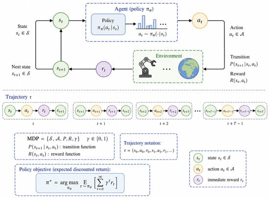
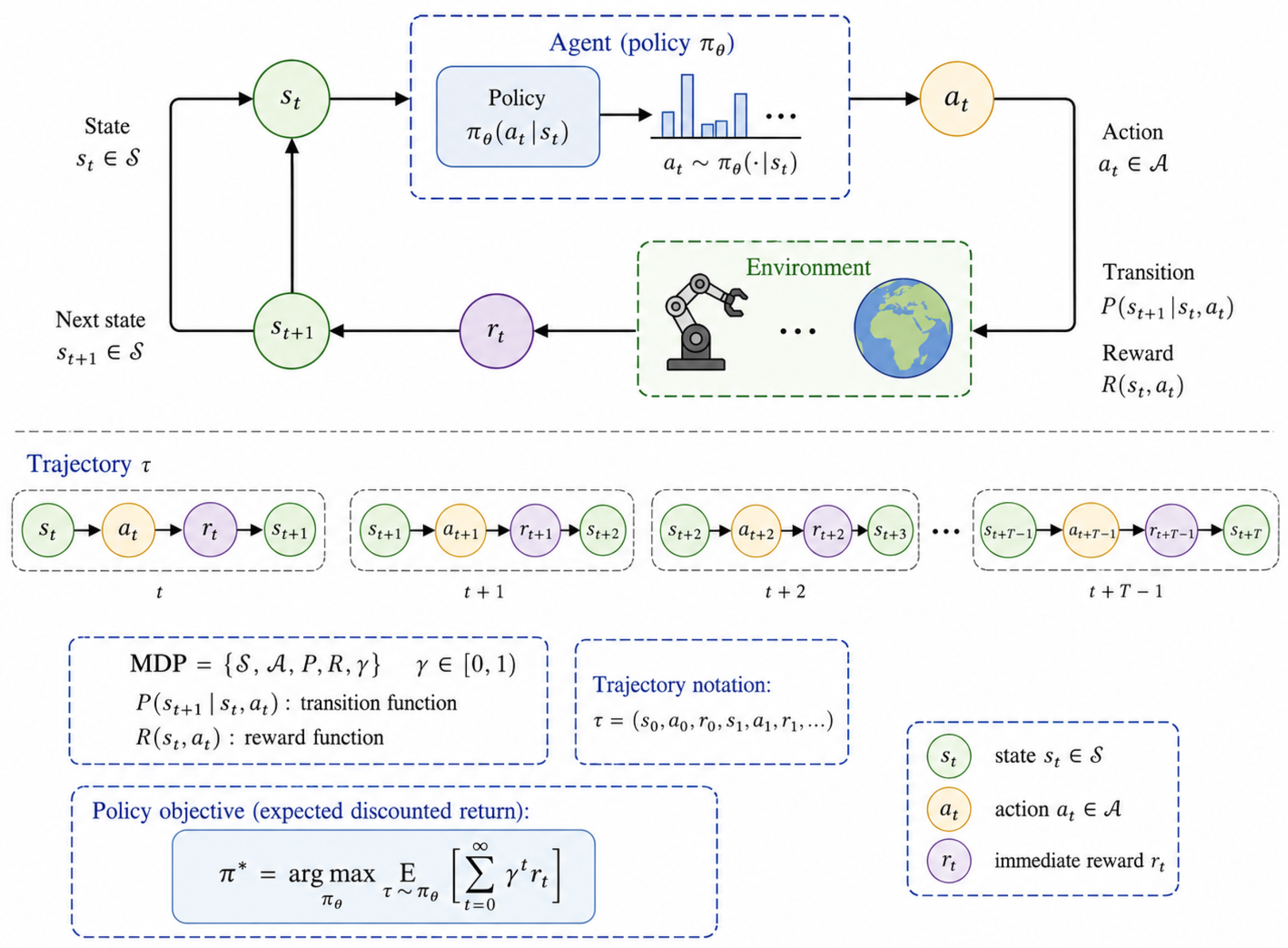
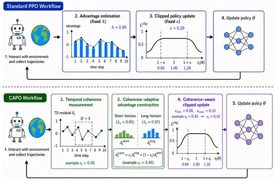
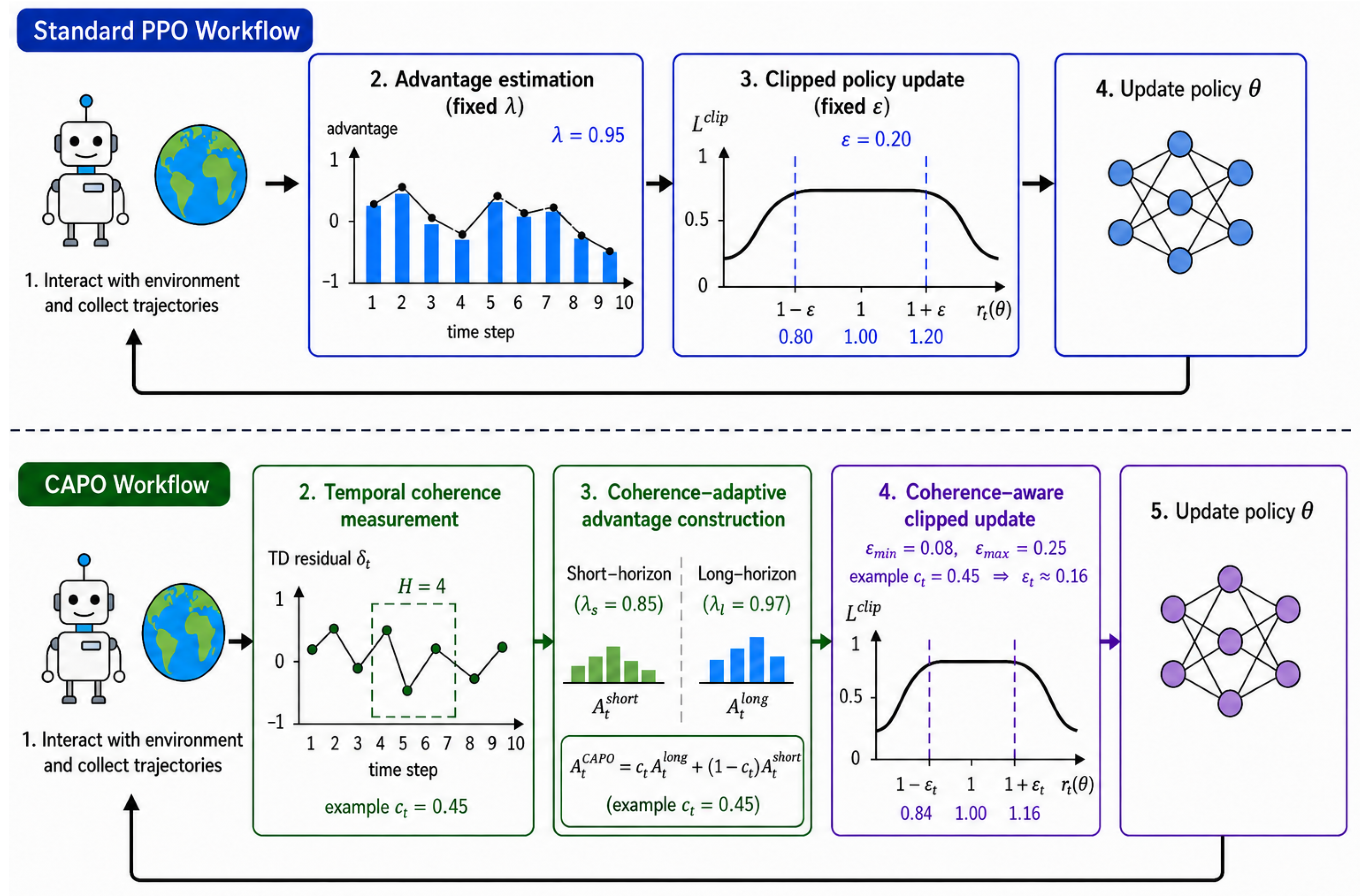
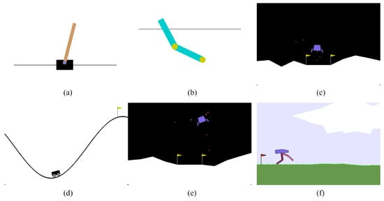
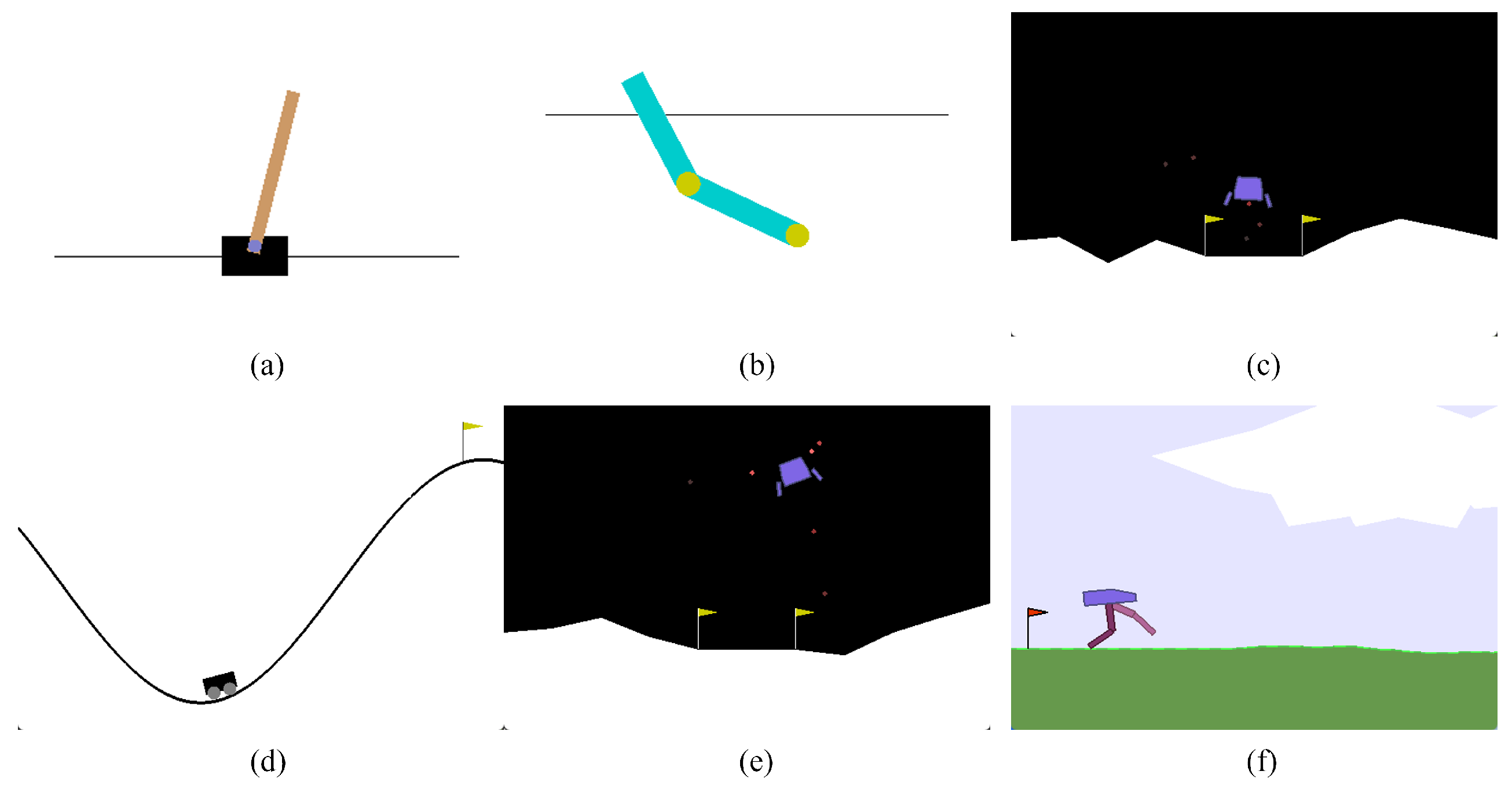
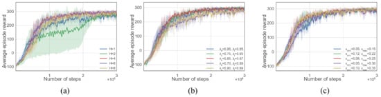
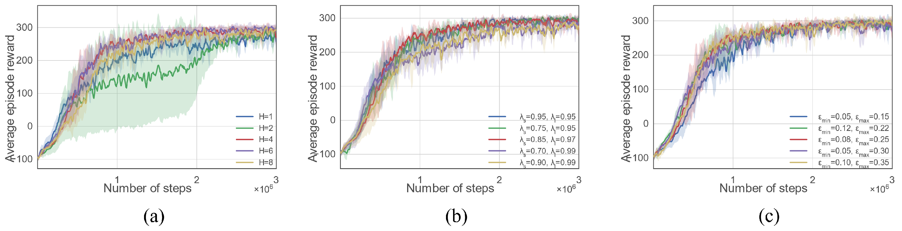
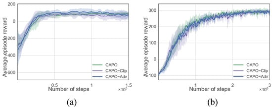
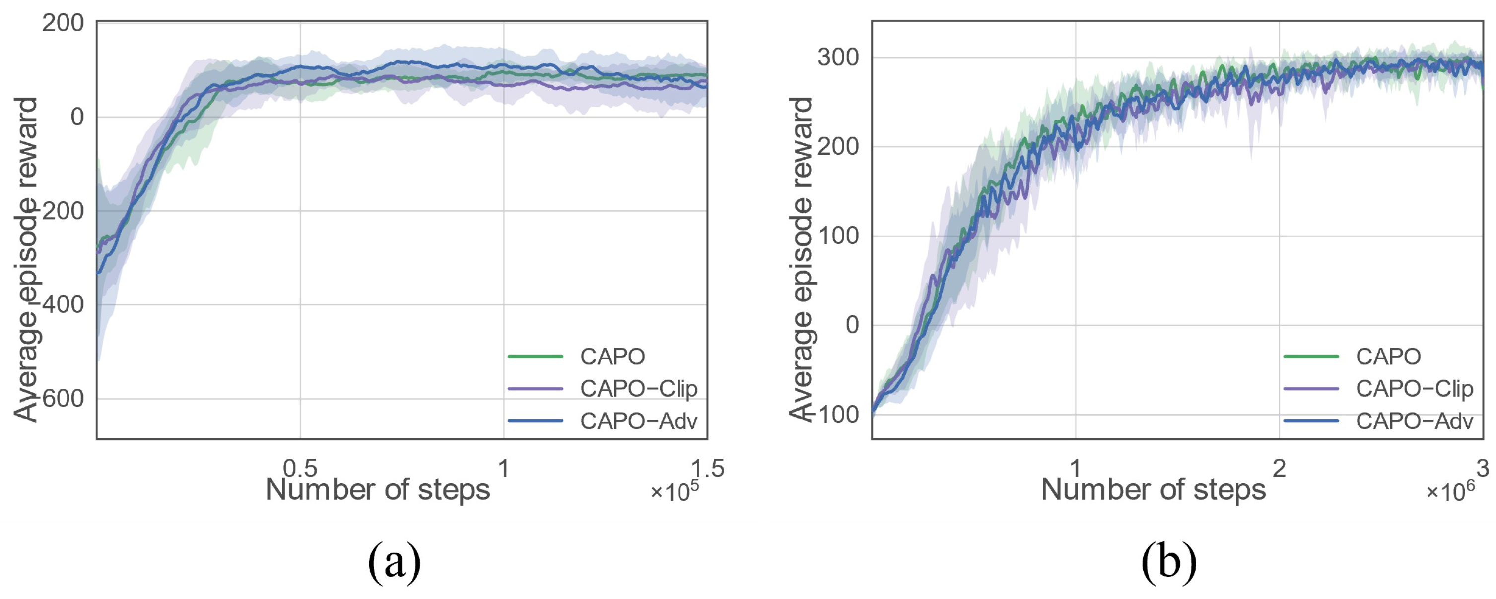
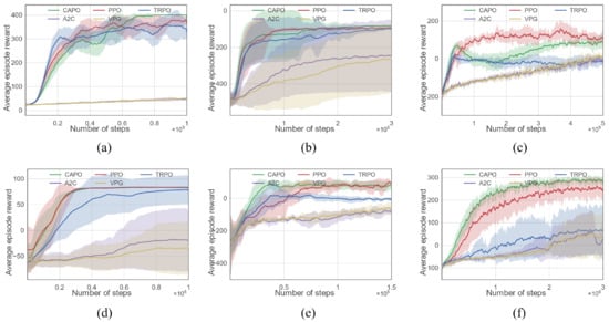
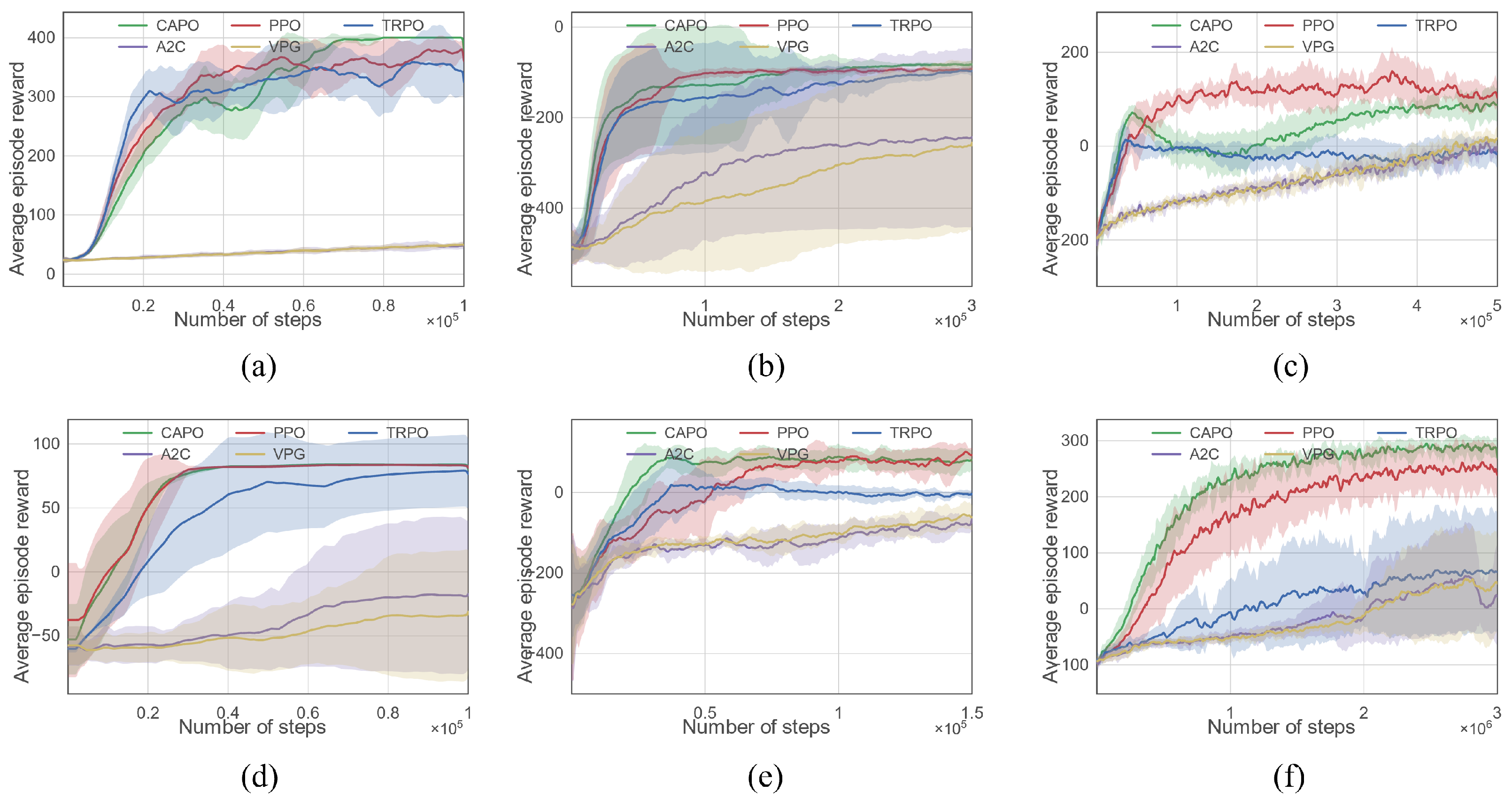

Disclaimer/Publisher’s Note: The statements, opinions and data contained in all publications are solely those of the individual author(s) and contributor(s) and not of MDPI and/or the editor(s). MDPI and/or the editor(s) disclaim responsibility for any injury to people or property resulting from any ideas, methods, instructions or products referred to in the content. |
© 2026 by the authors. Licensee MDPI, Basel, Switzerland. This article is an open access article distributed under the terms and conditions of the Creative Commons Attribution (CC BY) license.