A Method for Compiling the Random Load Spectrum of the Main Shaft Torque of the Vertical Ring-Die Biomass Briquetting Machine Based on Kernel Density Estimation and Copula Function

Abstract

To address the strong variability, complex cyclic characteristics, and difficulty in characterizing the main shaft torque load of vertical ring-die biomass briquetting machines, this study proposes a random load spectrum generation method based on kernel density estimation (KDE) and a Copula function. The measured torque time-history signal was processed using wavelet-threshold denoising and rainflow counting to extract cycle mean and cycle amplitude samples. KDE was used to estimate their marginal distributions, and a Copula function was introduced to construct the joint distribution model. The random load spectrum was then reconstructed through two-dimensional probability integration based on the fitted joint density function. The results show that the Frank Copula best describes the dependence structure between the cycle mean and the cycle amplitude. The reconstructed load spectrum agrees well with the measured load spectrum in terms of marginal frequency distribution and main peak intervals, with an RMSE of 6.3161 and an NRMSE of 6.94%. Compared with the KDE-independent baseline model, the proposed KDE–Frank Copula model reduces the RMSE by 12.74%. These results indicate that the proposed method can effectively characterize the statistical features of the random torque load of the main shaft and provide methodological support for load spectrum generation, fatigue life prediction, and reliability design of vertical ring-die biomass briquetting machines.

1. Introduction

The rapid development of global large-scale livestock farming has not only brought economic benefits to rural and pastoral areas but also caused serious environmental pollution problems [1]. Since the 21st century, global biomass densification technology has gradually shifted from a single fuel production mode to an integrated solution combining energy utilization and environmental protection [2]. Research and development in developed countries mainly focuses on high-value-added products and automation technologies, whereas developing countries place greater emphasis on the popularization of low-cost and highly applicable technologies [3]. As global biomass densification technology transitions towards the integration of energy utilization and environmental protection, vertical ring-die biomass briquetting machines play a crucial role in promoting the resource utilization of rural waste and supporting the sustainable development of the livestock industry.

The working environment of vertical ring-die biomass briquetting machines is complex, and the operating conditions are highly variable, which directly leads to significant non-stationary characteristics in the working loads of their core components. Investigating the working load characteristics and load distribution patterns of core components under actual briquetting conditions is essential for accurately reconstructing the service load history of the equipment. It also provides an important basis for identifying the causes of component failure and conducting stability design assessment and structural reliability evaluation [4,5,6].

The rainflow counting method is the core approach for load spectrum compilation and fatigue analysis [7,8,9], enabling the construction of mean–amplitude two-dimensional load spectra and fatigue assessment in conjunction with Miner’s theory [7,8]. It is often accompanied by preprocessing steps such as outlier elimination to enhance engineering applicability [9]. Kernel density estimation (KDE) is a nonparametric probability density estimation method that does not require a predefined distribution form and can flexibly describe complex data distribution characteristics. Therefore, it has been widely applied in load statistics, reliability analysis, and prognostics and health management (PHM). Among these studies, Hu et al. used KDE to fit the wind speed probability density function, verifying the flexibility and accuracy of this method [10]; Duda et al. proposed recursive KDE and proved its convergence [11]; Sidibé et al. used KDE to estimate the system reliability function and analyzed the impact of kernel smoothing parameters on the cost model [12]; Wang et al. proposed a KDE method adapted to high-speed train vibration data [13]; Wang et al. introduced KDE into robust random configuration networks, reducing outlier interference with the model [14]; Zhang et al. proposed a nonlinear KDE method that enhances anomaly discrimination [15].

The combination of Copula functions and KDE has been widely used in modeling multivariate correlation structures. Xu et al. constructed a wind farm output correlation model, improving the accuracy of correlation structure characterization [16]; Wang et al. described nonlinear correlations among components using Copulas, optimizing the reliability analysis method [17]; Zhang et al. established a joint model of multiple performance degradation parameters to achieve comprehensive reliability assessment of the electric spindle [18]; Bao et al. constructed a Copula model for wind speed and blade load and used it for load prediction [19]; Cui et al. combined KDE and Copulas to depict the coupling relationship between wind and power generation, generating joint scenarios [20]; Gao et al. used KDE to fit the measured load spectrum of the bogie, breaking through the limitations of traditional parametric models [21]. Copula-based methods have also been applied to photovoltaic carrying capacity eval-uation and wind farm power modeling [22,23]. Meanwhile, KDE-based methods have been used for load or stress spectrum extrapolation in fuel cell buses, cranes, structural frames, and machining center spindles [24,25,26,27].

Despite these advances, several limitations remain in the application of these methods to the load characterization of agricultural machinery. First, most existing studies focus on noise reduction of conventional mechanical vibration signals and single-variable load statistics, whereas joint modeling research on the measured random torque load of agricultural machinery remains insufficient. Second, the systematic analysis of the marginal distribution characteristics of cycle mean and cycle amplitude and their dependence structure remains limited. Third, due to the heterogeneous nature of biomass materials and the fluctuation of the briquetting process, the measured main shaft torque load exhibits obvious non-Gaussian and non-stationary characteristics. Therefore, traditional parametric models struggle to accurately capture the complex statistical characteristics of measured loads.

In this study, the measured torque signal of the main shaft of a vertical ring-die biomass briquetting machine was taken as the research object. After wavelet-threshold denoising, the load cycle mean and amplitude were extracted using the rainflow counting method. A nonparametric joint modeling framework based on KDE and Copula functions was then introduced to characterize the marginal distribution characteristics and dependence structure of the main shaft torque load. The main contribution of this study lies in extending the KDE–Copula joint modeling strategy to the measured main shaft torque load of a vertical ring-die biomass briquetting machine, thereby providing a data-driven basis for two-dimensional load spectrum construction and subsequent fatigue life assessment and reliability analysis. This approach enables a more flexible description of the non-Gaussian and non-stationary characteristics of the measured torque load and improves the representation of the two-dimensional load spectrum. The results provide theoretical and data support for load spectrum compilation, fatigue life assessment, and structural reliability design of the main shaft of the vertical ring-die biomass briquetting machine.

2. Load Measurement of the Vertical Ring-Die Biomass Briquetting Machine

2.1. Overall Workflow of the Proposed Method

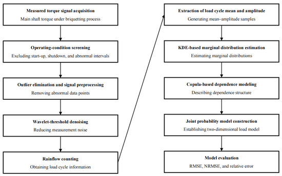
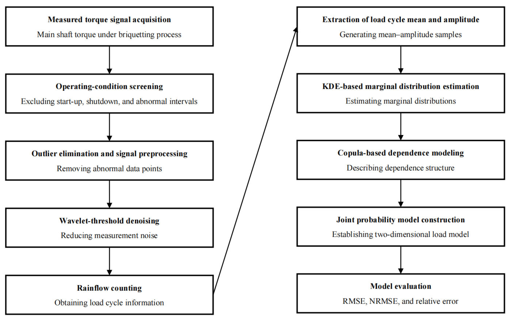
To improve the readability of the proposed method and clarify the role of each equation, the complete procedure for measured main shaft torque load modeling is summarized in Figure 1. The procedure begins with the acquisition and screening of measured torque signals, followed by signal preprocessing, load feature extraction, marginal distribution esti-mation, dependence structure modeling, and model evaluation.

Figure 1. Flowchart of the proposed joint modeling procedure for measured main shaft torque loads.

First, the torque signal of the main shaft is measured under actual briquetting conditions. To ensure the validity of the measured data, unstable operating periods, such as machine start-up, shutdown, and abnormal fluctuation intervals, are excluded. Only the torque signal segments corresponding to relatively stable operating conditions are retained for subsequent analysis. Second, outlier elimination and wavelet-threshold denoising are performed to reduce the influence of measurement noise and abnormal data points. Third, the rainflow counting method is used to transform the preprocessed time-domain torque signal into load cycle information, from which the load cycle mean and amplitude are extracted. Fourth, KDE is applied to estimate the marginal probability distributions of the load cycle mean and amplitude without assuming a predefined distribution form. Fifth, Copula functions are introduced to describe the dependence structure between the load cycle mean and amplitude, and a joint probability model of the measured main shaft torque load is established. Finally, the accuracy and applicability of the proposed model are evaluated using RMSE, NRMSE, and relative error.

2.2. Test Principle and Equipment

The vertical ring-die biomass briquetting machine conveys raw materials, including cow dung, into the dedicated ring-die structure. The compression components apply pressure, causing the materials to solidify within the mold and form fuel briquettes. The main shaft torque load is an important parameter that affects the quality of the briquettes, the energy consumption of the equipment, and the service performance of key components. Accurate acquisition of this parameter is of great significance for optimizing the structure of the vertical ring-die biomass briquetting machine, matching the operating parameters, and evaluating the fatigue life.

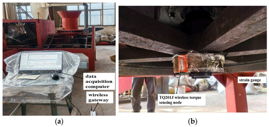
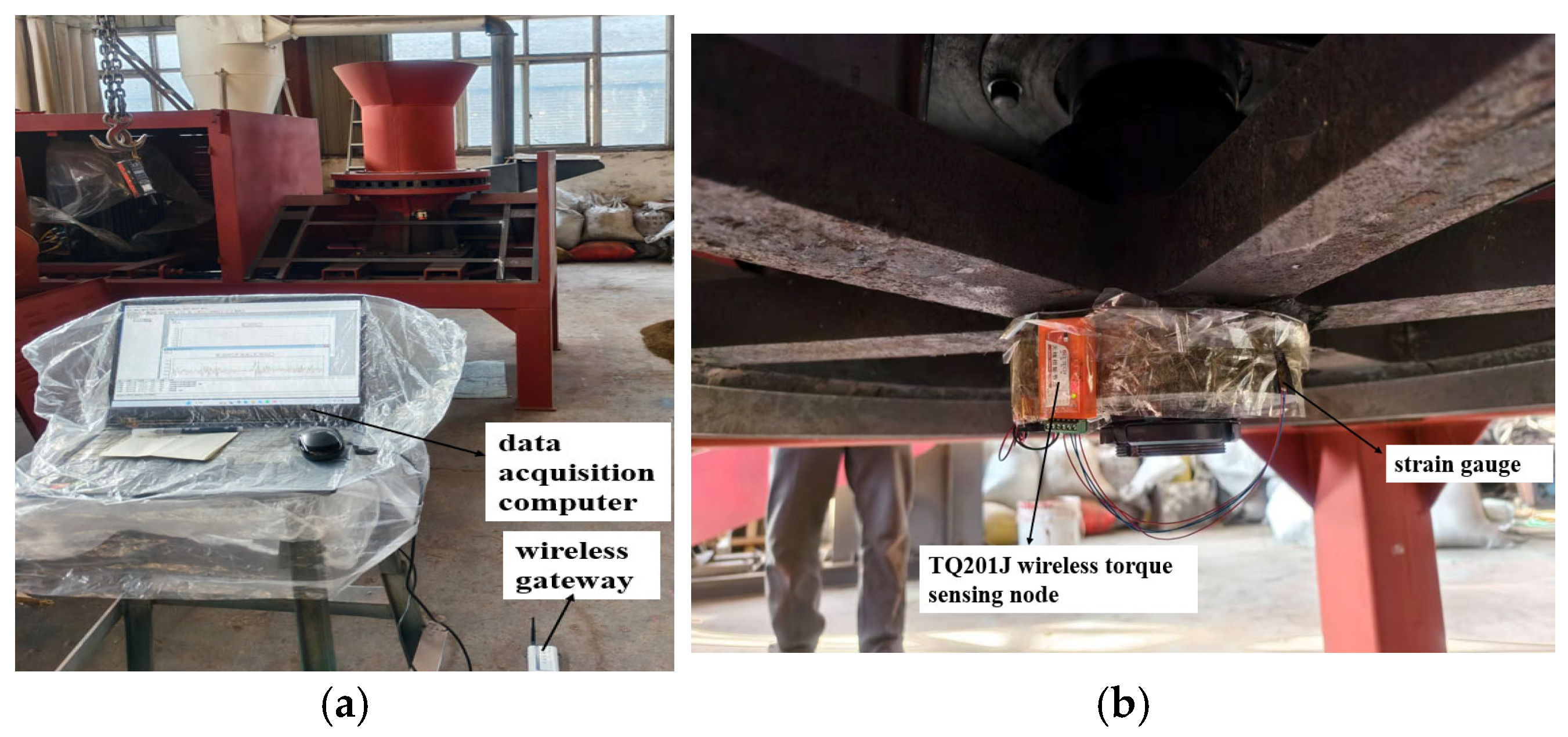
A prototype of a vertical ring-die biomass briquetting machine with a production capacity of approximately 1.5 tons per hour was used for load testing. The testing equipment included a TQ201J wireless torque sensing node, a BS951-T wireless gateway, a data acquisition computer, and other devices for production experiments. The test employed the full-bridge measurement method to capture physical deformation information on the main shaft surface. Compared with the half-bridge measurement method, the full-bridge configuration offers higher sensitivity and measurement accuracy and effectively eliminates the influence of temperature-induced resistance changes, bending strain, and axial (tensile/compressive) strain on the results. The sampling frequency was set to 100 Hz, and the sampling duration was 100 s. The test signal was transmitted via the wireless gateway to the data acquisition com-puter and, in conjunction with the dedicated BeeData data acquisition software (ver-sion V18.7), enabled real-time data tracking and recording.

Due to the tight structural configuration of the vertical ring-die biomass briquetting machine and the lack of exposed surfaces on the main shaft, an equivalent measurement approach was adopted to capture the main shaft torque load. Given that the driving large pulley is rigidly coupled to the main shaft via a key connection, the two components exhibit high synchronicity in torsional dynamics; thus, the torsional deformation on the pulley surface faithfully reflects the actual loading state of the main shaft.

The layout of the torque measurement system and the strain-gauge installation are shown in Figure 2. Figure 2a shows the test prototype, and Figure 2b shows the strain-gauge placement on the torque sensing node.

Figure 2. Torque measurement system and strain-gauge installation: (a) test prototype; (b) strain-gauge placement on the torque sensing node.

2.3. Working Principle of the Vertical Ring-Die Biomass Briquetting Machine

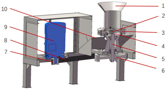
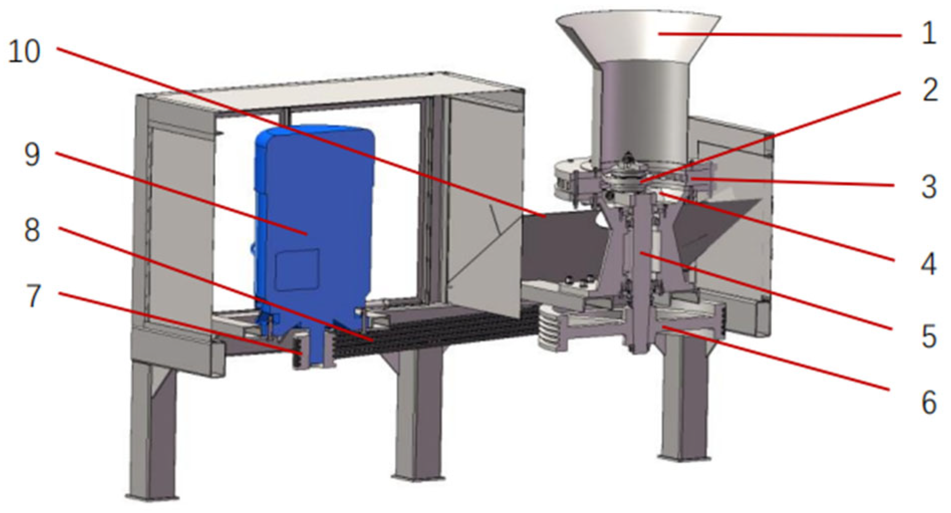
The vertical ring-die biomass briquetting machine comprises a feed hopper, a transmission mechanism, a compaction chamber, and a discharge area, as shown in Figure 3. First, cow dung is pre-treated using a grinder and then conveyed to the feed hopper via a conveyor belt before entering the compaction chamber for compaction. Under the action of the pressure rollers and cutters, the material enters the ring-die holes. As a continuous stream of material is pressed into the ring-die holes, rectangular briquettes are formed.

Figure 3. Sectional view of the vertical ring-die biomass briquetting machine: 1—feed hopper; 2—pressing roller; 3—ring die; 4—hinge cutter; 5—main shaft; 6—large pulley; 7—small pulley; 8—belt; 9—motor; 10—discharge plate.

2.4. Main Shaft Torque Signal Acquisition and Preprocessing

Considering the complexity of the operating environment, torque signal acquisition inevitably involves outliers, which directly impair the accuracy of signal analysis and load spectrum compilation. To mitigate the influence of measurement noise and random interference on torque signal analysis, this paper applies a soft thresholding function to the wavelet decomposition coefficients to obtain a torque time-history signal that more accurately reflects actual operating conditions. The soft thresholding function sets coefficients with absolute values below the threshold to zero and shrinks those with absolute values above the threshold toward zero by an amount equal to the threshold, thereby suppressing noise while preserving the signal’s dominant transient features. Its mathematical expression is:

$$\widehat{w}=\left\{\begin{array}{cc}sgn(w)(\left|w\right|-\lambda ),& \left|w\right|\ge \lambda \\ 0,& \left|w\right|<\lambda \end{array}\right.$$

(1)

where $w$ denotes the original wavelet coefficient, $\widehat{w}$ denotes the processed wavelet coefficient, and $\lambda$ is the threshold. Compared with the hard thresholding function, the soft thresholding function exhibits superior continuity and mitigates local oscillations in the reconstructed signal, albeit introducing a certain degree of amplitude bias.

The number of wavelet decomposition levels is set to 3. Considering the torque signal sampling frequency of 100 Hz in this study, a three-level wavelet decomposition yields one low-frequency approximation component and three high-frequency detail components. This effectively separates high-frequency noise components while avoiding over-decomposition, which could otherwise lead to loss of load-related information.

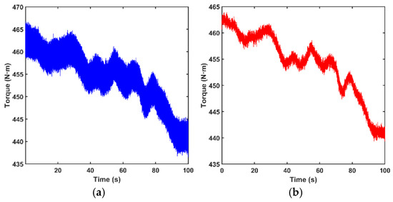
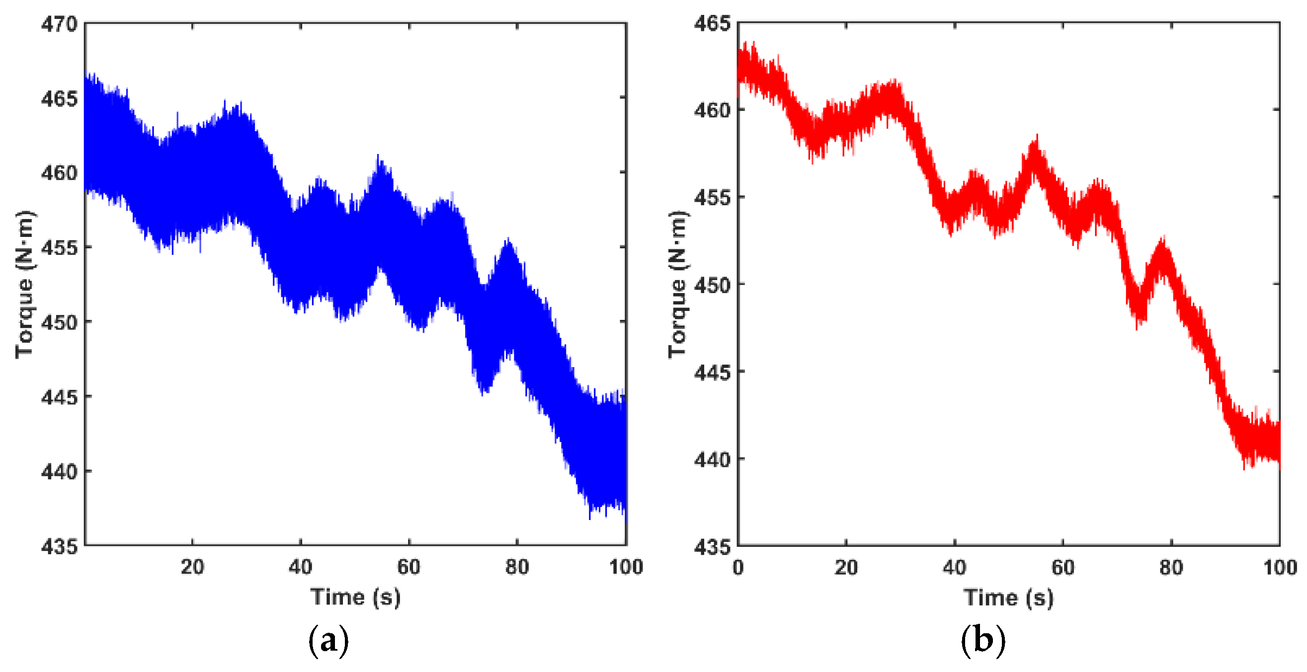
As shown in Figure 4, after wavelet-threshold denoising, local high-frequency disturbances in the main shaft torque signal have been effectively suppressed, while the dominant load variation trend has been preserved. The processed torque load fluctuates around 454 N·m, with a relatively small overall amplitude, indicating that the main shaft torque output under this test condition is comparatively stable.

Figure 4. Time-domain curves of the main shaft torque of the vertical ring-die biomass briquetting machine: (a) original main shaft torque; (b) processed main shaft torque.

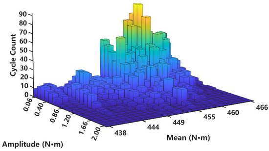
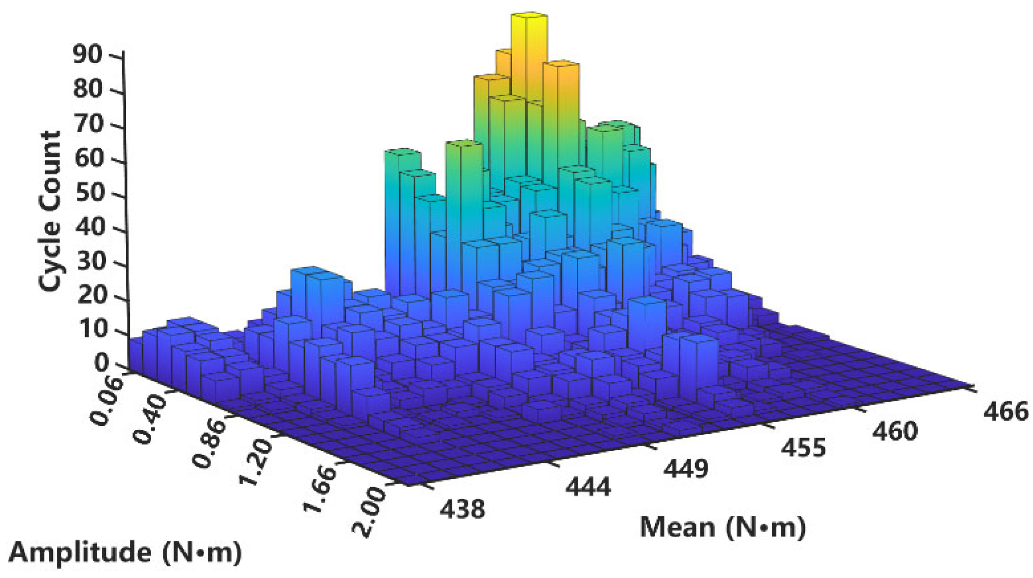
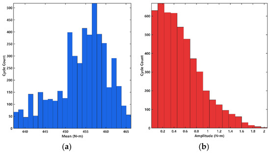
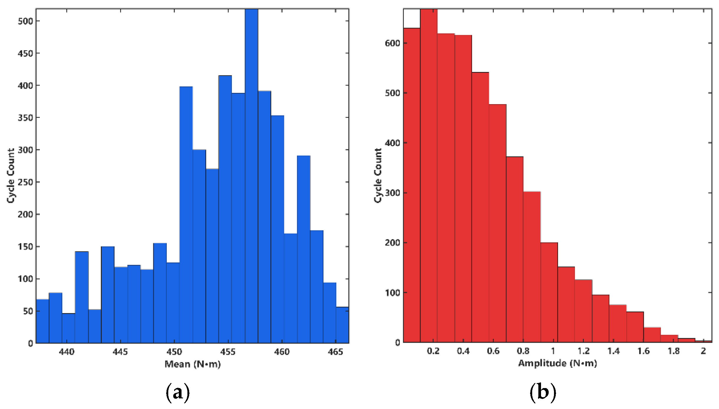
After torque signal preprocessing, the four-point rainflow counting algorithm is applied to perform cycle identification and frequency statistics on the processed dataset. A three-dimensional rainflow matrix—with 24 mean bins and 18 amplitude bins—and a two-dimensional frequency histogram are constructed, as shown in Figure 5 and Figure 6. The cycle mean of the main shaft torque is predominantly concentrated around 455 N·m, exhibiting a unimodal distribution. Meanwhile, the cycle amplitude is strongly concentrated in the low-amplitude range of 0–1.0 N·m. This statistical pattern carries clear engineering and physical significance: under normal consolidation and forming conditions, the main shaft of the vertical ring-die biomass briquetting machine sustains a high, nearly constant baseline extrusion torque. However, the amplitude of alternating loads—induced by uneven material feed or mechanical vibration—remains relatively small, confirming that the extrusion mechanism’s transmission and output operate in a comparatively stable state.

Figure 5. Three-dimensional rainflow matrix of the main shaft torque. The color gradient represents the magnitude of cycle count, with warmer colors indicating higher cycle counts.

Figure 6. Two-dimensional frequency histograms of the rainflow-counted torque cycles: (a) cycle mean; (b) cycle amplitude.

3. Measured Torque Rainflow Statistics and Independence Test

3.1. Rainflow Counting and Load Spectrum Statistics

During the pressing test of the vertical ring-die biomass briquetting machine, the measured main shaft torque signal exhibits pronounced discreteness, randomness, and large-sample characteristics. The raw time-domain data are unsuitable for direct use in load pattern recognition and fatigue analysis. Therefore, statistical processing and feature extraction must be performed on the test load to transform complex random loads into engineering-useful load spectra. For this highly random loading condition, this paper employs the rainflow counting method to conduct cycle-based statistical analysis of the torque time history, converting the complex random load signal into a statistical representation comprising cycle mean, cycle amplitude, and their corresponding frequencies—thereby extracting effective load information that reflects actual service conditions.

3.2. Mean–Amplitude Independence Test

To assess whether the cycle mean and cycle amplitude satisfy the independence assumption required for rainflow-based parameter extrapolation, an independence test is conducted for both variables. Based on the chi-square test of independence for contingency tables, under the null hypothesis H₀: “the cycle mean and cycle amplitude are independent”, the test statistic is given by Equation (2) and asymptotically follows a chi-square distribution with degrees of freedom (r − 1)(s − 1).

$${\chi }^2=k{{\displaystyle \sum _{i=1}^r{\displaystyle \sum _{j=1}^s\left(k_{ij}-k_i{k}_j{k}^{-1}\right)}}}^2/k_i{k}_j$$

(2)

where $k$ denotes the total sample size; $k_i$ denotes the frequency of the cycle amplitude at the $i-th$ level; $k_j$ denotes the frequency of the cycle mean at the $j-th$ level; and $k_{ij}$ denotes the frequency of rainflow cycles falling simultaneously into the $i-th$ cycle amplitude level and the $j-th$ cycle mean level.

Using MATLAB(R2024a) software and based on 4989 valid samples, a stratified sampling method was employed to construct a contingency table for the independence test. The calculated chi-square statistic was 1357.97—substantially exceeding the critical value of 438.11 at the 0.05 significance level (p < 0.001). This indicates a statistically significant dependence between the cycle mean and cycle amplitude; consequently, their two-dimensional joint distribution cannot be approximated as the product of the marginal distributions. It should be noted that even if the absolute values of linear correlation coefficients—such as Pearson’s or Spearman’s—are relatively small in subsequent analyses, this does not preclude the presence of stable nonlinear dependencies or non-Gaussian correlation structures between the variables. Therefore, this paper further employs the kernel density estimation (KDE) method to estimate the marginal distributions and integrates a Copula function to construct a joint distribution model, thereby accurately characterizing the complex dependence structure between the two variables.

4. Kernel Density Estimation and Copula-Based Joint Distribution Modeling

4.1. Estimation of the Marginal Distributions of the Cycle Mean and Amplitude

After denoising and rainflow counting, the extracted cycle mean and cycle amplitude, respectively, characterize the load’s baseline level and fluctuation intensity, jointly influencing the structural fatigue response. As these rainflow parameters often exhibit complex statistical features—including skewness, multimodality, and heavy tails—traditional parametric models (e.g., the normal or Weibull distribution) frequently fail to accurately capture their underlying distributions. Therefore, this paper employs kernel density estimation (KDE) to perform nonparametric modeling of the marginal distributions of the cycle mean and cycle amplitude.

Suppose the samples $X_1,X_2,\dots ,X_n$ come from an unknown continuous distribution, then the kernel density estimation can be expressed as:

$${\widehat{f}}_n(x)={\displaystyle \frac{1}{nh}}{\displaystyle \sum _{i=1}^{n}K\left(\frac{x-X_i}{h}\right)}$$

(3)

where $K(\cdot )$ denotes the kernel function, $h$ is the bandwidth, and $n$ is the sample size. This paper adopts the Gaussian kernel function as:

$$K(u)={\displaystyle \frac{1}{\sqrt{2\pi }}}\exp \left(-{\displaystyle \frac{u^2}{2}}\right)$$

(4)

The bandwidth is automatically selected using the normal reference rule. To enhance robustness against skewed distributions and outliers, the scale parameter in the bandwidth calculation is set to the smaller of the sample standard deviation and the interquartile range–based scale. This approach achieves an effective balance between smoothness and preservation of local features, thereby improving the stability and applicability of the marginal distribution estimation.

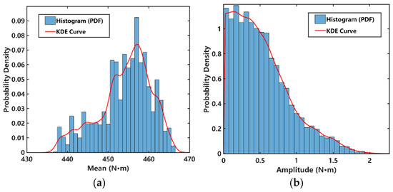
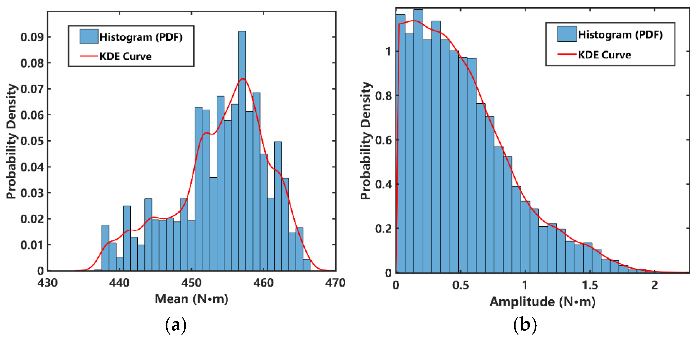
Based on the above methodology, the marginal densities of the cycle mean and cycle amplitude samples were estimated separately, and the fitting results were compared and analyzed against the corresponding sample histograms. The results show that, as illustrated in Figure 7, the KDE curve exhibits high fidelity to the sample histogram in terms of main peak location, distribution skewness, and tail behavior. Compared with traditional parametric fitting, KDE requires no prior assumption about the underlying distribution form and demonstrates superior adaptability to local fluctuations. Specifically, the cycle mean is highly concentrated in the range of 450–462 N·m (with a peak near 455–458 N·m), exhibiting a nonuniform aggregation pattern with discernible local fluctuations; in contrast, the cycle amplitude is concentrated within 0–1.5 N·m, and its probability density decreases monotonically with increasing amplitude—characteristic of a heavy-tailed, right-skewed distribution. This indicates that, under actual operating conditions, small-amplitude cycles predominate, whereas low-frequency, large-amplitude cycles—though more damaging to fatigue life—retain significant engineering relevance.

Figure 7. Kernel-density-estimated marginal probability density functions: (a) cycle mean; (b) cycle amplitude.

Overall, the marginal distributions of the cycle mean and cycle amplitude—obtained via kernel density estimation—accurately capture the statistical characteristics of the rainflow cycle samples, thereby providing a reliable basis for subsequent mean–amplitude correlation analysis and Copula-based joint distribution modeling.

4.2. Joint Statistical Analysis of the Cycle Mean and Cycle Amplitude

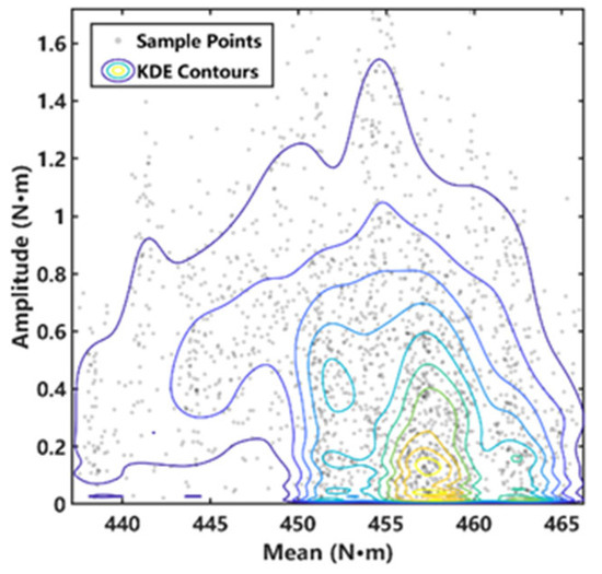
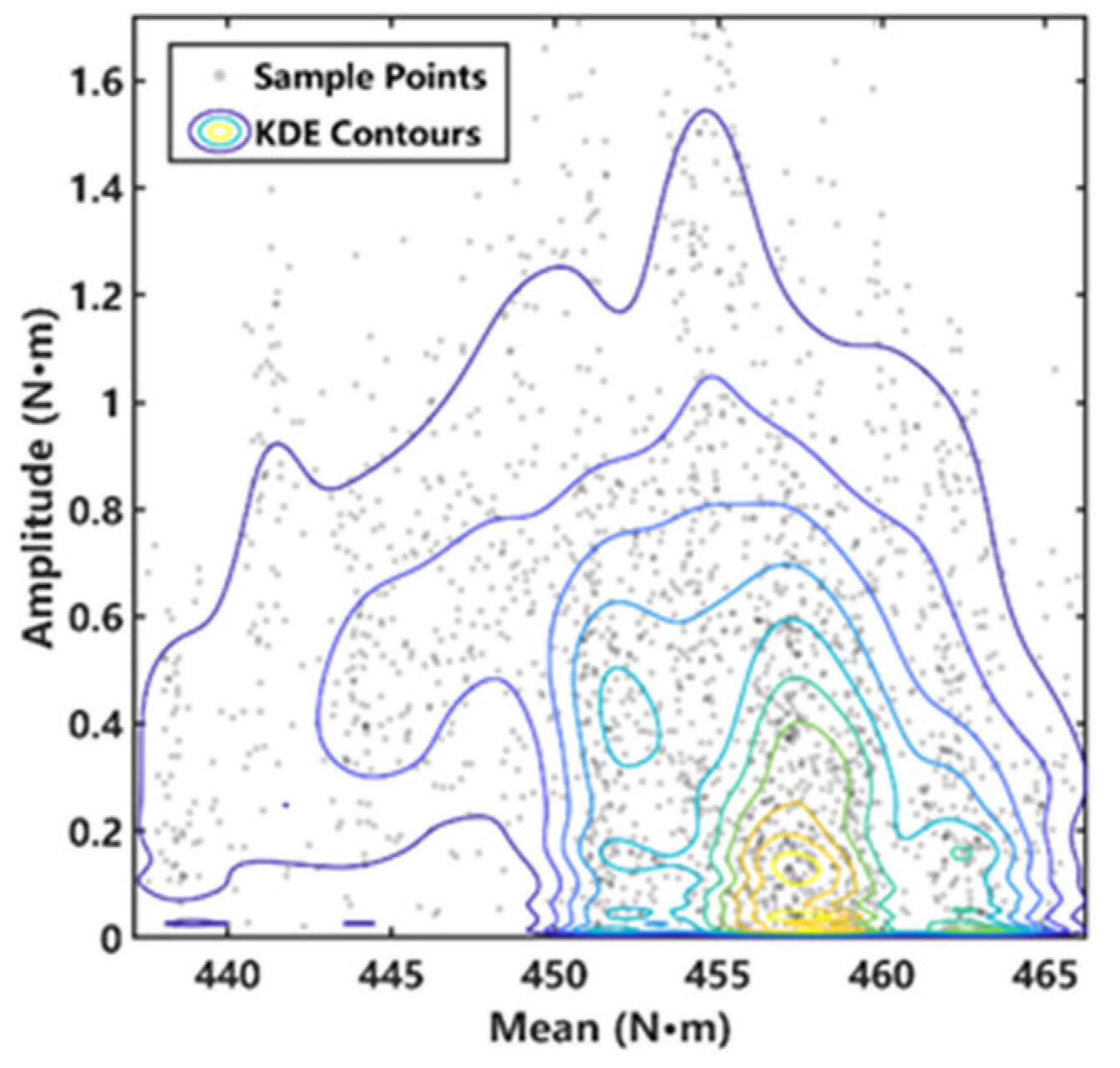
To reveal the coupling distribution pattern between the cycle mean and cycle amplitude in rainflow cycles, joint statistical analysis was performed by combining scatter plots, two-dimensional kernel density estimation, and correlation metrics. A scatter visualization of the cycle mean–amplitude data was conducted, and two-dimensional kernel density contour lines were superimposed, as shown in Figure 8.

Figure 8. Scatter plot and two-dimensional kernel density contour map of the mean–amplitude rainflow cycles.

Based on the scatter distribution, two-dimensional kernel density estimation was used to smooth and model the joint statistical behavior of the cycle mean and cycle amplitude. Let $M$ denote the cycle mean and $A$ denote the cycle amplitude. For the sample set ${\{(M_i,A_i)\}}_{i=1}^n$, the two-dimensional kernel density estimation can be generally expressed as:

$${\widehat{f}}_{M,A}(m,a)={\displaystyle \frac{1}{n{h}_M{h}_A}}{\displaystyle \sum _{i=1}^{n}K}\left({\displaystyle \frac{m-M_i}{h_M}}\right)K\left({\displaystyle \frac{a-A_i}{h_A}}\right)$$

(5)

where ${\widehat{f}}_{M,A}(m,a)$ denotes the estimated joint probability density of the cycle mean $M$ and cycle amplitude $A$; $h_M$ and $h_A$ are the bandwidths in the mean and amplitude directions, respectively; $K(\cdot )$ is the kernel function; and $n$ is the sample size. Because the cycle amplitude is a strictly positive variable and is highly concentrated in the low-amplitude region, direct KDE in the original amplitude space may produce boundary bias near zero. Therefore, the amplitude variable $A$ is transformed into the logarithmic variable $Z$:

$$Z=\ln A,A>0$$

(6)

This transformation compresses the right-skewed amplitude distribution and improves the stability of kernel density estimation.

In this study, KDE is first performed in the transformed space $(M,Z)$. The joint density estimated in the transformed mean–log-amplitude space is denoted as:

$${\widehat{f}}_{M,Z}(m,z)={\displaystyle \frac{1}{n{h}_M{h}_Z}}{\displaystyle \sum _{i=1}^{n}K}\left({\displaystyle \frac{m-M_i}{h_M}}\right)K\left({\displaystyle \frac{z-Z_i}{h_Z}}\right)$$

(7)

where $Z_i=\ln A_i$, $A_i$ is the cycle amplitude of the $i-th$ rainflow cycle sample, and $h_z$ is the bandwidth in the logarithmic amplitude direction.

However, since the density is estimated in the transformed variable space $(M,Z)$, it must be converted back to the original physical variable space $(M,A)$. According to the probability density transformation rule, the joint density in the original mean–amplitude space is obtained by multiplying the density in the transformed space by the absolute value of the Jacobian term:

$${\widehat{f}}_{M,A}(m,a)={\widehat{f}}_{M,Z}(m,\ln a)\left|{\displaystyle \frac{\partial z}{\partial a}}\right|$$

(8)

Since $z=\ln a$, the derivative is:

$$\left|{\displaystyle \frac{\partial z}{\partial a}}\right|={\displaystyle \frac{1}{a}}$$

(9)

Therefore, the joint probability density in the original mean–amplitude space can be expressed as:

$${\widehat{f}}_{M,A}(m,a)={\displaystyle \frac{{\widehat{f}}_{M,Z}(m,\ln a)}{a}},a>0$$

(10)

The Jacobian correction ensures that the total probability remains unchanged before and after the variable transformation. In other words, the logarithmic transformation improves the stability of density estimation in the low-amplitude region, while the Jacobian correction guarantees that the reconstructed density remains physically meaningful in the original cycle mean–amplitude space.

Figure 8 shows the scatter plot and two-dimensional kernel density contour map of the mean–amplitude rainflow cycles. The joint distribution of the cycle mean and cycle amplitude exhibits pronounced nonuniformity, characterized by a dominant central peak, surrounding secondary peaks, and sparse tail expansion. The system’s dynamic response is dominated by very small-amplitude cycles below 1.0 N·m occurring at relatively high mean levels, with the core region located at approximately 454 N·m. Large-amplitude cycles, which may be more critical to fatigue damage, appear only as sparse isolated points.

The Pearson and Spearman correlation coefficients between the cycle mean and cycle amplitude are −0.1619 and −0.2328, respectively, indicating a weak global negative association. However, considering both the formal independence test and the nonuniform aggregation pattern shown in the two-dimensional density contour, the cycle mean and cycle amplitude still exhibit statistically significant nonlinear dependence in the probability space. Therefore, it is necessary to further introduce a Copula function to characterize the dependence structure between the two variables rather than simply assuming that they are independent.

4.3. Preprocessing for Copula Modeling Based on KDE

After characterizing the joint distribution of the cycle mean and cycle amplitude, this paper performs nonparametric marginal distribution fitting and standardization preprocessing on the original samples prior to Copula modeling. The core idea is to first estimate the marginal cumulative distribution functions (CDFs) of the cycle mean and cycle amplitude using kernel density estimation (KDE), then map the original variables to the unit interval via probability integral transformation, and finally use rank-based pseudo-observations as input to the Copula model. Thus, parametric assumptions regarding the marginal distributions are minimized, and modeling emphasis is placed squarely on the dependence structure between the variables.

Let the marginal cumulative distribution functions of the cycle mean and cycle amplitude be denoted by $F_M(m)$ and $F_A(a)$, respectively. Then the corresponding marginal probability density functions are given by:

$$F_M(M)={\displaystyle {\int }_{-\infty }^m{f}_M}(t)dt,F_A(a)={\displaystyle {\int }_0^a{f}_A}(t)dt$$

(11)

Since the true marginal distribution is unknown, this paper employs kernel density estimation (KDE) for nonparametric estimation:

$${\widehat{F}}_M(m)={\displaystyle {\int }_{-\infty }^m{\widehat{f}}_M}(t)dt,{\widehat{F}}_A(a)={\displaystyle {\int }_0^a{\widehat{f}}_A}(t)dt$$

(12)

In the implementation, the cycle amplitude marginal distribution incorporates positive-support constraints and boundary corrections to mitigate bias in the zero-neighborhood density estimation.

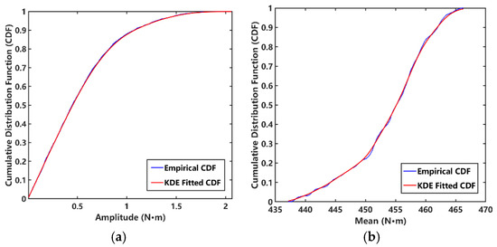
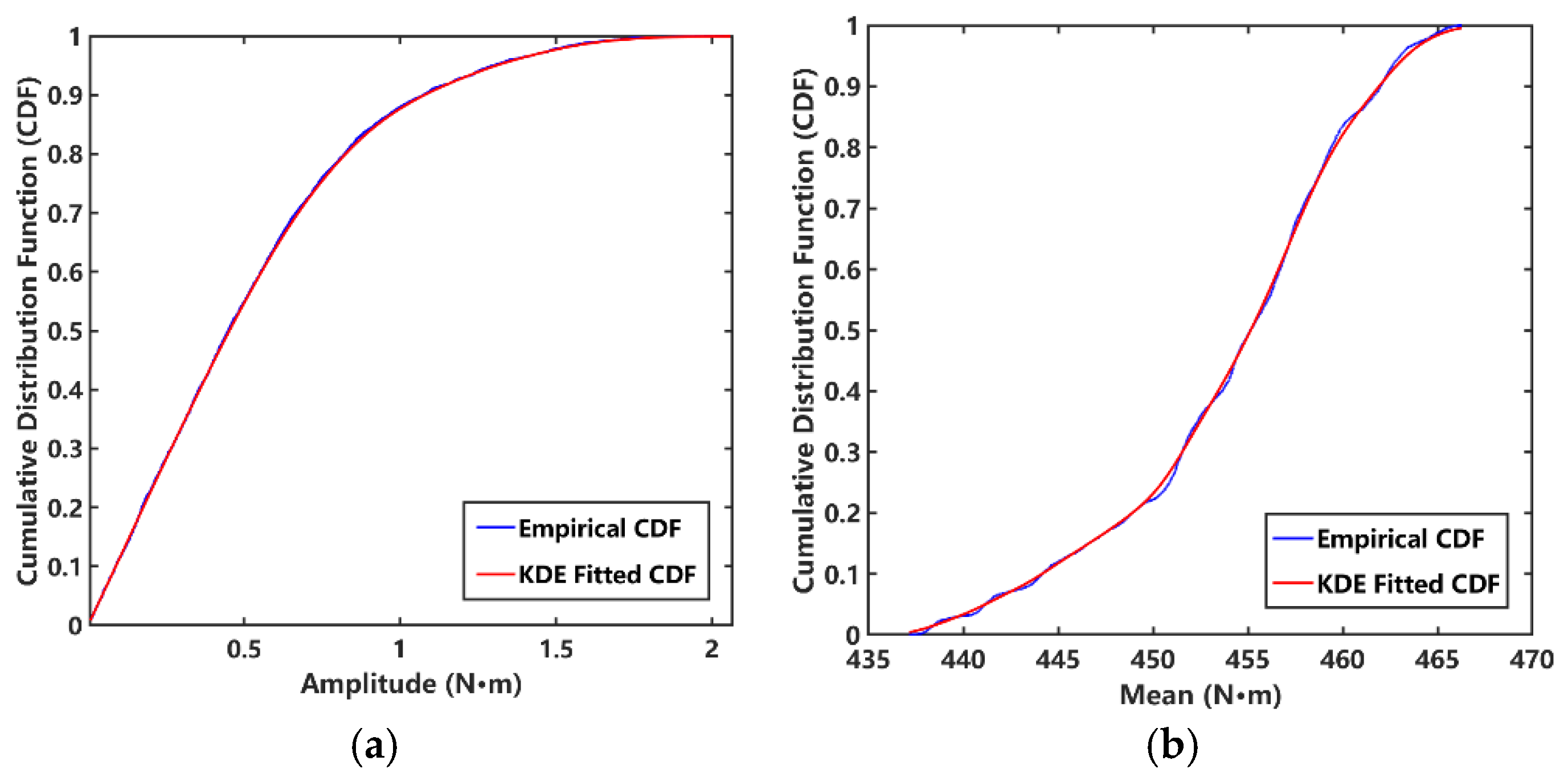
Figure 9a and Figure 9b present the empirical cumulative distribution functions (CDFs) and the kernel density estimation (KDE)-fitted CDFs for the cycle mean and cycle amplitude, respectively. Both plots show high overall agreement between the empirical and KDE-fitted CDFs, confirming that KDE-based marginal distribution modeling effectively preserves the statistical characteristics of the original samples. Specifically, the cycle amplitude marginal distribution exhibits a steep rise in the low-value region followed by progressive deceleration—reflecting pronounced concentration of low-amplitude cycles and right-skewed tail extension. In contrast, the cycle mean marginal distribution displays a relatively smooth cumulative growth, indicating that the cycle mean is predominantly concentrated within the primary operational interval. These results validate the reasonableness and effectiveness of using KDE to estimate marginal distributions prior to Copula modeling.

Figure 9. Kernel-density-estimated cumulative distribution functions: (a) cycle mean; (b) cycle amplitude.

After obtaining the marginal distribution function, a probability integral transformation is applied to the original sample:

$$U_i={\widehat{F}}_M(M_i),V_i={\widehat{F}}_A(A_i),i=1,2,\dots n.$$

(13)

This transformation maps the marginal information from the original physical variable space to the unit interval [0, 1], thereby decoupling the marginal distributions from the dependence structure and enabling the Copula model to focus exclusively on the association and coupling between the cycle mean and cycle amplitude. Because engineering samples may contain duplicate values and boundary points may yield unstable rank-based estimates, this paper adopts a rank-based pseudo-observation construction method:

$$u_i={\displaystyle \frac{rank(M_i)}{n+1}},v_i={\displaystyle \frac{rank(A_i)}{n+1}},i=1,2,\dots n.$$

(14)

where $rank(\cdot )$ denotes the rank statistic. This preprocessing ensures that the pseudo-observations lie strictly within the open interval (0, 1) and avoids numerical instability of the Copula density function at the boundaries. In implementation, minor truncation is applied to prevent pseudo-observations from attaining the boundary values 0 or 1.

In conclusion, by using kernel density estimation (KDE) to model the marginal distributions and combining probability integral transformation with rank normalization, the original rainflow cycle samples are transformed into rank-based pseudo-observations suitable for Copula modeling. This preprocessing avoids stringent parametric assumptions regarding the marginal distribution forms while preserving the dominant dependence structure between the cycle mean and cycle amplitude—thereby establishing a robust foundation for subsequent Copula model selection, parameter estimation, and structural characterization.

5. Modeling the Joint Distribution of Cycle Mean and Amplitude Using Copula Theory and Load Reconstruction

5.1. Copula Model Fitting and Optimization

To characterize the dependence structure between the cycle mean and cycle amplitude, pseudo-observations are constructed based on their respective marginal distributions:

$$u=F_M(m),v=F_A(a)$$

(15)

Based on Sklar’s theorem, the joint distribution function is expressed as:

$$F_{M,A}(m,a)=C(F_M(M),F_{\mathrm{A}}(a))$$

(16)

Based on the above analysis, maximum likelihood fitting was performed for the Gaussian, t, and Frank Copulas. The Akaike Information Criterion (AIC) and Bayesian Information Criterion (BIC) were then used for model selection:

$$AIC=2k-2\ln L$$

(17)

$$BIC=k\ln n-2\ln L$$

(18)

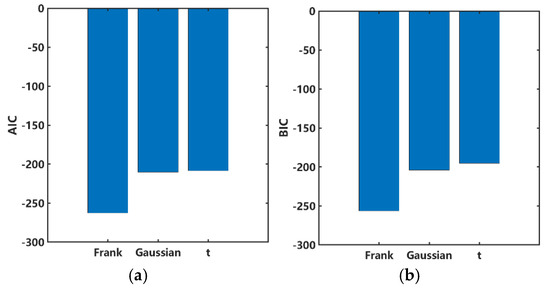
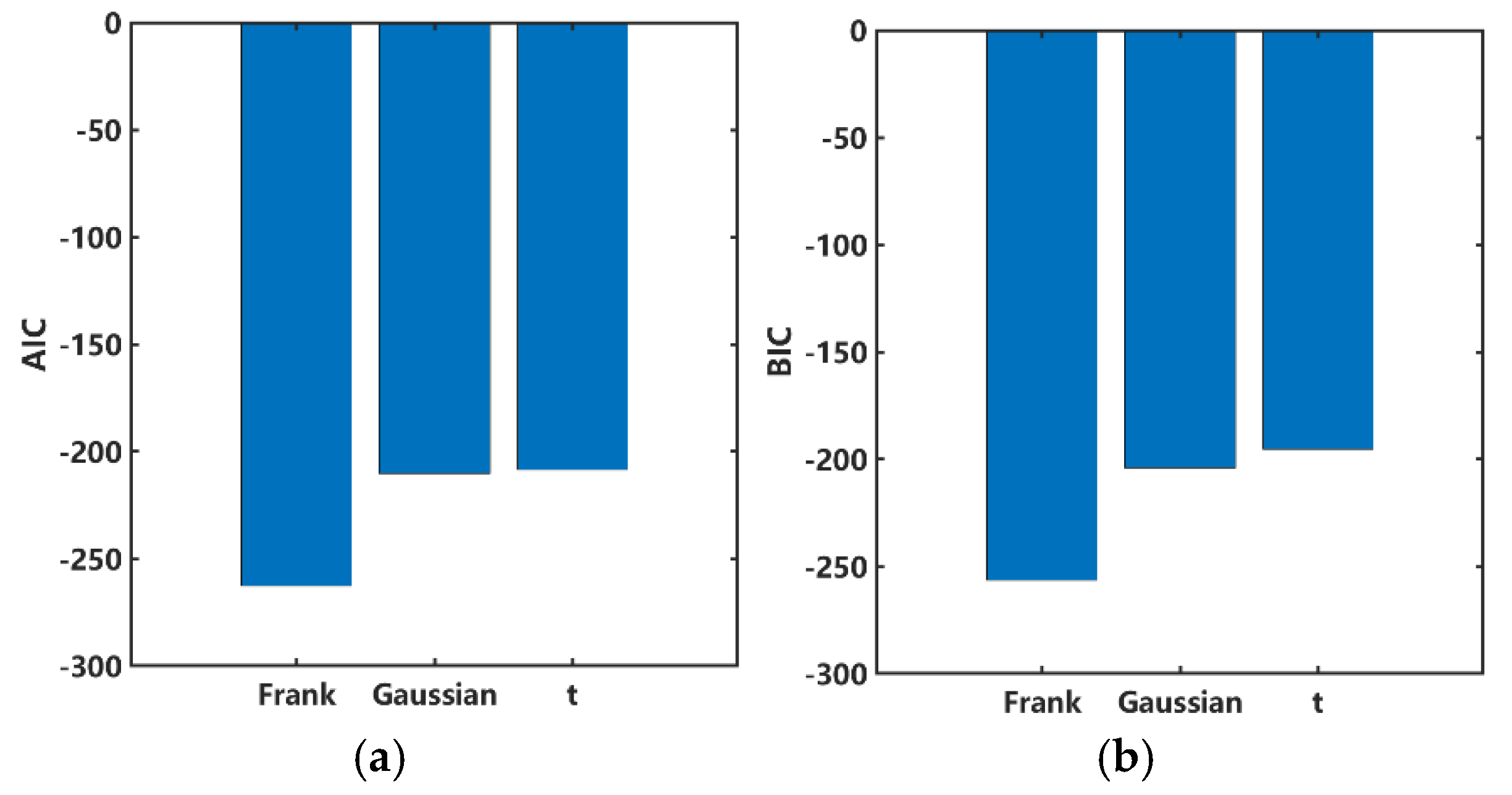
where $k$ denotes the number of model parameters, $L$ denotes the maximized likelihood value, and $n$ denotes the sample size. The results show a stable negative association between the cycle mean and cycle amplitude. The Pearson, Spearman, and Kendall correlation coefficients are −0.232838, −0.232838, and −0.150324, respectively, indicating that the two variables are not independent but exhibit moderate monotonic negative dependence. Further comparison of candidate Copula models reveals that the Frank Copula yields the highest log-likelihood value (132.390617). The AIC and BIC values—−262.781235 and −256.266244, respectively—are shown in Figure 10 and are superior to those of the Gaussian and Student’s t Copulas; the corresponding Frank parameter estimate is α = −1.375521. Therefore, the Frank Copula is selected as the optimal model for characterizing the joint distribution of the cycle mean and cycle amplitude.

Figure 10. Comparison of Copula model selection criteria: (a) AIC; (b) BIC.

5.2. Optimal Copula Model Verification

The distribution function of the optimal Frank Copula is:

$$C(u,v)=-{\displaystyle \frac{1}{\alpha }}\ln \left[1+{\displaystyle \frac{(e^{-\alpha u}-1)(e^{-\alpha v}-1)}{e^{-\alpha }-1}}\right]$$

(19)

Its probability density function is:

$$c(u,v)={\displaystyle \frac{\alpha (1-e^{-\alpha })e^{-\alpha (u+v)}}{{\left[(e^{-\alpha }-1)+(e^{-\alpha u}-1)(e^{-\alpha v}-1)\right]}^2}}$$

(20)

Furthermore, the joint density in the original variable space can be expressed as:

$$f_{X,Y}(x,y)=c(F_X(x),F_Y(y))f_X(x)f_Y(y)$$

(21)

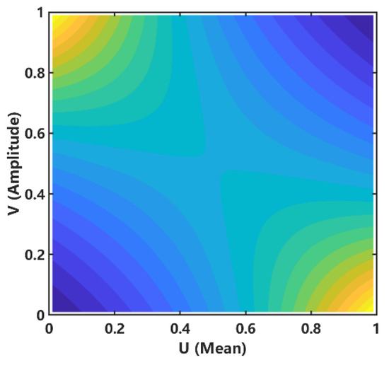
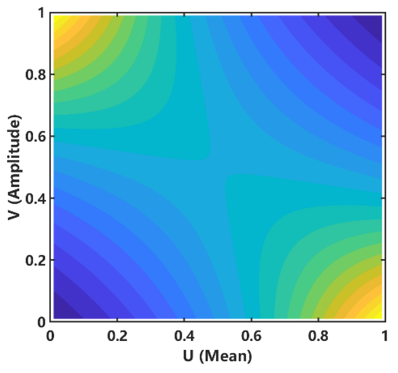
As shown in Figure 11, the joint density distribution of the optimal Frank Copula model reveals a well-defined negative association structure between the cycle mean and cycle amplitude. Moreover, this dependence structure exhibits no pronounced heavy-tailed behavior. Therefore, using the Frank Copula to characterize the coupling between the two variables is statistically well justified. Compared with linear correlation analysis—which captures only monotonic linear relationships—Copula modeling more effectively uncovers their joint variation patterns across the entire probability space while preserving the specified marginal distributions.

Figure 11. Joint density distribution of the fitted Frank Copula. The color gradient represents the magnitude of joint probability density, with warmer colors indicating higher density values.

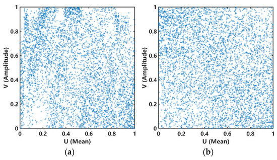
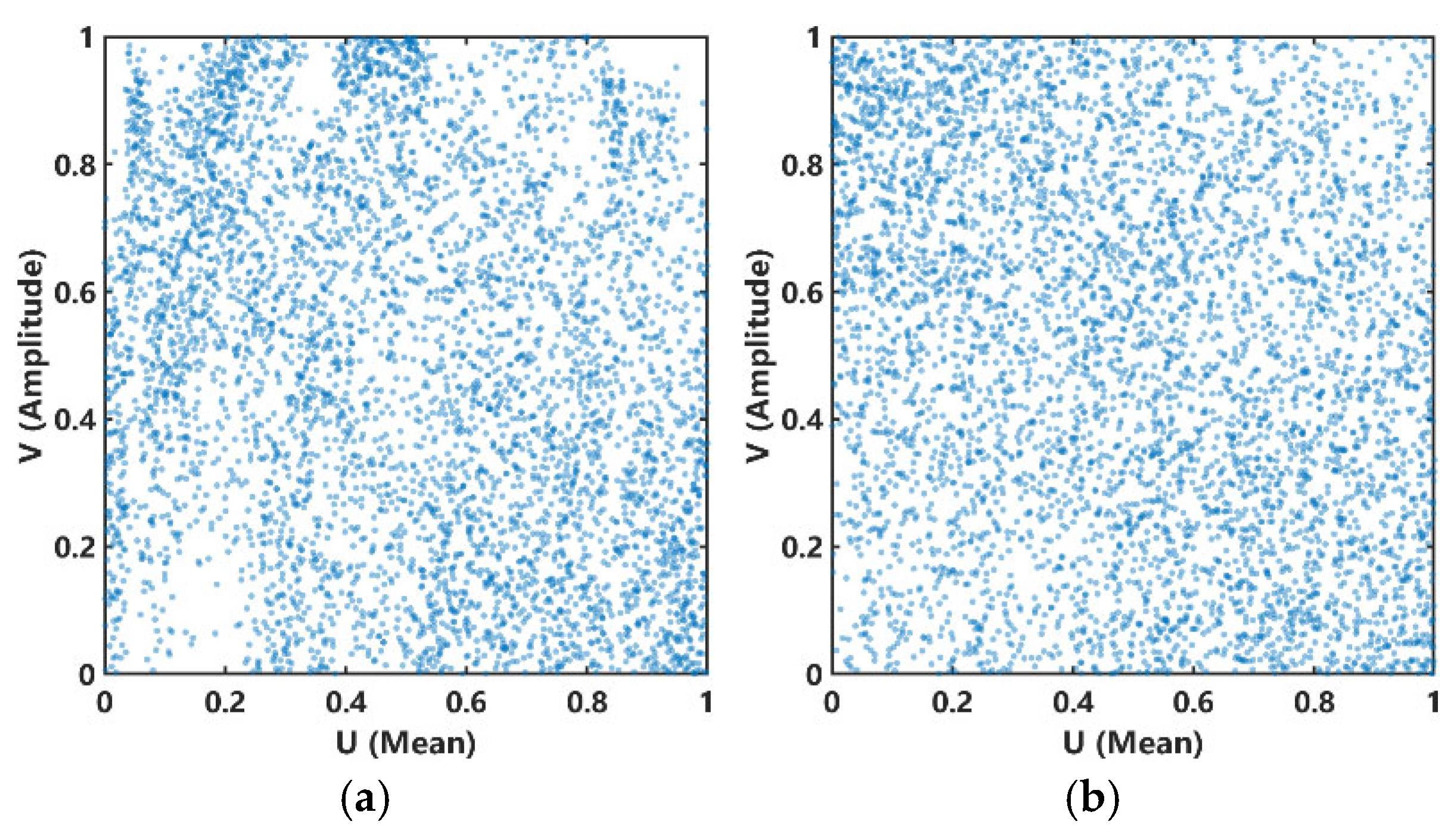
To further validate the ability of the optimal model to reproduce the sample-dependent dependence structure, pseudo-observations were simulated from the fitted Frank Copula—using the same sample size as the original data—and compared with the original pseudo-observations, as shown in Figure 12. The results show strong agreement between the simulated and original samples in terms of overall distribution range, scatter plot morphology, and monotonic negative association trend. This confirms that the model accurately reconstructs the joint distribution characteristics of the cycle mean and cycle amplitude. Quantitatively, the reproduction errors for Kendall’s τ and Spearman’s ρ are only 0.002964 and 0.013127, respectively, while the root-mean-square error (RMSE) of the empirical Copula surface is 0.007246—values that outperform all other candidate models. It should be noted that this model primarily captures the global dependence structure and has limited capacity to resolve local clustering or fine-scale discrete features present in the original samples. Nevertheless, this limitation does not compromise its suitability as the foundational model for subsequent random load spectrum reconstruction.

Figure 12. Comparison between the original and simulated pseudo-observations based on the Frank Copula: (a) original samples; (b) simulated samples.

5.3. Load Spectrum Reconstruction and Verification

After identifying the Frank Copula as the optimal model for characterizing the joint distribution of the cycle mean and cycle amplitude, this paper proceeds to reconstruct random load spectra. Based on the kernel density estimation (KDE)-derived marginal distributions and the fitted Frank Copula joint density function, two-dimensional probability integration over each load spectrum bin is performed to construct the reconstructed random load spectrum. Let the $i-th$ cycle mean bin and the $j-th$ cycle amplitude bin be $\left[m_i,m_{i+1}\right]$ and $\left[a_j,a_{j+1}\right]$, respectively; then the theoretical probability assigned to this bin is given by:

$$P_{ij}={\displaystyle {\int }_{m_i}^{m_i+1}{\displaystyle {\int }_{a_j}^{a_j+1}{f}_{M,A}(m,a)dadm}}$$

(22)

Combining the total number of cycles $N$, the theoretical frequency of the reconstructed load spectrum in the corresponding bin is given by:

$${\widehat{N}}_{ij}=N\cdot P_{ij}$$

(23)

To ensure that the reconstructed spectrum matches the statistical scale of the measured spectrum, this paper adopts the same binning scheme as the measured rainflow load spectrum: the cycle mean is discretized into 24 levels, and the cycle amplitude into 18 levels. Compared with frequency estimation via random sampling, this approach directly computes numerical integration over each bin using the joint probability density function—thereby effectively mitigating the impact of sampling variability from finite samples on the reconstructed spectrum matrix while preserving both marginal distribution consistency and dependence structure fidelity.

As shown in Table 1, the 24 × 18 reconstructed load spectrum—derived from the fitted Frank Copula joint density model—exhibits higher frequencies in the medium-to-high cycle mean and low-cycle-amplitude region. Overall, frequency declines with increasing amplitude, confirming that the reconstructed spectrum preserves the dominant distributional features of the measured rainflow load spectrum. To evaluate the effectiveness of the proposed model for random load spectrum reconstruction, this paper compares the reconstructed spectrum (based on the fitted Frank Copula joint density function) against the measured rainflow load spectrum and assesses reconstruction performance through two complementary metrics: marginal frequency distribution fidelity and error-based indicators.

Table 1. Reconstructed 24 × 18 torque load spectrum of the main shaft of the vertical ring-die biomass briquetting machine.

Cycle Mean	Cycle Amplitude
	0.1	0.2	0.3	0.4	0.5	0.6	0.7	0.8	0.9	1.0	1.2	1.3	1.4	1.5	1.6	1.7	1.8	2.0
437	4	4	5	5	6	5	5	4	3	3	2	2	1	1	1	0	0	0
438	5	6	7	7	8	8	7	5	4	3	3	2	2	1	1	1	0	0
440	6	7	8	9	9	9	8	6	5	4	3	3	2	1	1	1	0	0
441	7	8	9	10	11	10	9	7	6	5	4	3	2	2	1	1	1	0
442	7	8	9	10	11	10	9	7	6	4	3	3	2	2	1	1	0	0
443	9	11	12	13	13	12	11	9	7	5	4	3	3	2	1	1	1	0
445	10	12	13	14	14	13	12	9	7	6	4	4	3	2	1	1	1	0
446	10	12	13	14	14	13	11	9	7	5	4	3	3	2	1	1	1	0
447	11	13	14	14	15	14	12	9	7	6	4	3	3	2	1	1	1	0
448	13	14	15	16	16	15	13	10	8	6	4	4	3	2	1	1	1	0
449	19	21	23	23	24	21	18	14	11	8	6	5	4	3	2	1	1	1
451	30	32	34	34	34	30	25	19	15	11	9	7	5	4	3	2	1	1
452	35	38	39	38	37	33	27	20	16	12	9	7	5	4	3	2	1	1
453	39	41	41	40	38	33	26	19	15	11	8	7	5	4	3	2	1	1
454	46	47	46	43	40	34	27	19	15	11	8	7	5	4	2	2	1	1
455	60	59	56	52	47	39	30	21	16	12	9	7	5	4	3	2	1	1
457	71	68	62	56	49	39	30	21	16	12	9	7	5	4	2	2	1	1
458	71	65	58	50	43	34	25	18	13	10	7	5	4	3	2	1	1	1
459	61	54	47	39	33	25	19	13	10	7	5	4	3	2	1	1	1	0
460	49	42	35	29	24	18	13	9	7	5	3	3	2	1	1	1	0	0
462	49	42	34	28	23	17	12	8	6	4	3	2	2	1	1	1	0	0
463	41	33	27	22	17	13	9	6	5	3	2	2	1	1	1	0	0	0
464	25	21	16	13	10	8	5	4	3	2	1	1	1	1	0	0	0	0
465	13	10	8	6	5	4	3	2	1	1	1	1	0	0	0	0	0	0

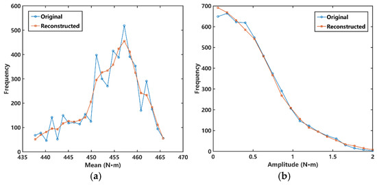
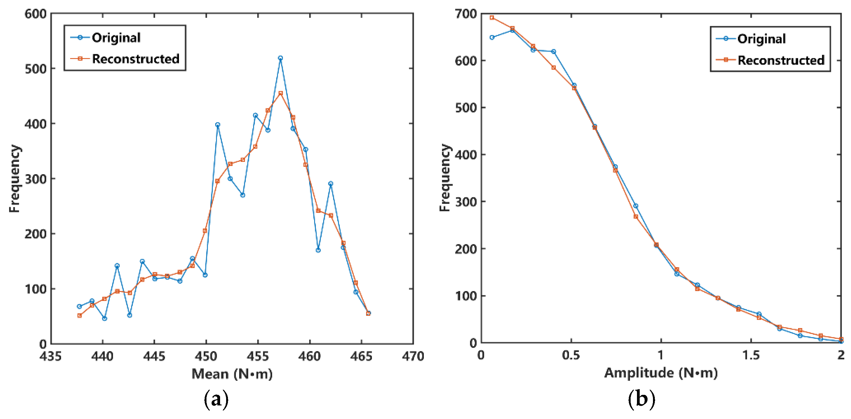
As shown in Figure 13, the comparison of marginal frequency distributions indicates that the reconstructed cycle amplitude marginal distribution is highly consistent with the measured one. The reconstructed spectrum captures the high-frequency concentration in the low-cycle-amplitude range and preserves the monotonic decreasing trend of frequency with increasing cycle amplitude. In contrast, although the reconstructed cycle mean marginal distribution shows minor discrepancies in local peak and trough locations, its primary operating range and dominant peak position remain well preserved. These results indicate that the Copula-based joint density integration method effectively captures the marginal statistical features and dominant peak-region distribution of the measured load spectrum.

Figure 13. Comparison of marginal frequency distributions between the measured and reconstructed load spectra: (a) cycle amplitude; (b) cycle mean.

To quantitatively evaluate the discrepancies between the reconstructed and measured load spectra, this paper adopts three error-based indicators: root-mean-square error (RMSE), normalized root-mean-square error (NRMSE), and relative error (RE). RMSE is used to measure the absolute frequency deviation between the reconstructed and measured load spectra. Because RMSE depends on the frequency scale of the load spectrum, NRMSE and RE are further introduced to provide a normalized evaluation of the reconstruction accuracy. The RMSE is expressed as:

$$RMSE=\sqrt{{\displaystyle \frac{1}{rs}}{\displaystyle \sum _{i=1}^r{\displaystyle \sum _{j=1}^s{({\widehat{N}}_{ij}-N_{ij})}^2}}}$$

(24)

$$NRMSE={\displaystyle \frac{RMSE}{n_{\max }-n_{\min }}}\times 100\%$$

(25)

$$RE={\displaystyle \frac{{\displaystyle \sum _{i=1}^r{\displaystyle \sum _{j=1}^s\left|n_{ij}-{\widehat{n}}_{ij}\right|}}}{{\displaystyle \sum _{i=1}^r{\displaystyle \sum _{j=1}^s{n}_{ij}}}}}\times 100\%$$

(26)

where $r$ and $s$ denote the number of bins for the cycle mean and cycle amplitude, respectively; ${\mathrm{n}}_{ij}$ and ${\widehat{n}}_{ij}$ denote the measured and reconstructed frequencies in the $i-th$ mean bin and $j-th$ amplitude bin, respectively; $n_{\max }$ and $n_{\min }$ are the maximum and minimum frequencies in the measured load spectrum. The relative error evaluates the total absolute deviation between the reconstructed and measured spectra relative to the total number of measured cycles, which avoids the instability caused by zero-frequency bins in sparse two-dimensional load spectrum matrices.

To further evaluate whether the obtained RMSE value indicates acceptable reconstruction performance, a KDE-independent baseline model was constructed for comparison. In this baseline model, the marginal distributions of the cycle mean and cycle amplitude were estimated using KDE in the same way as in the proposed model, but the dependence structure between the two variables was ignored. Therefore, the joint probability density was approximated as the product of the two marginal densities:

$${\widehat{f}}_{\mathrm{ind}}(m,a)={\widehat{f}}_M(m){\widehat{f}}_A(a)$$

(27)

As shown in Table 2, the proposed KDE–Frank Copula model achieves lower RMSE, NRMSE, and relative error than the KDE-independent baseline model. Compared with the baseline model, the RMSE is reduced from 7.2387 to 6.3161, corresponding to an improvement of 12.74%. Meanwhile, the relative error decreases from 41.53% to 36.56%, corresponding to an improvement of 11.97%. These results indicate that the dependence structure between the cycle mean and cycle amplitude cannot be ignored. By introducing the Frank Copula function, the proposed model better preserves the joint statistical characteristics of the measured torque load and improves the reconstruction accuracy of the random load spectrum.

Table 2. Error comparison between the KDE-independent baseline model and the proposed KDE–Frank Copula model.

Model	Dependence Structure	RMSE	NRMSE (%)	Relative Error (%)
KDE-independent baseline model	Independence assumption	7.2387	7.9546	41.5314
Proposed KDE–Frank Copula model	Frank Copula dependence	6.3161	6.9408	36.5604

It should be noted that the reconstructed load spectrum exhibits residual deviations in reproducing local peak frequencies and fine-scale discrete features. This arises because the joint density integration method prioritizes smooth reconstruction of the global statistical structure, whereas its capacity to resolve local clusters and irregular fluctuations present in the original samples remains limited. Consequently, this method is better suited for overall statistical reconstruction and engineering-level characterization of random load spectra—not for pixel-accurate gridded reproduction. Nevertheless, as evidenced by the marginal distribution trend agreement and dominant peak interval alignment, the proposed method faithfully preserves the joint statistical characteristics of the cycle mean and cycle amplitude, thereby providing foundational data and methodological support for subsequent fatigue load characterization, life prediction, and reliability analysis.

From an engineering application perspective, the reconstructed load spectrum can help identify the dominant operating load range and the high-amplitude load cycles that are potentially more damaging to the main shaft. Therefore, the results can support operating parameter optimization, stable feeding control, and structural reliability-oriented design, thereby reducing torque fluctuation, improving operating stability, and extending the service life of the vertical ring-die biomass briquetting machine.

6. Conclusions

(1)

The measured main shaft torque signal was processed using wavelet-threshold denoising and four-point rainflow counting to extract cycle mean and cycle amplitude features. The cycle mean is mainly concentrated around 455 N·m, while the cycle amplitude is primarily distributed within 0–1.0 N·m. Independence testing and correlation analysis confirm a statistically significant dependence between the cycle mean and cycle amplitude, indicating that they should not be treated as independent random variables.

(2)

KDE was used to model the marginal distributions of the cycle mean and cycle amplitude, and a Copula-based joint distribution model was constructed. Model selection results show that the Frank Copula provides the best description of the dependence structure between the two variables.

(3)

A random load spectrum reconstruction method was developed based on the KDE-derived marginal distributions and the fitted Frank Copula joint density model. The reconstructed spectrum agrees well with the measured spectrum in terms of cycle amplitude marginal distribution, dominant cycle mean range, and main peak-region location. The RMSE and NRMSE are 6.3161 and 6.94%, respectively. Compared with the KDE-independent baseline model, the proposed KDE–Frank Copula model reduces the RMSE by 12.74%, demonstrating that the dependence structure improves the reconstruction accuracy. This method provides support for load spectrum generation, fatigue life prediction, reliability analysis, and structural optimization of vertical ring-die biomass briquetting machines. The reconstructed load spectrum can serve as a quantitative load input for subsequent fatigue damage calculation and reliability-oriented structural design of the main shaft.

References

- Yang, P.; Zhang, S.N.; Zhong, Z.; Wang, H.; Liu, H.; Wang, Y.; Wang, K. Fuel molding of cattle manure mixed with biomass pellet and its characteristic analysis. J. Agric. Resour. Environ. 2022, 39, 586–593. [Google Scholar]
- Vaish, S.; Sharma, N.K.; Kaur, G. A review on various types of densification/briquetting technologies of biomass residues. IOP Conf. Ser. Mater. Sci. Eng. 2022, 1228, 012019. [Google Scholar] [CrossRef] [Scilit]
- Brunerová, A.; Brožek, M.; Van Dung, D.; Phung, L.D.; Hasanudin, U.; Iryani, D.A.; Chaloupková, V.; Roubík, H. Manual wooden low-pressure briquetting press: An alternative technology of waste biomass utilisation in developing countries of Southeast Asia. J. Clean. Prod. 2024, 436, 140624. [Google Scholar] [CrossRef] [Scilit]
- Wang, Z.; Quan, Z.Q.; He, H. Predicting model for fatigue life of mechanical structures under random cyclic loads. China Mech. Eng. 2012, 23, 98–101. [Google Scholar]
- Wu, Q.; Zhao, Y.; Liu, X. Fatigue life prediction of metal materials under random loads based on load spectrum extrapolation. Int. J. Fatigue 2024, 187, 108473. [Google Scholar] [CrossRef] [Scilit]
- Wei, G.Q.; He, W.B.; Yan, M.Y.; Zhao, G. Load spectrum design and experimental verification of nonlinear damage model. Res. Explor. Lab. 2023, 42, 1–6. [Google Scholar]
- Yin, X.K.; Fang, F.; Li, J.S.; Zhao, W.H. Compilation of test load spectrum for main bearing of robot RV reducer. Modul. Mach. Tool Autom. Manuf. Tech. 2023, 2, 121–124. [Google Scholar]
- Du, J.; Hai, X.H.; He, Y.L.; Lv, X.F. Fatigue analysis on main shaft in MW level wind turbine. Acta Energiae Solaris Sin. 2013, 34, 591–597. [Google Scholar]
- Mai, Z.H.; Peng, Z.Z.; Tian, C.Q.; Wan, Z.P. Load spectrum construction of a jack-up offshore platform lifting system. J. Mech. Transm. 2025, 49, 170–176. [Google Scholar]
- Hu, B.; Li, Y.; Yang, H.; Wang, H. Wind speed model based on kernel density estimation and its application in reliability assessment of generating systems. J. Mod. Power Syst. Clean Energy 2017, 5, 220–227. [Google Scholar]
- Duda, P.; Rutkowski, L.; Jaworski, M.; Rutkowska, D. On the Parzen kernel-based probability density function learning procedures over time-varying streaming data with applications to pattern classification. IEEE Trans. Cybern. 2020, 50, 1683–1696. [Google Scholar] [PubMed]
- Sidibé, I.; Khatab, A.; Diallo, C.; Adjallah, K. Kernel estimator of maintenance optimization model for a stochastically degrading system under different operating environments. Reliab. Eng. Syst. Saf. 2016, 147, 109–116. [Google Scholar] [CrossRef] [Scilit]
- Wang, P.; Deng, H.; Wang, Y.M.; Liu, Y.; Zhang, Y. Kernel density estimation based Gaussian and non-Gaussian random vibration data induction for high-speed train equipment. IEEE Access 2020, 8, 90914–90923. [Google Scholar] [CrossRef] [Scilit]
- Wang, D.; Li, M. Robust stochastic configuration networks with kernel density estimation for uncertain data regression. Inf. Sci. 2017, 412–413, 210–222. [Google Scholar] [CrossRef] [Scilit]
- Zhang, L.; Lin, J.; Karim, R. Adaptive kernel density-based anomaly detection for nonlinear systems. Knowl. Based Syst. 2018, 139, 50–63. [Google Scholar] [CrossRef] [Scilit]
- Xu, Y.Q.; Chen, K.; Li, J.Q.; Nie, Y. A new method analyzing output correlation of multi-wind farms based on combination of Copula function and kernel estimation theory. Trans. China Electrotech. Soc. 2016, 31, 92–100. [Google Scholar]
- Wang, Q. System Reliability Analysis and Risk Priority Number Calculation Method Based on Copula Function. Master’s Thesis, University of Electronic Science and Technology of China, Chengdu, China, 2021. [Google Scholar]
- Zi, J.J.; Zhang, T.; Wang, Y. Reliability assessment of electric spindle based on performance degradation model of Copula function. Mach. Tool Hydraul. 2025, 53, 58–62. [Google Scholar]
- Bao, D.; Gao, F.; Wang, P.; Zhang, S.; Han, F. Research and forecasting analysis of blade load correlation based on Copula function. Acta Energiae Solaris Sin. 2023, 44, 323–329. [Google Scholar]
- Cui, L.M.; Ma, Z.Y.; Chen, X.; Liu, Y.F.; Zhang, H. Wind-PV-Load joint scene generation method based on kernel density estimation and Copula function. Coal Econ. Res. 2026, 46, 153–161. [Google Scholar]
- Gao, Y.J.; Yang, Y.F.; Chen, J.; Yang, C.Y. A research on load spectrum statistical analysis of T100C train bogie based on kernel density estimation algorithm. J. Mech. Strength 2016, 38, 1330–1334. [Google Scholar]
- Li, C.P.; Wang, Y.L.; Zhu, X.X.; Qi, X.; Guan, X.; Li, J.; Chang, Z.; Bai, Y.; Li, H. Copula function based on second-order cone relaxation optimal power flow and robust weighted K-means method for PV carrying capacity evaluation. Adv. Technol. Electr. Eng. Energy 2025, 44, 74–88. [Google Scholar]
- Pan, X.; Wang, L.L.; Xu, Y.Q.; Zhang, L.; Liu, W.; Wu, R. A wind farm power modeling method based on mixed Copula. Autom. Electr. Power Syst. 2014, 38, 17–22. [Google Scholar]
- Wang, S.Y.; Liang, R.L.; Wu, Z.; Gao, F.L.; Wu, Y. Extrapolation of stack load spectrum for fuel cell bus based on kernel density estimation. J. Highw. Transp. Res. Dev. 2026, 43, 223–230. [Google Scholar]
- Liu, H.; Xu, H.X. Research on compiling method of crane stress spectrum based on kernel density estimation. Hoisting Conveying Mach. 2024, 9, 56–61. [Google Scholar]
- He, X.Y.; Xiao, F.X.; Yang, Q.; Zhang, Y.W.; Chen, J.Y. Stress spectrum extrapolation and fatigue life analysis of frame based on kernel density estimation. Hoisting Conveying Mach. 2023, 1, 51–56. [Google Scholar]
- Lan, L.F. Compiling Load Spectrum of Machining Center Spindle by the Diffusion-Based Kernel Method. Master’s Thesis, Jilin University, Changchun, China, 2022. [Google Scholar]
Disclaimer/Publisher’s Note: The statements, opinions and data contained in all publications are solely those of the individual author(s) and contributor(s) and not of MDPI and/or the editor(s). MDPI and/or the editor(s) disclaim responsibility for any injury to people or property resulting from any ideas, methods, instructions or products referred to in the content. |
© 2026 by the authors. Licensee MDPI, Basel, Switzerland. This article is an open access article distributed under the terms and conditions of the Creative Commons Attribution (CC BY) license.