Analysis on the Compensation Efficacy of Gravity Field Spherical Harmonic Models of Different Degrees for High-Precision Inertial Navigation Systems

Abstract

In long-endurance and high-precision navigation scenarios, gravity disturbances have become the core bottleneck limiting the performance improvement of high-precision Inertial Navigation Systems (INSs). This paper aims to investigate the compensation efficacy of gravity field spherical harmonic models of different degrees for high-precision INS. The influence mechanisms of gravity disturbances on INS error propagation are derived, and corresponding simulation analyses are performed. The gravity compensation mechanism based on gravity field spherical harmonic models is elaborated, and the performance differences in gravity disturbance compensation among spherical harmonic models of different orders are comparatively analyzed. Based on long-endurance ship trial experiments using high-precision inertial navigation equipment, the compensation efficacy of the 360-order and 2159-order compensation schemes on multiple navigation performance indicators is quantitatively evaluated across sea areas with different gravity characteristics. The experimental results demonstrate that the widely held consensus within the field—that a higher model degree yields better compensation efficacy when improving high-precision INS accuracy based on gravity field spherical harmonic model compensation—does not hold universal applicability. The research findings can provide theoretical support for the engineering implementation of gravity compensation schemes and the selection of model degrees for high-precision INS.

1. Introduction

Inertial navigation is an autonomous navigation technology. By utilizing gyroscopes to measure the carrier’s angular velocity and accelerometers to measure its linear acceleration, it integrates the measured angular velocity and acceleration to calculate the carrier’s current position, velocity, and attitude parameters in real time. It features the advantages of strong autonomy, excellent concealment, and high short-term accuracy. However, during the long-term operation of the system, the measurement errors of the inertial components will continuously accumulate through integration, leading to the divergence of navigation errors. For the INS, since the navigation calculation and output highly depend on the absolute acceleration vector, and the measurement of absolute motion acceleration is deeply coupled with the Earth’s gravity vector, the accuracy of gravity information plays a crucial role in both the initial alignment and dead reckoning of the system [1].

In recent years, with rapid breakthroughs in the manufacturing processes of core sensors such as high-precision optical gyroscopes, the inherent hardware errors of high-precision INS have been significantly reduced. To further break through the physical accuracy limits of these devices, system-level error suppression technologies such as rotation modulation have been widely applied [2,3,4]. This technology drives the Inertial Measurement Unit (IMU) to undergo periodic rotations via a high-precision turntable, effectively canceling out the constant drift and bias of the sensors during navigation calculations. However, the extreme compression of internal hardware errors makes the system highly sensitive to the objective interference of external physical fields. For low-precision INS, the primary errors are system errors; thus, gravity disturbance errors are comparatively negligible, and adopting a normal gravity model on the Earth’s reference ellipsoid is usually sufficient to meet the requirements. But for modern INS with extremely high precision and error suppression technologies, system hardware errors become secondary, and the impact of external gravity disturbances becomes increasingly prominent. This is especially true for horizontal gravity disturbances [5], which can reach hundreds of milligals (mGal) in regions with undulating terrain or dramatic variations in the gravity field [6].

Gravity disturbances have a positive correlation with INS errors; that is, the larger the amplitude of the gravity disturbance, the larger the error generated by the INS. In high-precision INS, the errors induced by gravity disturbances are among the main error sources restricting navigation accuracy [7]. These errors continuously accumulate as navigation time increases, and their impact is particularly pronounced in long-endurance application scenarios. Therefore, high-precision INS can no longer simply use normal gravity to replace actual gravity; the effects of gravity disturbances must be fully considered, and targeted research on gravity field compensation must be conducted. Taking gravity disturbance as the core research object, this paper systematically elaborates on the action mechanism of gravity disturbances on the INS and uses simulation to analyze their influence laws on navigation calculation accuracy. Meanwhile, combined with verification from actual ship trials, it comparatively analyzes the compensation effects of gravity field spherical harmonic models of varying degrees on the impact of gravity disturbances within the INS.

2. Influence Mechanism and Simulation Analysis of Gravity Disturbance on INS

2.1. Analysis of Gravity Disturbance Influence Mechanism

In the local geographic coordinate system ($n$-frame, where the East-North-Up coordinate system is selected in this paper), the specific force equation of the INS can be expressed as:

$${\dot{v}}^n=C_b^n{f}^b-\left(2{\omega }_{ie}^n+{\omega }_{en}^n\right)\times v^n+g^n$$

(1)

where ${\mathit{v}}^{\mathit{n}}$ is the velocity vector of the carrier in the $n$-frame; $C_b^n$ is the attitude direction cosine matrix from the body coordinate system ($b$-frame) to the $n$-frame; ${\mathit{f}}^{\mathit{b}}$ is the specific force vector output by the accelerometer; ${\mathit{\omega }}_{\mathit{ie}}^{\mathit{n}}$ and ${\mathit{\omega }}_{\mathit{en}}^{\mathit{n}}$ are the projection vectors of the Earth’s rotation angular velocity and the carrier’s motion angular velocity in the $n$-frame, respectively; ${\mathit{g}}^{\mathit{n}}$ is the true Earth gravity vector at the carrier’s location.

In traditional INS calculations, the normal gravity model ${\mathit{\gamma }}^{\mathit{n}}$ on the reference ellipsoid is usually adopted to approximate the true gravity [8]. However, due to the uneven distribution of mass within the Earth and the undulations of the surface terrain, an objective difference exists between the true gravity vector and the normal gravity vector, and this difference is the gravity disturbance vector $\mathit{\delta }{\mathit{g}}^{\mathit{n}}$:

$$\mathit{\delta }{\mathit{g}}^{\mathit{n}}={\mathit{g}}^{\mathit{n}}-{\mathit{\gamma }}^{\mathit{n}}$$

(2)

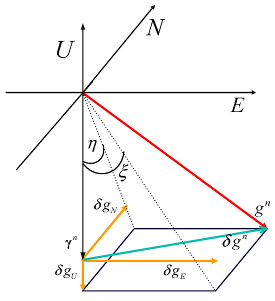
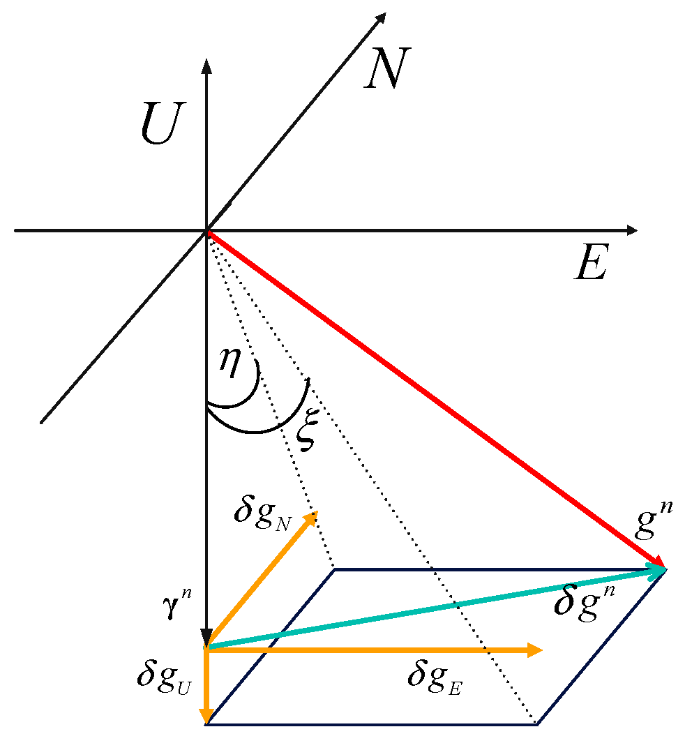
In the local geographic coordinate system, the gravity disturbance vector $\mathit{\delta }{\mathit{g}}^{\mathit{n}}$ can be decomposed into three components: East, North, and Up. Among them, the horizontal gravity disturbance is primarily manifested as a deflection in the direction of the gravity vector, namely the deflection of the vertical; the Up component is manifested as an anomaly in magnitude, namely the gravity anomaly. The projection of the gravity disturbance in the $n$-frame can be expressed as [7]:

$$\mathit{\delta }{\mathit{g}}^{\mathit{n}}=\left[\begin{array}{c}\delta g_E\\ \delta g_N\\ \delta g_U\end{array}\right]\approx \left[\begin{array}{c}-g\eta \\ -g\xi \\ \Delta g\end{array}\right]$$

(3)

To intuitively describe the physical significance and component structure of the gravity disturbance, a schematic diagram of the gravity disturbance in the local geographic coordinate system is provided, as shown in Figure 1. The horizontal gravity disturbance components $\delta g_E$ and $\delta g_N$ are converted from the deflection of the vertical $\eta$ and $\xi$, while the vertical component $\delta g_U$ corresponds to the gravity anomaly $\Delta g$. All components typically range from tens to hundreds of milligals, falling within the same order of magnitude, yet they characterize different physical features of the anomalous gravity field.

Figure 1. Schematic diagram of gravity disturbance.

By performing a micro-perturbation analysis on the ideal specific force equation, the system velocity error state equation containing the gravity disturbance can be obtained [9]:

$$\mathit{\delta }{\dot{\mathit{v}}}^{\mathit{n}}={\mathit{f}}^{\mathit{n}}\times \mathit{\varphi }+C_b^n\mathit{\delta }{\mathit{f}}^{\mathit{b}}-\left(2{\mathit{\omega }}_{\mathit{ie}}^{\mathit{n}}+{\mathit{\omega }}_{\mathit{en}}^{\mathit{n}}\right)\times \mathit{\delta }{\mathit{v}}^{\mathit{n}}-\left(2\mathit{\delta }{\mathit{\omega }}_{\mathit{ie}}^{\mathit{n}}+\mathit{\delta }{\mathit{\omega }}_{\mathit{en}}^{\mathit{n}}\right)\times {\mathit{v}}^{\mathit{n}}+\mathit{\delta }{\mathit{g}}^{\mathit{n}}$$

(4)

where $\mathit{\varphi }$ is the attitude error angle vector; $\mathit{\delta }{\mathit{f}}^{\mathit{b}}$ is the accelerometer measurement error. In this equation, the gravity disturbance term $\mathit{\delta }{\mathit{g}}^{\mathit{n}}$ and the accelerometer’s own measurement error $C_b^n\mathit{\delta }{\mathit{f}}^{\mathit{b}}$ are mathematically equivalent, constituting error driving sources of the same magnitude. Especially in rotation-modulated inertial navigation systems, the constant error of the accelerometer rigidly attached to the body coordinate system is periodically counteracted within a single rotation cycle. As a result, $\mathit{\delta }{\mathit{f}}^{\mathit{b}}$ is effectively suppressed and tends to zero, and the externally introduced gravity disturbance $\mathit{\delta }{\mathit{g}}^{\mathit{n}}$ naturally becomes the dominant excitation term leading to navigation error divergence. Uncompensated horizontal gravity disturbances will directly enter the integration loop as horizontal acceleration error terms in the navigation coordinate system, exciting Schuler oscillations with a period of approximately 84.4 min [10,11].

2.2. Simulation Analysis of the Impact of Gravity Disturbance on System Accuracy

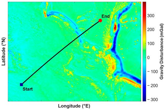
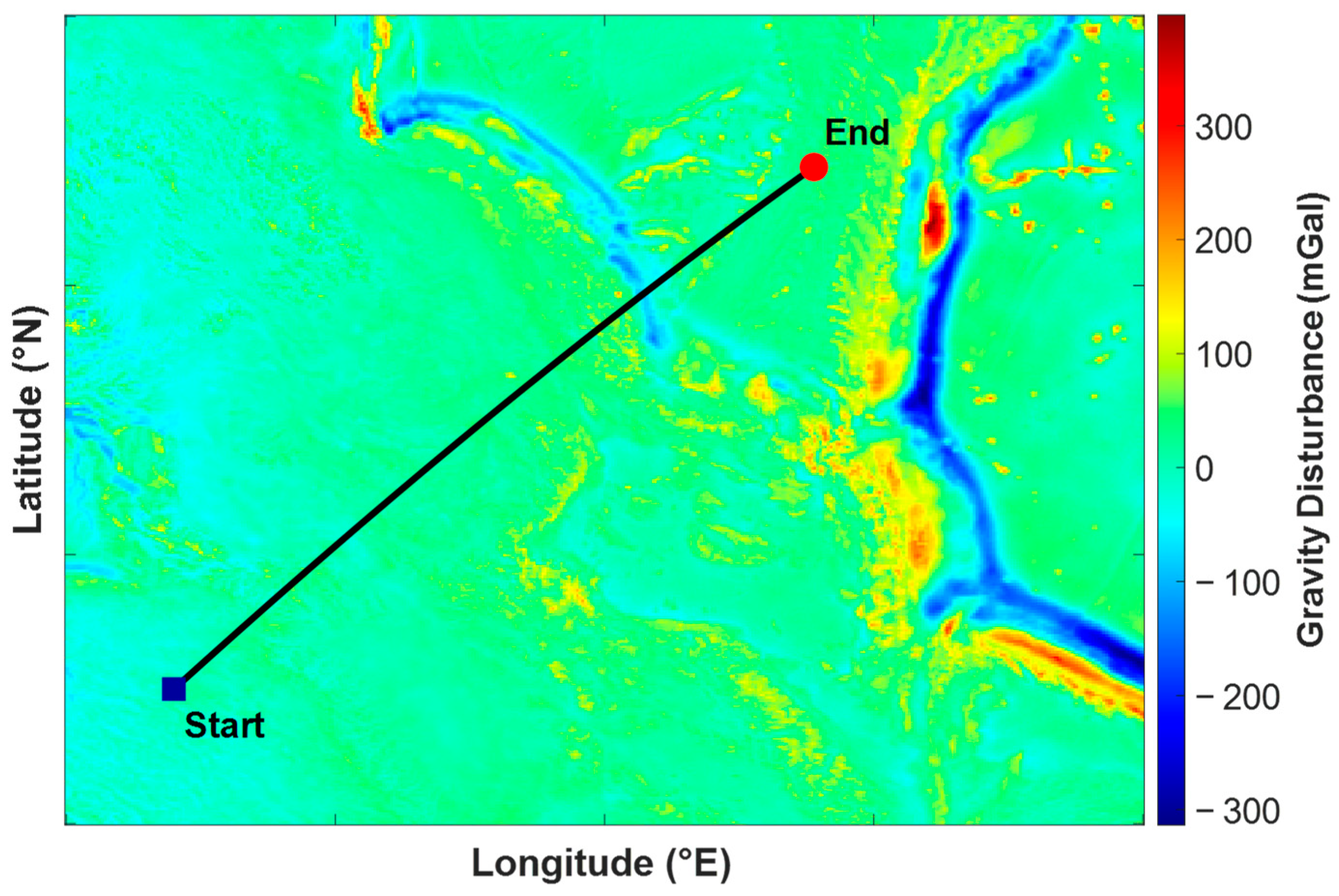
This section quantitatively evaluates the impact of gravity disturbances on the performance indicators of high-precision INS through simulation experiments. The simulation assumes that the carrier is located near the ground at a latitude of 25° N ($h=0$), navigating at a constant speed of 10 m/s with a heading angle of 45° (with equal East and North velocity components), while other attitude angles (pitch and roll) are assumed to be zero and remain unchanged throughout the simulation. The total simulation time is set to $60 \mathrm{h}$. To isolate other error sources, the simulation does not consider the measurement errors of the gyroscopes and accelerometers, sets the initial state errors to zero, and approximates the radii of the Earth’s meridian and prime vertical circles as the Earth’s average radius (approximately 6,371,000 m). Corresponding simulated trajectory and gravity disturbance field distribution are shown in Figure 2.

Figure 2. Simulation trajectory and corresponding regional gravity disturbance field.

According to the statistics of the 2159th-degree coefficients of the EGM2008 gravity field model, the root mean square (RMS) value of global horizontal gravity disturbances is approximately 32.7 mGal. Considering that the altitude channel of a high-precision INS is usually in a damped state, the impact of vertical gravity disturbances on the overall navigation accuracy of the system is relatively small [12]. Therefore, this experiment focuses on horizontal gravity disturbances, injecting a gravity disturbance of 32.7 mGal into the East and North directions, respectively, as the basic calculation. To comprehensively evaluate the system’s sensitivity to gravity interference of different intensities, the experiment further sets up various operating conditions, such as constant and random gravity disturbances, and separately analyzes the East-North-Up attitude errors ${\varphi }_{E/N/U}$, the East-North velocity errors $\delta v_{E/N}$, and the radial position error $\delta S$. The relevant simulation comparison results are shown in Table 1.

Table 1. INS Errors Induced by Horizontal Gravity Disturbances.

No.	Disturbance Condition	${\mathit{\varphi }}_{\mathit{E}} {(}^{″})$	${\mathit{\varphi }}_{\mathit{N}} {(}^{″})$	${\mathit{\varphi }}_{\mathit{U}} {(}^{″})$	$\mathit{\delta }{\mathit{v}}_{\mathit{E}} (\mathbf{k}\mathbf{n})$	$\mathit{\delta }{\mathit{v}}_{\mathit{N}} (\mathbf{k}\mathbf{n})$	$\mathit{\delta }\mathit{S} (\mathbf{nmile})$
1	East $32.7 \mathrm{mGal}$ + North $32.7 \mathrm{mGal}$	14.4	14.4	7.2	0.58	0.58	0.38
2	East $50 \mathrm{mGal}$	5.4	10.8	7.2	0.09	0.01	0.32
3	North $50 \mathrm{mGal}$	10.8	5.4	7.8	0.01	0.12	0.30
4	East $100 \mathrm{mGal}$	21	32.4	19.8	0.96	0.90	0.69
5	North $100 \mathrm{mGal}$	9	34.2	24.6	1.17	1.14	0.70
6	Horizontal Random $32.7 \mathrm{mGal}$	5.4	5.4	2.9	0.39	0.29	0.11
7	East $50 \mathrm{mGal}+50\sin ({\omega }_{ie}T) \mathrm{mGal}$	19.2	31.2	19.8	0.96	0.89	0.69
8	East $100 \mathrm{mGal}+100\sin ({\omega }_{ie}T) \mathrm{mGal}$	66	83.4	51.6	4.05	3.96	1.4
9	North $30 \mathrm{mGal}+30\sin ({\omega }_{ie}T) \mathrm{mGal}$	16.2	8.4	0	0.02	0.17	0.70
10	North $50 \mathrm{mGal}+50\sin ({\omega }_{ie}T) \mathrm{mGal}$	32.4	22.2	9	1.17	1.15	0.70

Among these, the horizontal random gravity disturbance consists of East and North components, and its temporal variation follows the standard continuous first-order Gauss–Markov model:

$$\dot{\eta }(t)=-{\displaystyle \frac{1}{\beta }}\eta (t)+\sqrt{{\displaystyle \frac{2{\sigma }^2}{\beta }}}w(t)$$

(5)

The first-order Markov model is widely adopted to characterize the temporal correlation of gravity disturbances, which have prominent autocorrelation over short and medium time spans. In the formula, $\beta$ denotes the correlation time constant of the stochastic process with the unit of second, and we set $\beta = 15 \mathrm{s}$ in this work. $w(t)$ represents continuous Gaussian white noise. The parameter σ directly stands for the steady-state root-mean-square of horizontal gravity disturbance, which is exactly the 32.7 mGal listed in Table 1. This value is obtained from statistical calculation of global horizontal gravity disturbances using the 2159th-degree spherical harmonic coefficients of the EGM2008 gravity field model.

By conducting a comparative analysis of the quantified data in Table 1, the following conclusions can be drawn:

• The total values of position errors, velocity errors, and attitude errors caused by horizontal gravity disturbances are basically the same; only the projection directions of the velocity errors and attitude errors differ.
• The influence of horizontal gravity disturbances on navigation accuracy mainly depends on their combined magnitude. Even if the gravity disturbance component in a single direction is small, as long as the combined magnitude is large, it will still have a significant impact on navigation accuracy.

3. Compensation Technology and Degree Characteristics Analysis Based on Gravity Field Spherical Harmonic Model

The compensation method based on the gravity field spherical harmonic model essentially expands the Earth’s true disturbing gravity potential into a spatially linear combination of a series of spherical harmonic functions. In current engineering applications, the EGM2008 model released by the National Geospatial-Intelligence Agency (NGA) of the United States is the most typical example [13]. At a given spatial position (geocentric radius $r$, geocentric colatitude $\theta$, longitude $\lambda$), the spherical harmonic expansion of the Earth’s disturbing gravity potential $T$ can be strictly expressed as [14]:

$$T(r,\theta ,\lambda )={\displaystyle \frac{GM}{r}}{\displaystyle {\displaystyle \sum _{n=2}^{N_{max}}}{\left(\frac{a}{r}\right)}^n}{\displaystyle {\displaystyle \sum _{m=0}^n}\left[\Delta {\overline{C}}_{nm}\cos m\lambda +\Delta {\overline{S}}_{nm}\sin m\lambda \right]}{\overline{P}}_{nm}(\cos \theta )$$

(6)

In the formula, $GM$ is the Earth’s gravitational constant; $a$ is the semi-major axis of the reference ellipsoid; $N_{max}$ is the highest truncation degree of the model; $n$ and $m$ are the degree and order of the spherical harmonic expansion, respectively; $\Delta {\overline{C}}_{nm}$ and $\Delta {\overline{S}}_{nm}$ are the fully normalized disturbing potential coefficients; and ${\overline{P}}_{nm}(\cos \theta )$ is the fully normalized associated Legendre function. By taking spatial partial derivatives of the disturbing gravity potential $T$ in the north, east, and up directions of the local geographic coordinate system, the vertical deflection and gravity anomaly at the current position can be analytically calculated.

In the selection of the truncation degree $N_{max}$ for the spherical harmonic compensation model of the gravity field, it represents a core theoretical parameter that determines the trade-off between compensation accuracy and system computational burden. From the perspective of spatial frequency domain analysis, the spherical harmonic function, through truncation at degree $N_{max}$, divides the Earth’s surface into alternating grid regions in the latitude and longitude directions. The actual geographic half-wavelength corresponding to adjacent zero lines is defined as the spatial resolution $D$ of the gravity field model [15]. The magnitude of the spatial resolution directly determines the gravity field model’s capability to capture fine details of local gravity disturbances in the real world: high-resolution models can accurately depict high-frequency short-wavelength anomalies that easily excite system comfort oscillations, whereas low-resolution models can only reflect the smooth long-wavelength macroscopic features. In actual engineering calculations, the spatial resolution $D$ is typically represented intuitively by the surface distance (in kilometers). There exists a strict inverse proportional mathematical relationship between the truncation degree $N_{max}$ of the spherical harmonic model and its corresponding terrestrial spatial resolution [16], as shown in the following formula:

$$D={\displaystyle \frac{\pi R_e}{N_{max}}}$$

(7)

In the formula, $R_e$ is the Earth’s mean radius (approximately 6371 km). In engineering estimations, this spatial resolution is often simplified to $D\approx \mathrm{20,000}/N_{max} \left(\mathrm{km}\right)$.

For high-precision inertial navigation systems, the error variation caused by long-wavelength gravity disturbances evolves extremely slowly, whereas high-frequency short-wavelength disturbances are prone to excite significant Schuler oscillations in local sea areas. Therefore, in theory, adopting a higher-degree spherical harmonic model can more finely approximate the real gravity environment and achieve better compensation effects. However, from the engineering computation perspective, as the truncation degree N_max increases, the computational load of the comprehensive Kaula function grows squarely ($O(N^2)$), sharply increasing and greatly consuming the real-time computational power of the navigation computer. Taking the classic EGM2008 model as an example, when using single-precision floating-point (Float) for coefficient quantization and storage, the spatial complexity differs dramatically across different degrees [17]: truncation up to degree 18 requires only about 5.8 KB of memory, whereas complete truncation up to degree 2159 demands as high as 71.3 MB of storage space. The traditional view holds that the quadratic computational complexity and storage requirements of high-degree spherical harmonic gravity models constitute the core bottleneck restricting their real-time application in inertial navigation systems. However, in the current era of large-computation and high-storage hardware, this limitation has been thoroughly broken. The computational and storage overhead of high-degree spherical harmonic gravity models has essentially become a completely solvable engineering problem.

Table 2 provides a comparative analysis of the core characteristics of low- and high-degree spherical harmonic model gravity compensation methods in engineering applications.

Table 2. Comparative Analysis of Characteristics of Gravity Compensation Algorithms Based on Spherical Harmonic Models of Different Degrees.

Compensation Strategy	Core Engineering Advantages	Typical Limitations and Engineering Pain Points	Computational Load
Gravity compensation method based on low-degree spherical harmonic model	The algorithm is extremely simple, with strong real-time performance and negligible system resource occupation. It can cover low-frequency components in gravity disturbances.	Only compensates for low-frequency components in gravity disturbances; the compensation effect deteriorates cumulatively over time.	Extremely low
Gravity compensation method based on high-degree spherical harmonic model	It finely depicts the medium- and high-frequency components, with detailed characterization of local features. The theoretical compensation accuracy is far superior to that of low-degree models.	High resource consumption, heavily dependent on hardware support; the compensation effect deteriorates cumulatively over time.	Medium to high

4. Experimental Ship Trial Verification and Analysis of Different Gravity Disturbance Compensation Methods

4.1. Experimental Ship Trial Verification

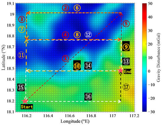
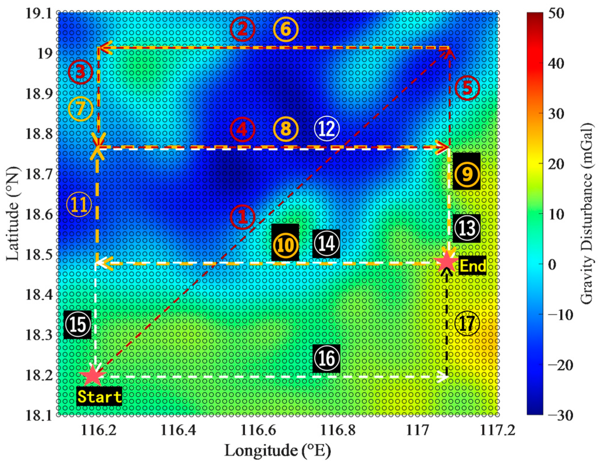
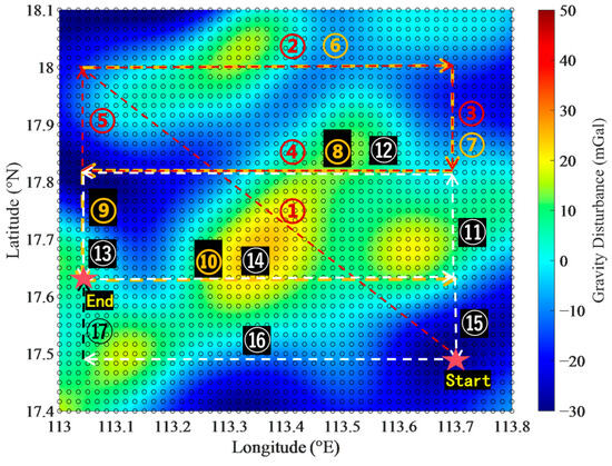
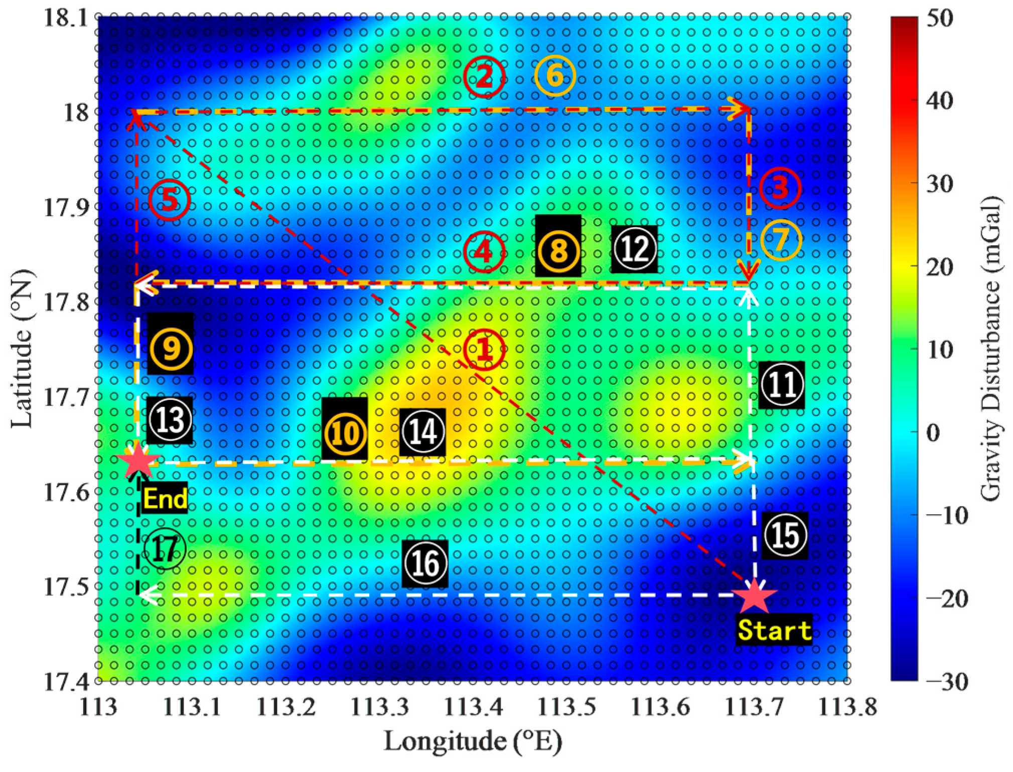
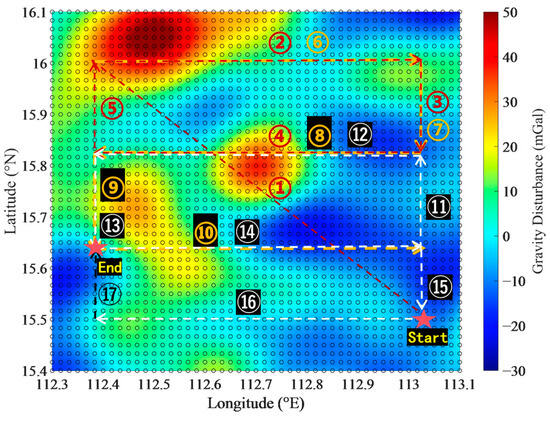
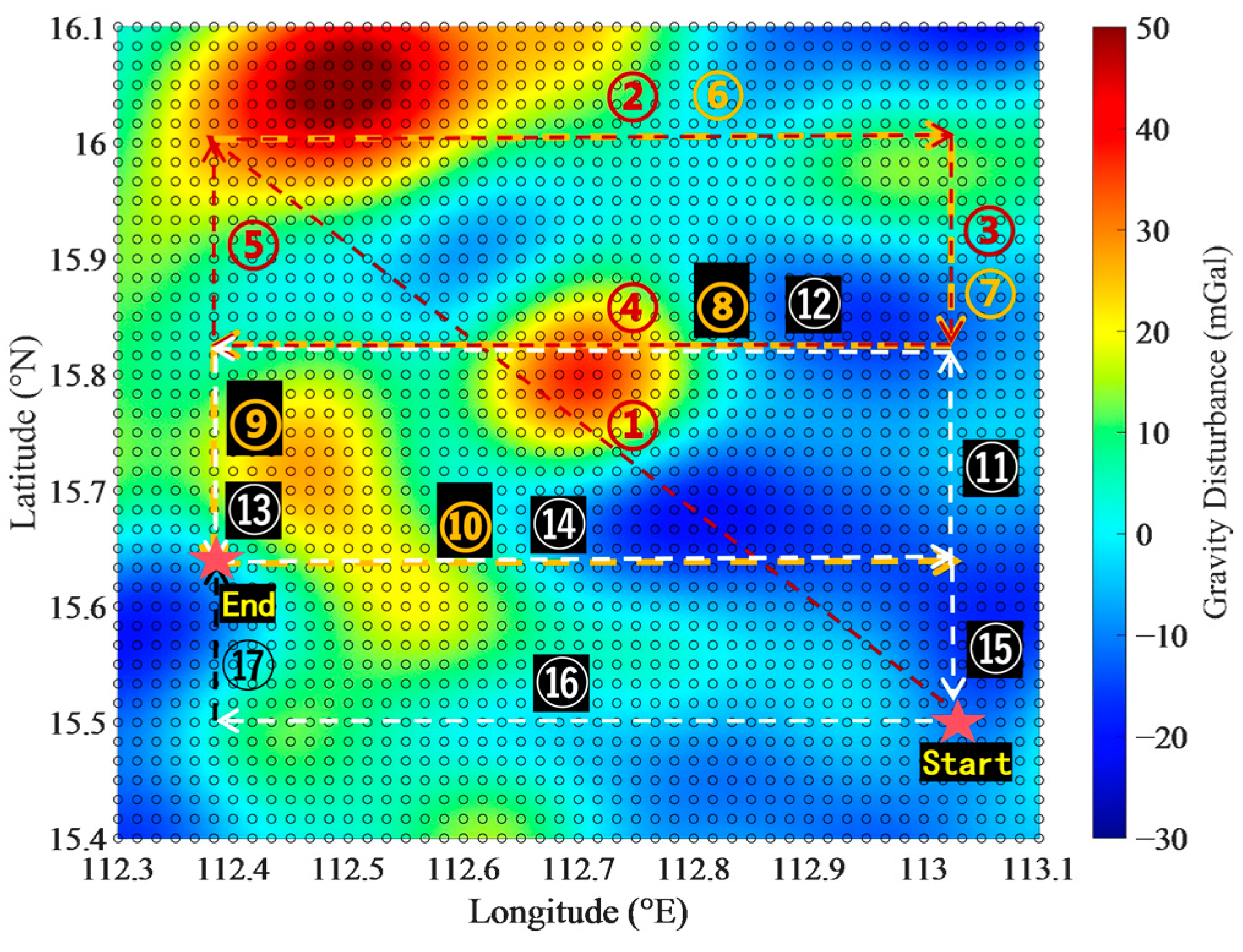
The sea trial was equipped with a high-precision laser inertial navigation system. The distribution of test sea areas and the ship’s navigation trajectory are presented in Figure 3, Figure 4 and Figure 5, with the numbers in the figure indicating the actual sailing sequence. The background map of gravity disturbance is generated from gravity disturbance values computed by the PAGravf4.5 software based on the 2159th-order EGM2008 global gravity field model.

Figure 3. Gravity Disturbance Distribution Heat Map—Test Sea Area #1 (mGal).

Figure 4. Gravity Disturbance Distribution Heat Map—Test Sea Area #2 (mGal).

Figure 5. Gravity Disturbance Distribution Heat Map—Test Sea Area #3 (mGal).

Through actual measurements with a gravimeter, the peak values of gravity disturbance in each sea area are 40 mGal, 50 mGal, and 95 mGal, respectively.

The trial compared the sea test results under these three different disturbance magnitude levels to verify the actual performance of the system in complex environments. To validate the practical performance of gravity disturbance compensation algorithms based on spherical harmonic models of different degrees, the EGM2008 gravity field model was adopted. Through the ICGEM platform, the gravity disturbance values from degree 2159 to degree 360 were calculated separately for the test area. The peak gravity disturbance values and data collection durations for each test sea area are shown in Table 3.

Table 3. Gravity Disturbance Peak Values.

Test Sea Area	1#	2#	3#
Measured Peak Gravity Disturbance (mGal)	40	50	95
2159-degree Gravity Disturbance Peak (mGal)	25.72	29.80	40.19
360-degree Gravity Disturbance Peak (mGal)	19.74	18.42	12.19
Data Collection Duration (h)	60	75	70

It can be observed that there are significant differences among the measured gravity disturbance, the 2159-degree gravity disturbance, and the 360-degree gravity disturbance. Affected by the smoothing effect of the model on local small-scale anomalies, the peaks of the 2159-degree model are generally lower than the measured values; the 360-degree model further truncates the high-frequency components, resulting in a more pronounced smoothing effect on local strong anomalies.

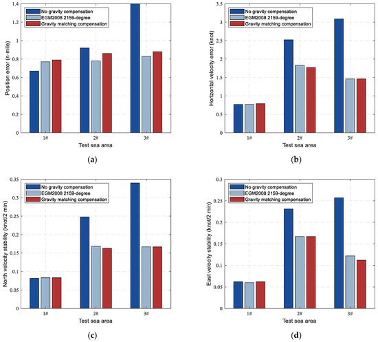
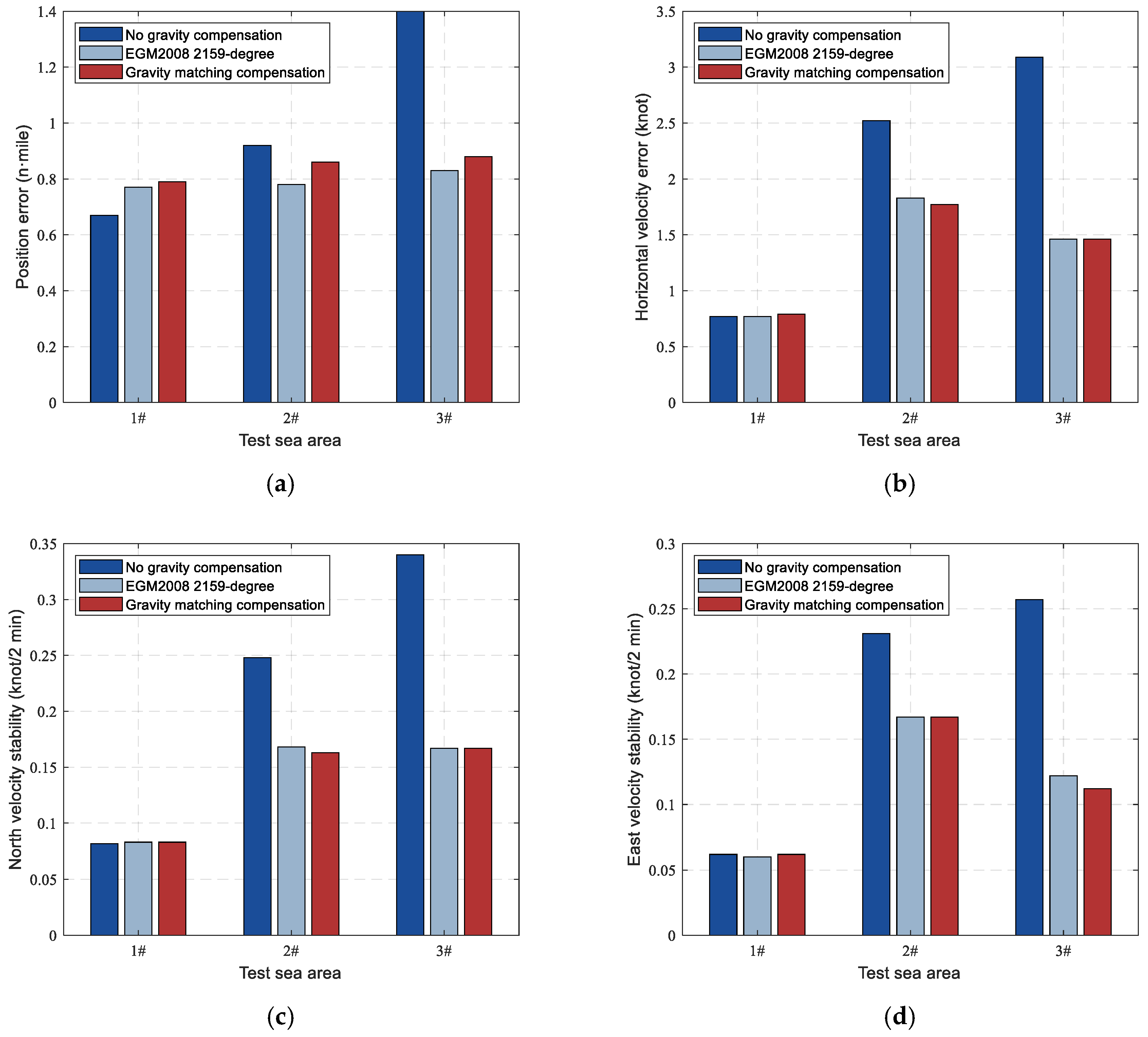
During the trial, position and velocity parameters were referenced against high-precision satellite navigation information, while heading lacked a reference source of equivalent accuracy. Therefore, the evaluation indicators of this trial primarily cover position error, horizontal velocity error, and velocity stability. The statistical results are shown in Figure 6, and the complete original statistical data of all working conditions are summarized in Appendix A.

Figure 6. Navigation performance comparison of different-degree gravity compensation methods in sea areas with varying gravity disturbance intensities. (a) Position error; (b) Horizontal velocity error; (c) North velocity stability; (d) East velocity stability.

4.2. Analysis of Compensation Results

From the experimental results, it can be directly observed that gravity disturbance and inertial navigation system errors exhibit a significant positive correlation: as the gravity disturbance in the sea area increases, the errors corresponding to various compensation algorithms show a clear upward trend.

A comprehensive comparison of the above multiple indicators reveals that the compensation effect of the 360-degree low-degree model is limited. In each test sea area, the navigation performance remains basically comparable to the uncompensated state, with no significant improvement in accuracy achieved. In contrast, the compensation effect of the 2159-degree high-degree model is overall superior, with navigation errors in the high-disturbance sea area (3# region) much lower than those without compensation and with the 360-degree model, resulting in a significant compensation gain.

However, the experimental data also indicate that high-degree gravity compensation models do not possess global universality. In the 1# region, the position error of the 2159-degree model (0.76 n·mile) is not only larger than that of the 360-degree model (0.72 n·mile) but even worse than the uncompensated state (0.67 n·mile), as shown in Figure 6, the position error curve for the 1# region.

To quantitatively analyze the differences in the representational capability of models of different degrees for the gravity field, the gravity disturbance difference $g_{diff}$ between the 2159-degree and 360-degree EGM2008 models within grid cell $i$ is first defined as:

$$g_{diff,i}=g_{2159,i}-g_{360,i}$$

(8)

where $g_{2159,i}$ and $g_{360,i}$ are the gravity disturbance values of the 2159-degree and 360-degree models within grid cell $i$, respectively. Table 4 presents the statistical results based on the difference matrix.

Table 4. Statistical Results of Gravity Disturbance Difference Values Between High- and Low-Degree Models in Each Test Sea Area.

Test Sea Area	1#	2#	3#
Root Mean Square (RMS) (mGal)	8.36	14.05	11.99
Standard Deviation (STD) (mGal)	8.41	13.00	10.94
Mean Deviation (mGal)	0.21	5.69	5.20

Among them, the Root Mean Square (RMS) and Standard Deviation (STD) directly reflect the degree to which the low-degree model fails to compensate for high-frequency, small-scale gravity anomalies. The calculation formulas are as follows:

$$RMS=\sqrt{{\displaystyle \frac{1}{N}}{\displaystyle \sum _{i=1}^N{(g_{diff,i})}^2}}$$

(9)

$$STD=\sqrt{{\displaystyle \frac{1}{N-1}}{\displaystyle \sum _{i=1}^N{(g_{diff,i}-\mu )}^2}}$$

(10)

where $N$ is the total number of grid points in the test sea area after dividing it into 1′ × 1′ grid cells (4087, 2107, and 2107 for Test Sea Areas #1, #2, and #3, respectively), and $\mu$ is the mean of the calculated differences.

Based on the data presented above, it can be observed that the gravity disturbance peak values of the 1# and 2# test sea areas are relatively close, at 40 mGal and 50 mGal, respectively. However, significant differences exist in the statistical representation of the differences. As can be seen from Table 4, the RMS and STD statistics of the 1# sea area are relatively small. From a mathematical perspective, the small statistical values indicate that the spatial distribution differences between the high- and low-degree models in this sea area are not pronounced.

In scenarios where the statistical differences in these difference values are relatively small, the high-degree model can provide effective fine-scale compensation, i.e., the high-frequency effective signal $g_{signal}$ is more prominent compared to the low-degree model. Theoretically, the calculation difference between the high- and low-degree models can be regarded as the superposition of the effective signal compensation and the high-degree truncation noise $g_{noise}$, that is,

$$g_{diff}=g_{signal}+g_{noise}$$

(11)

From the numerical perspective, the core mechanism by which the high-degree model captures more refined distribution features relies on high-degree polynomial fitting or high-degree differential operations applied to the data. However, real-world observational data from sea areas inevitably contain minor high-frequency environmental background noise or measurement errors. To quantitatively assess their influence, this subtle spatial high-frequency disturbance can be represented in the form of a simple harmonic wave:

$$\epsilon (x)=\delta \sin (\omega x)$$

(12)

where $\delta$ is the extremely small noise amplitude and $\omega$ is the high-frequency factor (typically $\omega \gg 1$). When the high-degree model performs $n$-th degree feature extraction on the data, according to the properties of micro-differentiation, the above disturbance term will evolve into:

$${\displaystyle \frac{{\partial }^n\epsilon (x)}{\partial x^n}}=\delta \cdot {\omega }^n\sin \left(\omega x+{\displaystyle \frac{n\pi }{2}}\right)$$

(13)

Extracting the amplitude magnitude shows that the numerical noise level introduced by the high-degree model, denoted as $\left|g_{\mathrm{noise}}\right|$, satisfies:

$$\left|\left.g_{noise}\right|\right.\propto \delta \cdot {\omega }^n$$

(14)

Equation (14) clearly reveals the mathematical essence of the high-degree amplification mechanism: since the high-frequency factor $\omega >1$, as the model degree $n$ increases, the originally weak underlying noise amplitude $\delta$ is dramatically amplified in a power-law manner by the factor ${\omega }^n$.

It should be noted that the above analysis is only a preliminary inference based on the current experimental data. The mechanism affecting the universality of high-order models is rather complicated. Apart from the noise amplification effect, it may also be related to marine terrain, ocean dynamic environment, truncation error of model order and other factors. This remains an open research issue, and we will further verify and improve relevant conclusions using measured data from more sea areas and voyages in follow-up work.

5. Conclusions

This paper investigates the compensation effects of gravity field models of different degrees on gravity disturbances in INS. Based on measured data from multiple sea areas and differential statistical analysis, it systematically reveals the representation laws of gravity field details by models of varying degrees. The study shows that although high-degree gravity field models, such as the 2159-degree model, possess higher theoretical resolution and generally provide superior compensation for gravity disturbances, they do not exhibit global universality in practical applications within local sea areas. The accuracy gains brought by increasing the model degree essentially depend on the degree of difference between the local real gravity field and the spherical harmonic model. When the differences in gravity field descriptions between high- and low-degree models are small in a local sea area, the compensation effect for high-frequency details becomes significantly insufficient; the truncation errors and computational noise introduced by the high-degree model may instead lead to degradation in model accuracy.

References

- Chang, L.; Qin, F.; Wu, M. Gravity disturbance compensation for inertial navigation system. IEEE Trans. Instrum. Meas. 2018, 68, 3751–3765. [Google Scholar] [CrossRef] [Scilit]
- Zha, F.; Wei, Q.; He, H. An Improved Error Modulation Scheme for Two-axis Rotation Inertial Navigation System. Fire Control Command Control 2023, 48, 180–186. [Google Scholar] [CrossRef]
- Yao, P.; Wu, D.; Xu, D.; Peng, J.; Chen, T.; Yang, G. A Rotational Modulation Method for the Rotational Inertial Navigation System of Long-Endurance Underwater Vehicle. IEEE Internet Things J. 2025, 12, 53914–53926. [Google Scholar] [CrossRef] [Scilit]
- Chen, H.; Wang, Z.; Sun, H.; Gu, D.; Miao, C.; Ye, W. Enhanced Dual-Axis Rotation Modulation Scheme for Inertial Navigation Systems Using a 64-Position Approach. Sensors 2026, 26, 1796. [Google Scholar] [CrossRef] [Scilit] [PubMed]
- An, W.; Xu, J.; Wu, M.; Li, F. Influence of gravity disturbance for SINS horizontal attitude. J. Natl. Univ. Def. Technol. 2021, 43, 135–141. [Google Scholar] [CrossRef]
- Li, S.Q.; Ouyang, Y.Z.; Chang, G.B.; Jin, J.H.; Li, K. Compensation technology of gravity disturbance vector in inertial navigation system. J. Chin. Inert. Technol. 2012, 20, 410–413. [Google Scholar] [CrossRef]
- Zhu, H.B.; Tian, Y.; Yan, G.M.; Li, S.H.; Liu, Z.P. Research on real-time gravity compensation system based on gravity model order adaptation. Navig. Position. Timing 2024, 11, 55–64. [Google Scholar] [CrossRef]
- Weng, J.; Liu, J.; Jiao, M.; Qin, Z.; He, X. Analysis and on-line compensation of gravity disturbance in a high-precision inertial navigation system. GPS Solut. 2020, 24, 83. [Google Scholar] [CrossRef] [Scilit]
- Yan, G.M.; Weng, L. Jielian Guandao Suanfa yu Zuhe Daohang Yuanli; Northwestern Polytechnical University Press: Xi’an, China, 2020. [Google Scholar]
- Zhang, P.; Wu, L.; Bao, L.; Wang, B.; Liu, H.; Li, Q.; Wang, Y. Gravity disturbance compensation for dual-axis rotary modulation inertial navigation system. Front. Mar. Sci. 2023, 10, 1086225. [Google Scholar] [CrossRef] [Scilit]
- Peng, J.C.; Wu, D. Schuler period oscillation error suppression for inertial navigation systems based on reverse and wavelet transforms. Measurement 2025, 242, 115862. [Google Scholar] [CrossRef] [Scilit]
- Guan, B.; Sun, Z.M.; Wu, F.M. Influence of horizontal components of disturbing gravity on position errors of inertial navigation system. Geomat. Inf. Sci. Wuhan Univ. 2017, 42, 1474–1481. [Google Scholar] [CrossRef]
- Pavlis, N.K.; Holmes, S.A.; Kenyon, S.C.; Factor, J.K. The development and evaluation of the Earth Gravitational Model 2008 (EGM2008). J. Geophys. Res. Solid Earth 2012, 117, B04406. [Google Scholar] [CrossRef] [Scilit]
- Tie, J.B. Research on Gravity Compensation in Inertial Navigation. Ph.D. Thesis, National University of Defense Technology, Changsha, China, 2018. [Google Scholar] [CrossRef]
- Zhang, C.J. The gravity responce in crust on different wavelength topography. Prog. Geophys. 2003, 18, 342–347. [Google Scholar] [CrossRef]
- Ince, E.S.; Barthelmes, F.; Reißland, S.; Elger, K.; Förste, C.; Flechtner, F.; Schuh, H. ICGEM—15 years of successful collection and distribution of global gravitational models, associated services, and future plans. Earth Syst. Sci. Data 2019, 11, 647–674. [Google Scholar] [CrossRef] [Scilit]
- Wang, J.; Yang, G.L.; Li, X.Y.; Zhou, X. Error indicator analysis for gravity disturbing vector’s influence on inertial navigation system. J. Chin. Inert. Technol. 2016, 24, 285–290. [Google Scholar] [CrossRef]
Disclaimer/Publisher’s Note: The statements, opinions and data contained in all publications are solely those of the individual author(s) and contributor(s) and not of MDPI and/or the editor(s). MDPI and/or the editor(s) disclaim responsibility for any injury to people or property resulting from any ideas, methods, instructions or products referred to in the content. |
© 2026 by the authors. Licensee MDPI, Basel, Switzerland. This article is an open access article distributed under the terms and conditions of the Creative Commons Attribution (CC BY) license.