


Abstract
In this work, we investigate deterministic chaos in external-cavity semiconductor lasers with delayed optical self-feedback. A noise-free quadrature-based delay differential model is used to isolate the intrinsic nonlinear dynamics produced by phase-sensitive delayed reinjection and carrier–photon interactions. Sensitivity to initial conditions is quantified by computing the leading Lyapunov exponents through a variational approach that integrates the base delay differential equations together with their delayed variational equations using a fourth-order Runge–Kutta method of steps and periodic QR orthonormalization. High-resolution Lyapunov maps are constructed in the parameter space for different pump ratios and selected short-feedback delays. The delay values are interpreted through the reference-normalized ratio , where is a fixed reference timescale derived from a reference solitary-laser operating point. The results show that both the spatial organization of positive- regions and the mean positive Lyapunov exponent are strongly affected by feedback delay, feedback phase, feedback strength, and pump ratio. Within the selected short-delay set, delayed self-feedback produces broader, more connected, and more strongly unstable chaotic regions as the external-cavity memory time increases toward the fixed reference timescale, particularly at larger pump ratios. These findings show that short external-cavity self-feedback can support robust deterministic chaotic regimes relevant to compact and integrated photonic implementations. The proposed framework provides a reproducible deterministic reference for identifying and interpreting feedback-induced chaos in short-delay external-cavity semiconductor lasers, while stochastic effects such as spontaneous-emission and Langevin noise are left for future robustness studies.
1. Introduction
Chaotic dynamics in semiconductor lasers with delayed optical feedback has been extensively studied as a canonical platform for high-dimensional nonlinear systems with memory. External-cavity semiconductor lasers (ECSLs) provide a compact and controllable realization of delay differential dynamics, where the reinjection of a time-delayed optical field fundamentally alters the phase-space structure and gives rise to a wide range of behaviors, including stable emission, periodic oscillations, quasiperiodicity, and fully developed deterministic chaos [1,2].
Although optical injection and delayed optical feedback are distinct physical configurations, both provide controllable routes to nonlinear and chaotic semiconductor-laser dynamics [3,4,5,6,7,8]. From a physical standpoint, the delayed optical feedback introduces an external timescale that competes with the intrinsic carrier–photon dynamics of the laser. This interaction leads to complex dynamical phenomena such as coherence collapse, low-frequency fluctuations, external-cavity modes, and chaotic itinerancy, which have been widely reported in both experimental and theoretical studies [9,10]. The resulting dynamics are inherently infinite-dimensional due to the presence of delay, making ECSLs a paradigmatic system for studying nonlinear dynamics in delay differential equations.
Beyond their fundamental interest, chaotic semiconductor lasers have enabled a wide range of applications in photonics and information processing. These include physical-layer secure communications using chaos masking and synchronization, high-speed true random number generation, microwave photonics, and neuromorphic computing based on reservoir dynamics [11,12,13,14,15,16,17,18,19,20]. In particular, recent advances in integrated photonics and long-haul optical transmission have demonstrated the scalability of chaotic carriers to high data rates and large distances, further motivating a deeper understanding of the underlying dynamical regimes [11,21,22,23,24,25,26].
Recent studies in nonlinear wave systems have also shown that rich spatiotemporal structures can emerge from the interaction of nonlinearity, external forcing, and nonautonomous effects. For example, Peregrine-type localized structures have been reported in nonautonomous partially nonlocal vector nonlinear Schrödinger models under harmonic potentials, illustrating the broader relevance of nonlinear-dynamical mechanisms in optical and wave-based systems [27]. In contrast, the present work focuses on a delayed-feedback semiconductor-laser configuration, where the dominant mechanism is the reinjection of the laser field after a short external-cavity delay.
Recent advances in laser and photonic technologies continue to expand the capabilities of modern optical systems. Examples include high-power thin-disk oscillators [28], mode-locked fiber lasers based on emerging saturable absorbers [29], broadband nonlinear optical sources for mid-infrared generation [30], and novel two-dimensional materials for ultrafast photonic applications [31]. Within this broader photonic landscape, semiconductor lasers remain particularly attractive for nonlinear dynamics and chaos studies because of their compactness, direct electrical pumping, strong carrier–photon coupling, high-speed modulation capability, and compatibility with integrated photonic platforms.
Semiconductor lasers operating in the 1550 nm wavelength region play a central role in modern photonic systems due to their compatibility with low-loss optical fiber transmission and their ability to provide compact, electrically pumped, and highly integrable light sources. Compared with other laser platforms, such as thin-disk, solid-state, dye, and fiber lasers, semiconductor lasers offer distinctive advantages including small footprint, high-speed direct modulation, wafer-scale manufacturability, and seamless integration with electronic and photonic integrated circuits. These characteristics have made semiconductor lasers key enabling devices in optical communications, microwave photonics, optical sensing, neuromorphic photonics, photonic reservoir computing, and secure communication systems. Understanding the nonlinear dynamics induced by delayed optical feedback is therefore important not only from a fundamental perspective but also for the design and optimization of advanced photonic technologies.
Despite decades of research, the precise structure of the parameter space leading to robust and broadband chaos in ECSLs remains only partially understood. The dynamics depend sensitively on multiple interacting parameters, including feedback strength, feedback phase, delay time, and pump level. While numerous studies have explored bifurcation diagrams and time-series behavior, systematic high-resolution mappings of chaos indicators across multidimensional parameter spaces are still limited, particularly for deterministic (noise-free) models.
A key aspect that has received comparatively less attention is the role of short feedback delays relative to sub-nanosecond carrier–photon timescales of the laser. In compact or integrated external-cavity configurations, the feedback path can become comparable to sub-nanosecond intrinsic laser timescales, making the delayed field capable of strongly modifying the stability and nonlinear response of the device. In this work, the selected delays are interpreted through the reference-normalized short-delay ratio , where is the relaxation-oscillation period associated with a previously characterized reference operating point. This provides a practical normalization for comparing short-feedback regimes without implying a complete pump-dependent resonance scan.
In this work, we investigate the emergence of chaos in an ECSL model with delayed optical feedback using a fully deterministic and variational framework. The system is described by delay differential equations in quadrature form, and the largest Lyapunov exponent is computed through the simultaneous integration of the system dynamics and its associated variational equations. This approach avoids phase-space reconstruction and provides a direct and high-resolution characterization of chaotic regimes.
Compared with previous chaos-analysis studies based on optically injected semiconductor lasers, the present work focuses on a physically distinct delayed self-feedback configuration in which the laser field is reinjected after a short external-cavity delay rather than driven by an independent master laser. The central novelty is therefore not the use of Lyapunov exponents or parameter-space maps alone, but the systematic characterization of the short-delay regime –, where the external-cavity memory time becomes comparable to the fixed reference timescale used for normalization. In this regime, the maps reveal that delayed self-feedback can generate broader and more connected positive Lyapunov-exponent regions as the delay increases within the selected short-delay set toward , particularly for larger pump ratios.
Thus, the main physical contribution of this work is the identification of how short delayed self-feedback, expressed relative to the fixed reference timescale , reorganizes the chaotic parameter space of ECSLs. Unlike optically injected lasers, where nonlinear dynamics are driven by the interaction between master and slave fields, the present configuration produces chaos through the reinjection of the laser field after a short external-cavity delay. This feedback-memory mechanism leads to a delay-dependent enlargement and structuring of chaotic regions in the parameter-space maps, showing that short external cavities compatible with compact or integrated photonic implementations can support strongly chaotic operating regimes.
The present work builds on the semiconductor-laser parameter set and reference relaxation-oscillation timescale used in Ref. [8], but it addresses a different physical configuration. Ref. [8] studied chaos in an optically injected semiconductor laser, where the nonlinear dynamics are driven by an independent external optical field. Here, the system is an external-cavity semiconductor laser with delayed optical self-feedback, in which the laser reinjects its own field after a finite delay, as shown in Figure 1.
Figure 1.
External-cavity semiconductor laser with delayed optical self-feedback.
This distinction changes both the governing equations and the relevant control parameters. In the optically injected case, the dynamics are organized by injection strength and frequency detuning. In the present delayed self-feedback problem, the dynamics are organized by feedback strength, feedback phase, feedback delay, and pump ratio. Therefore, the present manuscript extends the previous parameter baseline to a different delay differential feedback system and focuses on how short feedback memory reorganizes the chaotic operating regions in the plane.
The contributions of this work can be summarized as follows:
- We compute high-resolution Lyapunov maps of ECSLs across feedback strength and feedback phase, resolving fine dynamical structures in the parameter space.
- We employ a quadrature-based variational Lyapunov analysis for delay differential systems, enabling deterministic identification of chaotic regimes directly from the governing equations.
- We show that the reference-normalized short-delay ratio is a useful organizing parameter for comparing the selected short-feedback regimes.
- We show that, within the selected short-delay set, increasing feedback memory time toward the fixed reference timescale leads to broader, more connected, and more strongly unstable chaotic regions in the maps, especially at larger pump ratios.
The remainder of this paper is organized as follows. Section 2 introduces the ECSL model and the numerical framework used to compute Lyapunov exponents. Section 3 presents the chaos maps, interprets them in terms of the reference-normalized short-delay ratio, and discusses the implications of the results in relation to previous studies. Finally, Section 4 summarizes the main conclusions.
2. Method
To isolate the deterministic skeleton of the ECSL dynamics in numerical simulations, we neglect spontaneous-emission and Langevin noise terms, which introduce stochastic perturbations that can mask the intrinsic nonlinear behavior of the delayed-feedback system [1,3]. These noise sources reduce reproducibility, blur phase-space structures, and contaminate standard chaos indicators such as Lyapunov exponents, correlation dimension, and spectral features [32,33]. A similar deterministic/noise-aware separation is relevant in optically injected semiconductor lasers, where noise can modify pulsing statistics and complicate the interpretation of nonlinear regimes [34]. In their presence, nearby trajectories may diverge irregularly and autocorrelation functions can approach white-noise-like behavior, making it difficult to distinguish deterministic chaos from purely stochastic fluctuations. By suppressing noise at this stage, we ensure that the observed complexity arises primarily from deterministic feedback mechanisms, such as phase-sensitive delayed coupling and carrier–photon nonlinear interactions, providing a clean reference framework for the analysis of chaotic regimes.
The resulting Lyapunov maps should therefore be interpreted as deterministic reference maps that reveal the underlying organization of the ECSL parameter space in the absence of stochastic perturbations. In practical semiconductor lasers, spontaneous-emission and Langevin noise are unavoidable and may broaden stability boundaries, smooth narrow dynamical transitions, modify pulsing statistics, and affect the numerical value of the Lyapunov exponents, particularly near marginal regions where . Consequently, the present results are not intended as a direct quantitative prediction of a specific experimental device, but rather as a characterization of the deterministic skeleton that underlies the delayed-feedback dynamics.
2.1. External-Cavity Semiconductor Laser (ECSL): Quadrature Model (Self-Feedback)
We consider the normalized ECSL dynamics in the quadrature variables and , defined through the complex field envelope
together with the carrier variable . The system includes delayed self-feedback with delay , effective feedback rate , and constant feedback phase offset .
Define the real gain factor
and rotate the delayed field according to
The quadrature ECSL equations read
The measured intensity is
In this rotating frame, the system is an autonomous delay differential equation (DDE), since the feedback term depends only on the delayed state.
Variational Equations (For Lyapunov Exponents)
Equation (4) can be written compactly as
The corresponding delayed variational system is
where
evaluated along the base trajectory. Let and . Using and , the Jacobian with respect to the undelayed state is
and the Jacobian with respect to the delayed state is
These Jacobians contain no divisions by the field amplitude and therefore provide a numerically robust basis for the computation of Lyapunov exponents.
2.2. RK4 Integration for the Quadrature ECSL DDE and Its Variational Equations
The numerical procedure combines a classical fourth-order Runge–Kutta method of steps for the base trajectory with a synchronized RK4 integration of the delayed variational system and periodic QR orthonormalization for Lyapunov-exponent accumulation. In the actual implementation, the DDE tangent dynamics are represented through an explicit discretized history of perturbation blocks rather than through a single tangent matrix with an abstract delay operator.
2.2.1. Time Discretization and Initial Conditions
The total simulation time is discretized as
with a uniform step
For the base trajectory, the initial history is taken as a constant no-feedback steady state. Specifically,
and the quadrature initial condition is chosen as
which corresponds to selecting zero initial optical phase. The constant history is therefore prescribed as
The same constant initial history was used for all parameter points in order to define a reproducible deterministic protocol for comparing the Lyapunov maps. Therefore, the reported exponents characterize the asymptotic dynamics reached from this prescribed history and should not be interpreted as a complete basin-of-attraction analysis.
For a given delay , the number of delay steps is defined as
The tangent history is stored in an extended matrix
organized as stacked blocks,
At the beginning of each parameter run, this matrix is initialized as
Thus, the current perturbation basis occupies the first block, and the delayed tangent history is initially zero.
The use of three tangent directions should therefore be understood as a dominant-subspace Lyapunov calculation rather than as a truncation of the delayed state variables. The delayed perturbations are evolved inside the discretized history space of dimension , but only three independent perturbation columns are retained because the objective is to estimate the leading exponents, especially . For the purpose of identifying chaos through the sign of the maximum Lyapunov exponent, a complete orthonormal basis of the discretized history space is not required. A generic perturbation direction with nonzero projection onto the most unstable tangent direction converges asymptotically to the leading Lyapunov exponent under the standard tangent-space formulation for finite-dimensional systems and its extension to delay systems [35,36,37].
Consequently, the reported values should be interpreted as estimates of the leading Lyapunov exponents associated with the evolved perturbation subspace, not as the full spectrum of the delay system. This distinction is important because quantities that depend on the complete spectrum, such as the full Lyapunov dimension of the infinite-dimensional DDE, are outside the scope of the present work. The classification of chaotic regions, however, relies only on the sign of , which is the most robust quantity obtained from the dominant tangent dynamics.
2.2.2. Method of Steps for the Base Trajectory
The base trajectory is stored as a discrete history, and delayed states are obtained by linear interpolation. Let denote this interpolation operator. At time step , the delayed RK4 stage states are
with the classical RK4 abscissae
If the delayed argument satisfies , the constant initial history is used. Otherwise, the delayed state is recovered by linear interpolation of the stored trajectory samples. This is exactly the rule implemented in the history function used by the code.
The RK4 stages for the base DDE are then computed as
followed by the standard update
Non-finite states are treated as numerical failure for that parameter point.
2.2.3. Variational RK4 with Explicit Delayed Tangent History
The variational dynamics are not integrated from the beginning of the run. Instead, a warm-up interval is introduced, and the tangent evolution starts only when
At each step, the current perturbation block is extracted as
To evaluate delayed perturbations at intermediate RK4 stages, a second interpolation operator is defined over the extended tangent history. For the stage abscissae , the delayed perturbation blocks are
In practice, this interpolation is performed linearly between neighboring blocks in the stacked matrix , using the delay lag measured in units of the time step h. If the requested delayed time falls beyond the stored history, the oldest available block is used.
The synchronized RK4 stages of the variational system are then computed as
where
The current perturbation block is updated as
After this update, the entire extended tangent history is shifted one block backward and the newly computed perturbation block is inserted at the top:
This explicit block-history update is the actual delayed-tangent representation used by the implementation.
2.2.4. QR Orthonormalization and Lyapunov Accumulation
Lyapunov accumulation does not start immediately after the tangent warm-up. A second threshold time is imposed, and accumulation begins only when
At the first step satisfying this condition, the extended tangent matrix is orthonormalized through a reduced QR decomposition,
the logarithmic accumulators are reset, and subsequent renormalizations are performed every time steps. At each renormalization event,
Very small diagonal entries are clipped to a lower bound before taking logarithms in order to avoid numerical underflow.
If denotes the set of renormalization indices after the transient, the Lyapunov exponents are estimated as
with total accumulation time
Only the three leading exponents are retained for each parameter point. If no valid renormalization event occurs after the transient, the corresponding Lyapunov exponents are marked as undefined.
The procedure is repeated over the selected parameter grid. For each coupling value C, the effective feedback coefficient is computed as
and the three Lyapunov exponents are stored as functions of for the construction of the corresponding chaos maps.
This formulation avoids the singular terms present in the phasor model and implements the delayed variational dynamics through an explicit discretization of the tangent history, ensuring numerical stability in the computation of Lyapunov exponents.
It is important to note that, because the ECSL model is a delay differential equation, its exact phase space is infinite-dimensional. Therefore, the extended tangent-history matrix
should not be interpreted as a representation of the full Lyapunov spectrum of the infinite-dimensional DDE. Instead, it provides a finite-dimensional discretized history representation used to evolve three independent tangent perturbation directions and estimate the three dominant Lyapunov exponents. In this sense, the QR procedure is applied to three tangent vectors embedded in the discretized history space, allowing the leading exponents to be tracked consistently along the delayed trajectory. The objective of this work is therefore not to compute the complete infinite-dimensional Lyapunov spectrum of the DDE, but to obtain a robust estimate of the leading exponents, especially , which is sufficient for identifying chaotic regions through the criterion .
Algorithm 1 summarizes the numerical workflow used for the quadrature ECSL model.
| Algorithm 1 Quadrature ECSL Lyapunov computation |
| 1: Initialize |
| 2: Initialize |
| 3: Initialize and set |
| 4: Compute |
| 5: Set startedAccum ← false |
| 6: for do |
| 7: |
| 8: Compute by interpolation |
| 9: Compute RK4 stages |
| 10: Update and store in |
| 11: if then |
| 12: |
| 13: Compute by interpolation |
| 14: Evaluate at RK4 stages |
| 15: Compute |
| 16: Update |
| 17: Shift and insert into first block |
| 18: if and not startedAccum then |
| 19: QR-orthonormalize , reset accumulators |
| 20: startedAccum ← true |
| 21: end if |
| 22: if startedAccum and then |
| 23: QR-orthonormalize |
| 24: Accumulate |
| 25: end if |
| 26: end if |
| 27: end for |
| 28: if valid QR events exist then |
| 29: Compute |
| 30: else |
| 31: Set |
| 32: end if |
To verify that the reported Lyapunov maps are not artifacts of the selected time discretization, numerical convergence tests were performed using three integration time steps: , , and . For each case, the maximum Lyapunov exponent , the remaining leading exponents, the fraction of chaotic parameter space defined by , and the spatial structure of the resulting chaos maps were compared. The results were found to be practically unchanged when reducing the time step below . In particular, the locations of the positive- regions, the qualitative organization of the chaotic domains, and the computed chaotic fractions remained essentially invariant. Smaller time steps only increased the computational cost substantially, without producing meaningful changes in the Lyapunov spectra or in the resulting stability boundaries. Therefore, was adopted as the reference time step for the parameter sweeps, as it provides a suitable compromise between numerical accuracy and computational efficiency.
Additional numerical sensitivity tests shown in Table 1 were performed to verify that the reported Lyapunov maps are robust with respect to the main numerical parameters of the integration and Lyapunov-accumulation procedure. In particular, we tested the total integration time, the discarded transient time, the Lyapunov accumulation time, the QR reorthonormalization interval, the interpolation scheme used for the delayed history, and the resolution of the parameter grid. In all cases, the sign structure of the maximum Lyapunov exponent, the fraction of chaotic parameter space defined by , and the spatial organization of the chaotic domains remained practically unchanged. The numerical refinements mainly increased the computational cost without producing meaningful changes in the stability boundaries or in the qualitative structure of the chaos maps.
Table 1.
Numerical sensitivity tests used to validate the robustness of the variational Lyapunov maps.
These tests indicate that the reported chaos maps are numerically converged for the selected reference configuration. Therefore, the final parameter sweeps were performed using , the reference transient and accumulation times, and the selected grid resolution, since further numerical refinement increased the computational cost without modifying the physical conclusions.
These tests support the robustness of the leading-exponent classification used in this work, while the computation of a complete high-dimensional delay spectrum would require a substantially larger tangent basis and is not attempted here.
2.2.5. Notes on Parameters and Numerics
The main control axes for the numerical ECSL chaos maps are the dimensionless feedback strength , with , and the feedback phase , which can be scanned by small variations of the laser current or temperature that modify the optical frequency while keeping the external-cavity delay fixed. The delay sets the fundamental external-cavity time scale and determines the memory depth of the system.
In the numerical maps, the feedback phase is treated as an independent effective phase parameter of the delayed feedback loop. For a fixed delay, a full phase change corresponds to an optical-frequency shift . Thus, for , one obtains , while the shorter delays require proportionally larger frequency shifts.
Although such frequency shifts can be approached through current or temperature tuning in semiconductor lasers, these tuning mechanisms may also modify the carrier density, gain, and operating point. Therefore, the phase scan used here should be interpreted as an idealized effective-feedback-phase sweep. In experimental or integrated photonic implementations, could also be controlled by changing the feedback-path length, using a thermo-optic or electro-optic phase shifter, or tuning the external feedback section, rather than by changing the laser operating current alone.
For reproducible and noise-free simulations, a prescribed history function is defined on the interval . The integration time step was chosen to be sufficiently small to resolve the feedback delay, the relaxation-oscillation timescale, and the photon lifetime. Linear interpolation is employed for all delayed evaluations in the RK4 substeps of both the base trajectory and the variational equations, consistent with the discrete method-of-steps implementation. Since the integration step is small compared with the relevant dynamical time scales, , further refinements to and produced practically unchanged Lyapunov spectra and chaos maps. Therefore, the use of linear interpolation provides an adequate compromise between numerical accuracy and computational cost.
All simulations reported in this work correspond to the deterministic external-cavity semiconductor laser (ECSL) model with delayed optical feedback. The laser parameters listed in Table 2 were selected to represent typical single-mode semiconductor lasers operating at (1.55 μm) and are consistent with values commonly reported in the literature [38,39]. No optical injection terms are included, and all coupling effects arise exclusively from delayed self-feedback.
Table 2.
Physical laser parameters used in the ECSL delayed-feedback model. The values are representative of single-mode semiconductor lasers operating near and are consistent with parameters commonly reported in the literature [38,39].
In the present real-amplitude formulation, all optical reflectivities are incorporated into the effective feedback gain through the product
which fully determines the strength of the delayed feedback. is an effective feedback rate (s−1), and accounts for the amplitude transmission of the external feedback loop, including propagation losses and coupling efficiencies. Both parameters are phenomenological and represent a lumped description of the physical processes occurring at the laser facet, the external coupler, and the feedback reflector.
To make contact with a more explicit physical interpretation, one may express the feedback strength as
where is the internal round-trip time of the laser cavity, is the amplitude reflectivity of the laser facet through which the feedback is extracted, is the amplitude reflectivity of the external feedback mirror (or equivalent reflector), and represents the amplitude attenuation accumulated along the external feedback path due to propagation losses, imperfect coupling, or scattering. The dimensionless function collects the facet and coupler coupling efficiency, translating the internal cavity field into the external feedback field and back into the laser.
The dimensionless feedback strength used in the maps can be interpreted through the relation as shown in Table 3. Since the photon lifetime used in this work is , the nominal sweep range corresponds to an effective feedback rate
The displayed Lyapunov maps report the numerically convergent portion of this nominal sweep, extending up to approximately (). Thus, values near represent weak delayed feedback, values in the approximate range represent moderate feedback, and values approaching represent strong or very strong feedback in the present normalization.
Table 3.
Order-of-magnitude interpretation of the dimensionless feedback strength used in the Lyapunov-map sweep. The classification is given in the normalization of the present ECSL model.
Using
one sees that a given value of C can be reached through different combinations of internal round-trip time, facet coupling, feedback-loop transmission, and external reflector amplitude. For compact photonic feedback paths, weak-to-moderate values of C are compatible with partial external reflection and realistic propagation or coupling losses. In contrast, the upper end of the sweep, , should be regarded as a strong-feedback limit that may require high feedback-loop transmission and large effective external reflectivity.
For a simple facet-mirror external cavity configuration, following the standard Lang–Kobayashi boundary conditions, this coupling factor can be written explicitly as
which corresponds to the ratio between the transmitted and internally reflected field amplitudes at the laser facet. Substituting this expression into the feedback strength yields
Within this formulation, the parameters used in the dynamical equations are related as
so that incorporates the facet reflectivity and external reflector properties, while captures the amplitude transmission of the feedback loop. The feedback phase naturally includes the optical phase accumulated during propagation in the external cavity and any additional phase shifts introduced by reflections at the laser facet and the external reflector.
This decomposition clarifies how the normalized feedback parameters used in the ECSL model can be consistently connected to physically meaningful quantities such as facet reflectivities, external mirror reflectivity, propagation losses, and optical path length in the feedback loop.
The facet reflectivity on the side opposite to the external cavity, denoted by , is absorbed into the internal laser parameters through the photon decay rate and the normalization of the field amplitude, and therefore does not appear explicitly in the feedback term.
In the present normalized formulation, the internal cavity losses and output coupling through the laser facet are absorbed into the photon decay rate and into the normalization of the field amplitude . Let denote the amplitude reflectivity of the output facet of the laser cavity. The photon decay rate can be written as
where is the internal round-trip time of the cavity, and accounts for internal distributed losses (waveguide absorption, scattering, etc.). The term represents the photon loss associated with transmission through the output facet.
In the limit of weak losses, this expression can be approximated as
showing explicitly that the facet reflectivity directly controls the photon lifetime and therefore the damping of the intracavity field.
The normalization of the real field amplitude is chosen such that the intracavity photon number is proportional to . Under this convention, the power emitted through the output facet is proportional to
so that the same reflectivity parameter simultaneously determines the extraction efficiency of the laser output and contributes to the total photon decay rate appearing in the carrier–photon rate equations.
Therefore, in the ECSL model the facet reflectivity enters implicitly through the following:
- The photon decay rate , which fixes the photon lifetime and the relaxation-oscillation frequency;
- The normalization of the field amplitude , through the proportionality between and the emitted optical power.
This treatment is consistent with standard rate-equation models of semiconductor lasers, where individual cavity mirror reflectivities are not introduced explicitly, but are instead incorporated into the effective photon loss rate and the normalization of the intracavity field.
2.3. Selection of Short-Delay Values
The feedback-delay values used in this work were selected relative to the relaxation-oscillation timescale of the reference laser configuration. In our previous chaos analysis [8] of the same semiconductor-laser parameter set, the relaxation oscillation frequency was obtained as
for the reference operating point . This corresponds to a relaxation-oscillation period
The derivation of this estimate from the small-signal intensity–carrier dynamics is summarized in Appendix A.
The use of from Ref. [8] is intended only to provide a common reference timescale for the same semiconductor-laser parameter set. It does not imply that the present delayed-feedback system is dynamically equivalent to the optically injected system studied previously. In the present work, the reference period is used to express the selected short feedback delays on a comparable timescale, while the actual dynamics are generated by delayed self-feedback.
Because the relaxation-oscillation frequency depends on the pump current, the reference value should not be interpreted as the actual relaxation period for all simulated pump ratios. It is used here as a fixed reference timescale associated with the previously characterized operating point . To avoid ambiguity, Table 4 reports the pump-dependent relaxation frequencies and periods estimated from the same small-signal expression used in Appendix A.
Table 4.
Pump-dependent relaxation-oscillation frequencies and periods estimated using the same small-signal expression employed in Appendix A. The value corresponds to the reference operating point , not to the pump ratios used in the Lyapunov maps.
With respect to the pump-dependent relaxation periods, the simulated delay ratios are therefore smaller than unity. For , the ratios are approximately , , and ; for , they are approximately , , and ; and for , they are approximately , , and . Thus, the selected feedback delays remain in the short-delay regime relative to the actual pump-dependent relaxation periods. The ratio is therefore used only as a fixed reference coordinate, not as a pump-dependent resonance condition.
Based on this reference timescale, we selected three short external-cavity delays,
These values probe delayed-feedback memory times ranging from approximately one half of the fixed reference timescale to one full fixed reference timescale. Specifically,
This short-delay range is of particular interest because it is compatible with compact external-feedback paths and therefore relevant to future implementations in integrated photonic platforms. In such systems, the optical feedback cavity must remain sufficiently short to be physically realizable on chip or in hybrid integrated configurations. The purpose of the present delay selection is therefore not to perform an exhaustive delay scan, but to examine how deterministic chaos emerges when the external feedback memory time becomes a substantial fraction of the fixed reference timescale used for normalization.
Advantages of the Variational Method
The variational method provides deterministic, high-resolution estimation of Lyapunov exponents without relying on phase-space reconstruction or embedding parameters. Unlike approximate time-series techniques such as the method of Rosenstein et al. [40], the variational approach exploits the governing equations and their analytical derivatives, following the standard tangent-space framework for Lyapunov-exponent computation [35,36]. This makes it particularly well suited for the ECSL, where an accurate and noise-free characterization of stability and chaotic regimes must be derived from the intrinsic deterministic dynamics of the optical feedback.
3. Results
The dynamical behavior of the external-cavity semiconductor laser (ECSL) was systematically investigated through two-dimensional Lyapunov maps in the parameter space defined by the dimensionless feedback strength C, displayed as , and feedback phase . The maximum Lyapunov exponent was computed using the proposed variational delay differential framework combined with periodic QR re-orthonormalization, providing a deterministic classification of chaotic and non-chaotic parameter regions. The nominal feedback-strength sweep covered , but the maps shown below display only the numerically convergent portion of the sweep, extending up to approximately ().
Three representative short-feedback delays were analyzed as shown in Table 5:
These values were selected relative to the fixed reference timescale
obtained from the reference solitary-laser operating point , as described in Appendix A. Therefore, the normalized short-delay ratios explored in this work are approximately
This choice allows us to examine deterministic chaos generation in short external cavities whose memory time ranges from about one half of the fixed reference timescale to one full fixed reference timescale. Such short-delay regimes are particularly relevant for compact and potentially integrated photonic implementations, where the external feedback path must remain physically short.
Table 5.
Simulation and parameter-sweep configuration used to generate the ECSL Lyapunov maps. The sweep is organized in terms of pump ratio, feedback strength, feedback phase, and short external-cavity delay. The relaxation-oscillation quantities are based on the reference solitary-laser operating point and are used only to define the normalized short-delay ratio .
The analysis was performed for pump ratios
corresponding to operating conditions above threshold. Increasing enhances the carrier-induced gain and modifies the nonlinear coupling between the optical field and the carrier density, thereby influencing the onset and spatial organization of chaotic regions under delayed optical feedback.
Figure 2 presents the Lyapunov maps obtained for the three short-feedback delays and the three pump ratios considered. Regions with positive maximum Lyapunov exponent, , are classified as chaotic, while regions with are classified as non-chaotic within the deterministic Lyapunov criterion used in this work.
Figure 2.
Lyapunov maps of the maximum Lyapunov exponent for the selected short-feedback delays and pump ratios. Positive values of identify chaotic dynamics according to the variational Lyapunov criterion. The maps display the numerically convergent portion of the nominal feedback-strength sweep, extending up to approximately (). The maps show that the extent and organization of chaotic regions depend strongly on feedback delay, feedback phase, feedback strength, and pump ratio.
For the shortest delay, , the system remains predominantly non-chaotic over a large portion of the parameter space, particularly for . Only isolated and fragmented positive- regions are observed, indicating that the delayed feedback acts as a comparatively weak perturbation when the external-cavity memory time is about one half of .
As the pump ratio increases from to , positive- regions progressively emerge and expand. This trend indicates that stronger pumping enhances the sensitivity of the ECSL dynamics to delayed optical feedback. Nevertheless, for the shortest delay the chaotic regions remain relatively localized and disconnected.
For the intermediate delay, , the maps show a clear increase in dynamical complexity. Broader regions of positive Lyapunov exponent appear across the parameter space, revealing stronger sensitivity to both feedback strength and feedback phase. Compared with the shortest-delay case, the chaotic domains become more structured, suggesting a more effective interaction between the delayed optical field and the intrinsic carrier–photon dynamics.
The strongest positive-Lyapunov behavior among the selected cases is obtained for , which coincides with the fixed reference timescale . In this regime, large connected regions of positive Lyapunov exponent occupy significant portions of the parameter space, especially for and . This result indicates that, within the selected short-delay set, longer feedback-memory times relative to the fixed reference scale are associated with stronger delayed-feedback-induced instability.
3.1. Dependence on Normalized Short-Delay Ratio
To provide a compact interpretation of the delay dependence, the results were analyzed in terms of the normalized short-delay ratio
where is the fixed reference timescale defined in Appendix A. This normalization is not intended to represent a full pump-dependent resonance scan. Instead, it provides a common reference timescale for comparing the selected short external-cavity delays.
Because only three feedback-delay values were simulated, the normalized short-delay ratio should be interpreted as a reference coordinate for comparing the selected cases, not as a complete delay-dependent control parameter. Thus, provides a physically meaningful way to express the selected short external-cavity delays relative to the fixed reference timescale used for normalization, but it does not by itself establish a monotonic or resonance-driven dependence of the chaotic fraction on delay.
Figure 3 summarizes the mean positive maximum Lyapunov exponent and the chaotic fraction as functions of the reference-normalized delay ratio . The chaotic fraction was computed as the ratio between the number of parameter points satisfying and the total number of parameter points represented in the corresponding Lyapunov map.
Figure 3.
Summary of the mean positive maximum Lyapunov exponent and chaotic fraction as functions of the reference-normalized delay ratio for the selected pump ratios. The figure compares only the selected short-delay cases and is not intended as a dense delay scan.
The increase in the mean positive Lyapunov exponent as increases toward the fixed reference value should therefore be interpreted with care. Since the actual relaxation period depends on , the selected delays do not correspond to for the simulated pump ratios. Instead, Figure 3 shows that, within the selected short-delay set, larger feedback-memory times relative to the fixed reference scale lead to stronger positive-Lyapunov dynamics. This observation does not establish a pump-dependent relaxation-resonance condition.
Figure 3 shows two complementary quantities: the mean positive maximum Lyapunov exponent and the chaotic fraction. The mean positive exponent increases as the feedback delay increases within the selected short-delay set toward the fixed reference timescale , particularly for larger pump ratios. This indicates that, within the chaotic regions that are present, the trajectories become more strongly unstable. In contrast, the chaotic fraction does not vary monotonically over the three simulated delays. This non-monotonic behavior indicates that the area occupied by chaotic regions in the parameter space is controlled not only by the delay, but also by the feedback phase, feedback strength, and pump ratio.
The intermediate case therefore should not be interpreted as evidence of a simple resonance trend. Instead, it shows that short-delay feedback can reorganize the parameter-space morphology, reducing the fraction of chaotic points in some pump cases while still producing stronger instability within the chaotic regions that remain. A denser sweep over would be required to resolve delay-dependent branches, subharmonic windows, or bifurcation sequences.
Accordingly, the main conclusion drawn from the normalized-delay analysis is limited to the selected short-delay set: as the feedback memory time increases toward the fixed reference timescale , the simulated maps exhibit stronger positive-Lyapunov dynamics, while the spatial fraction of chaotic parameter space shows a non-monotonic dependence on delay. This supports the use of as a useful organizing coordinate for the selected cases, but not as proof of a complete resonance structure.
Although the ECSL model and the variational Lyapunov calculation are formulated in the quadrature variables , the representative attractors in Figure 4 are displayed in amplitude-phase coordinates only for visualization. The optical amplitude and optical phase were computed as
This is equivalent to first computing the wrapped phase in (−π, π) using atan2 and then unwrapping it in time to remove artificial 2π phase discontinuities. This amplitude-phase representation is not used in the numerical integration or in the Lyapunov exponent calculation.
Figure 4.
Representative chaotic trajectories for two parameter points located inside positive- regions. Panels show attractor projections in and the corresponding intensity traces . (a) Attractor projection in the phase space for = 1.5 rad and C = 10−1.5. (b) Corresponding intensity trace for the parameters in (a). (c) Attractor projection in the phase space for = −1.5 rad and C = 10−1.4. (d) Corresponding intensity trace for the parameters in (c). These plots provide qualitative visualization of the chaotic regimes identified quantitatively by the Lyapunov analysis.
The attractor projections in Figure 4 therefore provide only a qualitative visualization of representative chaotic trajectories; the classification of chaos is based exclusively on the sign of the maximum Lyapunov exponent computed in the quadrature variables.
Figure 4 provides representative time-domain and phase-space evidence for two parameter points selected inside regions with clearly positive maximum Lyapunov exponent. Both examples correspond to and , where the Lyapunov maps indicate strongly chaotic dynamics. The attractors in Figure 4a,c exhibit irregular, non-closed trajectories in the space. Figure 4a corresponds to and , while Figure 4c corresponds to and . The corresponding intensity traces in panels Figure 4b,d, computed as , show nonperiodic pulsations with irregular peak amplitudes and variable temporal spacing. These visual signatures are consistent with the positive- classification obtained from the variational Lyapunov analysis. The attractor projections and intensity traces are not used as the primary chaos criterion; rather, they provide complementary dynamical examples of the regimes identified quantitatively by the condition .
3.2. Discussion
The results demonstrate that the external-cavity delay plays a central role in shaping the nonlinear dynamics of the ECSL system. For the shorter selected delays, the delayed optical field produces mainly localized chaotic regions in parameter space. In contrast, as the feedback delay increases within the selected short-delay set toward the fixed reference timescale , the feedback memory time becomes longer relative to the normalization scale, leading to broader and more organized positive- regions.
The qualitative structure of the maps is consistent with previous studies of semiconductor lasers operating in the short-cavity regime and with the known Lang–Kobayashi picture of delayed optical feedback [41,42,43,44,45,46,47]. In the short-cavity regime, the external-cavity delay can be comparable to intrinsic carrier–photon timescales, and the feedback phase becomes a critical control parameter for the stability of external-cavity modes and for the emergence of complex intensity dynamics. Similarly, in the Lang–Kobayashi framework, weak feedback first perturbs the solitary-laser state and external-cavity modes, whereas stronger feedback can destabilize these states through bifurcations leading to periodic, quasiperiodic, and chaotic dynamics. The present maps are consistent with these expected features: increasing feedback strength is associated with broader regions of positive maximum Lyapunov exponent, while variations of feedback phase produce alternating chaotic and non-chaotic domains, indicating that the delayed field can either reinforce or suppress the carrier–photon oscillations depending on its phase relation with the intracavity field.
Consequently, the axis in the Lyapunov maps represents controlled variation of the effective feedback phase under fixed model parameters; experimental scans based solely on current or temperature tuning may not keep all other laser parameters strictly constant.
The structure of the Lyapunov maps can be understood as the result of phase-sensitive delayed self-interference. For a fixed delay, changing the feedback phase modifies whether the reinjected field constructively or destructively interacts with the intracavity field. As a consequence, some regions of the parameter space favor the growth of carrier–photon oscillations and lead to positive Lyapunov exponents, whereas other regions stabilize periodic or quasiperiodic responses and appear as non-chaotic windows. Within the selected short-delay set, the enlargement of chaotic domains as the feedback delay increases toward the fixed reference timescale indicates that the delayed field becomes more effective at perturbing the carrier–photon exchange dynamics of the laser.
The boundaries between positive and non-positive Lyapunov regions should therefore be interpreted as transition zones between delayed-feedback-stabilized regular dynamics and broadband chaotic dynamics. The present maps identify these transition regions with high resolution, but they do not by themselves constitute a full bifurcation-continuation analysis. For this reason, we do not assign specific mechanisms such as crisis bifurcations or intermittency without additional continuation calculations. Instead, the representative attractors and intensity traces provide complementary dynamical evidence showing how selected positive-Lyapunov regions correspond to irregular phase-space trajectories and nonperiodic optical pulsations.
Additional dynamical indicators, including the correlation dimension, the zero-one test for chaos, power spectra, and autocorrelation functions, could provide further insight into the detailed transition mechanisms at the boundaries of the chaotic regions. In the present work, the variational maximum Lyapunov exponent is retained as the primary chaos indicator because it is computed directly from the governing equations and their delayed variational dynamics. Future work may combine the present Lyapunov-map framework with these complementary diagnostics to classify periodic windows, intermittency routes, and possible crisis-like transitions in greater detail.
It should be noted that the largest values of C included in the sweep correspond to a strong-feedback regime in the present normalization. These points are useful for identifying the extent of the chaotic domains and for determining how the maps evolve as feedback increases. However, the upper portion of the interval may approach conditions in which additional physical effects, such as multimode dynamics, gain saturation details, or feedback-induced changes not included in the simplified single-mode model, could become relevant in an experimental device. Therefore, the weak-to-moderate part of the sweep is the most directly connected to standard single-mode ECSL operation, while the strong-feedback region should be interpreted as an exploratory extension of the present single-mode ECSL model.
The computed positive Lyapunov exponents are also discussed in relation to delayed-feedback-induced semiconductor-laser chaos. Their associated divergence times are on the order of the carrier–photon and external-feedback memory timescales, rather than the photon lifetime alone. This supports the interpretation that the positive exponents originate from the nonlinear interaction between delayed optical feedback and carrier dynamics. Thus, the Lyapunov maps are not only numerically self-consistent; they also agree qualitatively with the expected short-cavity behavior reported in previous ECSL and Lang–Kobayashi studies.
The dependence on the pump ratio further shows that the transition to chaos is not governed by the feedback delay alone. Increasing strengthens the nonlinear coupling between the optical field and the carrier population, making the laser more sensitive to delayed optical feedback. As a consequence, the same absolute delay can produce substantially different chaotic fractions depending on the pumping level.
Because delayed-feedback semiconductor lasers are nonlinear delay systems, coexistence of attractors cannot be excluded for some parameter combinations. In particular, points located near the boundaries between positive and non-positive maximum Lyapunov exponent regions may be sensitive to the selected initial history. The maps reported here therefore provide a deterministic classification of the attractor reached from the prescribed no-feedback steady-state history, rather than a classification of all possible attractors in the infinite-dimensional delay phase space.
The observed enhancement of chaotic behavior should therefore be interpreted as the combined effect of short-delay feedback and pump-dependent nonlinear gain. The present results support the use of as a practical reference-normalized delay coordinate for organizing the simulated maps. However, the selected delay set is not dense enough to claim a complete characterization of all delay-dependent or subharmonic branches.
The noise-free assumption should also be distinguished from the experimentally observed coherence-collapse regime of semiconductor lasers with optical feedback. Coherence collapse is typically observed in the presence of spontaneous emission, technical noise, parameter drift, and finite measurement bandwidth. The deterministic chaotic regions identified in the present maps should therefore be understood as candidate operating regions where delayed self-feedback produces intrinsic instability. Their experimental observability will depend on how robust these regions remain when stochastic perturbations are included. Regions with strongly positive may be less sensitive to weak noise than marginal regions close to , but a quantitative evaluation of this robustness requires stochastic simulations beyond the scope of the present work.
3.3. Connection with Integrated Photonic Implementations
The short-delay values considered in this work can be related to physical path lengths in compact photonic feedback circuits. If the delayed feedback is implemented as an integrated waveguide loop or a short external feedback path, the group-delay relation is
where is the group index, is the effective optical path length of the feedback circuit, and c is the speed of light in vacuum. Thus, the simulated delays correspond to millimeter-scale optical paths for typical integrated photonic group indices. For example, using for silicon-on-insulator waveguides gives effective path lengths of approximately , , and for , , and , respectively. Using for a SiN-like waveguide gives effective path lengths of approximately , , and , while using for an InP/SOI-like platform gives effective path lengths of approximately , , and as listed in Table 6. These values are compatible with compact waveguide-loop or resonator-assisted feedback geometries, depending on the specific platform, bend radius, propagation loss, and coupling design. Silicon photonics is particularly relevant in this context because it provides a mature platform for dense passive routing, compact feedback paths, and CMOS-compatible photonic circuits.
Table 6.
Representative mapping between the simulated short-feedback delays and effective integrated feedback path lengths. The values are approximate and are intended only to indicate the physical scale of the simulated delays.
The dimensionless feedback strength used in the maps is , where is the effective feedback rate, and is the photon lifetime. In an integrated implementation, K collects the effect of the feedback coupler, reflector or resonator response, propagation loss, and coupling efficiency back into the laser cavity. Therefore, changing C in the simulations corresponds physically to changing the feedback-loop coupling coefficient, propagation attenuation, reflector strength, or resonator-assisted feedback amplitude.
The deterministic maps should be interpreted as a reference skeleton for the short-delay ECSL dynamics. In practical integrated devices, spontaneous-emission noise, thermal fluctuations, fabrication tolerances, and slow parameter drift may perturb the effective feedback strength, phase, and delay. These effects can blur sharp boundaries between regular and chaotic regions and may modify the detailed pulsing statistics. However, broad positive-Lyapunov regions may be more robust than narrow isolated windows because they occupy extended regions of the feedback-strength and phase parameter space. This suggests that the short-delay chaotic regimes identified here are more relevant for practical integrated implementations than isolated points requiring fine parameter tuning.
Compared with optically injected laser schemes, the short-delay self-feedback configuration has the practical advantage that it does not require an independent master laser, optical isolator, or precise master-slave detuning control. This makes it attractive for compact photonic integration, where a feedback loop, reflector, or resonator can be co-integrated with the semiconductor laser. The main disadvantage is that self-feedback offers fewer independent control parameters than optical injection, since the delayed field is generated by the laser itself rather than by an external coherent source. The present results therefore complement optically injected laser studies by identifying compact self-feedback regimes in which strong deterministic chaos can be generated using only delayed reinjection of the laser field.
Overall, the combined use of high-resolution Lyapunov maps, reference-normalized delay analysis, and representative attractor/intensity traces provides a physically consistent framework for interpreting the onset and spatial organization of chaos in delayed-feedback semiconductor lasers.
4. Conclusions
In this work, we investigated deterministic chaos in external-cavity semiconductor lasers (ECSLs) with delayed optical self-feedback using a fully deterministic quadrature-based delay differential model. By explicitly removing spontaneous-emission and Langevin noise contributions, the observed dynamical complexity was shown to arise solely from the intrinsic nonlinear interaction between the delayed optical field and the carrier–photon dynamics of the laser.
Although the laser parameters and reference relaxation timescale are inherited from Ref. [8], the present results correspond to a different physical problem: delayed optical self-feedback in an ECSL, rather than optical injection by an external master laser.
To characterize chaotic behavior, we employed a variational Lyapunov framework based on the simultaneous integration of the ECSL equations and their associated delayed variational dynamics using a synchronized fourth-order Runge–Kutta method combined with periodic QR orthonormalization. This approach enables direct and numerically stable computation of the leading Lyapunov exponents without relying on phase-space reconstruction or embedding parameters.
High-resolution Lyapunov maps were constructed in the two-dimensional parameter space defined by the feedback strength C and feedback phase for different pump ratios and external-cavity delays. The results revealed the emergence of broad and highly structured chaotic regions as the external delay increased toward the fixed reference timescale within the selected short-delay set.
A central result of this study is the use of the reference-normalized short-delay ratio as a practical parameter for organizing the selected short-feedback regimes. The numerical analysis shows that the mean positive Lyapunov exponent increases markedly as the external-cavity memory time increases toward the fixed reference timescale. The chaotic fraction remains significant across the selected delay cases and becomes larger again for the case , although the three simulated delay values do not constitute an exhaustive delay scan. A denser sweep over would be required to resolve delay-dependent branches, subharmonic windows, or bifurcation sequences.
Overall, the proposed methodology provides a robust and reproducible framework for the deterministic analysis of chaos in delayed-feedback semiconductor lasers. Beyond its relevance to nonlinear laser dynamics, the approach may also prove useful for future investigations in photonic entropy generation, chaos-based secure optical communications, microwave photonics, and neuromorphic photonic systems based on delayed optical feedback.
The reference-normalized ratio should be understood as a fixed comparison coordinate for the selected short-delay cases; the actual pump-dependent relaxation periods are larger for , so the observed enhancement of positive-Lyapunov dynamics should not be interpreted as proof of a pump-dependent relaxation resonance.
The reported Lyapunov maps correspond to ideal deterministic operating conditions and should therefore be interpreted as reference structures for identifying delayed-feedback-induced chaotic regimes; a complete assessment of coherence collapse, stochastic broadening, and experimental observability requires the inclusion of spontaneous-emission and Langevin noise terms in future work.
A systematic basin-of-attraction analysis using multiple initial histories would be required to quantify possible multistability and boundary sensitivity; this extension is left for future work.
Author Contributions
Conceptualization, G.A.C.Á. and A.M.S.-M.; methodology, G.A.C.Á. and A.A.-Z.; software, G.A.C.Á.; validation, G.A.C.Á., A.M.S.-M. and I.A.G.; formal analysis, G.A.C.Á.; investigation, G.A.C.Á. and A.M.S.-M.; resources, A.A.-Z. and I.A.G.; data curation, G.A.C.Á.; writing—original draft preparation, G.A.C.Á.; writing—review and editing, G.A.C.Á., A.M.S.-M., A.A.-Z. and I.A.G.; visualization, G.A.C.Á.; supervision, A.A.-Z. and I.A.G.; project administration, G.A.C.Á.; funding acquisition, A.A.-Z. All authors have read and agreed to the published version of the manuscript.
Funding
This research was funded by Secretaría de Ciencia, Humanidades, Tecnología e Innovación (SeCiHTI) CVU:30281.
Data Availability Statement
Data underlying the results presented in this paper are not publicly available at this time but may be obtained from the authors upon reasonable request.
Conflicts of Interest
The authors declare no conflicts of interest.
Appendix A. Direct Estimate of the Reference Relaxation Oscillation Frequency
A model-consistent estimate of the relaxation oscillation frequency can be obtained from the small-signal linearization of the solitary-laser rate equations. For the free-running laser, i.e., without optical injection and without delayed feedback, the quadrature model is
where
Defining the optical intensity as
the nonzero steady state of the solitary laser satisfies
and
Linearizing the intensity–carrier subsystem around this steady state gives the approximate small-signal equations
Combining both equations yields
This corresponds to a damped second-order oscillator. The undamped natural relaxation-oscillation angular frequency is therefore approximated by
Substituting the steady-state intensity gives
Thus, the corresponding relaxation oscillation frequency is
For completeness, the damped oscillation frequency associated with the linearized second-order system is
For the parameter values used here, the damping correction is small compared with , so the simpler expression above provides an adequate reference estimate.
In the reference laser-parameter set used in the previous chaos analysis [8], the bias injection rate was
with
Therefore,
Using
we obtain
Thus,
Then,
Therefore,
The corresponding relaxation oscillation frequency is
Hence,
and the associated reference relaxation-oscillation period is
The linewidth enhancement factor does not appear in this reference estimate because Appendix A uses the intensity–carrier small-signal dynamics of the solitary laser. In this no-feedback linearization, couples carrier-induced refractive-index changes to the optical phase, producing phase dynamics, but it does not modify the intensity–carrier relaxation-oscillation eigenfrequency. Therefore, within the approximation used here, the correction to from is zero.
This does not imply that is neglected in the ECSL dynamics. The linewidth enhancement factor is included explicitly in the quadrature model and therefore affects the phase-sensitive delayed-feedback dynamics and the resulting Lyapunov maps. The relaxation period is used only as a solitary-laser reference timescale for comparing the selected short delays, not as an exact oscillation period of the feedback system.
This value is used in the main text as a fixed reference timescale for selecting representative short feedback delays. It should not be interpreted as a pump-dependent relaxation frequency for all simulated pump ratios, but as the reference timescale associated with the previously characterized operating point .
References
- Sciamanna, M.; Shore, K.A. Physics and applications of laser diode chaos. Nat. Photonics 2015, 9, 151–162. [Google Scholar] [CrossRef] [Scilit]
- Locquet, A. Routes to Chaos of a Semiconductor Laser Subjected to External Optical Feedback: A Review. Photonics 2020, 7, 22. [Google Scholar] [CrossRef] [Scilit]
- Wieczorek, S.; Krauskopf, B.; Simpson, T.; Lenstra, D. The dynamical complexity of optically injected semiconductor lasers. Phys. Rep. 2005, 416, 1–128. [Google Scholar] [CrossRef] [Scilit]
- Wieczorek, S.; Krauskopf, B.; Lenstra, D. A unifying view of bifurcations in a semiconductor laser subject to optical injection. Opt. Commun. 1999, 172, 279–295. [Google Scholar] [CrossRef] [Scilit]
- Zeng, Y.; Zhou, P.; Huang, Y.; Li, N. Optical chaos generated in semiconductor lasers with intensity-modulated optical injection:a numerical study. Appl. Opt. 2021, 60, 7963–7972. [Google Scholar] [CrossRef] [Scilit] [PubMed]
- Rodriguez, S.; Campuzano, G.; Aldaya, I.; Castañón, G. Numerical analysis of pulsing regimes near static borders of optically injected semiconductor lasers. Appl. Opt. 2022, 61, 2634–2643. [Google Scholar] [CrossRef] [Scilit] [PubMed]
- Castañón Ávila, G.A.; Aragón-Zavala, A.; Aldaya, I.; Sarmiento-Moncada, A.M. High-Resolution Chaos Maps for Optically Injected Lasers. Appl. Sci. 2025, 15, 9724. [Google Scholar] [CrossRef] [Scilit]
- Castañón A., G.A.; Sarmiento-Moncada, A.M.; Aragón-Zavala, A.; Garde, I.A. On the Numerical Reliability of Lyapunov-Based Chaos Analysis in Optically Injected Semiconductor Lasers: A Phasor-Quadrature Comparison. Appl. Sci. 2026, 16, 2835. [Google Scholar] [CrossRef] [Scilit]
- Lang, R.; Kobayashi, K. External Optical Feedback Effects on Semiconductor Injection Laser Properties. IEEE J. Quantum Electron. 1980, 16, 347–355. [Google Scholar] [CrossRef] [Scilit]
- Li, H.; Ye, J.; McInerney, J.G. Detailed Analysis of Coherence Collapse in Semiconductor Lasers. IEEE J. Quantum Electron. 1993, 29, 2421–2432. [Google Scholar] [CrossRef] [Scilit]
- Wang, A.; Wang, J.; Jiang, L.; Wang, L.; Wang, Y.; Yan, L.; Qin, Y. Experimental demonstration of 8190-km long-haul semiconductor-laser chaos synchronization induced by digital optical communication signal. Light Sci. Appl. 2025, 14, 40. [Google Scholar] [CrossRef] [Scilit] [PubMed]
- Zhang, M.; Wang, Y. Review on Chaotic Lasers and Measurement Applications. J. Light. Technol. 2021, 39, 3711–3723. [Google Scholar] [CrossRef] [Scilit]
- Argyris, A.; Syvridis, D.; Larger, L.; Annovazzi-Lodi, V.; Colet, P.; Fischer, I.; García-Ojalvo, J.; Mirasso, C.R.; Pesquera, L.; Shore, K.A. Chaos-based Communications at High Bit Rates Using Commercial Fibre-Optic Links. Nature 2005, 438, 343–346. [Google Scholar] [CrossRef] [Scilit] [PubMed]
- Uchida, A.; Amano, K.; Inoue, M.; Hirano, K.; Naito, S.; Someya, H.; Oowada, I.; Kurashige, T.; Shiki, M.; Yoshimori, S.; et al. Fast Physical Random Bit Generation with Chaotic Semiconductor Lasers. Nat. Photonics 2008, 2, 728–732. [Google Scholar] [CrossRef] [Scilit]
- Li, X.Z.; Chan, S.C. Random bit generation using an optically injected semiconductor laser in chaos with oversampling. Opt. Lett. 2012, 37, 2163–2165. [Google Scholar] [CrossRef] [Scilit] [PubMed]
- Li, J.C.; Xiao, J.L.; Yang, Y.D.; Chen, Y.L.; Huang, Y.Z. Random bit generation based on a self-chaotic microlaser with enhanced chaotic bandwidth. Nanophotonics 2023, 12, 4109–4116. [Google Scholar] [CrossRef] [Scilit] [PubMed]
- Shen, B.; Shu, H.; Xie, W.; Chen, R.; Liu, Z.; Ge, Z.; Zhang, X.; Wang, Y.; Zhang, Y.; Cheng, B.; et al. Harnessing microcomb-based parallel chaos for random bit generation in integrated photonics. Nat. Commun. 2023, 14, 4590. [Google Scholar] [CrossRef] [Scilit] [PubMed]
- Wang, X.; Zheng, T.; Jia, Y.; Huang, J.; Zhu, X.; Shi, Y.; Wang, N.; Lu, Z.; Zou, J.; Li, Y. Compact Quantum Random Number Generator Based on a Laser Diode and a Hybrid Chip with Integrated Silicon Photonics. Photonics 2024, 11, 468. [Google Scholar] [CrossRef] [Scilit]
- Yu, Q.; Chen, H.; Sun, X.; Tan, M.; Li, Y.; Xu, Z.; Pan, S. Ultra-broadband chaotic laser and microwave ranging based on an optoelectronic oscillator. Opt. Lett. 2025, 50, 3557–3560. [Google Scholar] [CrossRef] [Scilit] [PubMed]
- Huang, Y.; Zhou, P.; Lau, K.; Li, N. Parallel Wideband Chaos Generation System for Advancing High-Throughput Information Processing Based on an Array of Four Distributed Feedback Lasers. ACS Photonics 2024, 11, 5012–5021. [Google Scholar] [CrossRef] [Scilit]
- Castañón, G.; Cerroni, W.; Sarmiento-Moncada, A.M. Integrated Photonics for IoT, RoF, and Distributed Fog–Cloud Computing: A Comprehensive Review. Appl. Sci. 2025, 15, 7494. [Google Scholar] [CrossRef] [Scilit]
- Spitz, O.; Herdt, A.; Wu, J.; Maisons, G.; Carras, M.; Wong, C.W.; Elsäßer, W.; Grillot, F. Private communication with quantum cascade laser photonic chaos. Nat. Commun. 2021, 12, 3327. [Google Scholar] [CrossRef] [Scilit] [PubMed]
- Xie, Y.; Yang, Z.; Shi, M.; Zhuge, Q.; Hu, W.; Yi, L. 100 Gb/s coherent chaotic optical communication over 800 km fiber transmission via advanced digital signal processing. Adv. Photonics Nexus 2023, 3, 016003. [Google Scholar] [CrossRef] [Scilit]
- Wang, Z.; Shen, L.; Yang, M.; Tang, Z.; Zhang, L.; Yan, C.; Yang, L.; Wang, R.; Chu, J.; Du, J.; et al. High-speed chaos-based secure optical communications over 130-km multi-core fiber. Opt. Lett. 2023, 48, 4440–4443. [Google Scholar] [CrossRef] [Scilit] [PubMed]
- Feng, J.; Jiang, L.; Sun, J.; He, X.; Yi, A.; Pan, W.; Yan, L. 256 Gbit/s Chaotic Optical Communication over 1600 Km Using an AI-based Optoelectronic Oscillator Model. J. Light. Technol. 2024, 42, 2774–2783. [Google Scholar] [CrossRef] [Scilit]
- Mao, X.; Wang, A.; Wang, L.; Fu, S.; Wang, Y.; Qin, Y. 100-Gbit/s 100-km Physical-Layer Secure Fiber-Optic Communication Using Wideband Chaotic Semiconductor Lasers. J. Light. Technol. 2025, 43, 2176–2183. [Google Scholar] [CrossRef] [Scilit]
- Yang, J.; Zhu, Y.; Qin, W.; Wang, S.; Li, J. 3D bright-bright Peregrine triple-one structures in a nonautonomous partially nonlocal vector nonlinear Schrödinger model under a harmonic potential. Nonlinear Dyn. 2023, 111, 13287–13296. [Google Scholar] [CrossRef] [Scilit]
- Chen, H.; Yan, L.; Liu, H.; Hao, J.; Yang, T.; Liu, H.; Zhang, J.; Li, Q.; Wang, H.; Zhu, G.; et al. High-efficiency 100-W Kerr-lens mode-locked Yb:YAG thin-disk oscillator. Front. Phys. 2023, 11, 1191010. [Google Scholar] [CrossRef] [Scilit]
- Shang, X.; Xu, N.; Zong, M.; Yu, W.; Guo, L.; Gao, G.; Zhang, Z.; Zhang, H.; Su, L. ZrGeTe4 Nanoparticles as a Saturable Absorber for Mode-Locked Operations at 1 and 1.55 μm. Photonics 2026, 13, 305. [Google Scholar] [CrossRef] [Scilit]
- Zhang, J.; Wang, Q.; Hao, J.; Liu, H.; Yao, J.; Li, Z.; Liu, J.; Mak, K.F. Broadband, Few-Cycle Mid-Infrared Continuum Based on the Intra-Pulse Difference Frequency Generation with BGSe Crystals. Opt. Express 2020, 28, 37903–37909. [Google Scholar] [CrossRef] [Scilit] [PubMed]
- Li, B.; Pan, H.; Tang, Q.; Pan, Z.; Chu, H.; Li, Y.; Li, D. Enhanced Nonlinear Optical Absorption Properties and Carrier Dynamics of Violet Phosphorene by Oxidation for Ultrafast Photonic Applications. Energy Environ. Mater. 2026, e70283. [Google Scholar] [CrossRef] [Scilit]
- Sivaprakasam, S.; Shore, K. Demonstration of optical synchronization of chaotic external-cavity laser diodes. Opt. Lett. 1999, 24, 466–468. [Google Scholar] [CrossRef] [Scilit] [PubMed]
- Mirasso, C.; Colet, P.; Garcia-Fernandez, P. Synchronization of chaotic semiconductor lasers: Application to encoded communications. IEEE Photonics Technol. Lett. 1996, 8, 299–301. [Google Scholar] [CrossRef] [Scilit]
- Castañón, G.A.; Rodriguez, S.; Campuzano, G.; Aldaya, I. Numerical analysis of the impact of noise in pulsing regimes generated using optically injected lasers. Appl. Opt. 2025, 64, 5344–5349. [Google Scholar] [CrossRef] [Scilit] [PubMed]
- Benettin, G.; Galgani, L.; Giorgilli, A.; Strelcyn, J.M. Lyapunov characteristic exponents for smooth dynamical systems and for Hamiltonian systems; a method for computing all of them. Part 1: Theory. Meccanica 1980, 15, 9–20. [Google Scholar] [CrossRef] [Scilit]
- Skokos, C. The Lyapunov characteristic exponents and their computation. Lect. Notes Phys. 2010, 790, 63–135. [Google Scholar] [CrossRef] [Scilit]
- Farmer, J.D. Chaotic attractors of an infinite-dimensional dynamical system. Phys. D Nonlinear Phenom. 1982, 4, 366–393. [Google Scholar] [CrossRef] [Scilit]
- Aldaya, I.; Campuzano, G.; Castañón, G.; Gosset, C.; Wang, C.; Grillot, F. Periodic and aperiodic pulse generation using optically injected DFB laser. Electron. Lett. 2015, 51, 280–282. [Google Scholar] [CrossRef] [Scilit]
- Osinski, M.; Buus, J. Linewidth broadening factor in semiconductor lasers–An overview. IEEE J. Quantum Electron. 1987, 23, 9–29. [Google Scholar] [CrossRef] [Scilit]
- Rosenstein, M.T.; Collins, J.J.; De Luca, C.J. A practical method for calculating largest Lyapunov exponents from small data sets. Phys. D Nonlinear Phenom. 1993, 65, 117–134. [Google Scholar] [CrossRef] [Scilit]
- Heil, T.; Fischer, I.; Elsäßer, W.; Gavrielides, A. Dynamics of semiconductor lasers subject to delayed optical feedback: The short cavity regime. Phys. Rev. Lett. 2001, 87, 243901. [Google Scholar] [CrossRef] [Scilit] [PubMed]
- Heil, T.; Fischer, I.; Elsäßer, W.; Krauskopf, B.; Green, K.; Gavrielides, A. Delay dynamics of semiconductor lasers with short external cavities: Bifurcation scenarios and mechanisms. Phys. Rev. E 2003, 67, 066214. [Google Scholar] [CrossRef] [Scilit] [PubMed]
- Krauskopf, B.; Green, K.; Erzgräber, H.; Lenstra, D. Dynamics and bifurcations of a semiconductor laser with short external cavity. In Proceedings of the Semiconductor Lasers and Laser Dynamics; Lenstra, D., Morthier, G., Erneux, T., Pessa, M., Eds.; Proceedings of SPIE; SPIE: Bellingham, WA, USA, 2004; Volume 5452, pp. 82–92. [Google Scholar] [CrossRef] [Scilit]
- Haegeman, B.; Engelborghs, K.; Roose, D.; Pieroux, D.; Erneux, T. Stability and rupture of bifurcation bridges in semiconductor lasers subject to optical feedback. Phys. Rev. E 2002, 66, 046216. [Google Scholar] [CrossRef] [Scilit] [PubMed]
- Alsing, P.M.; Kovanis, V.; Gavrielides, A.; Erneux, T. Lang and Kobayashi phase equation. Phys. Rev. A 1996, 53, 4429–4434. [Google Scholar] [CrossRef] [Scilit] [PubMed]
- Green, K. Stability near threshold in a semiconductor laser subject to optical feedback: A bifurcation analysis of the Lang–Kobayashi equations. Phys. Rev. E 2009, 79, 036210. [Google Scholar] [CrossRef] [Scilit] [PubMed]
- Rottschäfer, V.; Krauskopf, B. The ECM-backbone of the Lang–Kobayashi equations: A geometric picture. Int. J. Bifurc. Chaos 2007, 17, 1575–1588. [Google Scholar] [CrossRef] [Scilit]
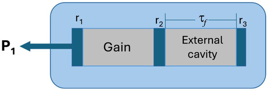
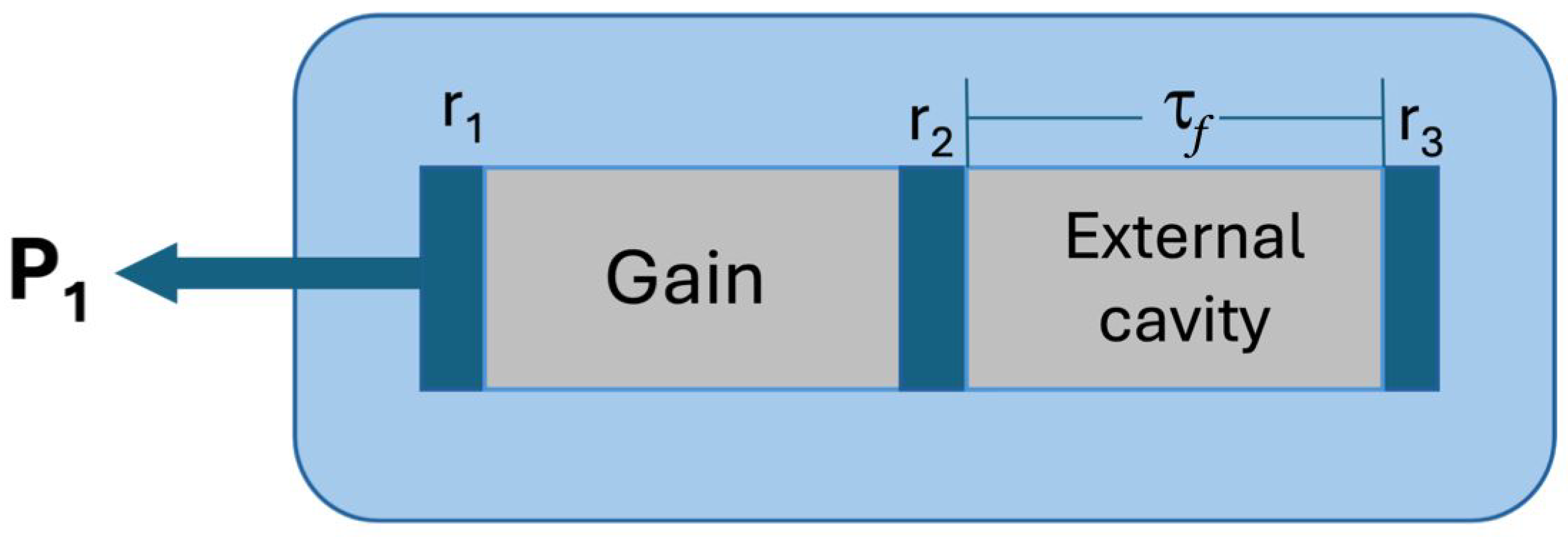
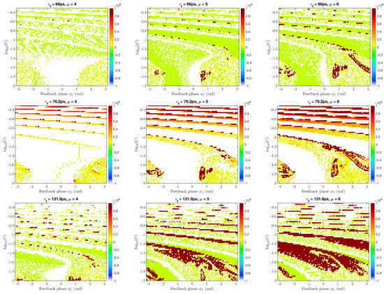
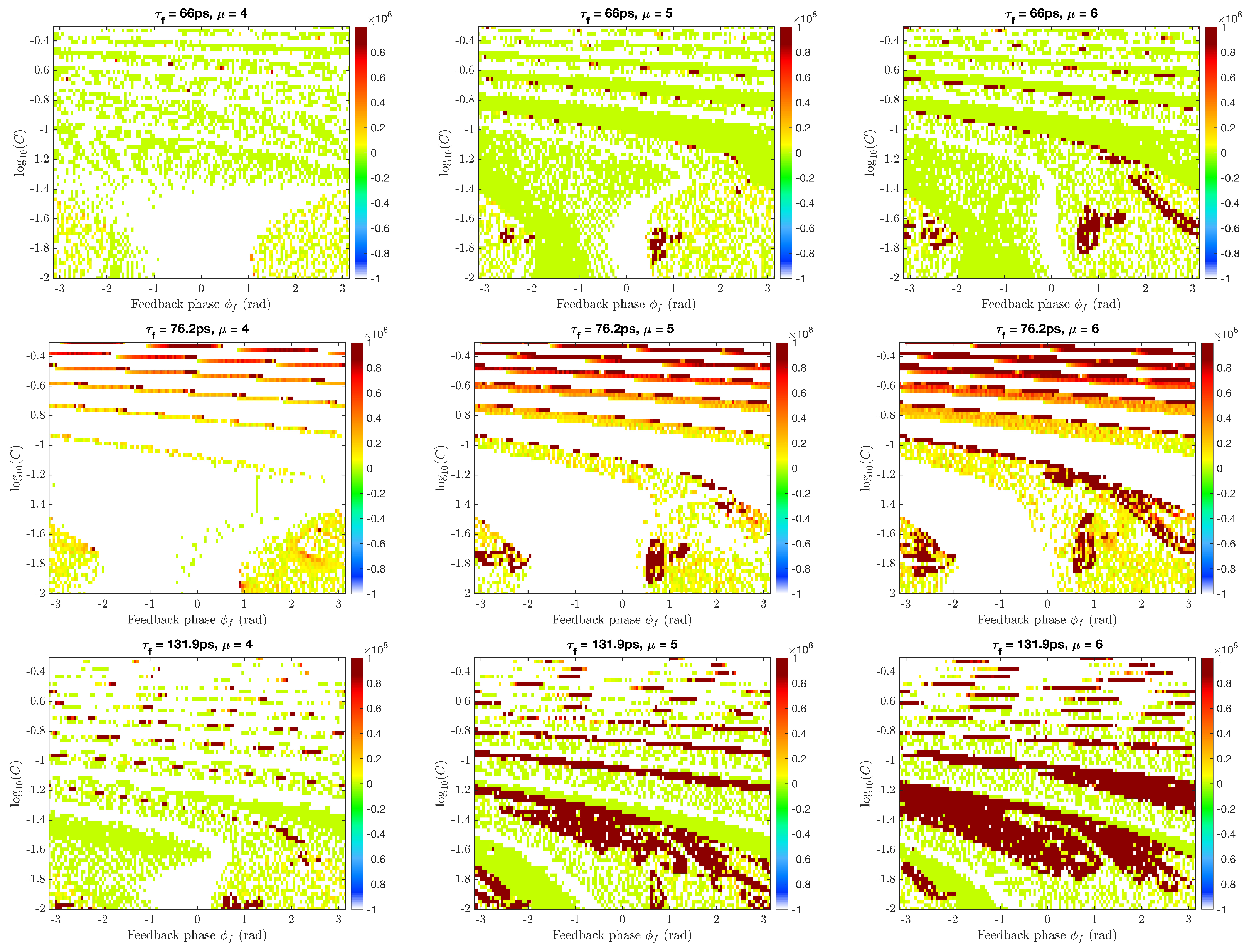
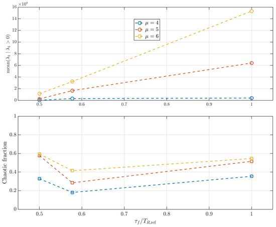
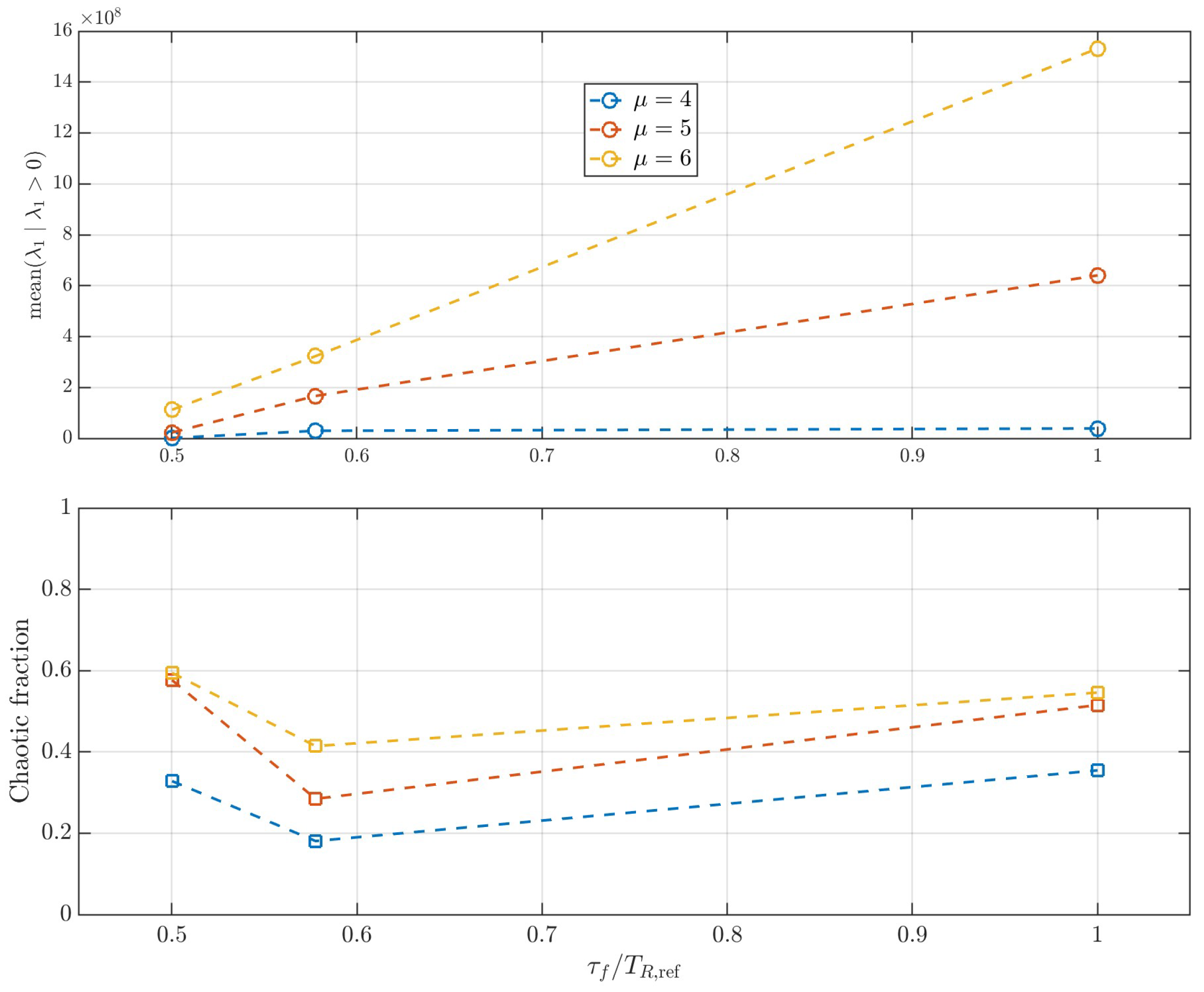
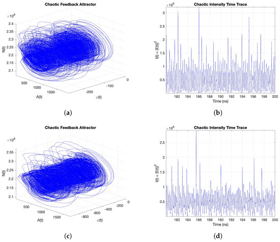

Disclaimer/Publisher’s Note: The statements, opinions and data contained in all publications are solely those of the individual author(s) and contributor(s) and not of MDPI and/or the editor(s). MDPI and/or the editor(s) disclaim responsibility for any injury to people or property resulting from any ideas, methods, instructions or products referred to in the content. |
© 2026 by the authors. Licensee MDPI, Basel, Switzerland. This article is an open access article distributed under the terms and conditions of the Creative Commons Attribution (CC BY) license.