


Abstract
With the rapid growth of urban motorization, personalized travel modes, including taxis and private cars, have expanded considerably. However, conventional public transportation systems, constrained by fixed routes and limited service flexibility, often struggle to satisfy residents’ increasingly diversified and high-quality commuting needs. To address this issue, this study proposes an integrated planning framework for customized bus services using taxi trajectory data. First, passenger origin–destination (OD) information is extracted by detecting changes in the taxi passenger-status field. The extracted OD records are then used to identify potential commuting demand by jointly considering peak-hour travel characteristics and regional OD stability. Second, the identified potential commuting demand is used to generate candidate boarding and alighting stops through an improved DBSCAN-based clustering method, namely IDK-SG. For route planning among the candidate stops, a bi-objective optimization model is developed to simultaneously account for passenger travel-time costs and bus operating costs, and the model is solved using a genetic algorithm. Finally, timetable optimization is formulated as a Markov decision process and solved using a Deep Q-Network (DQN) algorithm. Case studies using taxi GPS trajectory data from Chongqing demonstrate that the proposed framework can effectively identify stable commuting demand, optimize stop layouts and route schemes, and improve vehicle occupancy and service quality. These findings provide practical decision-making support for the operation and dynamic scheduling of customized bus services in urban peak-hour commuting corridors.
1. Introduction
With rapid economic development and the continuous increase in motorization levels, urban transportation systems are facing increasingly severe challenges, including traffic congestion, environmental pollution, energy consumption, and declining travel efficiency [1]. The rapid expansion of personalized travel modes such as taxis, private cars, and ride-hailing services, while enhancing travel flexibility, has also further exacerbated the road resource tightness and the supply demand imbalance during peak hours. In contrast, public transportation has inherent advantages in resource conservation, low-carbon environmental protection, and large-scale collective transport. However, conventional bus services follow fixed operation patterns, making it difficult to respond flexibly to the differentiated spatiotemporal travel demands of residents [2]. Especially during peak commuting hours, conventional buses often suffer from long walking distances, inconvenient transfers, and low on-time arrival rates, which may cause part of the commuting demand to shift from public transportation to taxis and private cars. Therefore, improving service flexibility and travel experience while maintaining the intensification of public transportation has become an important issue in the optimization of urban public transport systems.
Customized bus services [3], as an emerging form of demand-responsive public transportation, provide a feasible solution to the above problems. Customized buses are typically designed to offer faster, more comfortable, and more targeted services for passenger groups with similar spatiotemporal travel characteristics, thereby achieving a more flexible balance between conventional bus services and individualized travel modes. Compared with regular buses, customized buses can improve operational efficiency and punctuality by reducing intermediate stops, optimizing routes and adjusting departure intervals [4]. Compared with taxis and private cars, customized buses provide higher passenger-carrying capacity and lower unit operating costs, enabling them to attract peak-hour commuting demand back to public transportation. Therefore, customized buses can serve as an important supplement for alleviating urban commuting congestion, enhancing the attractiveness of public transportation, and promoting the development of green mobility.
In urban commuting scenarios, customized bus planning needs to address two fundamental questions: “which demands are worth serving” and “how to organize the services”. The former requires identifying potential passenger groups with stable commuting patterns and significant spatiotemporal clustering characteristics from complex travel data. The latter involves interrelated planning decisions, and issues including stop layout, route planning, and timetable optimization. Specifically, stop layout affects passenger walking accessibility, route planning impacts operational efficiency and costs, and timetable optimization directly determines passenger waiting experience and bus utilization. These planning components are strongly interdependent and should therefore be considered within an integrated framework.
In recent years, with the development of traffic sensing and data acquisition technologies, taxi GPS data, which are characterized by high sampling frequency, fine spatial accuracy, and explicit passenger states, have been widely used to identify potential demand for customized buses services. Previous studies have examined customized bus demand mining, stop selection, route planning, and timetable optimization from different perspectives. However, most existing studies focus on optimizing a single or partial aspects of customized bus planning under given demand conditions. Less attention has been paid to how to systematically transform stable commuting demand identified from taxi trajectory data into subsequent decisions on stop selection, route planning, and timetable optimization. Therefore, this study develops an integrated planning framework that transforms taxi trajectory data into customized bus demand, candidate stops, routes planning, and departure schedules. The main novelty of this study lies in the problem-oriented connection of these planning stages, rather than the isolated use of a single algorithm.
The main contributions of this paper can be summarized as follows:
- (1)
- A taxi-trajectory-based method is developed to identify stable commuting demand. Traffic-zone OD pairs with high flow intensity and low inter-day fluctuation are identified, and the corresponding individual OD records are extracted as potential customized bus demand.
- (2)
- A coordinated stop and route planning procedure for customized buses is proposed. Specifically, an improved DBSCAN-based stop selection method (IDK-SG) is developed to extract candidate boarding and alighting stops. On this basis, a bi-objective route planning model that considers both passenger travel-time costs and bus operating costs is constructed and solved using a genetic algorithm.
- (3)
- Timetable optimization is formulated as a Markov decision process, employing the DQN to optimize dispatch intervals, improving vehicle utilization and service quality.
- (4)
- A case study based on taxi GPS data from the main urban area of Chongqing is conducted to verify the effectiveness and application value of the proposed methods in travel demand identification, stop-route layout, and timetable scheduling.
The remainder of this paper is organized as follows. Section 2 reviews the related studies on customized buses. Section 3 introduces the method for identifying stable commuting demand and presents the IDK-SG method for extracting candidate stops. Section 4 constructs the customized buses route planning model and explains the corresponding solution strategy. Section 5 establishes the timetable optimization model and introduces the DQN dynamic solution method. Section 6 presents the case study and the results based on taxi GPS data from the main urban area of Chongqing. Finally, Section 7 concludes the paper and outlines directions for future research.
2. Literature Review
According to the research scope of this study, the relevant literature is summarized as follows.
2.1. Demand Identification
Early studies mainly relied on questionnaires or passenger reservation records to obtain demand information [1,2]. These methods can directly capture passengers’ origins and destinations, departure times, and travel intentions, but they usually suffer from limited sample size, high acquisition costs, and insufficient coverage. With advances in traffic sensing technologies, an increasing number of studies have used multi-source data, including public transport smart card data, mobile phone signaling data, taxi GPS trajectories, and private-vehicle electronic identification data, to identify potential demand for customized bus services.
Existing research indicates that different data sources are suitable for different scenarios. Toole et al. [5] combined mobile phone signaling data, geolocation information, and questionnaire surveys to estimate residents’ travel OD. Yu et al. [6] studied taxi trajectory graph construction. Wang and Chen [7] used taxi order data to identify potential demand scenarios for customized buses from the perspectives of stability and travel frequency, providing a basis for route planning. Xia et al. [8] utilized private-car electronic identification data to extract commuting demand, demonstrated that high frequency and spatiotemporal clustering are key criteria for identifying customized bus demand. Melo et al. [9] developed a demand-responsive transport analysis framework integrating mobile data, operator demand information, and public transport data. Li et al. [10] further regarded the identification of potential customized bus passengers from private-car trajectory data as a trajectory classification problem.
Although the application of multi-source data has provided more possibilities for customized bus research, several limitations remain. Public transport smart card data can only record travel information from existing regular bus passengers and thus cannot capture potential commuting demand currently served by taxi or private cars. Mobile phone signaling data can provide relatively comprehensive trajectory information, but may also raise privacy concerns [9]. In addition, the relationship between different data sources and customized bus demand is often not a direct mapping; further screening and transformation are required by integrating travel stability, commuting characteristics, and spatial clustering features [8,10,11]. Therefore, how to identify potential passenger groups with stable commuting attributes from real trajectory data and integrate them naturally into subsequent bus planning stages remains worthy of further research.
2.2. Stop Selection and Route Planning
Stop selection and route planning are core components of customized bus scheme design and crucial links connecting passenger demand with actual operational services. For stop selection, commonly used methods include K-means, hierarchical clustering, DBSCAN, and their improved variants [12,13,14,15]. Yuan et al. [15] developed a customized buses stop location model by analyzing the passenger-to-stop distance and the bus operating costs, and proposed a dual-population adaptive immune algorithm to solve it. Tian et al. [16] designed a novel customized buses service model to address the impact of large-scale events on the transportation system, in which customized bus stops were determined using graph semi-supervised learning and ensemble algorithms, effectively alleviating the traffic congestion. Overall, previous stop-planning studies have provided the methodological basis for clustering demand points into serviceable boarding and alighting stops.
Customized bus route planning is usually regarded as a vehicle routing optimization problem with time windows, capacity constraints, and multi-objective requirements [17,18,19]. Ma et al. [17] proposed a clustering algorithm based on vehicle trajectory data that automatically extract potential customized bus routes from each cluster, thereby improving the accuracy and efficiency of route planning. Focusing on passengers’ psychological expectations of arrival times and tolerance for delays. Zhen et al. [20] formulated customized on-demand bus routing as a variant of the vehicle routing problem, considering walking limits, time-window requirements and vehicle capacities. Asghari et al. [21] used extensive computational experiments to quantify carpooling behavior in customized bus route planning and verified the effectiveness and applicability of their proposed methods through real-world cases. Chen et al. [22] examined how passenger optimism affects customized bus route selection and generated route operation schemes under different passenger optimism coefficients.
Overall, existing studies have developed relatively rich methodologies for stop selection and route planning. However, two main limitations remain. First, stop selection and route planning are still treated as separate steps in many studies, and the results of stop layouts may not fully match the subsequent route planning. Second, some studies focus mainly on static planning and fail to adequately consider actual demand fluctuations [17,23,24]. Therefore, achieving coordinated stop–route planning while balancing passenger benefits and operator benefits remains an issue worthy of further investigation.
2.3. Timetable Optimization
Most studies on bus timetable optimization consider factors such as departure frequency, travel costs, and passenger demand to construct mathematical models and employ different methods to solve them. Gkiotsalitis and Alesiani [23] generated robust timetables under passenger demand and travel-time uncertainty. Liu Y et al. [25] focused on the dynamic departure problem for a single bus line. They built a robust optimization model aimed at reducing total passenger waiting time. Dou et al. [26] proposed a multi-objective timetable coordination method considering travel time uncertainty, which reduced transfer waiting time and its variability. Liu T et al. [27] further integrated timetable coordination and vehicle scheduling into a model. This approach co-optimizes operating costs and service levels while ensuring balanced headways.
With the rapid development of computers and artificial intelligence, deep reinforcement learning has increasingly been applied to bus scheduling optimization. Yan et al. [28] modeled the multi-route bus timetable optimization problem as a Markov decision process and proposed a multi-agent reinforcement learning algorithm, enabling the model to learn under dynamically changing passenger demand and traffic conditions. Ai et al. [29] treated bus timetable optimization as a sequential decision problem and used reinforcement learning to determine departure intervals. Wang and Sun [30] developed a distributional multi-agent reinforcement learning framework for robust bus holding control under traffic perturbations, service interruptions, and demand surges, while Xia et al. [24] proposed a data-driven distributionally robust model to jointly optimize timetables and dynamic capacity allocation for automated modular bus systems under time-dependent demand uncertainty.
Traditional bus timetables are mostly manually developed by experts based on passenger flow data, resulting in fixed departure schedules. This approach is limited by subjective experience and lacks flexibility. Most existing studies employ heuristic algorithms, such as particle swarm optimization and simulated annealing. However, these methods often seek local optima for a single problem. As a result, they show limited adaptability in complex and dynamic traffic scenarios and cannot achieve real-time timetable optimization or dynamic updating. Therefore, with the development of big data and artificial intelligence, customized bus timetable optimization methods need to be further improved to fully reflect the flexibility and efficiency of customized bus services.
With the development of intelligent and connected vehicle technologies, autonomous vehicles and autonomous shuttle buses have also been discussed as potential carriers for flexible and demand-responsive public transport services. Their application may further reduce operating labor costs and improve the flexibility of route organization, especially in low-density or dynamically changing demand scenarios. However, their practical application depends not only on route-planning and scheduling technologies, but also on passengers’ willingness to accept and use such services. Song et al. [31] assessed public acceptance of autonomous vehicles using a novel IRN PIPRECIA–IRN AROMAN model and showed that acceptance is affected by factors such as attitude, behavioral control, relative advantage, subjective norms, compatibility, hedonic motivation, and complexity. Therefore, future customized bus planning should also consider the interaction between operational optimization and user acceptance when autonomous vehicles are introduced into public transport services.
3. Demand Identification and Stop Selection
Taxi trajectories and trajectory-derived OD information have been widely used for urban travel demand identification, trip-relation modeling, and potential passenger mining for customized bus services [5,6,10,11]. Building on these studies, this paper further focuses on the planning needs of urban commuting customized bus services by screening stable traffic-zone OD pairs with high frequency and low fluctuation from taxi OD records, and then using the selected demand as input for stop selection, route planning, and timetable optimization.
3.1. Method for Identification Stable Commuting Demand
3.1.1. OD Extraction
The original taxi data include a passenger-status field. By analyzing changes in this field, the OD locations of passenger trips can be extracted. The passenger-status field indicates whether a taxi is carrying a passenger, with values of 0 and 1. Therefore, changes in the passenger-status field can be used to infer the origin and destination of each passenger trip.
3.1.2. Traffic Zone Division and Stability Assessment
For customized bus services, suitable travel demand should be relatively stable in both time and space. Therefore, it is necessary to identify stable spatiotemporal components in the OD data, namely commuting components.
- Spatial Characteristics: Commuter trips usually occur repeatedly between relatively fixed functional areas and exhibit strong spatial clustering.
- Temporal Characteristics: Commuter trips are usually concentrated in relatively fixed periods and show clear temporal regularity.
Based on this understanding, this paper does not directly judge commuting behavior at the level of individual boarding and alighting points. Instead, discrete OD records are aggregated to the regional scale through traffic-zone division [5,6,11]. This paper uses passenger flow “frequency” and “stability” as screening criteria. Frequency is measured by the average daily passenger flow between traffic zones, while stability is measured by the coefficient of dispersion (COD). When a traffic-zone pair belongs to a cluster with relatively high average flow and low dispersion, and its travel distance falls within the predefined commuting distance range of 6–30 km, it is regarded as a stable commuting zone pair.
Let the OD flow from traffic zone i to j on the t-th workday be denoted as . The average flow over workdays is defined as
where T is the number of workdays.
To characterize passenger-flow fluctuations for a traffic-zone pair over workdays, the standard deviation is defined as
Then, the traffic-flow dispersion coefficient is introduced to measure passenger-flow stability:
This paper adopts COD = 0.3 as the criterion for passenger-flow stability. This index reflects the relative fluctuation level of passenger flow. A larger indicates stronger fluctuation, suggesting that the demand is more likely to be occasional or unstable. When the average flow is high and the fluctuation is small, the is low, indicating that the traffic-zone pair better conforms to the logic of a “stable commuting relationship”.
Stable commuting demand is identified by jointly analyzing the mean flow and its dispersion coefficient. Since and have different dimensions, direct clustering may be affected by scale differences. Therefore, standardization is first required. This paper adopts the z-score standardization method to convert the two indicators into dimensionless variables. After standardization, and are jointly used as input features for the K-means clustering algorithm to identify commuting traffic-zone pairs.
3.2. Stop Selection Method
Based on the set of identified stable commuting demand points, nearby demand points are aggregated into a limited number of candidate stops, thereby completing customized bus stop selection. This paper mainly studies a “many-to-many” customized bus service model in which stops serve multiple origins and destinations to improve the passenger load factor of customized buses.
Model Construction: Passenger walking distance is a significant factor influencing the choice of customized bus services [15,16]. Therefore, this paper analyzes passenger walking distance and stop service coverage to construct a customized bus stop selection model.
Let the relative coordinates of taxi demand points i (i = 1, 2,…, N) be denoted as (, ), and the relative coordinates of customized buses stops j (j = 1, 2,…, M) be denoted as (, ). The customized bus stop selection model is established as follows:
where N represents the total number of demand points. M represents the total number of candidate bus stops. R represents the coverage radius of stop j. is the decision indicator. = 1 indicates that stop j is selected as a candidate stop, and = 0 otherwise. is the assignment variable, which is 1 if demand point i is assigned to stop j, and 0 otherwise. represents the distance from demand point i to candidate customized bus stop j. Therefore, the specific expression of the customized bus stop selection model is:
This shows that the stop selection problem is essentially a demand clustering and center extraction problem under service-radius constraints. Considering that stable commuting demand points exhibit clear spatial clustering and may contain a small number of discrete noise points, this paper proposes an improved DBSCAN-based stop selection method, namely IDK-SG. This method first uses DBSCAN to identify valid clusters and remove noise points based on the density-reachability relationship among demand points. K-means is then applied to extract cluster centers from the denoised demand points, thereby generating stops with strong interpretability and operability.
The main steps of the IDK-SG algorithm are as follows:
Step 1: Input the stable commuting demand point dataset P. A demand point is denoted as . Where represents the spatial coordinates of the i-th demand point, all demand points constitute the original sample set P.
Step 2: Initialize the cluster counter k = 0, and set the candidate parameter range for the DBSCAN clustering algorithm, including the neighborhood radius Eps and the minimum sample number threshold MinPts. For any two demand points, and , their spatial distance is defined as
When < Eps, is considered to fall within the spatial neighborhood of . If the number of samples in the neighborhood of a point is not less than MinPts, it is regarded as a core point.
Step 3: Perform DBSCAN clustering under different parameter combinations (Eps, MinPts) to initially identify demand-point clusters. For each parameter combination, the silhouette coefficient is used to evaluate clustering performance. Let the silhouette coefficient of sample i be
where represents the average distance between sample i and other samples in the same cluster, and represents the average distance between sample i and sample in the nearest neighboring cluster. The optimal DBSCAN parameters are determined by comparing the overall silhouette coefficients under different parameter combinations.
Step 4: Re-execute DBSCAN under the optimal parameter combination and remove all points identified as noise. Let the remaining demand points form a new dataset A, where a point in A is denoted as . This dataset serves as the input for subsequent K-means center extraction.
Step 5: Use K-means to extract the centers from the denoised demand point dataset A. Let the number of cluster centers be K, and the initial cluster centers be denoted as . The distance from any demand point to cluster center is denoted as . Each demand point is assigned to the nearest cluster center.
Step 6: Iteratively update each cluster center and repeat the sample assignment. The sum of squared errors (SSE) is used to evaluate the current clustering result. When the change in SSE between two consecutive iterations is smaller than a given precision threshold, the clustering result is considered converged.
Step 7: Adjust the number of clusters K, repeat Steps 5–6, and use the SSE to evaluate the clustering effects under different K values. The result that satisfies the stop layout constraints and demonstrates the best clustering effectiveness is selected as the candidate boarding and alighting stops for customized bus services.
In summary, through a two-stage procedure, the IDK-SG method transforms stable commuting demand points into a set of serviceable candidate stops, providing a basis for subsequent route planning.
4. Customized Bus Route Planning Model
Based on the passenger demand at each candidate stop, the route planning is modeled as a vehicle routing problem with capacity, stop-service, and maximum-route-length constraints [17,19]. The model aims to minimize bus operating cost while satisfying all passenger travel demand and maintaining an acceptable passenger travel-time level.
4.1. Route Planning Model Formulation
4.1.1. Objective Function
- 1.
- Passenger Travel-Time Cost: Passenger travel time consists of three components—in-vehicle travel time between stops, walking time from the origin to the boarding stop, and walking time from the alighting stop to the destination. The objective function for passenger travel-time cost is shown in Equation (10).where P is the set of travel nodes, Q is the set of passenger travel demands, and K is the set of vehicles. If bus k travels from stop i to stop j, then = 1, otherwise, = 0. represents the passenger demand served by bus k from stop i to stop j, represents the actual distance between stop i and stop j, represents the average passenger walking distance, represents the average vehicle speed, represents the average passenger walking speed, and γ is the passenger time value coefficient.
- 2.
- Bus Operating Costs: Customized buses’ operating costs include per-kilometer operating costs, such as energy consumption costs, and fixed operating costs, such as driver wages and vehicle depreciation. The bus operating cost objective is given in Equation (11).where represents the fixed operating cost of bus k, and represents the per-kilometer operating cost of bus k.
Finally, the comprehensive optimization objective is obtained by linearly weighting passenger travel-time cost and bus operating cost, as shown in Equation (12). The linear weighted structure follows the common treatment of multi-objective optimization problems [20]. In the case study, equal weights are adopted after normalization to avoid dominance caused by different units.
4.1.2. Constraints
- 1.
- Stop Access Constraint: Each customized bus stop should be accessed at least once, and the same vehicle is not allowed to access the same stop more than once during a single trip. The stop access constraint is shown as follows:where D is the set of alighting stops.
- 2.
- Vehicle Load Factor Constraint. To improve operational efficiency, customized bus routes should satisfy a minimum vehicle load factor. Specifically, the ratio of the actual passenger count to the maximum capacity for a single trip of bus k must satisfy the minimum-load-factor constraint.
- 3.
- Stop number constraint. To guarantee service quality, customized bus services impose a strict constraint on the number of stops served within a single trip. This is a significant difference between customized buses and conventional buses.where A represents the set of boarding stops. If bus k stops at stop i, then = 1, otherwise, = 0.
- 4.
- Maximum Route Length Constraint. Excessively long customized bus routes increase passenger travel time and reduce passenger travel experience. Therefore, the length of each customized bus route should be limited.
4.2. Model Optimization and Solution
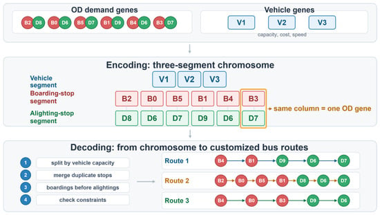
The customized bus route planning problem involves vehicle assignment, ordered boarding and alighting stop sequences, and multiple operational constraints, leading to strong discreteness and combinatorial complexity. Given the population-based search and global optimization capability of genetic algorithms for complex optimization problems [32,33], this study adopts a GA as the solution framework for the route planning model. Based on the service characteristics of many-to-many customized bus services, the chromosome is organized into a vehicle segment, a boarding-stop sequence, and an alighting-stop sequence. A decoding procedure is used to transform each individual into feasible multi-route schemes under capacity, load factor, stop coverage, and route length constraints.
- Chromosome Representation: This paper adopts a “three-stage independent encoding” strategy to divide the chromosome into three sequences. Segment 1 is the vehicle segment, in which each gene denotes the vehicle assigned to a route and records the corresponding capacity, fixed cost, per-kilometer operating cost, and speed. Segment 2 is the boarding-stop sequence, and Segment 3 is the alighting-stop sequence. The two stop sequences have the same length and are paired by position. During decoding, the ordered OD-demand list is allocated to available vehicles according to vehicle capacity and feasibility constraints. For each vehicle, duplicated boarding or alighting stop identifiers are merged, boarding stops are placed before alighting stops, and the resulting stop sequence is evaluated as one candidate customized bus route. The encoding and decoding process is shown in Figure 1.Figure 1. Chromosome encoding and decoding logic. Blue, red, and green blocks denote vehicle genes, boarding-stop genes, and alighting-stop genes, respectively; arrows indicate the encoding and decoding flow from OD-demand genes to vehicle-specific customized bus routes.
- Fitness Function. Each chromosome is first decoded into a complete multi-route scheme and checked against the stop-coverage, vehicle-capacity, minimum-load-factor, stop-number, and maximum-route-length constraints. Infeasible individuals are assigned penalty values to reduce their probability of being selected. For feasible individuals, the fitness value is calculated directly from the comprehensive objective function in Equation (12), namely the weighted sum of passenger travel-time cost and bus operating cost. Since the proposed model is a minimization problem, a smaller comprehensive objective value indicates a better route scheme in terms of the trade-off between passenger service level and operating cost.
- Genetic Operations:
- Selection: The tournament method is used for selection. First, the number of individuals compared in each round is set as N. Then, N individuals are randomly selected from the population, their fitness values are calculated and compared, and the best individual is added to the next generation.
- Crossover: The order crossover (OX) method is adopted to ensure that each gene appears exactly once in each chromosome. A contiguous segment is randomly selected, and the genes within this segment from parent A are copied to the corresponding positions in the offspring. Then, the remaining genes from parent B that are not included in the selected segment are then sequentially filled into the empty positions of the offspring. To maintain the OD-demand correspondence, the same crossover positions are applied synchronously to the boarding and alighting sequences. The vehicle segment is exchanged between the two parents by route unit so that useful vehicle-assignment information can also be inherited.
- Mutation: Mutation is used to increase population diversity and reduce the risk of premature convergence. In this study, two mutation strategies are applied with a predefined mutation probability. The first changes a vehicle-type or vehicle-assignment gene in the vehicle segment to adjust the matching relationship between vehicles and routes. The second randomly selects two positions in the stop-demand sequence and swaps the boarding genes together with their corresponding alighting genes, thereby preserving the OD-demand pairing. The mutated chromosome is then decoded and evaluated again. If the resulting route scheme violates capacity, load-factor, stop-coverage, or route-length constraints, it is handled by the penalty mechanism; otherwise, it enters the subsequent selection process.
- Termination Condition: The algorithm terminates when the maximum number of iterations is reached or when the variation in consecutive optimal solutions falls below a predefined threshold.
5. DQN-Based Timetable Optimization Model
5.1. Problem Description
Customized bus timetable optimization is a typical sequential decision-making problem, because each departure decision affects subsequent passenger waiting time, vehicle utilization, and operating cost. Following the Markov decision process (MDP) framework, the service period is discretized into consecutive 1 min decision epochs, and the departure process is described by states, actions, state transitions, and rewards [34,35]. Based on this formulation, a Deep Q-Network (DQN) is adopted to solve the MDP. DQN approximates the action-value function using a deep neural network and is suitable for dynamic decision-making problems with complex state spaces [36].
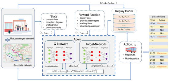
In the model of this paper, the state variables are constructed from service time, waiting demand, vehicle loading status, and passenger waiting information. The action space contains two discrete actions, namely departure and non-departure, subject to minimum and maximum headway constraints. The reward function jointly considers load utilization, departure cost, passenger waiting time, and stranded-passenger penalties. In this way, the DQN is used to learn a departure policy that dynamically adjusts headways according to time-varying passenger demand. The detailed network architecture and training parameters are reported in the case-study section. To clearly illustrate the relationships among state observation, action selection, reward feedback, and policy updating in customized bus timetable optimization, the DQN-based departure-scheduling optimization framework is constructed, as shown in Figure 2.
Figure 2.
DQN-based customized bus timetable optimization framework. Arrows indicate the information flow in the DQN-based scheduling process. Dots represent neurons in the neural-network modules, and ellipses indicate omitted intermediate records for schematic simplification. Colors are used only to distinguish functional modules or network layers.
5.2. MDP Formulation for Timetable Optimization
This paper formulates customized bus timetable optimization as a Markov decision process (MDP), characterized by a quintuple: <S, A, P, R, γ>. Specifically, S represents the state space, A represents the action space, and P represents the state transition probability matrix, defined in Equation (17). represents the probability of transitioning to state after executing action a in state s. R represents the reward function, defined in Equation (18), where represents the expected reward value at the next time step after executing action a in state s at time t. γ is the discount factor, which controls the trade-off between immediate and future rewards.
- 1.
- Agent: In the context of single-route customized bus timetable optimization, the agent is defined as the dispatching controller of the customized bus route. At each time step, the agent observes and obtains state , selects an action according to the current policy, and then receives reward , and transitions to the next state , as shown in Equation (19):
- 2.
- State Space Design: The state reflects the information observed by the agent from the environment and affects both decision-making and the convergence behavior of the learning algorithm. This study constructs the state space by integrating passenger demand and road network status. To enhance training stability, all state features are normalized to the interval [0, 1]. The comprehensive state space is defined as follows:where represents the time dimension. The agent continuously monitors two critical environmental variables: the real-time count of waiting passengers within the designated boarding zones of, and the bus operational status in the road network. Since agent-environment interaction occurs at discrete 1 min intervals, the temporal dimension of the customized bus service is represented by the current minute index . For example, 15:00 can be represented as the 900th minute of the day. The service duration is predetermined and denoted by . Therefore, state is calculated as follows:
represents the load factor state. If the bus departing at minute m reaches its maximum capacity during operation, passengers waiting at the stop may remain unserved. The maximum bus capacity is defined as , and the maximum passenger load of the bus departing at minute m is denoted as , where < . Therefore, the load factor is calculated as follows:
represents the passenger waiting-time state. The arrival time and boarding time of each passenger are extracted from the environment, where i represents a specific stop in the customized bus boarding area, and N represents the total number of passengers boarding the bus departing at minute m. Let represents the aggregate waiting time of all passengers served by the bus departing at minute m. It is calculated as follows:
represents the passenger capacity utilization state, calculated as , where represents the maximum passenger capacity of the bus, and represents the utilized passenger capacity. The number of passengers on board, (), and the number of passengers boarding, (), when the bus departing at minute m reaches stop i, are obtained from the environment. The utilized passenger capacity for a single departure is calculated as follows:
The passenger capacity provided by the customized bus is defined as the number of available seats across all stops in the boarding area during a single departure, calculated as follows:
Therefore, the passenger utilization rate is calculated as follows:
- 3.
- Action Space Design: At each time step, the agent determines whether to dispatch a bus based on an action space containing two actions, where a = 1 indicates departure and a = 0 indicates no departure. To reduce the exploration space, a maximum departure interval Imax and a minimum departure interval Imin are introduced. The agent dynamically adjusts the departure interval according to passenger demand, while ensuring that the interval remains within the range defined Imax and Imin.
- 4.
- Reward Function Design: The main goal of the customized bus timetable optimization is to meet passenger demand while reducing bus operating costs. Therefore, the reward function comprehensively consider three factors: bus capacity utilization, bus operating costs, and passenger comfort.
- Bus Capacity Utilization Rate: The passenger capacity utilization rate reflects the level of passenger demand in the environment and is denoted as . A higher utilization rate indicates stronger passenger demand, and the agent is more likely to choose the departure action. Therefore, a reward of is assigned to the departure action (a = 1), while a reward of is assigned to the non-departure action (a = 0).
- Bus Operating Cost: Each departure decision incurs bus operating costs. Let represent the cost of one departure. Therefore, a negative reward of is assigned to the departure action (a = 1).
- Passenger Comfort: This study treats passenger comfort as an important optimization objective. Passenger waiting time and in-vehicle congestion are two key factors affecting passenger comfort. Therefore, a negative reward of is assigned to the non-departure action, and a stranded-passenger penalty of is assigned to both departure and non-departure actions.
In summary, the comprehensive reward function is formulated as follows:
where represents the total number of stranded passengers generated at minute m, α represents the passenger waiting time normalization factor, and β represents the stranded-passenger penalty coefficient.
6. Case Study
This study uses full-day GPS trajectory data from 12,162 taxis in the main urban area of Chongqing over five consecutive weekdays. The data were obtained from an anonymized taxi operation data dataset for research purposes. Because the raw GPS trajectories contain sensitive vehicle and trip information and are subject to data-use restrictions, they are not publicly deposited in an online repository. After data processing, 1,201,117 valid OD trip records from 11,722 taxis were extracted and used for the subsequent experiments.
6.1. Stable Commuting Demand Identification Results
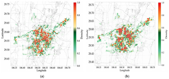
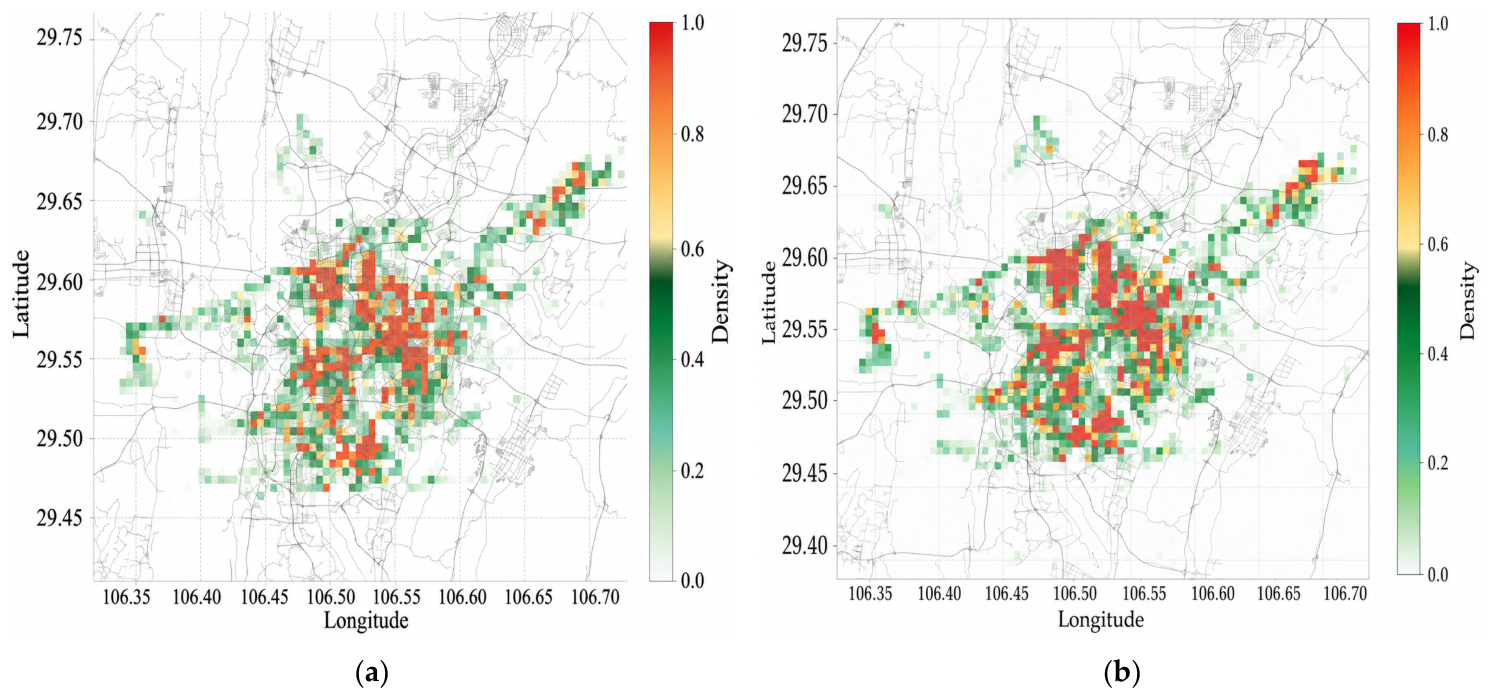
First, the spatial characteristics of taxi OD data in the study area were systematically analyzed to characterize demand hotspots, as shown in Figure 3. As shown in the figure, taxi OD points are relatively concentrated in the core area of the main urban area, mainly in Yuzhong District, Yubei District, Shapingba District, Jiulongpo District, and parts of Nan’an District, indicating strong weekday commuting connections in these areas.
Figure 3.
(a) Spatial distribution heat map of taxi pickup locations; (b) spatial distribution heat map of taxi drop-off locations. The dashed grid lines indicate longitude and latitude reference lines.
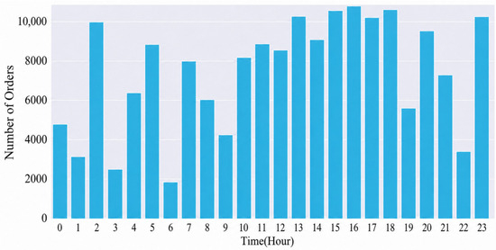
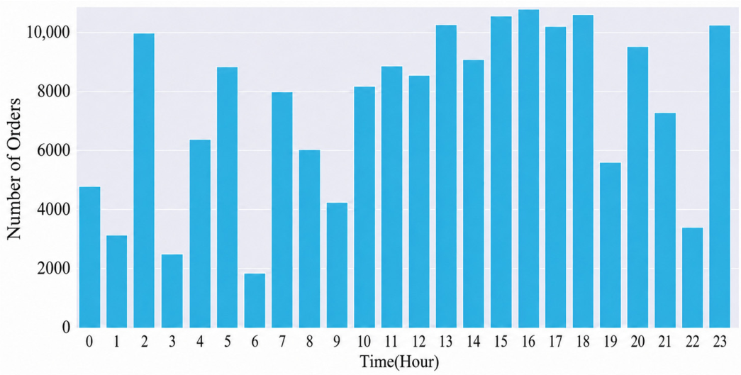
The temporal characteristics of taxi travel demand were analyzed using the hourly order volume shown in Figure 4. It can be seen that taxi orders remained at a relatively high level between 15:00 and 18:00, significantly exceeding those in other periods. Therefore, this period was selected as the evening peak study period to identify potential customized bus demand with stable commuting characteristics.
Figure 4.
Distribution of taxi order volume on weekdays.
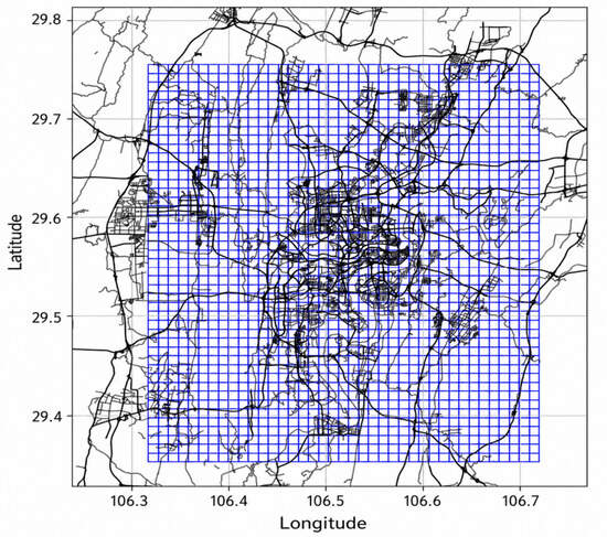
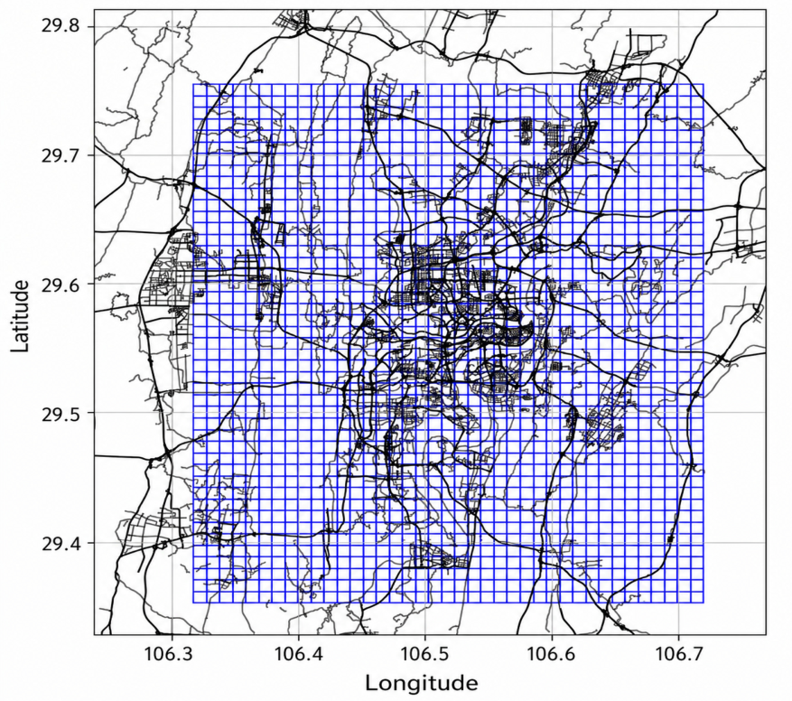
Based on the spatial and temporal analyses, the study area was divided into a uniform grid system with a resolution of 1000 m × 1000 m to construct OD relationships at the traffic-analysis-zone level. Ultimately, the study area was divided into 39 × 45 unit grids, comprising 1755 traffic zones, as shown in Figure 5. By mapping taxi OD data to the corresponding traffic zones, fine-grained order-level trip records were aggregated into regional commuting flows.
Figure 5.
Unit grid division of the study area. The blue grid lines represent the 1000 m × 1000 m traffic-zone units.
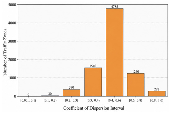
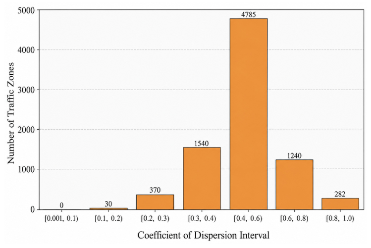
After mapping the taxi OD data to traffic zones, the traffic-zone pairs were sorted by OD volume. Traffic-zone pairs satisfying two criteria, namely relatively high trip volume and travel distances ranging from 6 to 30 km, were selected for subsequent analysis. On this basis, the traffic-flow dispersion coefficients for each traffic-zone pair were calculated. The statistical distribution of the traffic-flow dispersion coefficients is shown in Figure 6. The results show that the dispersion coefficients were mainly distributed within the range of [0.1, 1.0]. Some traffic-zone pairs exhibited both high traffic volume and low fluctuation, indicating typical characteristics of stable commuting demand.
Figure 6.
Statistical distribution of traffic-flow dispersion coefficients.
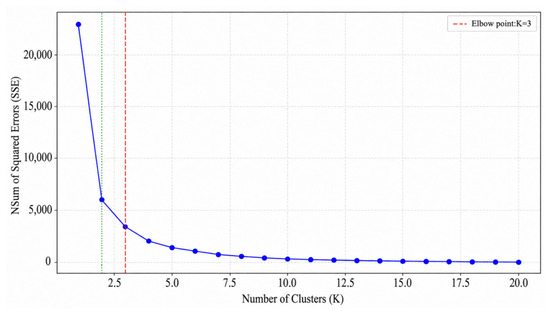
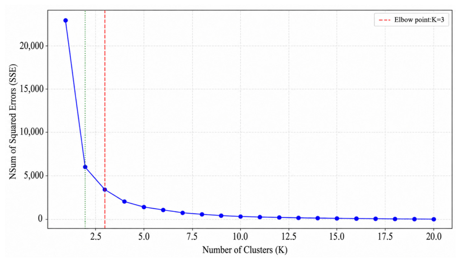
To further identify high-frequency and stable commuting areas, the standardized mean traffic flow and dispersion coefficient of traffic-zone pairs were used as the input features for K-means clustering. The optimal number of clusters was determined by the elbow method, as shown in Figure 7. The plot exhibits a clear inflection point at K = 3. Therefore, the traffic-zone pairs were divided into three clusters, with their detailed characteristics summarized in Table 1. Notably, Cluster 2 has a relatively higher mean traffic flow and a lower dispersion coefficient, indicating that this type of traffic-zone pair simultaneously satisfies the requirements of high passenger volume and strong commuting stability.
Figure 7.
K-means clustering analysis of traffic-zone pairs. The blue curve shows how the sum of squared errors (SSE) changes with the number of clusters; the green dashed line shows the reference spot before the elbow, and the red dashed line marks the chosen elbow point at K = 3.
Table 1.
Traffic zone pair clustering results.
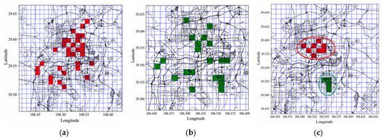
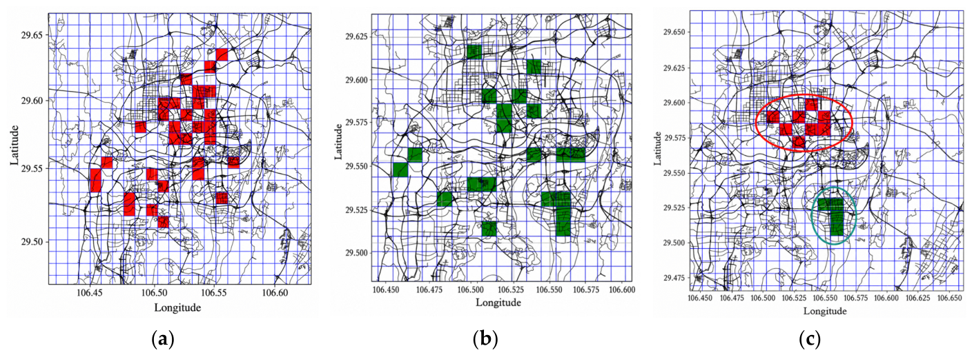
Based on the clustering results, 51 stable commuting zone pairs were identified. These 51 pairs represent traffic-zone-level OD relationships rather than final bus stop pairs. Their origin and destination demand points were further extracted and used as the input for stop clustering. Therefore, the subsequent refinement from stable zone pairs to boarding and alighting stops reflects the transformation from regional OD demand to serviceable stop layouts. The origins, destinations, and final boarding and alighting service areas for customized bus services are shown in Figure 8. It can be seen that the origins of these traffic-zone pairs are mainly concentrated in business and office areas, such as Yubei District and Jiangbei District. The destinations are mainly distributed in residential areas near Nanping in Nan’an District. This reveals a clear evening peak commuting pattern from work areas to residential areas. By combining the density distribution of the traffic-zone pairs with regional functional attributes, the boarding and alighting areas for the customized bus services were finally determined. In Figure 8c, the red area represents the boarding area, and the green area represents the alighting area.
Figure 8.
K-means clustering results of traffic-zone OD pairs when K = 3: (a) origins of traffic-zone OD pairs; (b) destinations of traffic-zone OD pairs; (c) final origin and destination areas for customized bus services. Red and green grid cells indicate origin and destination traffic zones, respectively; blue grid lines represent the traffic-zone division, black lines show the background road network for spatial reference, and the red and green rings in (c) highlight the final boarding and alighting service areas.
6.2. Stop Selection Results
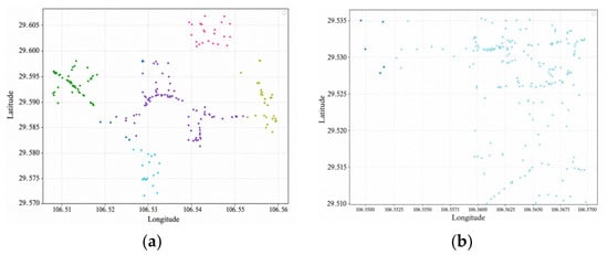
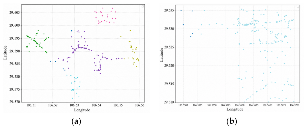
After identifying the stable commuting areas, this study further conducted stop clustering based on stable commuting demand points. First, DBSCAN was implemented separately for boarding and alighting points with a neighborhood radius of Eps = 500 m for preliminary clustering. The clustering results are shown in Figure 9. As shown in the figure, the boarding demand points are mainly concentrated in commercial areas such as Guanyinqiao Business District, Zijin Business Plaza, and Wanhui Center in Jiangbei District, whereas the alighting demand points are mainly distributed in residential areas near Nanping in Nan’an District, with a relatively more dispersed spatial distribution.
Figure 9.
(a) Preliminary clustering result of boarding points with noise; (b) preliminary clustering result of alighting points with noise. Dots with different colors represent different clusters identified by DBSCAN.
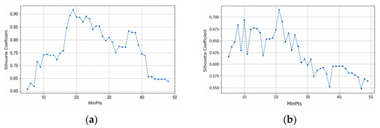
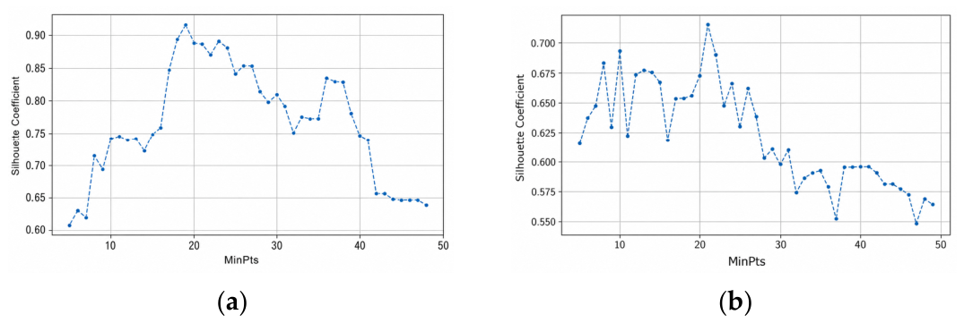
Then, the clustering performance was evaluated under different MinPts values using the silhouette coefficient as the optimization metric. The results are shown in Figure 10. When MinPts = 19 for the boarding points and MinPts = 21 for the alighting points, the silhouette coefficient reaches a relatively optimal level. Therefore, these parameter setting were selected for subsequent stop clustering.
Figure 10.
(a) Clustering results for boarding stops with different MinPts values; (b) clustering results for alighting stops with different MinPts values.
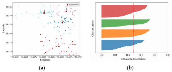
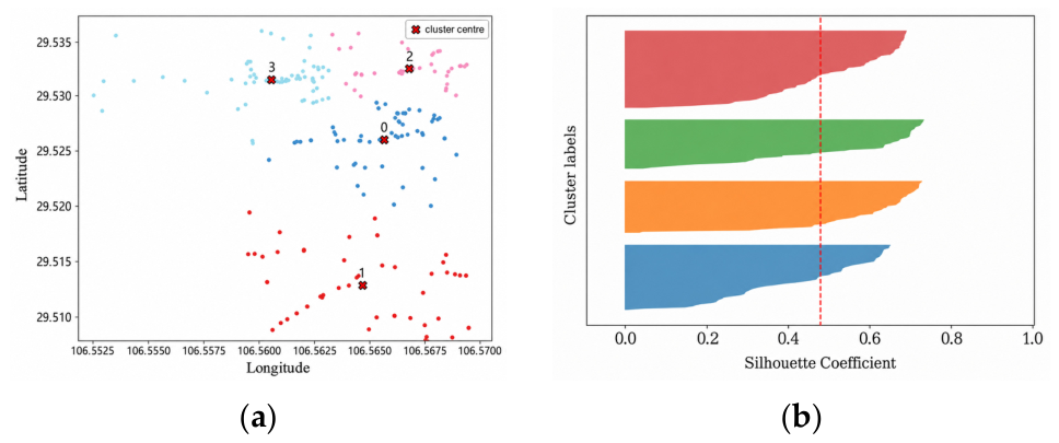
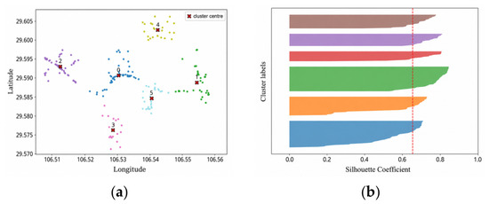
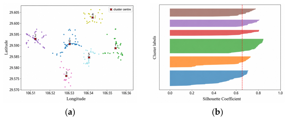
Under the optimal parameter settings, the IDK-SG algorithm was executed, and K-means was further applied to the denoised demand points to extract cluster centers. The clustering performance under different K values was compared separately for boarding and alighting points. The results indicate that the optimal clustering performance was achieved when K = 6 for the boarding points, and K = 4 for the alighting points. The final clustering results and silhouette-coefficient variations for the boarding and alighting points are shown in Figure 11 and Figure 12, respectively. It can be seen that, under these parameter settings, the clusters achieve an excellent balance between intra-cluster compactness and inter-cluster separation, effectively capturing the spatial distribution pattern of stable commuting demand points.
Figure 11.
(a) Clustering results for boarding points; (b) silhouette coefficient results for boarding points. Different colors denote different clusters, numbered markers denote selected candidate stops, and the red dashed line in (b) denotes the average silhouette coefficient.
Figure 12.
(a) Clustering results for alighting points; (b) silhouette coefficient results for alighting points. Different colors denote different clusters, numbered markers denote selected candidate stops, and the red dashed line in (b) denotes the average silhouette coefficient.
Based on the existing of regular bus stop distribution in Chongqing, the proposed candidate stops were refined. If an existing regular bus stop was located within a 500 m radius of a cluster center, the candidate stop was merged with the existing stop to minimize redundant infrastructure and maximize the use of existing bus facilities. Ultimately, six boarding stops and four alighting stops were determined, and their stop IDs, names, types, and construction requirements are summarized in Table 2.
Table 2.
Boarding and alighting stop information.
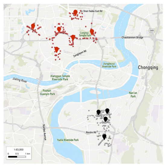
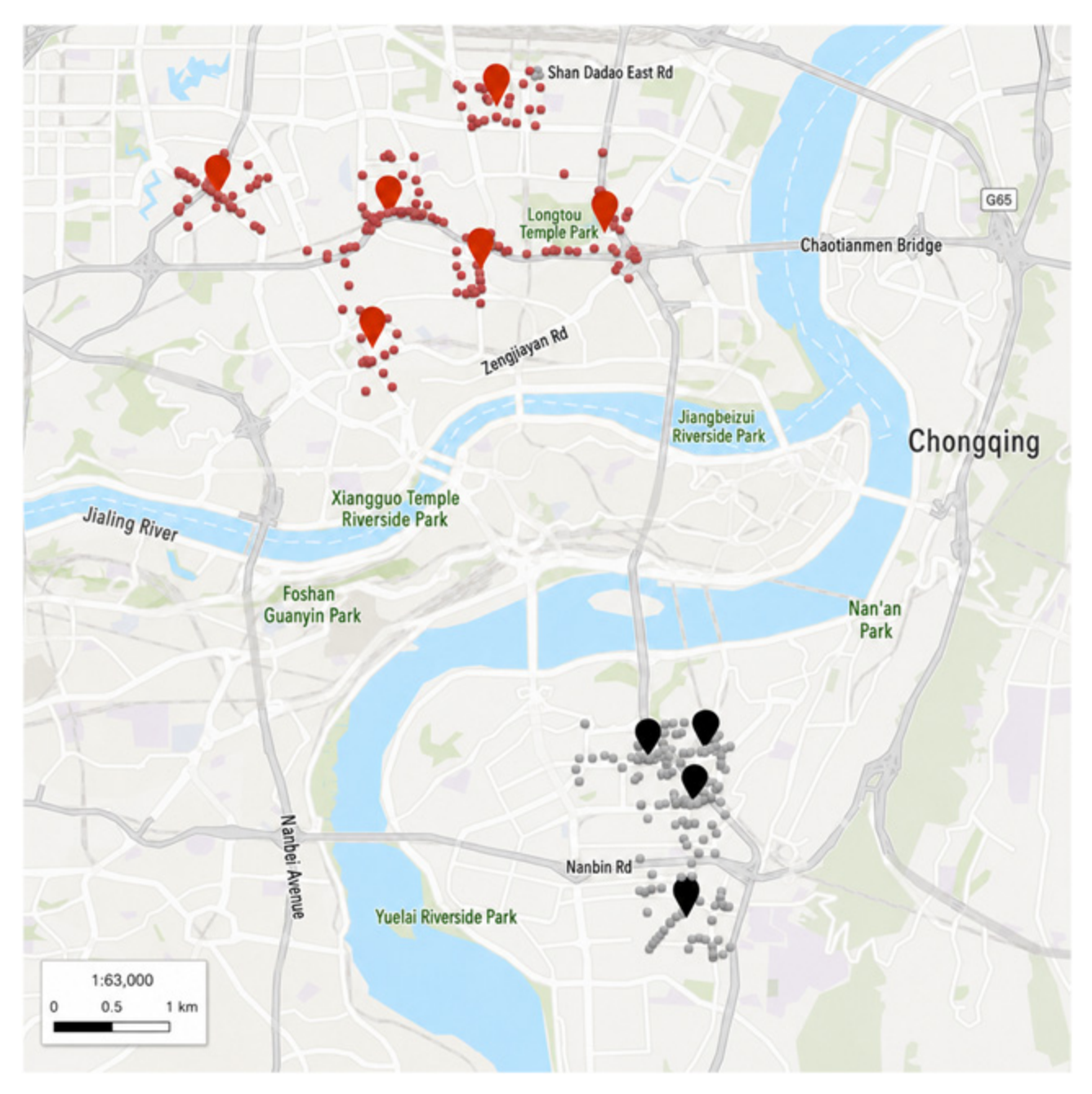
The final distribution of stops and surrounding demand points was shown in Figure 13. The boarding stops are primarily located in commercial districts such as Guanyinqiao, Jianxin East Road, and Wuhong Road, while the alighting stops are mainly distributed in densely populated residential areas such as Nanping, Erxiaoqu, and Sunshine Meidi. Overall, the stop layout aligned well with the spatial distribution of evening peak commuting demand, indicating that the IDK-SG method can effectively transform discrete demand points into feasible candidate stops for customized bus services.
Figure 13.
Distribution of stops and passenger demand in the boarding and alighting areas. Red points indicate boarding stops and their surrounding demand points, while black points indicate alighting stops and their surrounding demand points.
To further verify the effectiveness of the IDK-SG method in customized bus stop selection, it was compared with standalone K-means under the same numbers of boarding and alighting stops. The comparison indicators include mean walking distance, 500 m service coverage, silhouette coefficient, and SSE, and the experimental results are reported in Table 3.
Table 3.
Comparison of stop-selection performance between IDK-SG and K-means.
The results show that compared with the standalone K-means method, the proposed IDK-SG method achieves shorter average walking distance, better clustering validity, and lower SSE values while maintaining the same 500 m service coverage. Specifically, the mean walking distance is reduced from 348 m to 344 m in the boarding area and from 275 m to 268 m in the alighting area. Although the silhouette coefficient is comparable between the two methods, IDK-SG obtains lower SSE values in both areas, indicating a more compact stop layout after removing scattered noise points. These results show that the proposed two-stage clustering procedure can improve stop accessibility and spatial compactness while maintaining the same service coverage.
6.3. Customized Bus Route Planning
Before conducting the customized bus route-planning experiment, the model parameters related to passenger travel-time cost and bus operating cost were specified. The main parameter settings are listed in Table 4.
Table 4.
Algorithm parameters.
In the GA implementation, the initial population size was set to 50, the crossover probability was set to 0.8, the mutation probability was set to 0.2, and the maximum number of iterations was set to 500. These parameters were used to control the population size, genetic operation intensity, and termination condition, thereby balancing computational efficiency and solution quality.
After stop selection, the six boarding stops and four alighting stops were treated as an integrated stop system for route planning, rather than being optimized separately by spatial cluster. The OD matrix among these ten stops was converted into passenger demand genes. In the GA, one chromosome represents a complete multi-route scheme, and the passenger OD demand genes determine the set of boarding and alighting stops assigned to each vehicle. During decoding, the OD demands assigned to the same vehicle are converted into one customized bus route under the vehicle-capacity, load-factor, stop-coverage, and route-length constraints, and duplicated stop identifiers are removed to generate the final stop sequence. Based on the above parameter settings and the GA solution process, the best chromosome was decoded into three customized bus routes. The stop sequences, route lengths, and travel times of the optimized routes are presented in Table 5.
Table 5.
Results of route optimization.
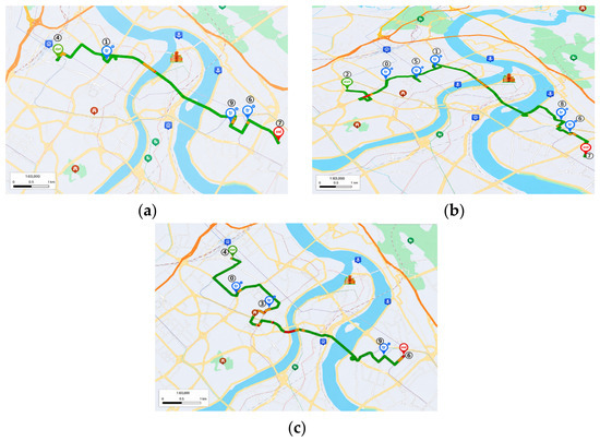
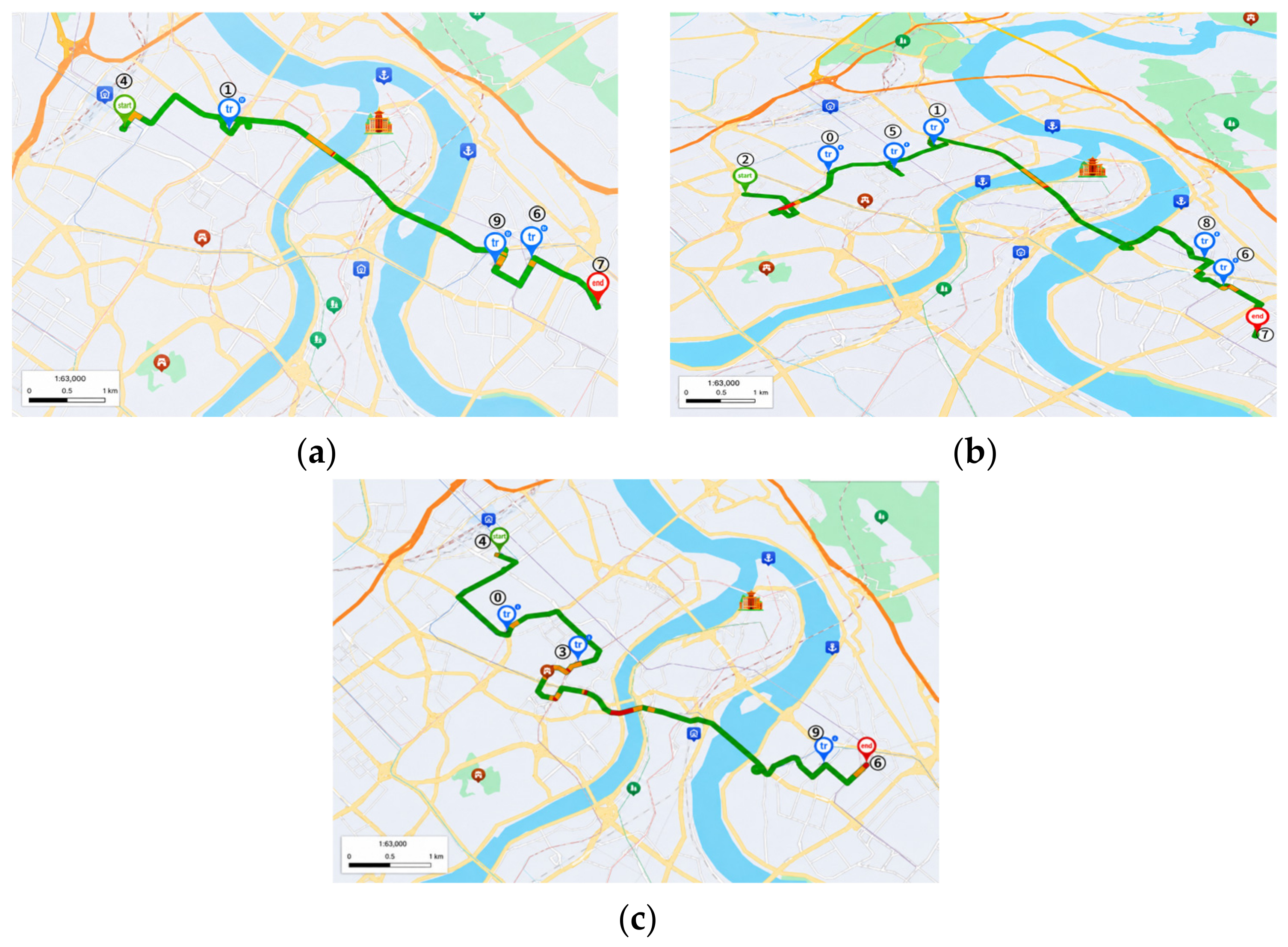
To further illustrate the spatial distribution characteristics of the optimized routes, the operating paths of the three customized bus routes are mapped in Figure 14. This shows that Routes 1 and 3 each contain five stops and mainly serve relatively concentrated commuting demand. Route 2 contains seven stops because the corresponding vehicle is assigned a more dispersed set of OD demands, involving boarding stops 2, 0, 5, and 1 and alighting stops 8, 6, and 7. After decoding, these assigned demands generate the path “2-0-5-1-8-6-7”. Although Route 2 has more stops and a longer travel distance, it still satisfies the maximum route-length and travel-time requirements. This result indicates that the GA reorganizes demand within the whole stop system to balance passenger time cost and operating cost.
Figure 14.
Route maps of customized bus routes: (a) Route 1, (b) Route 2, (c) Route 3.The green lines indicate the optimized travel paths, the numbered markers denote the stop IDs, and the background map colors and icons are used only for spatial reference.
To verify the effectiveness of the proposed GA-based route-planning method, it was compared with a greedy algorithm under the same stop set, OD demand matrix, vehicle capacity, and maximum route-length constraints. The comparison results in terms of route count (RC), total travel distance (TD), mean load factor (MLF), operating cost (OC), passenger time cost (PTC), and overall objective value (OTV) are shown in Table 6.
Table 6.
Comparison of route-planning performance between GA and the greedy algorithm.
The results show that the GA-based method obtains a lower overall target value than the greedy algorithm, decreasing it from 361 to 320. Although the GA solution uses one additional route and has a higher operating cost, it substantially reduces passenger time cost from 448 to 272 and increases the mean load factor from 74% to 85%. This indicates that the GA can search for a more balanced route scheme by jointly considering passenger travel efficiency and vehicle utilization, rather than only pursuing local cost reductions. Therefore, the GA-based route-planning method provides better overall performance for the many-to-many customized bus planning problem.
6.4. Customized Bus Timetable Optimization
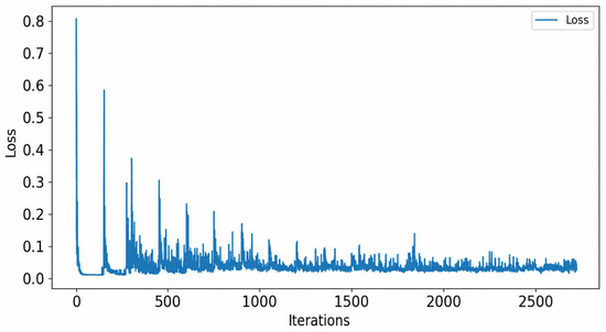
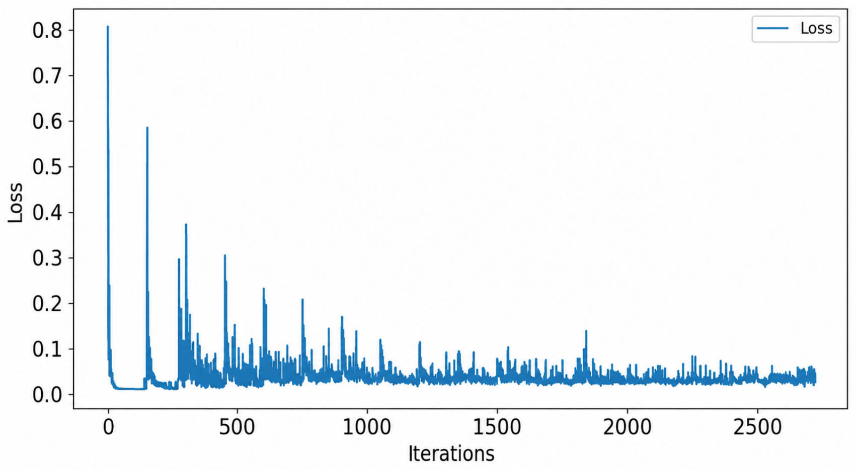
The bus departure process was discretized into a sequential decision-making process with a time step of 1 min, and the DQN algorithm was used to optimize the departure intervals. In the implementation, the DQN used an online Q-network and a target Q-network with the same architecture. The neural network contained two fully connected hidden layers with 512 neurons in each layer and ReLU activation, followed by a linear output layer for Q-values. The main training parameters were set as follows: learning rate 0.001, discount factor 0.90, replay-buffer capacity 5000, mini-batch size 64, target-network update frequency of 150 learning steps, and 500 training episodes. The variation in loss values after model training is shown in Figure 15. As the number of training iterations increases, the loss value gradually stabilizes after approximately 2000 iterations, indicating that the DQN model has learned a stable departure strategy.
Figure 15.
Iterative change in loss value.
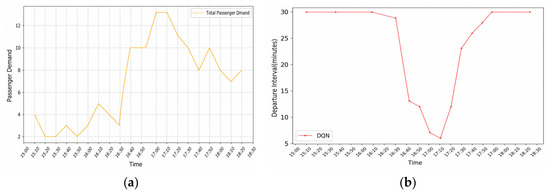
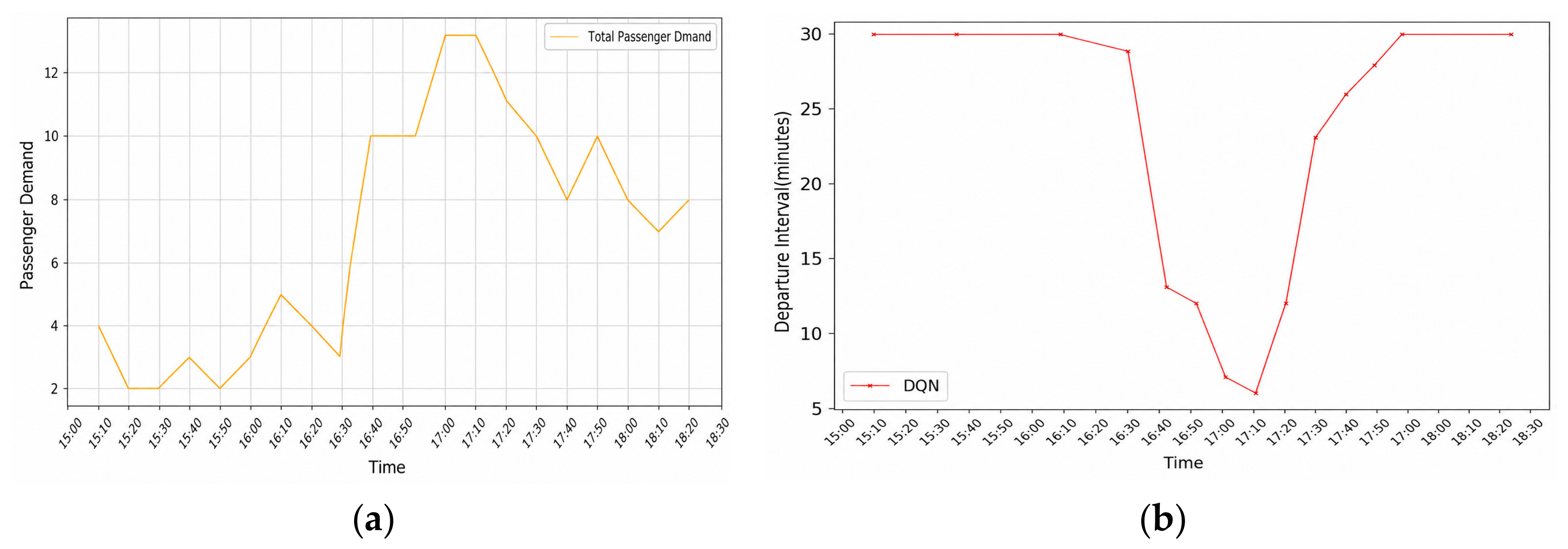
After model convergence, a customized bus departure timetable was generated, and the relationship between passenger demand variation and departure intervals was analyzed. The variation in passenger demand during the service period and the trend of customized bus departure intervals are shown in Figure 16. By comparing the two figures, passenger demand was low during 15:00–16:00, and the model generated longer departure intervals. In contrast, passenger demand peaked during 16:50–17:30, and the model correspondingly shortened departure intervals and increased departure frequency. These results indicate that the DQN method can dynamically adjust the departure strategy according to changes in passenger demand intensity, thereby reducing waiting time while avoiding ineffective departures during low-demand periods.
Figure 16.
(a) Passenger demand trend during the service period; (b) departure interval of customized buses during the service period.
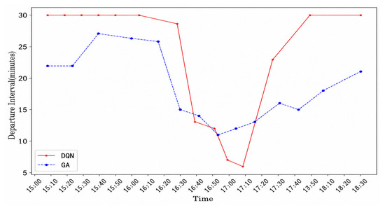
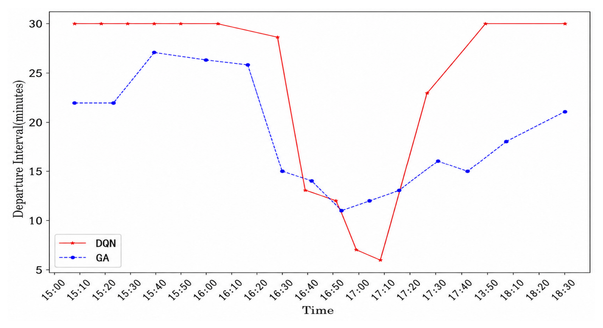
To further verify the effectiveness of the DQN method in timetable optimization, this paper selected the Genetic Algorithm (GA) as a benchmark method to optimize the departure intervals under the same demand conditions and parameter settings. The departure-interval trends obtained by the two methods are shown in Figure 17.
Figure 17.
Comparison of departure intervals based on DQN and GA.
On this basis, the number of departures generated by GA and DQN in different time periods was further summarized to compare the responsiveness of the two methods to peak and off-peak demand variations, as shown in Table 7. The results show that, compared with GA, the DQN can adjust departure intervals more flexibly according to demand changes. During the peak demand period from 16:30 to 17:30, DQN produces shorter departure intervals and higher departure frequency. During off-peak periods, DQN extends departure interval, thereby reducing unnecessary operational costs. This indicates that the DQN has superior adaptive capability between peak and off-peak periods.
Table 7.
Departure frequency statistics for each time period obtained by different methods.
Further analysis of the key operating indicators of the two methods is shown in Table 8. Compared with GA, the DQN reduces the total number of departures from 13 to 11, increases the average passenger load factor from 62.7% to 74.1%, and reduces the average waiting time from 4.1 min to 3.2 min. These results demonstrate that the DQN reduces the number of departures without sacrificing service quality. Instead, it achieves better performance in terms of both passenger waiting experience and vehicle utilization.
Table 8.
Comparison indicators of different methods.
6.5. Social Benefits
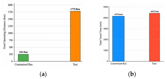
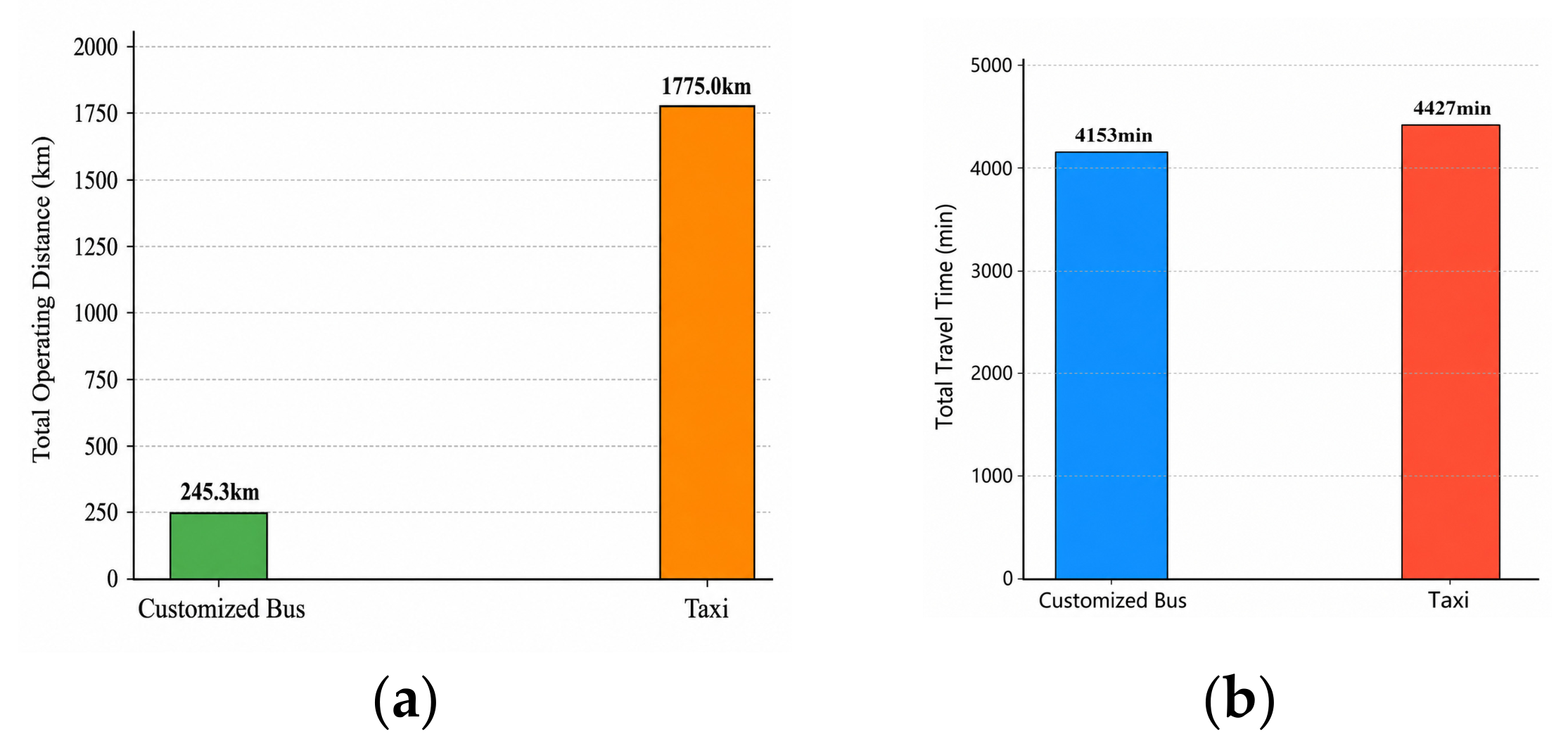
Finally, this paper analyzes the potential social benefits of customized bus services from the perspective of travel-mode substitution. Both customized buses and taxis can satisfy relatively direct travel needs, but customized buses have significant advantages in intensive transportation and green mobility. Taking Route 2 as an example, this paper uses the travel data of the 163 passengers served by this route to compare customized bus and taxis in terms of total operating distance and travel time, as shown in Figure 18.
Figure 18.
(a) Comparison of total travel distance between customized bus and taxi modes; (b) comparison of total travel time between customized bus and taxi modes.
In terms of total operating distance, if all passenger demands were served by taxis based on their OD coordinates, the total distance would be approximately 1775 km. In contrast, the customized bus mode requires only 245.3 km based on the route length and departure frequency of Route 2, representing an 86% reduction compared to taxis. This is mainly because customized buses can integrate multiple passenger demands through stop aggregation and route planning, thereby providing concentrated commuting services with lower vehicle mileage. These findings demonstrate that customized buses can provide higher transport capacity than taxis and effectively reduce road resource occupation and potential vehicle empty mileage.
Regarding total travel time, based on the departure and arrival times in the passenger travel data, the total travel time in the taxi mode is about 4427 min. In contrast, the customized bus mode requires only 4153 min, calculated based on passengers’ boarding and alighting stops and inter-stop travel times. This indicates that customized bus services can save each passenger an average of 1.7 min. These findings demonstrate that the proposed route and timetable scheme can not only reduce the total vehicle operating distance, but also minimize passengers waiting time through optimized departure scheduling, thereby improving overall travel efficiency.
In summary, while meeting specific commuting needs, customized bus services show lower total operating distance and shorter total travel time than taxis in the case of Route 2. This indicates that customized buses have positive for alleviating peak-hour traffic congestion, improving road resource utilization, and promoting green and low-carbon travel. Therefore, the reasonable planning and organization of customized bus services in urban commuting corridors can not only improve passengers’ travel experience but also generate broader traffic and social benefits.
7. Conclusions
This paper proposes an integrated customized bus planning framework based on taxi GPS data for urban peak-hour commuting scenarios. The framework covers the complete process from potential demand identification to stop selection, route planning, and departure timetable optimization. Stable commuting demand is first identified from taxi trajectory data, and candidate stops are then selected using the proposed IDK-SG algorithm. Route planning and dynamic departure intervals are further optimized using a genetic algorithm and deep reinforcement learning, respectively.
The case study using Chongqing taxi GPS data verifies the effectiveness of the proposed framework in transforming trajectory-derived commuting demand into customized bus planning decisions. The identified stable commuting zone pairs were refined into boarding and alighting stops, and the optimized routes covered the main demand areas while satisfying practical constraints on route length and stop number. The timetable optimization results further show that adaptive departure scheduling can better match time-varying passenger demand and improve the balance between service quality and vehicle utilization. These findings indicate that the main novelty of this study lies in establishing a problem-oriented and sequentially coupled planning framework that links trajectory-based demand screening, noise-robust stop extraction, a bi-objective optimization model for route planning, and DQN-based departure scheduling.
This study also has limitations. First, although the framework is described as integrated, the current implementation links demand identification, stop and route planning, and timetable optimization in a sequential manner, while fully joint optimization among these modules has not yet been achieved. Second, the empirical validation is based on one city, and additional case studies are needed to test generalizability under different urban forms, passenger habits, and traffic conditions. Third, the sensitivity of the results to key parameters, including clustering thresholds, objective-function weights, vehicle capacity, and departure-interval bounds, should be examined more systematically. Future research will incorporate multi-source traffic data, dynamic road-network states, multiple vehicle types and capacities, autonomous or semi-autonomous customized bus services, and multi-route coordinated optimization to improve the adaptability and application potential of the proposed framework.
Author Contributions
Conceptualization, Y.D. and J.X.; methodology, Y.D.; software, J.X.; validation, Y.D., J.X. and D.X.; formal analysis, Y.D.; investigation, J.X.; resources, D.X.; data curation, J.X.; writing—original draft preparation, Y.D.; writing—review and editing, D.X.; visualization, J.X.; supervision, D.X.; project administration, D.X.; funding acquisition, D.X. All authors have read and agreed to the published version of the manuscript.
Funding
This research was supported by the Chongqing Postdoctoral Science Foundation (CSTB2023NSCQ-BHX0220), the National Natural Science Foundation of China (NSFC) Youth Project (NO. 62402072), and the Chongqing Municipal Education Commission Science and Technology Research Project (KJQN202300709).
Data Availability Statement
The data presented in this study are available on request from the corresponding author as the data were obtained from an anonymized taxi operation data dataset for research purposes. Because the raw GPS trajectories contain sensitive vehicle and trip information and are subject to data-use restrictions, they are not publicly deposited in an online repository.
Conflicts of Interest
The authors declare no conflict of interest.
References
- Cervero, R. Paratransit in America: Redefining Mass Transportation; Praeger Publishers: Westport, CT, USA, 1997. [Google Scholar]
- Vansteenwegen, P.; Melis, L.; Aktaş, D.; Montenegro, B.D.G.; Vieira, F.S.; Sörensen, K. A survey on demand-responsive public bus systems. Transp. Res. Part C Emerg. Technol. 2022, 137, 103573. [Google Scholar] [CrossRef] [Scilit]
- Liu, T.; Ceder, A.A. Analysis of a new public-transport-service concept: Customized bus in China. Transp. Policy 2015, 39, 63–76. [Google Scholar] [CrossRef] [Scilit]
- Wang, Y.; Hu, Z.; Huang, H.; Lu, Z.; Wen, X. Optimization for Customized Bus Stop Planning, Order Schedule, and Routing Design in On-Demand Urban Mobility. IEEE Internet Things J. 2023, 11, 10239–10251. [Google Scholar] [CrossRef] [Scilit]
- Toole, J.L.; Colak, S.; Sturt, B.; Alexander, L.P.; Evsukoff, A.; González, M.C. The path most traveled: Travel demand estimation using big data resources. Transp. Res. Part C Emerg. Technol. 2015, 58, 162–177. [Google Scholar] [CrossRef] [Scilit]
- Yu, H.; Guo, X.; Luo, X.; Bian, W.; Zhang, T. Construct trip graphs by using taxi trajectory data. Data Sci. Eng. 2023, 8, 1–22. [Google Scholar] [CrossRef] [Scilit]
- Wang, K.; Chen, W. Customized bus route planning based on taxi order data in a’many-to-one’scenario. In International Conference on Smart Transportation and City Engineering (STCE 2023); SPIE: Bellingham, DC, USA, 2024; Volume 13018, pp. 490–500. [Google Scholar]
- Xia, D.; Zheng, L.; Cai, X.; Liu, W.; Sun, D. Urban customized bus design for private car commuters. IEEE Internet Things J. 2022, 9, 21723–21735. [Google Scholar] [CrossRef] [Scilit]
- Melo, S.; Gomes, R.; Abbasi, R.; Arantes, A. Demand-responsive transport for urban mobility: Integrating mobile data analytics to enhance public transportation systems. Sustainability 2024, 16, 4367. [Google Scholar] [CrossRef] [Scilit]
- Li, W.; Zheng, L.; Wu, X.; Tang, X.; Xiao, S.; Zhao, M.; Sun, D. Exploring Potential Customized Bus Passengers Across Private Car Trajectory Data. IEEE Trans. Intell. Transp. Syst. 2024, 25, 21278–21296. [Google Scholar] [CrossRef] [Scilit]
- Lyu, Y.; Chow, C.Y.; Lee, V.C.S.; Li, Y.; Zeng, J. T2CBS: Mining taxi trajectories for customized bus systems. In 2016 IEEE Conference on Computer Communications Workshops (INFOCOM WKSHPS); IEEE: New York, NY, USA, 2016; pp. 441–446. [Google Scholar]
- Ester, M.; Kriegel, H.P.; Sander, J.; Xu, X. A density-based algorithm for discovering clusters in large spatial databases with noise. Kdd 1996, 96, 226–231. [Google Scholar]
- Lloyd, S. Least squares quantization in PCM. IEEE Trans. Inf. Theory 1982, 28, 129–137. [Google Scholar] [CrossRef] [Scilit]
- Rousseeuw, P.J. Silhouettes: A graphical aid to the interpretation and validation of cluster analysis. J. Comput. Appl. Math. 1987, 20, 53–65. [Google Scholar] [CrossRef] [Scilit]
- Yuan, T.; Liu, H.; Wang, Y.; Yang, F.; Gu, Q.; Wang, Y. Customized Bus Stop Location Model Based on Dual Population Adaptive Immune Algorithm. Mathematics 2024, 12, 2382. [Google Scholar] [CrossRef] [Scilit]
- Tian, Y.; Yang, D.; Wang, J.; Lin, W.; Jiang, Y.; An, S. Designing and planning sustainable customized bus service for departing attendees of planned special events: A two-phase methodology integrating data-driven and demand-responsive. Sustain. Cities Soc. 2023, 96, 104630. [Google Scholar] [CrossRef] [Scilit]
- Ma, D.; Fang, B.; Ma, W.; Wu, X.; Jin, S. Potential routes extraction for urban customized bus based on vehicle trajectory clustering. IEEE Trans. Intell. Transp. Syst. 2023, 24, 11878–11888. [Google Scholar] [CrossRef] [Scilit]
- Toth, P.; Vigo, D. Vehicle Routing: Problems, Methods, and Applications; Society for Industrial and Applied Mathematics: Philadelphia, PA, USA, 2014. [Google Scholar]
- Schöbel, A.; Zhou-Kangas, Y. The price of multiobjective robustness: Analyzing solution sets to uncertain multiobjective problems. Eur. J. Oper. Res. 2021, 291, 782–793. [Google Scholar] [CrossRef] [Scilit]
- Zhen, L.; He, X.; Wang, S.; Wu, J.; Liu, K. Vehicle routing for customized on-demand bus services. IISE Trans. 2023, 55, 1277–1294. [Google Scholar] [CrossRef] [Scilit]
- Asghari, M.; Al-e, S.M.J.M.; Rekik, Y. Environmental and social implications of incorporating carpooling service on a customized bus system. Comput. Oper. Res. 2022, 142, 105724. [Google Scholar] [CrossRef] [Scilit]
- Chen, F.; Lu, Y.; Liu, L.; Zhu, Q. Route Optimization of Customized Buses Based on Optimistic and Pessimistic Values. IEEE Access 2023, 11, 11016–11023. [Google Scholar] [CrossRef] [Scilit]
- Gkiotsalitis, K.; Alesiani, F. Robust timetable optimization for bus lines subject to resource and regulatory constraints. Transp. Res. Part E Logist. Transp. Rev. 2019, 128, 30–51. [Google Scholar] [CrossRef] [Scilit]
- Xia, D.; Ma, J.; Azadeh, S.S.; Zhang, W. Data-driven distributionally robust timetabling and dynamic-capacity allocation for automated bus systems with modular vehicles. Transp. Res. Part C Emerg. Technol. 2023, 155, 104314. [Google Scholar] [CrossRef] [Scilit]
- Liu, Y.; Luo, X.; Wei, X.; Yu, Y.; Tang, J. Robust optimization model for single line dynamic bus dispatching. Sustainability 2021, 14, 73. [Google Scholar] [CrossRef] [Scilit]
- Dou, X.; Li, T. Multi-objective bus timetable coordination considering travel time uncertainty. Processes 2023, 11, 574. [Google Scholar] [CrossRef] [Scilit]
- Liu, T.; Ji, W.; Gkiotsalitis, K.; Cats, O. Optimizing public transport transfers by integrating timetable coordination and vehicle scheduling. Comput. Ind. Eng. 2023, 184, 109577. [Google Scholar] [CrossRef] [Scilit]
- Yan, H.; Cui, Z.; Chen, X.; Ma, X. Distributed multiagent deep reinforcement learning for multiline dynamic bus timetable optimization. IEEE Trans. Ind. Inform. 2022, 19, 469–479. [Google Scholar] [CrossRef] [Scilit]
- Ai, G.; Zuo, X.; Chen, G.; Wu, B. Deep reinforcement learning based dynamic optimization of bus timetable. Appl. Soft Comput. 2022, 131, 109752. [Google Scholar] [CrossRef] [Scilit]
- Wang, J.; Sun, L. Robust dynamic bus control: A distributional multi-agent reinforcement learning approach. IEEE Trans. Intell. Transp. Syst. 2022, 24, 4075–4088. [Google Scholar] [CrossRef] [Scilit]
- Song, M.; Stević, Ž.; Badi, I.; Marinković, D.; Lv, Y.; Zhong, K. Assessing public acceptance of autonomous vehicles using a novel IRN PIPRECIA-IRN AROMAN model. Facta Univ. Ser. Mech. Eng. 2025, 23, 127–145. [Google Scholar] [CrossRef] [Scilit]
- Holland, J.H. Adaptation in Natural and Artificial Systems; University of Michigan Press: Ann Arbor, MI, USA, 1975. [Google Scholar]
- Sastry, K.; Goldberg, D.E.; Kendall, G. Genetic algorithms. In Search Methodologies: Introductory Tutorials in Optimization and Decision Support Techniques; Springer: Boston, MA, USA, 2013; pp. 93–117. [Google Scholar]
- Puterman, M.L. Markov decision processes. Handb. Oper. Res. Manag. Sci. 1990, 2, 331–434. [Google Scholar] [CrossRef] [Scilit]
- Sutton, R.S.; Barto, A.G. Reinforcement Learning: An Introduction, 2nd ed.; The MIT Press: Cambridge, MA, USA, 2018. [Google Scholar]
- Mnih, V.; Kavukcuoglu, K.; Silver, D.; Rusu, A.A.; Veness, J.; Bellemare, M.G.; Graves, A.; Riedmiller, M.; Fidjeland, A.K.; Ostrovski, G.; et al. Human-level control through deep reinforcement learning. Nature 2015, 518, 529–533. [Google Scholar] [CrossRef] [Scilit] [PubMed]

Disclaimer/Publisher’s Note: The statements, opinions and data contained in all publications are solely those of the individual author(s) and contributor(s) and not of MDPI and/or the editor(s). MDPI and/or the editor(s) disclaim responsibility for any injury to people or property resulting from any ideas, methods, instructions or products referred to in the content. |
© 2026 by the authors. Licensee MDPI, Basel, Switzerland. This article is an open access article distributed under the terms and conditions of the Creative Commons Attribution (CC BY) license.