Adaptive SVG-Based Supplementary Damping Control for Wideband Oscillation Mitigation in PV-Integrated Distribution Network

Abstract

When photovoltaic (PV) power plants are connected to weak alternating current (AC) grids, the interaction between the plant and grid may induce wideband oscillation, posing a serious threat to the stability of grid-connected PV systems. To address this problem, this paper proposes an oscillation suppression method based on adaptive supplementary damping control of a Static Var Generator (SVG). First, a sequence impedance model of a PV power plant integrated with an SVG is established, and the Nyquist criterion is employed to analyze the mechanism underlying wideband oscillations. Then, a supplementary damping controller implemented in the SVG is designed to reshape the impedance characteristics of the PV power plant and enhance system damping. Furthermore, a Variational Mode Decomposition–Prony modal identification algorithm is introduced to extract oscillation mode information in real time. Based on the identified oscillation frequency, the parameters of the damping controller are adaptively adjusted, thereby improving the suppression capability for wideband oscillations with varying frequencies. Finally, a grid-connected PV power plant model with an SVG is developed, and the performance of the proposed adaptive suppression strategy is compared with that of conventional supplementary damping control. The results demonstrate that the proposed strategy provides stronger robustness and adaptability, effectively suppresses wideband oscillations under different operating conditions, and improves the stability of grid-connected PV systems.

1. Introduction

Renewable energy technologies have received increasing attention because of global energy shortages and the transition toward low-carbon power systems. Among these technologies, photovoltaic (PV) generation has become one of the most widely deployed renewable energy sources due to its cleanliness, abundance, and broad geographical availability. However, as the penetration level of PV generation in distribution networks continues to increase, the dynamic interaction between PV converter control loops and weak-grid impedance may induce wideband oscillations. These oscillations, especially sub-/super-synchronous oscillations, can deteriorate power quality and pose a significant threat to the stability and secure operation of PV-integrated distribution networks.

Impedance-based stability analysis has been widely used to investigate the oscillation mechanisms of converter-dominated power systems. The sequence-impedance modeling method provides an effective framework for characterizing the frequency-domain interaction between grid-connected converters and weak AC grids [1]. Based on this framework, various mitigation strategies have been developed to suppress wideband oscillations. Existing methods can generally be classified into two categories: intrinsic converter control enhancement and supplementary damping injection, which can be implemented either on the converter side or on the grid side.

Intrinsic converter control enhancement aims to improve system stability by reshaping the small-signal impedance of converters and/or reducing frequency coupling through controller design. This category mainly includes controller-parameter retuning and control-structure modification. For example, ref. [2] tunes PV converter control parameters according to grid impedance characteristics to improve weak-grid stability, while ref. [3] analyzes the influence of different control loops on converter impedance and optimizes controller parameters to increase the stability margin. However, parameter retuning may compromise other aspects of converter performance, such as dynamic response and power quality, under varying operating conditions. In terms of control-structure modification, ref. [4] adopts a symmetrical phase-locked loop (PLL) to mitigate frequency coupling caused by dq-frame asymmetry, whereas refs. [5,6] replace the conventional inner-loop proportional–integral (PI) controller with nonlinear or robust controllers, such as sliding-mode and H∞ controllers, to enhance system robustness. Nevertheless, these methods usually involve higher design complexity and more difficult parameter tuning, which may limit their engineering applicability in large-scale PV plants.

Supplementary damping injection suppresses oscillations by introducing an additional damping channel that injects compensating sub-/super-synchronous current or voltage components. For instance, ref. [7] proposes a dual-channel supplementary damping controller and verifies its effectiveness through impedance-based analysis. In addition, refs. [8,9] implement supplementary damping controllers on grid-side compensation devices, such as static var generators (SVGs), static synchronous compensators, and other flexible AC transmission devices, to provide additional damping for weak-grid systems. Compared with converter-side control modification, grid-side supplementary damping can avoid modifying the control structure of each distributed PV inverter and is therefore more suitable for practical PV plants with numerous converter units. However, a major limitation of conventional supplementary damping control is its sensitivity to oscillation-frequency drift and operating-point variations. Once the dominant oscillation frequency deviates from the preset tuning range, the damping performance may deteriorate significantly.

Recent studies have further extended oscillation mitigation research toward grid-forming converters, virtual synchronous machine control, adaptive impedance control, and data-driven or signal-processing-assisted oscillation detection. For example, ref. [10] enhances damping in grid-forming permanent-magnet synchronous generator systems by introducing the DC-link voltage error into the reactive-power loop. Ref. [11] investigates adaptive virtual-impedance droop control for parallel inverters, demonstrating the potential of adaptive impedance shaping for improving converter stability. Related work has investigated oscillation suppression, impedance reshaping, frequency-coupling/modal analysis, and damping control in renewable-energy-dominated systems, including wind farms, DFIG-based systems, offshore MVDC systems, and high-renewable-penetration grids [12,13,14,15,16,17,18]. Similar virtual-damping concepts have also been extended to other power-electronic drive systems [19]. In addition, impedance-based sensitivity analysis has been applied to identify key parameters affecting dynamic stability in converter-dominated systems [20]. Recent studies on PV grid integration have also emphasized advanced modeling, control strategies, and simulation-based validation for improving the performance of grid-connected PV systems [21]. For PV-specific oscillation suppression, model-free adaptive control and grid-forming PV damping enhancement strategies have been investigated in recent works [22,23]. Furthermore, comparative studies of grid-following and grid-forming inverter impedance characteristics have provided useful insights into the stability differences between different converter control paradigms [24], while comprehensive reviews have summarized the mechanisms and mitigation methods of wideband oscillations in PV-dominated weak grids [25].

Although these studies have advanced the understanding and mitigation of converter-driven oscillations, several practical challenges remain. First, many converter-side control methods require modification of individual inverter controllers, which is difficult and costly for existing PV plants consisting of multiple distributed inverter units. Second, fixed-parameter damping controllers are usually designed for a specific oscillation frequency or operating condition, and their effectiveness may decline when grid strength, converter parameters, or oscillation modes change. Third, wideband oscillations in weak-grid PV systems may occur over a broad frequency range, making it necessary for the damping controller to track the dominant oscillation mode and update its parameters online. Therefore, a practical grid-side damping strategy that uses existing SVG equipment and provides adaptive frequency-tracking capability is required.

To address these issues, this paper proposes an SVG-based adaptive supplementary damping control method for suppressing wideband oscillations in grid-connected PV systems. First, a sequence-impedance model of an SVG-integrated PV plant is established, and the oscillation mechanism is analyzed using the Nyquist stability criterion. On this basis, an SVG supplementary damping controller is designed to reshape the system impedance and enhance damping in critical sub-/super-synchronous frequency bands. Then, a variational mode decomposition–Prony (VMD–Prony) modal identification method is employed to extract the dominant oscillation frequency from measured signals. According to the identified oscillation mode, the center frequency of the damping controller is adaptively updated, enabling the proposed controller to maintain effective oscillation suppression under varying grid strengths and operating conditions. The effectiveness of the proposed method is verified using a weak-grid PV plant model developed in MATLAB 2024a under multiple operating scenarios.

The main contributions of this paper are summarized as follows:

(1) A sequence-impedance-based analysis framework is established for an SVG-integrated PV plant, and the mechanism of wideband oscillation caused by the interaction between PV converter controls and weak-grid impedance is clarified using the Nyquist stability criterion.

(2) An SVG-based supplementary damping controller is designed from an impedance-reshaping perspective to improve the damping characteristics of PV-integrated weak-grid systems in critical sub-/super-synchronous frequency bands.

(3) A VMD–Prony-based adaptive tuning strategy is proposed to identify the dominant oscillation frequency online and update the center frequency of the SVG damping controller, thereby improving the robustness of oscillation suppression under varying operating conditions.

The remainder of this paper is organized as follows. Section 2 presents the sequence-impedance modeling of an SVG-integrated PV power plant and analyzes the mechanism of wideband oscillations. Section 3 introduces the proposed SVG-based adaptive supplementary damping control method, including the VMD–Prony-based modal identification method and the adaptive damping control strategy. Section 4 presents case studies and simulations to verify the accuracy of the impedance model and the effectiveness of the proposed oscillation-suppression method. Section 5 concludes the paper and summarizes the main findings.

2. Oscillation Mechanism of the SVG-Integrated PV Plant

2.1. Sequence Impedance Model

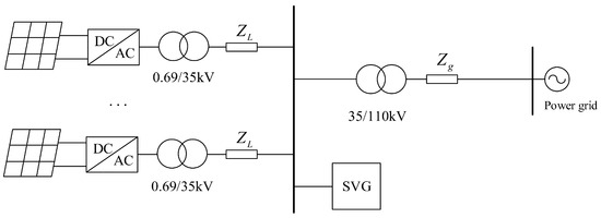
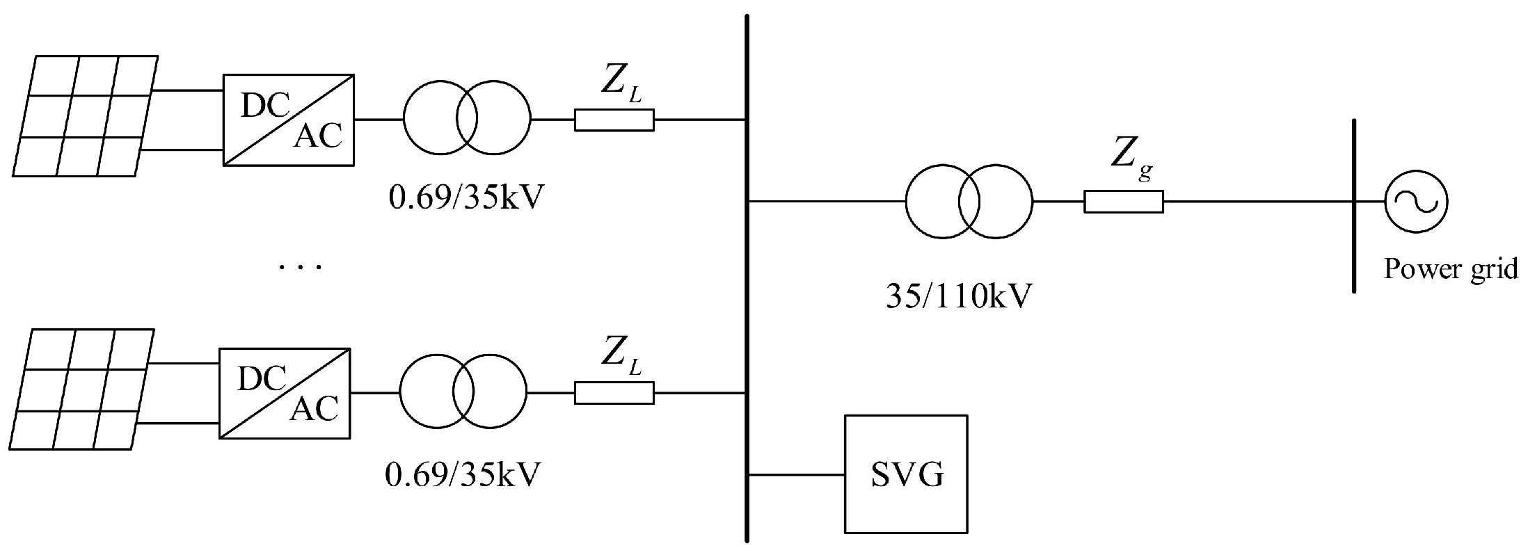
Figure 1 shows a simplified single-line diagram of the studied SVG-integrated PV plant connected to a weak grid. For clarity, only representative PV branches are shown, and the ellipsis denotes the remaining PV converter units and collector-network connections. Each representative PV branch is connected to the 35 kV collector bus through a 0.69 kV/35 kV step-up transformer and a collection cable. The SVG is connected to the 35 kV collector bus, and the entire PV plant is connected to the external 110 kV grid through a 35 kV/110 kV step-up transformer. In Figure 1, Z_L represents the impedance of the PV collection cable, and Z_g represents the equivalent impedance of the 110 kV external grid.

Figure 1. Simplified single-line diagram of the SVG-integrated PV plant connected to a weak grid.

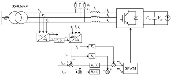
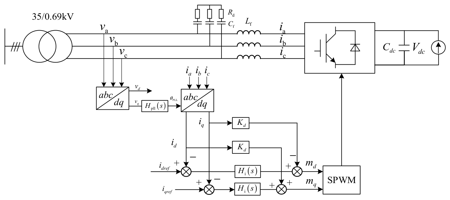
The main circuit and control structure of a typical photovoltaic converter are shown in Figure 2. In the figure, C_dc is the DC capacitor, V_dc is the DC-link voltage, v_a, v_b, and v_c are the converter output voltages, i_a, i_b, and i_c are the converter output currents, L_f is the filter inductor, i_dref and i_qref are the reference values of the d- and q- axis currents in the inner current-control loop. H_i(s) and H_pll(s) are the transfer functions of the inner current controller and the phase-locked loop (PLL), respectively, as given in Appendix A Equation (A1). In addition, θ_pll is the phase angle deviation generated by the PLL, and K_d is the cross-decoupling coefficient.

Figure 2. Main circuit and control structure of a typical grid-connected PV converter.

Based on the harmonic linearization method, the phase-A output voltage of the inner current-control loop under positive- and negative-sequence perturbations can be expressed as follows:

$$\begin{array}{l}{m}_{\mathrm{ap}}[f]=\mp \mathrm{j}{\displaystyle \frac{1}{2}}{G}_{\mathrm{pll}}(s\mp \mathrm{j}2\pi f_1)H_i(s\mp \mathrm{j}2\pi f_1)(-I_{\mathrm{qref}}\pm \mathrm{j}{I}_{\mathrm{dref}}){\mathbf{V}}_{\mathrm{p}}+\\ \left[-H_i(s\mp \mathrm{j}2\pi f_1)\pm \mathrm{j}{K}_{\mathrm{d}}\right]{\mathbf{I}}_{\mathrm{p}} f=\pm f_{\mathrm{p}}\end{array}$$

(1)

$$\begin{array}{l}{m}_{\mathrm{an}}[f]=\pm j{\displaystyle \frac{1}{2}}{G}_{pll}(s\pm j2\pi f_1)H_i(s\pm j2\pi f_1)(-I_{\mathrm{qref}}\mp \mathrm{j}{I}_{\mathrm{dref}}){\mathbf{V}}_{\mathrm{n}}+\\ [-H_i\left(s\pm j2\pi f_1\right)\mp j{K}_{\mathrm{d}}]{\mathbf{I}}_{\mathrm{n}} f=\pm f_{\mathrm{n}}\end{array}$$

(2)

where V_p and V_n are injected positive- and negative-sequence small disturbance voltages, I_p and I_n are positive- and negative-sequence disturbance current responses, whose expressions are shown in Appendix A Equation (A2). G_pll(s) is the closed-loop transfer function of the PLL, as given in Appendix A Equation (A3). f₁, f_p, and f_n are the fundamental frequency, the positive-sequence disturbance frequency, and the negative-sequence disturbance frequency, respectively.

According to the circuit topology of the PV converter shown in Figure 2, the voltage- current relationship at the point of common coupling (PCC) can be written as

$$s{L}_f{i}_a={\displaystyle \frac{1}{2}}{V}_{dc}{m}_a-v_a$$

(3)

By substituting Equations (1) and (2) into Equation (3), the positive- and negative-sequence impedance models of the PV converter can be derived as:

$$Z_{\mathrm{P}\mathrm{V},\mathrm{p}}\left(s\right)=-{\displaystyle \frac{{\mathbf{V}}_{\mathrm{p}}}{{\mathbf{I}}_{\mathrm{p}}}}={\displaystyle \frac{s{L}_{\mathrm{f}}+\frac{V_{\mathrm{d}\mathrm{c}}}{2}\left[H_{\mathrm{i}}(s-\mathrm{j}2\pi f_1)-\mathrm{j}{K}_{\mathrm{d}}\right]}{1-\frac{V_{\mathrm{d}\mathrm{c}}}{4}{G}_{\mathrm{pll}}(s-j2\pi f_1)H_{\mathrm{i}}(s-\mathrm{j}2\pi f_1)(I_{\mathrm{dref}}+\mathrm{j}{I}_{\mathrm{qref}})}}$$

(4)

$$Z_{\mathrm{P}\mathrm{V},\mathrm{n}}\left(s\right)=-{\displaystyle \frac{{\mathbf{V}}_{\mathrm{n}}}{{\mathbf{I}}_{\mathrm{n}}}}={\displaystyle \frac{s{L}_{\mathrm{f}}+\frac{V_{\mathrm{dc}}}{2}\left[H_{\mathrm{i}}(s+\mathrm{j}2\pi f_1)+\mathrm{j}{K}_{\mathrm{d}}\right]}{1-\frac{V_{\mathrm{dc}}}{4}{G}_{\mathrm{pll}}\left(s+\mathrm{j}2\pi f_1\right)H_{\mathrm{i}}(s+\mathrm{j}2\pi f_1)(I_{\mathrm{dref}}-\mathrm{j}{I}_{\mathrm{qref}})}}$$

(5)

The sequence-impedance modeling procedure for the SVG is similar to that for the PV converter. The derived positive- and negative-sequence impedances of the SVG are given in Appendix A Equations (A4) and (A5), respectively.

After deriving the sequence impedances of the individual PV converter and the SVG, the plant-level aggregated impedance must be obtained to characterize the frequency-domain interaction between the PV plant and the external grid. In practical PV power plants, multiple converter units are interconnected through collection cables, transformers, and busbars. Therefore, the impedance of a single converter cannot fully represent the overall impedance characteristics of the entire plant.

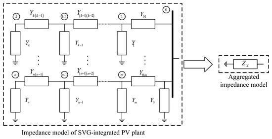
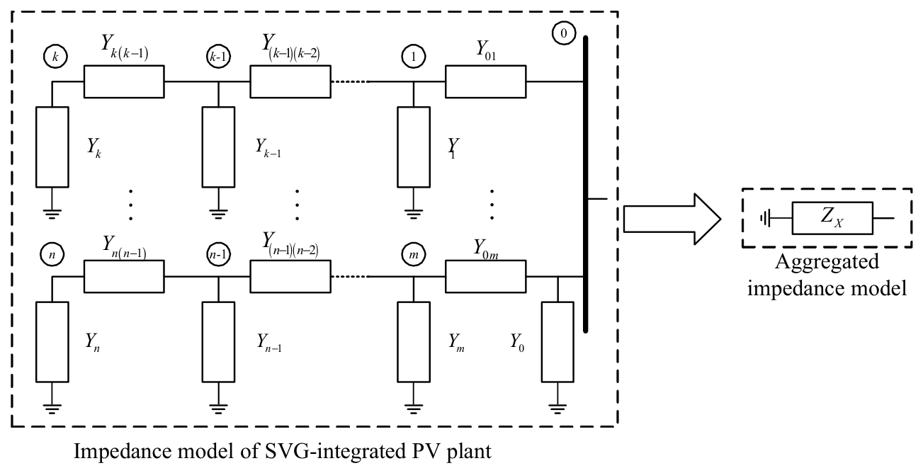
Although Figure 1 presents a simplified single-line diagram, the actual collector system of a PV plant may contain multiple converter terminals, transformer terminals, collection-cable sections, and busbar nodes. For aggregated impedance calculation, these components can be represented by the generalized nodal-admittance network shown in Figure 3. In this network, node 0 denotes the PCC at the 35 kV collector bus. Y_k(s) represents the shunt admittance connected to node k, Y_kn(s) denotes the connection admittance between nodes k and n, and Z_x(s) is the aggregated equivalent impedance of the SVG-integrated PV plant viewed from the PCC. The external grid impedance Z_g(s) is treated separately in the stability analysis and is not included in the calculation of Z_x(s).

Figure 3. Generalized nodal-admittance network for calculating the aggregated impedance Z_x(s) of the SVG-integrated PV plant.

To calculate the driving-point impedance viewed from the PCC, all independent sources inside the PV plant are suppressed, while the PV converters and the SVG are represented by their small-signal positive-sequence admittances. Let V₀ and I₀ be the test voltage and test current at node 0, respectively, and let V_N = [V₁, V₂, …, V_n]^T be the internal node-voltage vector. The partitioned nodal-admittance equation can be written as

$$\left[\begin{array}{l}{I}_0\\ 0\end{array}\right]=\left[\begin{array}{cc}{Y}_0(s)+{\displaystyle \sum _{i=1}^n{Y}_{0i}(s)}& -y_0^T(s)\\ -y_0(s)& Y_N(s)\end{array}\right]\left[\begin{array}{l}{V}_0\\ V_N\end{array}\right]$$

(6)

where Y_N(s) is the internal positive-sequence nodal-admittance matrix after removing node 0, and

$$y_0(s)={[Y_{01}(s),Y_{02}(s),\dots ,Y_{0n}(s)]}^T$$

(7)

is the connection-admittance vector between node 0 and the internal nodes of the PV plant.

By eliminating the internal node voltages V_N, the positive-sequence driving-point admittance viewed from the PCC can be obtained as

$$Y_X(s)=Y_0(s)+{\displaystyle \sum _{i=1}^n{Y}_{0,i}(s)-y_0^T(s)Y_N^{-1}(s)y_0(s)}$$

(8)

Therefore, the aggregated positive-sequence impedance of the SVG-integrated PV plant is expressed as

$$Z_X(s)={\displaystyle \frac{1}{Y_0(s)+{\displaystyle \sum _{i=1}^n{Y}_{0,i}(s)-y_0^T(s)Y_N^{-1}(s)y_0(s)}}}$$

(9)

where Y₀(s) is the shunt admittance connected to node 0. Since the SVG is connected to the 35 kV collector bus, its positive-sequence admittance is included in Y₀(s). All converter, SVG, transformer, and cable impedances are referred to the 35 kV collector-bus side before constructing the nodal-admittance matrix.

2.2. Oscillation Mechanism Analysis

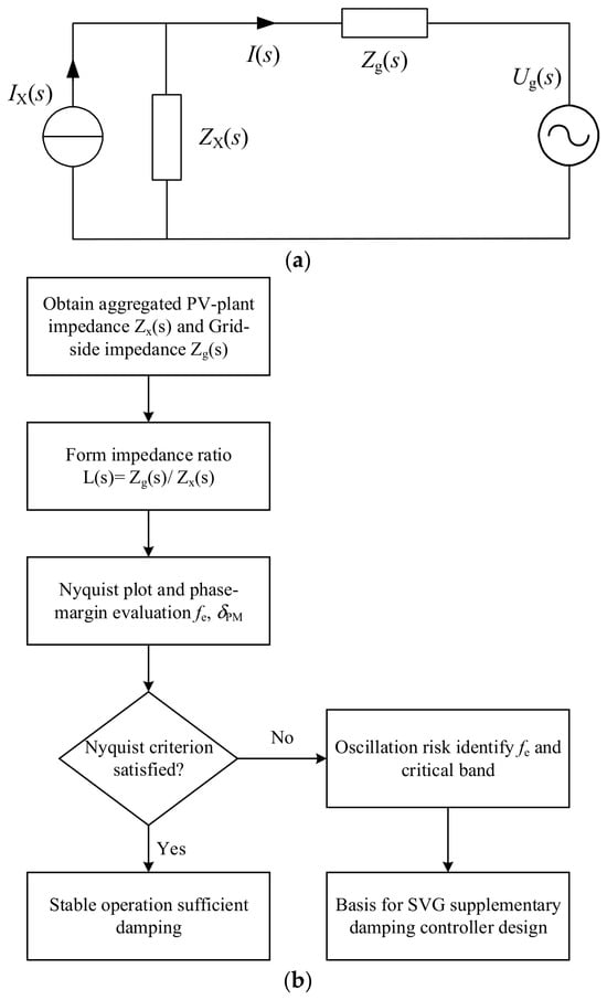
Using the Norton equivalent principle, the SVG-integrated PV plant connected to the external grid can be represented by the equivalent circuit shown in Figure 4. In this model, Z_X(s) is the aggregated impedance of the PV plant, Z_g(s) is the grid-side impedance, U_g(s) is the grid voltage, and I_X(s) represents the equivalent current source of the PV plant.

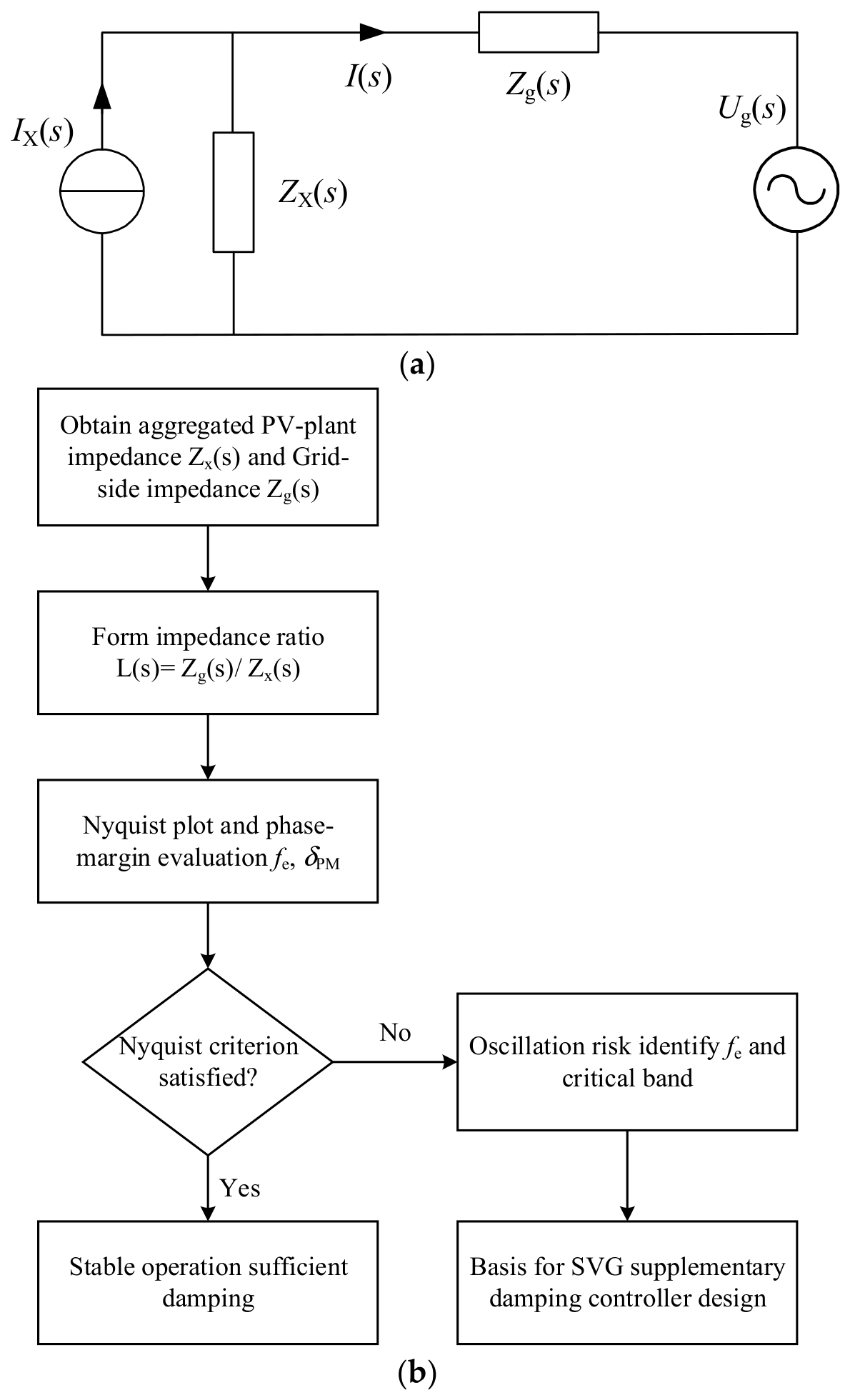
Figure 4. Impedance-based stability analysis of the SVG-integrated PV plant: (a) Norton-equivalent circuit; (b) procedure for impedance-based stability analysis using the Nyquist criterion.

According to the superposition principle, the PCC current in Figure 4 can be expressed as:

$$I(s)={\displaystyle \frac{1}{1+Z_g(s)/Z_X(s)}}\left(I_X(s)-{\displaystyle \frac{U_g(s)}{Z_X(s)}}\right)$$

(10)

In general, the grid voltage U_g(s) is assumed to be stable, and the PV converters and SVG are also stable when connected to an ideal voltage source. Therefore, I_X(s) and U_g (s)/Z_X(s) are stable terms. Under this assumption, the small-signal stability of the PCC current I(s) is mainly determined by the denominator term 1 + Z_g(s)/Z_X(s). In other words, the stability of the SVG-integrated PV plant connected to a weak grid depends on whether the impedance ratio Z_g(s)/Z_X(s) satisfies the Nyquist stability criterion.

At the impedance intersection frequency f_e, where the magnitudes of Z_g(j2πf) and Z_X(j2πf) are equal, the phase margin can be calculated as

$${\delta }_{PM}={180}^{\circ }-\left[\angle Z_g\left(j2\pi f_e\right)-\angle Z_X\left(j2\pi f_e\right)\right]>0$$

(11)

where δ_PM is the system phase margin, and f_e is the frequency at which the |Z_g(j2πf)| and |Z_X(j2πf)| intersect.

The wideband oscillation mechanism can therefore be interpreted from the impedance perspective. When the PV plant exhibits capacitive negative-damping characteristics in the sub-/super-synchronous frequency band, its aggregated impedance Z_X(s) may interact with the inductive impedance of the weak grid Z_g(s). If this interaction occurs near the impedance intersection frequency and the corresponding phase margin becomes negative, the Nyquist stability condition is violated. As a result, small disturbances around the resonant frequency are amplified rather than damped, leading to sub-/super-synchronous oscillations and even system instability.

Therefore, the occurrence of wideband oscillations in an SVG-integrated PV plant is mainly determined by three factors: the negative-damping characteristics introduced by the converter control loops, the inductive impedance characteristics of the weak grid, and the phase margin at the impedance intersection frequency. A weaker grid increases the grid-side impedance and may shift the impedance intersection point into the negative-damping frequency band, thereby increasing the risk of wideband oscillation.

To further clarify the impedance-based stability analysis procedure, Figure 4b summarizes the main steps. First, the sequence-impedance models of the PV converter and SVG are derived. Then, the aggregated impedance Z_X(s) of the PV plant and the grid-side impedance Z_g(s) are obtained. The impedance ratio L(s) = Z_g(s)/Z_X(s) is subsequently evaluated using the Nyquist criterion. If the phase margin at the impedance intersection frequency is negative, the system may exhibit sub-/super-synchronous oscillations. The identified critical frequency and negative-damping band provides the basis for the SVG supplementary damping controller design in Section 3.

3. Adaptive SVG-Based Supplementary Damping Control

In practical PV power plants, a large number of distributed inverters are connected to the collector bus through cables and step-up transformers. If wideband oscillations are suppressed by modifying the control structure of each PV inverter, the implementation process becomes complicated, costly, and difficult to maintain. In contrast, the static var generator (SVG) installed at the point of common coupling (PCC) provides a more practical grid-side damping actuator. By introducing a supplementary damping channel into the SVG control system, the equivalent impedance of the PV plant can be reshaped without modifying the control structure of each PV inverter.

However, the critical oscillation frequency of a PV-integrated weak-grid system is affected by grid strength, converter control parameters, SVG parameters, and operating conditions. A fixed-parameter supplementary damping controller can only provide effective damping within a limited frequency range. Once the dominant oscillation frequency deviates from the preset center frequency, the damping effect may deteriorate. Therefore, an adaptive supplementary damping control strategy is required to track the dominant oscillation mode online and adjust the controller parameters accordingly.

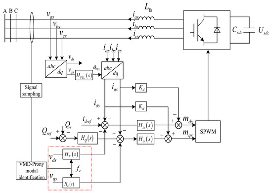
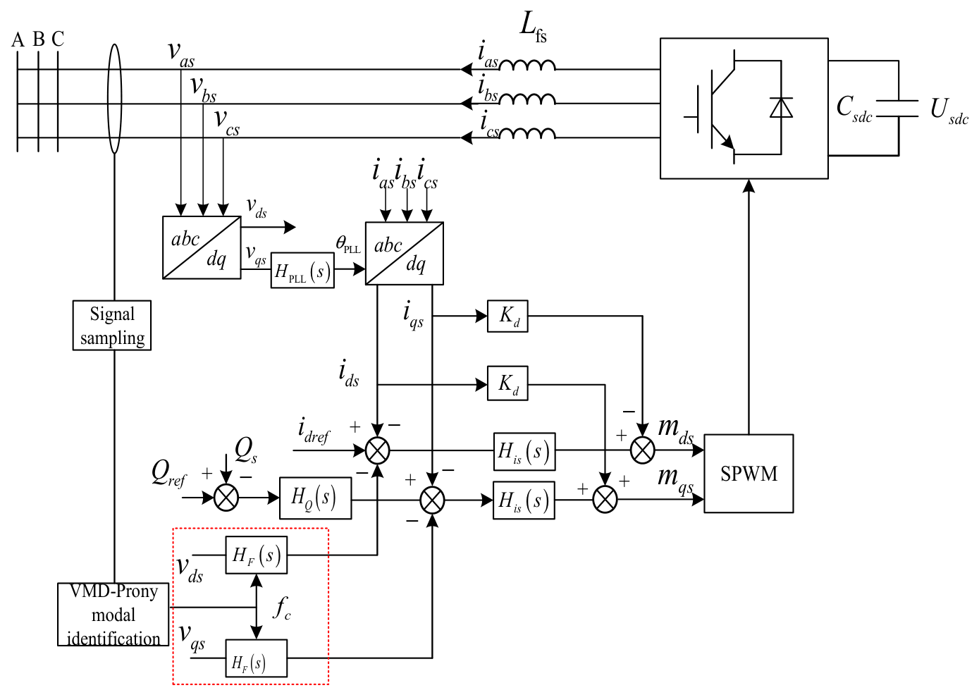
In this paper, a variational mode decomposition–Prony (VMD–Prony) modal identification method is used to extract the dominant oscillation frequency from the measured PCC signal. According to the identified oscillation mode, the center frequency of the SVG supplementary damping controller is updated online. The proposed SVG-based adaptive supplementary damping control structure is shown in Figure 5.

Figure 5. SVG adaptive supplementary damping control structure.

3.1. Principle and Parameter Tuning of SVG Supplementary Damping Control

The SVG supplementary damping controller (SDC) reshapes the impedance characteristics of the SVG by introducing narrow-band voltage-feedback branches into the d- and q-axis control paths. The damping signal is generated from the oscillatory voltage component and superimposed on the SVG modulation signal. In this way, the SVG provides an equivalent positive damping effect in the critical sub-/super-synchronous frequency band, thereby reducing the negative-damping characteristics of the PV plant and improving the stability of the grid-connected system.

The transfer function of the supplementary damping controller, shown by the red dashed block in Figure 5, is expressed as

$$H_F(s)={\displaystyle \frac{2K_R{\omega }_{b}s}{s^2+2{\omega }_{b}s+{\omega }_c^2}}$$

(12)

where ${\omega }_c=2\pi f_c$ is the central angular frequency of the damping controller, f_c is the corresponding center frequency, ${\omega }_b$ is the bandwidth-related cutoff angular frequency, and K_R is the resonant gain.

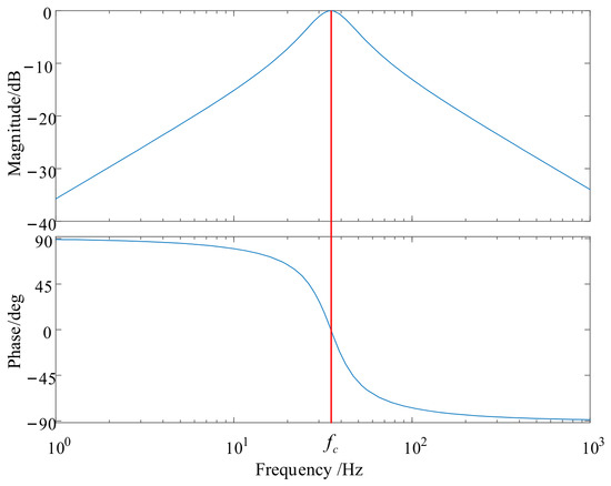
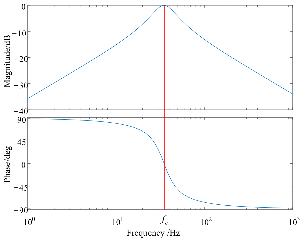
The frequency response of the SDC is shown in Figure 6. The controller has the maximum gain at the center frequency f_c, where no additional phase shift is introduced. Therefore, the oscillatory voltage component around f_c can be fed back with an appropriate damping effect. However, the gain decreases rapidly when the oscillation frequency moves away from f_c. As a result, a fixed-parameter SDC is effective only when the dominant oscillation frequency remains close to the preset center frequency.

Figure 6. Bode diagram of the supplementary damping controller.

The SVG modulation signals after introducing the supplementary damping controller are given by

$$\left\{\begin{array}{l}{m}_{ds}=(i_{drefs}-i_{ds})H_{is}(s)-K_d{i}_{qs}-H_F(s)v_{ds}\\ m_{qs}=(i_{qrefs}-i_{qs})H_{is}(s)+K_d{i}_{ds}-H_F(s)v_{qs}\end{array}\right.$$

(13)

where m_ds and m_qs are the d- and q-axis modulation signals of the SVG, i_dref,s and i_qref,s are the d- and q-axis current references, i_ds and i_qs are the SVG output currents, v_ds and v_qs are the d- and q-axis PCC voltages, H_is(s) is the SVG inner current-loop controller, and K_d is the cross-decoupling coefficient.

The SDC parameters are tuned according to the following procedure. First, the potential negative-damping frequency band is identified through the impedance-based stability analysis in Section 2. Then, the center frequency f_c is set equal to the dominant oscillation frequency identified by the VMD–Prony algorithm. The bandwidth parameter ω_b is selected to cover the expected frequency-estimation error and small frequency drift while avoiding excessive amplification outside the target oscillation band. The resonant gain K_R is selected by considering both the required phase-margin improvement and the SVG current-capacity constraint. A larger K_R provides stronger damping but may increase the supplementary current demand and affect the SVG reactive-power regulation. Therefore, K_R should be chosen to ensure sufficient damping margin without violating the SVG current limit.

In the proposed adaptive scheme, f_c is updated online according to the identified dominant oscillation frequency. To prevent frequent switching caused by measurement noise or small estimation fluctuations, a frequency deadband and a smoothing process can be introduced when updating f_c. The supplementary damping signal is activated only when a significant oscillatory component is detected; otherwise, the damping channel remains inactive and does not affect the steady-state operation of the SVG.

3.2. Oscillatory Mode Identification Based on VMD–Prony Algorithm

The Prony algorithm can estimate the frequency, amplitude, phase, and attenuation factor of oscillatory modes. However, its identification accuracy is sensitive to noise. In practical PV-integrated distribution networks, the measured PCC voltage or current signal usually contains background noise, switching-frequency components, and non-oscillatory disturbances. Directly applying Prony analysis to noisy signals may therefore lead to inaccurate modal estimation.

To improve the robustness of oscillation-mode identification, VMD is first used to decompose the measured signal into a set of band-limited intrinsic mode functions (IMFs). Noise-dominated components are then removed according to the Pearson correlation coefficient. The reconstructed denoised signal is finally processed by the Prony algorithm to extract the dominant oscillation mode. This VMD–Prony combination improves the frequency-identification accuracy under noisy conditions and provides reliable input information for adaptive damping control.

3.2.1. VMD-Based Signal Preprocessing

Variational mode decomposition decomposes a measured signal into several band-limited modal components by solving a constrained variational optimization problem. Compared with empirical mode decomposition, VMD has a more solid mathematical foundation and better mode-separation capability, which makes it suitable for extracting oscillatory components from noisy power-system signals.

The measured signal f(t) is decomposed into K modal components u_k(t), each with a center angular frequency ω_k. The constrained variational problem is formulated as:

$$\left\{\begin{array}{l}\underset{\left\{u_k\right\},\left\{{\omega }_k\right\}}{\min }\left\{{\displaystyle \sum _k||{\partial }_t\left[\left(\delta \left(t\right)+\frac{j}{\pi t}\right)u_k\left(t\right)\right]e^{-j{\omega }_{k}t}|{|}_2^2}\right\}\\ s.t.{\displaystyle \sum _k{u}_k\left(t\right)=f\left(t\right)}\end{array}\right.$$

(14)

where u_k ={u₁, u₂, …, u_K} represents the set of modal components, ω_k = {ω₁, ω₂, …, ω_K} represents the corresponding center angular frequencies.

By introducing the quadratic penalty factor α and the Lagrange multiplier operator λ(t), the constrained problem is transformed into the following unconstrained optimization problem:

$$\begin{array}{l}L\left(\left\{u_k\right\},\left\{{\omega }_k\right\},\lambda \right)=\alpha {\displaystyle \sum _k||}{\partial }_t\left[\left(\delta \left(t\right)+{\displaystyle \frac{j}{\pi t}}\right)\ast u_k\left(t\right)\right]e^{-j{\omega }_{k}t}{||}_2^2+\\ ||f\left(t\right)-{\displaystyle \sum _k{u}_k\left(t\right)|{|}_2^2}+<\lambda \left(t\right),f\left(t\right)-{\displaystyle \sum _k{u}_k}\left(t\right)>\end{array}$$

(15)

The iterative formula for initializing component signals ${\widehat{u}}_k^1$, center frequency ${\widehat{\omega }}_k^1$, ${\widehat{u}}_k^1$ and ${\omega }_k^{n+1}$ are as follows $u_k^{n+1}$:

$${\widehat{u}}_k^{n+1}(\omega )={\displaystyle \frac{\widehat{f}(\omega )-{\displaystyle \sum _i{\widehat{u}}_i(\omega )+\frac{\widehat{\lambda }(\omega )}{2}}}{1+2\alpha {(\omega -{\omega }_k)}^2}}$$

(16)

$${\omega }_k^{n+1}={\displaystyle \frac{{\displaystyle {\int }_0^{\infty }\omega |{\widehat{u}}_k(\omega ){|}^2\mathrm{d}\omega }}{{\displaystyle {\int }_0^{\infty }|{\widehat{u}}_k(\omega ){|}^2\mathrm{d}\omega }}}$$

(17)

Update Lagrange multipliers:

$${\lambda }^{n+1}(\omega )={\lambda }^n(\omega )+\tau (f(\omega )-{\displaystyle \sum _k{u}_k^{n+1}(\omega )})$$

(18)

where n is the iteration index, and τ is the noise-tolerance parameter. The iteration stops when the convergence criterion is satisfied:

$${\displaystyle \sum _k\frac{{‖{\widehat{u}}_k^{n+1}-u_k^n‖}_2^2}{{‖{\widehat{u}}_k^n‖}_2^2}<\epsilon }$$

(19)

After all IMF components are obtained, the Pearson correlation coefficient between each modal component u_k(t) and the original signal f(t) is calculated according to Appendix A Equation (A6). Modal components with weak correlation to the original signal are regarded as noise-dominated components and removed. In this paper, components with r < 0.2 are discarded. The remaining components are reconstructed to obtain a denoised signal for subsequent Prony analysis.

The VMD parameters were selected by considering the spectral composition of the sampled signal, modal-separation quality, denoising performance, and computational burden. The number of modes K determines the number of extracted intrinsic mode functions (IMFs). If K is too small, different spectral components may be mixed in the same IMF, resulting in under-decomposition. Conversely, an excessively large K may produce redundant modes or mode splitting, which increases the computational burden and may introduce false modes into the subsequent Prony analysis.

In weak-grid PV systems, the measured PCC voltage or current signal usually contains the fundamental-frequency component, coupled sub-/super-synchronous oscillatory components, and residual noise. Due to frequency coupling introduced by converter control loops and PLL dynamics, an oscillatory interaction may appear as a pair of sideband components around the fundamental frequency, such as f₁ − Δf and f₁ + Δf. Therefore, K = 4 was selected in this work to separate the fundamental or fundamental-related component, the main coupled oscillatory components, and one residual/noise-dominated component. The known fundamental component is not used for damping-controller tuning; only the dominant oscillatory mode identified after VMD-based preprocessing and Prony analysis is used to update the SDC center frequency.

The penalty factor α controls the bandwidth of each modal component. A small α may lead to mode mixing, whereas an excessively large α may over-narrow the modal bandwidth and cause useful oscillatory information to be lost. Therefore, α = 2000 was adopted to balance modal separation and signal reconstruction accuracy. The convergence tolerance ε determines the stopping condition of the iterative process. A loose tolerance may terminate the iteration before the center frequencies converge, whereas an overly strict tolerance increases the number of iterations with limited improvement in identification accuracy. Accordingly, ε = 1 × 10⁻⁶ was selected as a compromise between convergence accuracy and computational time.

After VMD decomposition, the Pearson correlation coefficient between each IMF and the original signal is calculated. Components with r < 0.2 are regarded as weakly correlated residual or noise-dominated components and are removed before Prony analysis. With the selected parameters K = 4, α = 2000, and ε = 1 × 10⁻⁶, the VMD–Prony method achieves effective denoising and modal separation in the tested cases. The same parameter settings are used in the subsequent simulation studies unless otherwise specified.

3.2.2. Prony-Based Modal Identification

After VMD-based denoising, the reconstructed signal is processed by the Prony algorithm to estimate the modal parameters. The Prony algorithm approximates the sampled signal as a linear combination of exponentially damped sinusoidal components. The mathematical model is expressed as:

$$\widehat{x}\left(n\right)={\displaystyle \sum _{i=1}^p{b}_i{z}_i^n},n=0,1,2\cdots ,N-1$$

(20)

where $\widehat{x}\left(n\right)$ is the fitting value of the sampled signal x(n); A_i, f_i, θ_i and α_i represent the amplitude, frequency, initial phase, and attenuation factor of the i-th mode, respectively; and $\Delta t$ is the sampling interval.

Equation (20) can be transformed into a homogeneous difference equation:

$$\widehat{x}\left(n\right)=-{\displaystyle \sum _{i=1}^p{a}_i}\widehat{x}\left(n-i\right)$$

(21)

The corresponding characteristic polynomial is

$$a_0{z}^p+a_1{z}^{p-1}+\cdots +a_{p-1}z+a_p=0, a_0=1$$

(22)

The fitting error is defined as

$$e\left(n\right)=x\left(n\right)-\widehat{x}\left(n\right)$$

(23)

By combining Equations (18) and (20), the following autoregressive representation can be obtained:

$$x\left(n\right)=-{\displaystyle {\displaystyle \sum _{i=1}^p}{a}_{k}x\left(n-k\right)+}{\displaystyle {\displaystyle \sum _{i=0}^p}{a}_{k}e\left(n-k\right)}$$

(24)

Define noise

$$\epsilon \left(n\right)={\displaystyle \sum _{i=0}^p{a}_{k}e\left(n-k\right)},\left(n=0~N-1\right)$$

(25)

Then (24) becomes

$$x\left(n\right)=-{\displaystyle \sum _{i=1}^p{a}_{i}x\left(n-i\right)}+\epsilon \left(n\right)$$

(26)

Equation (26) can be seen as the noise ε(n) exciting the output of a p-order autoregressive (AR) model. The coefficients of the differential equation to be solved are the parameters a_i of the AR model, and the canonical equation of the AR model is:

$$\left[\begin{array}{cccc}r(1,0)& r(1,1)& \cdots & r(1,p)\\ r(2,0)& r(2,1)& \cdots & r(2,p)\\ ⋮& ⋮& ⋮& ⋮\\ r(p,0)& r(p,1)& \cdots & r(p,p)\end{array}\right]\left[\begin{array}{c}{a}_0\\ a_1\\ ⋮\\ a_p\end{array}\right]=\left[\begin{array}{c}{u}_p\\ 0\\ ⋮\\ 0\end{array}\right]$$

(27)

where

$$u_p={\displaystyle \sum _{i=0}^p{a}_i\left[{\displaystyle \sum _{n=p}^{N-1}x\left(n-i\right)x^{\ast }\left(n\right)}\right]}$$

(28)

$$r\left(k,j\right)={\displaystyle \sum _{n=p}^{N-1}x\left(n-j\right)}{x}^{\ast }\left(n-k\right)$$

(29)

According to (26), the sample matrix R can be constructed as:

$${\mathrm{R}}_{p_1\times (p_1+1)}=\left[\begin{array}{cccc}r\left(1,0\right)& r\left(1,1\right)& \cdots & r\left(1,p_1\right)\\ r\left(2,0\right)& r\left(2,1\right)& \cdots & r\left(2,p_1\right)\\ ⋮& ⋮& ⋮& ⋮\\ r\left(p_1,0\right)& r\left(p_1,1\right)& \cdots & r\left(p_1,p_1\right)\end{array}\right]$$

(30)

where p₁ is the total number of singular value decompositions. To determine the effective order of R, perform singular value decomposition on it and sort the obtained singular values as follows:

$${\sigma }_1\ge {\sigma }_2\ge {\sigma }_m\ge {\sigma }_{m+1}\approx \dots \approx {\sigma }_{p_1}$$

(31)

where σ_m is the m singular value. Performing second-order differential calculations on the singular values mentioned above

$${\nabla }^2\sigma \left(m\right)=\sigma \left(m\right)-2\sigma \left(m-1\right)+\sigma \left(m-2\right)$$

(32)

where when the value of m increases towards the initial order p₁, and the value of $|\nabla \sigma \left(m\right)|$ gradually decreases to 0, the corresponding value of m is the critical point between noise and effective order, which is the practical order p. The effective order p is determined according to the variation trend of the singular values. The point at which the second-order difference gradually approaches zero is regarded as the boundary between effective oscillatory modes and noise-dominated modes. After p is determined, the autoregressive coefficients are obtained, and the roots of the characteristic polynomial are calculated. The modal parameters, including attenuation factor, frequency, amplitude, and initial phase, are then obtained as

$$\left\{\begin{array}{l}{\alpha }_i={\displaystyle \frac{\ln \left|z_i\right|}{\Delta t}}\\ f_i=\arctan {\displaystyle \frac{\mathrm{Im}\left(z_i\right)/\mathrm{Re}\left(z_i\right)}{2\pi \Delta t}}\\ A_i=\left|b_i\right|\\ {\phi }_i=\arctan {\displaystyle \frac{\mathrm{Im}\left(b_i\right)}{\mathrm{Re}\left(b_i\right)}}\end{array}\right.$$

(33)

The dominant oscillation mode is selected according to modal amplitude, damping ratio, and frequency location. Its frequency is denoted as f_id and is used as the input for adaptive tuning of the SDC center frequency.

3.3. Oscillation Suppression Using SVG-Based Adaptive Supplementary Damping Control

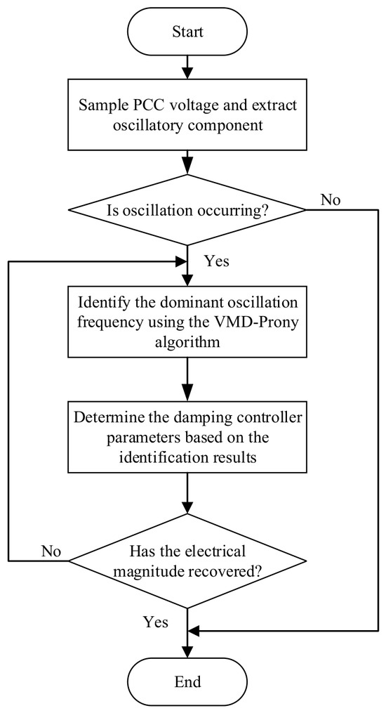
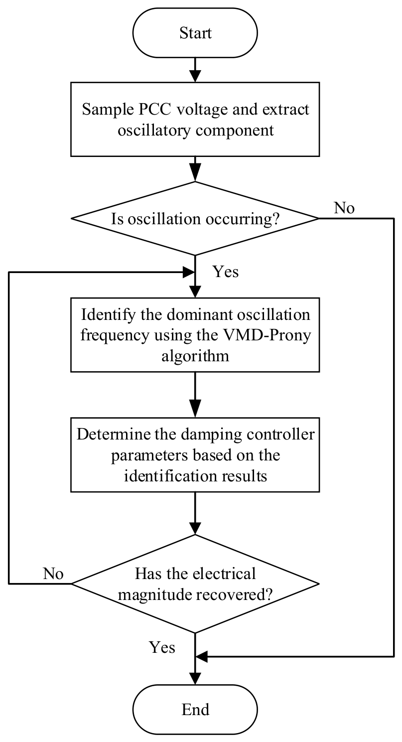
Based on the supplementary damping controller and the VMD–Prony modal identification method, the proposed adaptive suppression procedure is shown in Figure 7. The procedure contains four main stages: signal monitoring, modal identification, adaptive parameter updating, and damping control.

Figure 7. Flowchart of the proposed SVG-based adaptive supplementary damping control method.

First, the PCC voltage signal is sampled, and its oscillatory component is extracted. The VMD–Prony algorithm is then used to identify the dominant oscillation frequency. If no significant oscillation mode is detected, the supplementary damping channel remains inactive, and the SVG continues its normal reactive-power regulation without introducing additional control action.

Once a significant oscillation mode is detected, the controller enters the adaptive adjustment stage. The identified dominant frequency f_id is used to update the center frequency f_c of the supplementary damping controller. The controller then generates a compensating damping signal through the voltage-feedback channel. This signal reshapes the equivalent impedance of the SVG-integrated PV plant and increases the damping in the critical oscillation band.

After the oscillatory component decays and the electrical variables return to a stable range, the controller returns to the monitoring stage. In this manner, the proposed method can adaptively respond to changes in grid strength, converter control parameters, and oscillation frequency.

The specific procedure is summarized as follows:

(1)

Sample the PCC voltage signal and extract the oscillatory component.

(2)

Apply the VMD–Prony algorithm to identify the dominant oscillation frequency f_id.

(3)

Determine whether a significant oscillation mode exists according to the modal amplitude and damping characteristics.

(4)

If oscillation is detected, update the center frequency f_c of the supplementary damping controller according to f_id.

(5)

Generate the supplementary damping signal through the SVG voltage-feedback branch and suppress the oscillation by reshaping the system impedance.

(6)

After the oscillation is damped, return to the monitoring stage.

3.4. Real-Time Implementation and Computational Burden

The proposed adaptive damping strategy consists of two layers: the fast SVG current-control layer and the supervisory modal-identification layer. The SVG inner current controller and reactive-power control loop operate at their original control frequency. The VMD–Prony algorithm is implemented in the supervisory layer and is used only to update the center frequency of the supplementary damping controller. Therefore, the modal-identification algorithm does not need to run at the same frequency as the SVG inner current loop.

The computational burden of the proposed method mainly comes from VMD-based signal decomposition and Prony-based modal estimation. For a sampling window with N data points, K VMD modes, and I_max maximum VMD iterations, the computational complexity of VMD is approximately O(I_maxKNlogN) when FFT-based implementation is used. For the Prony stage, the main computational burden is associated with constructing the sample matrix and performing singular value decomposition. If p₁ is the initial Prony order, the computational complexity can be approximated as $O(N{p}_1^2+p_1^3)$.

In the simulation tests, the VMD–Prony algorithm calculates the oscillation modal information within 80 ms. This computation time is acceptable for supervisory-level adaptation of the SDC center frequency, because the adaptive update is not performed in the high-frequency inner control loop. In practical implementation, the algorithm can be triggered only when the oscillatory component exceeds a preset threshold, which further reduces the computational burden during normal steady-state operation.

To avoid control chattering caused by noise or small frequency-estimation fluctuations, the identified frequency can be processed using a deadband and rate limiter before updating f_c. In addition, the supplementary damping signal should be constrained by the available SVG current margin to prevent interference with the primary reactive-power regulation function. From an engineering perspective, the VMD–Prony algorithm can be implemented on a DSP, FPGA, or industrial real-time controller. The VMD stage can be accelerated by FFT-based computation, while the Prony stage involves only low-order matrix operations after VMD denoising. Hardware-in-the-loop validation and field implementation under measurement noise, communication delay, and SVG current saturation will be considered in future work.

4. Case Studies

4.1. Validation of the Proposed Models and Algorithms

4.1.1. Impedance Model Validation

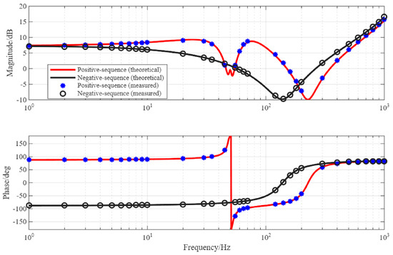
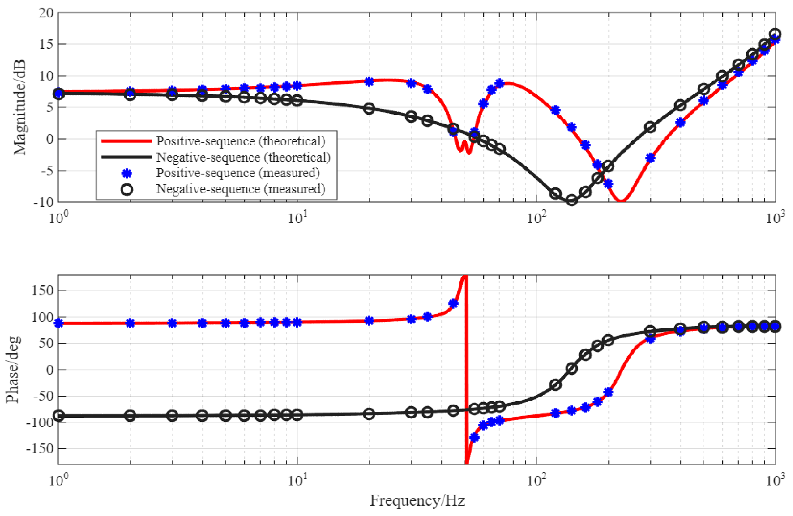
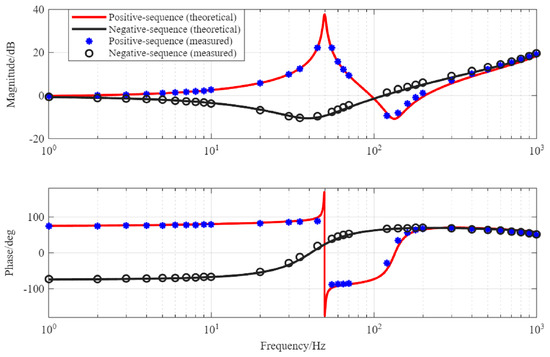
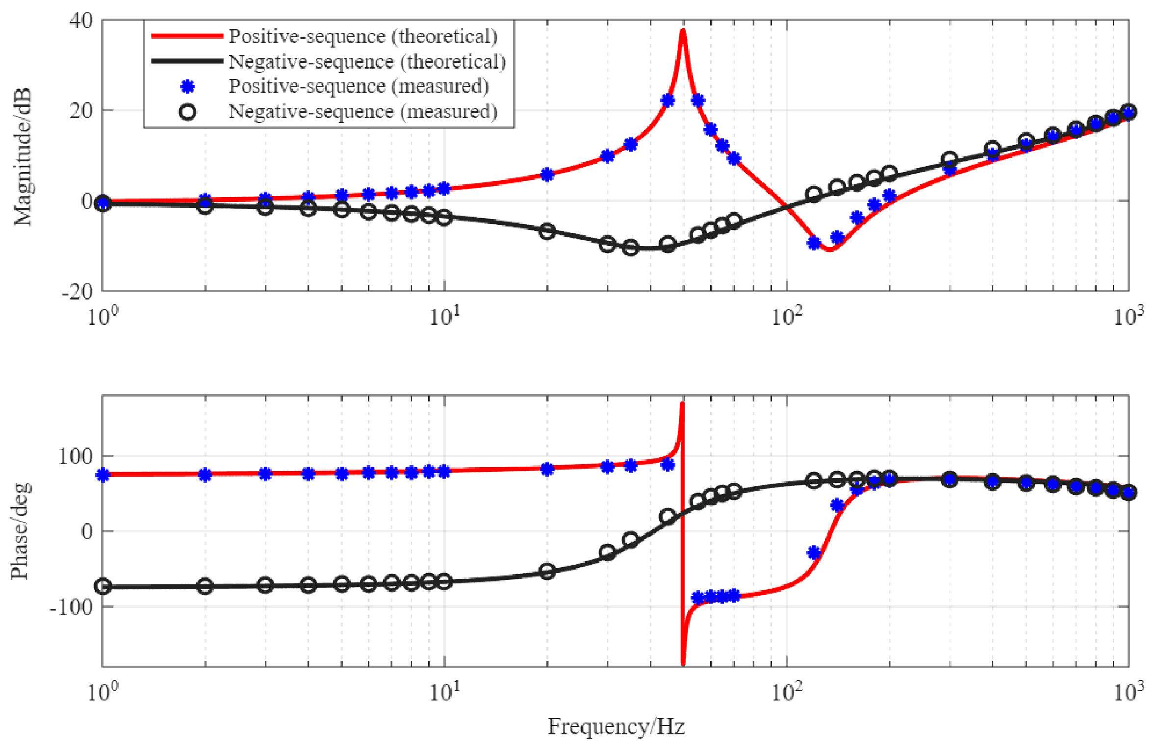
To validate the accuracy of the derived sequence-impedance models, frequency-sweep tests were performed for both the PV inverter and the SVG. The corresponding system parameters are listed in Table 1 and Table 2, and the comparison between the theoretical impedance calculation and the frequency-sweep results is shown in Figure 8 and Figure 9.

Table 1. Parameters of Photovoltaic Grid-connected System.

Parameters	Numerical Values
Filter inductor L	0.6 mH
Current inner loop PI parameters	kpi = 0.35, kii = 1000
Phase Locked Loop Parameters	kppll = 0.05, kipll = 0.25
Cross decoupling coefficient	Ksdq = 0.003
Rated capacity of each PV inverter unit	P = 1 MW

Table 2. Parameters of the grid-connected SVG.

Parameters	Numerical Values
DC capacitor Cs	10,000 μF
Filter inductance Ls	0.0001 H
Current inner loop PI parameters	kpis = 0.15, kiis = 200
PI parameters of phase-locked loop	kpplls = 0.25, kiplls = 10
Reactive power outer loop PI parameters	kpQs = 0.00012, kiQs = 0.003
Cross decoupling coefficient	ksdq = 0.0048
SVG capacity	Q = 1 MVar

Figure 8. Comparison between the calculated and swept sequence impedances of the PV inverter.

Figure 9. Comparison between the calculated and swept sequence impedances of the SVG.

As shown in Figure 8, the calculated positive- and negative-sequence impedances of the PV inverter agree well with the frequency-sweep results over the studied frequency range. Similarly, Figure 9 shows that the theoretical SVG impedance model accurately captures the measured magnitude and phase characteristics. The good agreement between the analytical results and the sweep results verifies the correctness of the proposed sequence-impedance models. Therefore, the established impedance models can provide a reliable basis for subsequent stability analysis, oscillation-mechanism investigation, and damping-controller design in the SVG-integrated PV plant.

4.1.2. Validation of the Impedance-Reshaping Effect of the SVG Supplementary Damping Controller

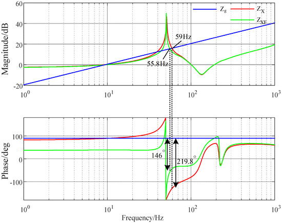
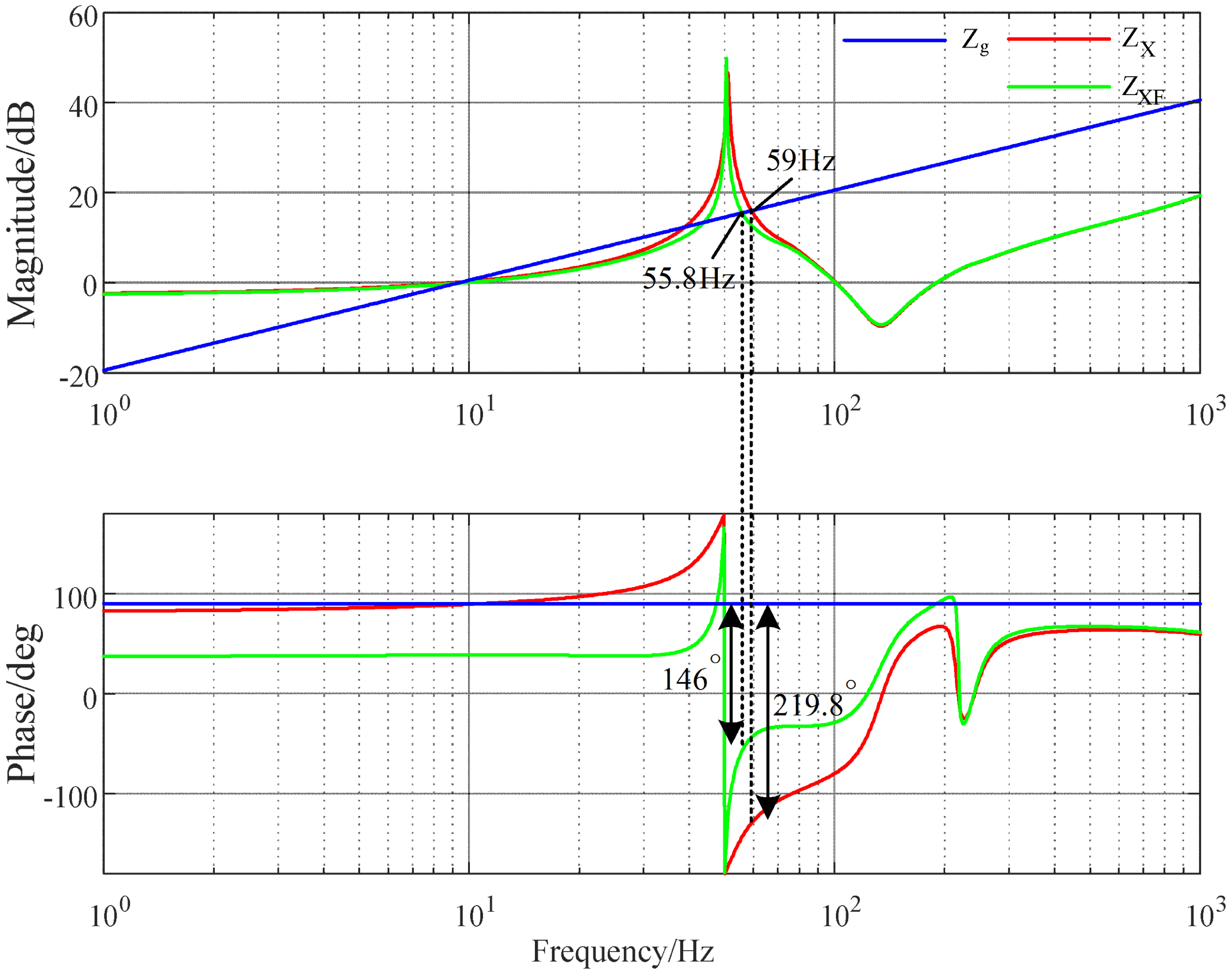
Using the parameters listed in Table 1 and Table 2, the aggregated impedance of the PV plant with the SVG supplementary damping controller can be calculated by incorporating the SVG supplementary damping controller in Equations (12) and (13) into the plant-level impedance model. Figure 10 compares the impedance characteristics of the PV plant before and after the supplementary damping controller is introduced.

Figure 10. Impedance characteristics of the PV plant before and after applying the SVG supplementary damping controller.

Without supplementary damping control, the phase margin at the impedance intersection frequency is −39.8°, indicating that the interaction between the PV plant impedance and the weak-grid impedance may cause instability. After the SVG supplementary damping controller is applied, the capacitive negative-damping characteristic in the sub-/super-synchronous frequency band is significantly mitigated. The phase margin at the impedance intersection frequency is increased to 34°, which satisfies the impedance-based stability criterion. These results confirm that the proposed SVG supplementary damping controller can reshape the system impedance and enhance the damping margin in the critical oscillation frequency band.

4.1.3. Validation of the VMD–Prony Modal Identification Method

To evaluate the accuracy and noise robustness of the proposed VMD–Prony modal identification method, an ideal oscillatory signal is constructed as follows:

$$\begin{array}{l}y\left(t\right)=3.6e^{-0.3t}\cos (2\pi \times 32.5t+\pi /4)+2.1e^{-0.6t}\cos (2\pi \times 47.3t-\pi /6)+\\ 1.5e^{0.4t}\cos (2\pi \times 67.9t+\pi /5)\end{array}$$

(34)

A 20 dB Gaussian white noise component is added to the ideal signal. The sampling duration is 1 s, and the sampling frequency is 500 Hz. First, the conventional Prony method is directly applied to the noisy signal y₁(t), and the identification results are listed in Table 3. The results show that the conventional Prony method is sensitive to noise, resulting in noticeable frequency-identification errors and inaccurate damping estimation.

Table 3. Modal identification results obtained using the conventional Prony method under noisy conditions.

Modal	Amplitude	Frequency/Hz	Attenuation Factor	Damping Ratio
1	3.32	30.298	−0.37599	0.00198
2	1.83	48.83	−0.78608	0.00256
3	1.75	66.06	0.46288	−0.00111

To improve the robustness of modal identification, the noisy signal is preprocessed using VMD before Prony analysis. The denoising performance of VMD is compared with that of wavelet threshold denoising (WTD) and empirical mode decomposition (EMD), as shown in Table 4. Compared with WTD, VMD reduces the root mean square error (RMSE) from 0.116 to 0.0563 and increases the signal-to-noise ratio (SNR) from 27.715 dB to 33.968 dB. These results indicate that VMD provides better denoising performance and preserves the dominant oscillatory components more effectively.

Table 4. Algorithms Comparison of denoising performance among EMD, WTD, and VMD.

Evaluation Metric	EMD Algorithm	WTD Algorithm	VMD Algorithm
RMSE	0.1934	0.116	0.0563
SNR	23.255	27.715	33.968

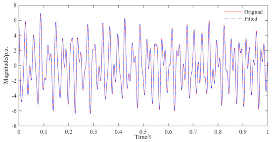
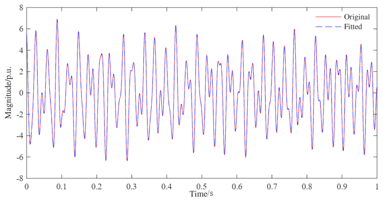
After VMD-based denoising, the reconstructed signal is processed by the Prony algorithm. The identification results are shown in Table 5. Compared with the results in Table 3, the VMD–Prony method provides more accurate modal frequency estimation and damping-factor identification. The identified modal frequencies are 32.509 Hz, 47.282 Hz, and 67.909 Hz, which are close to the actual oscillatory components of the constructed signal. Figure 11 further compares the ideal signal and the fitted signal obtained using the VMD–Prony method. The fitted signal agrees well with the ideal signal, confirming the effectiveness of the proposed modal identification method under noisy conditions.

Table 5. Modal identification results obtained using the VMD–Prony method under noisy conditions.

Modal	Amplitude	Frequency/Hz	Attenuation Factor	Damping Ratio
1	3.6	32.509	−0.3033	0.001487
2	2.16	47.282	−0.60793	0.002045
3	1.49	67.909	0.40936	−0.000962

Figure 11. Comparison between the ideal signal and the fitted signal obtained using the VMD–Prony method.

In addition, the computation time of the VMD–Prony algorithm is evaluated in the simulation environment. The algorithm can calculate the oscillation modal information within 80 ms, which is acceptable for supervisory-level adaptive tuning of the SVG damping controller.

4.2. Simulation Verification of Oscillation-Suppression Performance

4.2.1. Oscillation Suppression Under Different Operating Conditions

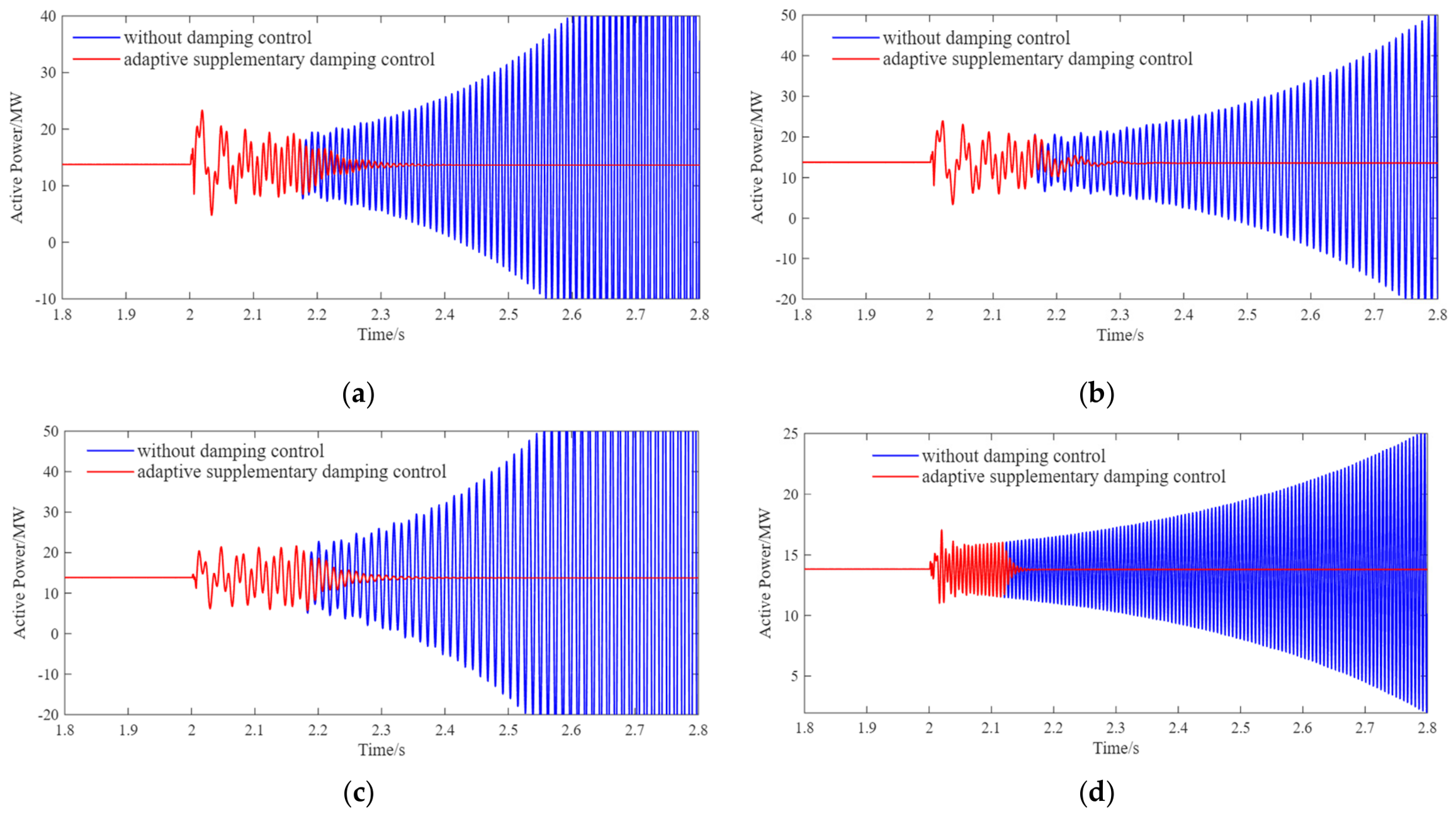
An electromagnetic transient simulation model of the SVG-integrated PV plant shown in Figure 1 is developed in MATLAB/Simulink to verify the oscillation-suppression performance of the proposed adaptive supplementary damping control method. At the beginning of the simulation, the short-circuit ratio (SCR) is set to 4. At t = 2 s, the grid impedance is increased to reduce the SCR and induce sub-/super-synchronous oscillations. Four operating conditions are designed to produce oscillations with different dominant frequencies, as listed in Table 6. Condition 1 uses the system parameters listed in Table 1 and Table 2, whereas Conditions 2–4 are obtained by adjusting the SVG current-loop and PLL parameters while maintaining stable pre-disturbance operation.

Table 6. Parameters and dominant oscillation frequencies under four operating conditions.

Operating Condition	His(s)	Hplls(s)	SCR	Main Oscillation Frequency/Hz
1	0.15 + 200/s	0.25 + 10/s	2.3	57
2	0.15 + 200/s	0.05 + 10/s	2.7	45
3	0.1 + 150/s	0.05 + 0.5/s	2.1	35
4	0.33 + 1000/s	0.05 + 0.5/s	2.9	115

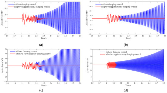
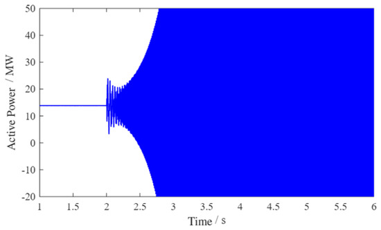
As shown in Figure 12, when no damping measure is applied, the active power of the PV plant exhibits severe oscillations after the SCR decreases. The oscillation amplitude increases rapidly, indicating that the system loses damping under weak-grid conditions. The dominant oscillation frequency varies with the operating condition, ranging from 35 Hz to 115 Hz, which confirms that the oscillation mode is strongly affected by controller parameters and grid strength.

Figure 12. Oscillation-suppression performance of the proposed ASDC under different operating conditions: (a) Condition 1, 57 Hz; (b) Condition 2, 45 Hz; (c) Condition 3, 35 Hz; (d) Condition 4, 115 Hz.

After the proposed ASDC is activated, the dominant oscillation frequency is identified online using the VMD–Prony algorithm, and the center frequency of the SVG supplementary damping controller is updated accordingly. In all four operating conditions, the active-power oscillation is rapidly attenuated, and the system returns to a stable operating state. These results demonstrate that the proposed ASDC can adapt to oscillations with different dominant frequencies and provide effective damping over a wide frequency range.

4.2.2. Comparison Between Fixed-Parameter SDC and the Proposed ASDC Under SCR Variation

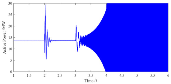
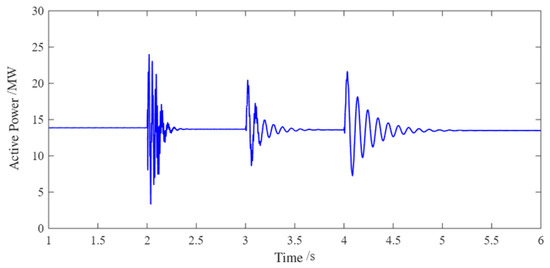
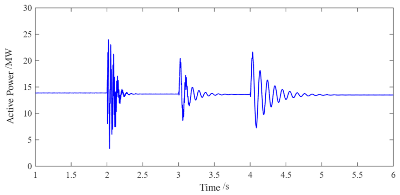
To further verify the adaptability of the proposed ASDC, the system parameters corresponding to Condition 2 are used, and the SCR is sequentially reduced from 4 to 2.7, 2.4, and 2.1 at t = 2 s, t = 3 s, and t = 4 s, respectively. Three cases are compared: the system without damping control, the system with fixed-parameter supplementary damping control (SDC), and the system with the proposed ASDC. The center frequency of the fixed-parameter SDC is set to 45 Hz, which corresponds to the dominant oscillation frequency when SCR = 2.7. The simulation results are shown in Figure 13, Figure 14 and Figure 15.

Figure 13. Active-power response of the PV plant without damping control under sequential SCR reduction.

Figure 14. Active-power response of the PV plant using fixed-parameter SDC under sequential SCR reduction. The controller suppresses the oscillation when SCR = 2.7 but fails when the oscillation frequency shifts under lower SCR conditions.

Figure 15. Active-power response of the PV plant using the proposed ASDC under sequential SCR reduction. The ASDC maintains stable operation by adaptively updating the damping-controller center frequency.

As shown in Figure 13, when no damping controller is used, the PV plant output power diverges after the SCR decreases, indicating that the weak-grid interaction leads to unstable oscillation. Figure 14 shows the response obtained using the fixed-parameter SDC. When SCR = 2.7, the dominant oscillation frequency is close to the preset center frequency of 45 Hz, and the fixed-parameter SDC can suppress the oscillation effectively. However, when SCR further decreases to 2.4, the oscillation frequency shifts away from the preset center frequency. As a result, the damping effect of the fixed-parameter SDC deteriorates, and the active-power oscillation begins to diverge. When SCR decreases to 2.1, the grid strength is further weakened and the fixed-parameter SDC can no longer maintain system stability.

In contrast, Figure 15 shows that the proposed ASDC maintains effective oscillation suppression during the entire SCR variation process. This is because the VMD–Prony algorithm identifies the dominant oscillation frequency online, and the center frequency of the SVG damping controller is updated accordingly. Therefore, the proposed ASDC can overcome the frequency-mismatch problem of the fixed-parameter SDC and maintain stable operation under varying grid strengths.

4.3. Robustness Discussion

The robustness of the proposed ASDC is mainly determined by the accuracy of dominant-frequency identification, the bandwidth of the supplementary damping controller, and the available current margin of the SVG. Since the center frequency f_c is updated according to the identified dominant oscillation frequency, small identification errors may cause a slight mismatch between the damping-controller center frequency and the actual oscillation frequency. However, as long as the error remains within the effective bandwidth determined by ω_b, the controller can still provide sufficient positive damping. Therefore, ω_b should be selected by considering both the expected frequency-estimation error and the possible frequency drift caused by SCR variation.

The damping gain K_R also affects the robustness of the controller. A larger K_R can improve the damping effect, but it may increase the supplementary current demand of the SVG. Conversely, an excessively small K_R may lead to insufficient damping. Therefore, K_R should be selected to provide adequate damping while satisfying the SVG current-capacity constraint. In practical implementation, an amplitude limiter and an anti-windup mechanism can be introduced to prevent the damping signal from exceeding the SVG current limit.

In addition, the adaptive update of f_c should not be performed too frequently. A frequency deadband and a rate limiter can be used to avoid parameter chattering caused by noise or small identification fluctuations. These measures are expected to improve the practical robustness of the proposed ASDC under modal-identification errors, SVG parameter deviations, and operating-condition variations. A quantitative sensitivity analysis considering identification errors, SVG parameter deviations, and controller latency will be investigated in future work.

5. Conclusions

This paper proposed an SVG-based adaptive supplementary damping control strategy for mitigating wideband oscillations in PV-integrated weak-grid systems. A sequence-impedance model of the SVG-integrated PV plant was established, and the oscillation mechanism was analyzed using the Nyquist stability criterion. A VMD–Prony modal identification method was then introduced to update the center frequency of the SVG supplementary damping controller according to the identified dominant oscillation frequency. The main conclusions are as follows.

(1) The impedance-based analysis shows that the interaction between the capacitive negative-damping characteristics of the PV plant and the inductive weak-grid impedance can lead to sub-/super-synchronous oscillations. After introducing the SVG supplementary damping controller, the system impedance is effectively reshaped, and the phase margin is improved from −39.8° to 34° in the tested case.

(2) The VMD–Prony method improves the accuracy of oscillation-mode identification under noisy conditions. In the 20 dB Gaussian-noise test, VMD achieves an RMSE of 0.0563 and an SNR of 33.968 dB, providing reliable frequency information for adaptive damping control.

(3) Simulation results verify that the proposed ASDC can suppress oscillations with dominant frequencies ranging from 35 Hz to 115 Hz. Compared with fixed-parameter SDC, the proposed method maintains better damping performance when the oscillation frequency shifts with changes in grid strength.

The present study is based on electromagnetic transient simulations. Future work will focus on hardware-in-the-loop validation and practical implementation considering controller latency, measurement noise, and SVG current saturation.

References

- Cespedes, M.; Sun, J. Impedance modeling and analysis of grid-connected voltage-source converters. IEEE Trans. Power Electron. 2014, 29, 1254–1261. [Google Scholar] [CrossRef] [Scilit]
- Eskandari, M.; Savkin, A.V.; Alhelou, H.H.; Blaabjerg, F. Explicit impedance modeling and shaping of grid-connected converters via an enhanced PLL for stabilizing the weak grid connection. IEEE Access 2022, 10, 128874–128889. [Google Scholar] [CrossRef] [Scilit]
- Wang, S.; Zhou, G.; Hao, P.; Chen, J. Designing parameters to reshape the inverter output impedance based on the D-split method under weak grid conditions. Electronics 2023, 12, 5000. [Google Scholar] [CrossRef] [Scilit]
- Yang, D.; Wang, X.; Liu, F.; Xin, K.; Liu, Y.; Blaabjerg, F. Symmetrical PLL for SISO impedance modeling and enhanced stability in weak grids. IEEE Trans. Power Electron. 2020, 35, 1473–1483. [Google Scholar] [CrossRef] [Scilit]
- Li, P.; Xiong, L.; Wang, Z.; Ma, M.; Wang, J. Fractional-order sliding mode control for damping of subsynchronous control interaction in DFIG-based wind farms. Wind Energy 2019, 23, 749–762. [Google Scholar] [CrossRef] [Scilit]
- Pang, B.; Nian, H. Active damping technique based on H∞ controller for VSC under parallel compensation grid. Electron. Lett. 2019, 56, 2682–2691. [Google Scholar]
- Xie, Z.; Chen, Y.; Wu, W.; Gong, W.; Guerrero, J.M. Stability enhancing voltage feed-forward inverter control method to reduce the effects of phase-locked loop and grid impedance. IEEE J. Emerg. Sel. Top. Power Electron. 2021, 9, 3000–3009. [Google Scholar] [CrossRef] [Scilit]
- Li, G.; Chen, Y.; Luo, A.; Wang, H. An enhancing grid stiffness control strategy of STATCOM/BESS for damping sub-synchronous resonance in wind farm connected to weak grid. IEEE Trans. Ind. Inform. 2020, 16, 5835–5845. [Google Scholar] [CrossRef] [Scilit]
- Han, X.; Wang, H.; Wu, S.; Lyu, J.; Cai, X. A stabilization control strategy for SVG to mitigate subsynchronous oscillations caused by PMSG-based wind farms. In Proceedings of the 2025 IEEE 16th International Symposium on Power Electronics for Distributed Generation Systems (PEDG), Nanjing, China, 22–25 June 2025; IEEE: Piscataway, NJ, USA, 2025; pp. 993–998. [Google Scholar]
- Li, H.; Wang, X.; Yan, M.; Wang, J.; Wu, C. Enhanced Damping Method for Suppressing Sub-Synchronous Oscillations of Grid-Forming Permanent Magnet Synchronous Generator. Electronics 2025, 14, 4489. [Google Scholar] [CrossRef] [Scilit]
- Yang, H.; Sun, Z.; Wang, H.; Wang, Y.; Zhu, M.; Guo, L.; Zhou, G.; Lyu, H. Adaptive Virtual Impedance Droop Control of Parallel Inverters for Islanded Microgrids. Sensors 2025, 25, 5166. [Google Scholar] [CrossRef] [Scilit] [PubMed]
- He, G.; Wang, W.; Wang, H. Coordination control method for preventing sub/super synchronous oscillations of multi-wind farm systems. CSEE J. Power Energy Syst. 2023, 9, 1655–1665. [Google Scholar]
- Wang, L.; Truong, D.-N. Stability enhancement of DFIG-based offshore wind farm fed to a multi-machine system using a STATCOM. IEEE Trans. Power Syst. 2013, 28, 2882–2889. [Google Scholar] [CrossRef] [Scilit]
- Zhou, L.; Wu, W.; Chen, Y.; He, Z.; Zhou, X.; Huang, X.C.; Yang, L.; Luo, A.; Guerrero, J.M. Virtual positive-damping reshaped impedance stability control method for the offshore MVDC system. IEEE Trans. Power Electron. 2019, 34, 4951–4966. [Google Scholar]
- Xu, Y.; Nian, H.; Wang, T.; Chen, L.; Zheng, T. Frequency coupling characteristic modeling and stability analysis of doubly fed induction generator. IEEE Trans. Energy Convers. 2018, 33, 1475–1486. [Google Scholar] [CrossRef] [Scilit]
- Zhan, Y.; Xie, X.; Liu, H.; Liu, H.; Li, Y. Frequency-domain modal analysis of the oscillatory stability of power systems with high-penetration renewables. IEEE Trans. Sustain. Energy 2019, 10, 1534–1543. [Google Scholar] [CrossRef] [Scilit]
- Liu, H.; Xie, X.; Gao, X.; Liu, H.; Li, Y. Stability analysis of SSR in multiple wind farms connected to series-compensated systems using impedance network model. IEEE Trans. Power Syst. 2018, 33, 3118–3128. [Google Scholar] [CrossRef] [Scilit]
- Yao, J.; Wang, X.; Li, J.; Liu, R.; Zhang, H. Sub-synchronous resonance damping control for series-compensated DFIG-based wind farm with improved particle swarm optimization algorithm. IEEE Trans. Energy Convers. 2019, 34, 849–859. [Google Scholar] [CrossRef] [Scilit]
- Wu, F.; Li, X.; Ji, M.; Xie, M.; Ye, J. Virtual damping control strategy to improve anti-disturbance performance for PMSM driven electric vehicle under rough road conditions. In Proceedings of the 2021 IEEE 1st International Power Electronics and Application Symposium (PEAS), Shanghai, China, 13–15 November 2021; IEEE: Piscataway, NJ, USA, 2021. [Google Scholar]
- Zhang, C.; Kang, Z.; Li, B.; Zhang, H.; Zhu, D. Impedance-based sensitivity analysis for enhanced dynamic stability in DC off-grid hydrogen production systems. Energy Convers. Manag. X 2025, 27, 101175. [Google Scholar] [CrossRef] [Scilit]
- Kamel, H.; Dlimi, S.; Ouissaaden, F.I.; Mesbahi, O.; El Mouataouakil, A. Grid Integration of Photovoltaic Systems: Modeling, Control Strategies, and Simulation for Enhanced Performance. Results Eng. 2026, 30, 110691. [Google Scholar] [CrossRef] [Scilit]
- Zheng, C.; Yang, X.; Zhao, C. Photovoltaic Sub-Synchronous Oscillation Suppression Method Based on Model-Free Adaptive Control. Energies 2026, 19, 1977. [Google Scholar] [CrossRef] [Scilit]
- Zhang, Y.; Unruh, P.; Fischer, B.; Braun, M. Comparative Impedance Characteristic Analysis of Grid-Following and Grid-Forming Inverters. IET Renew. Power Gener. 2025, 45, 150–163. [Google Scholar]
- Kong, W.; Zhou, Y.; Li, J.; Wu, J.; Xia, J.; Lei, L. Analysis of Low-Frequency Oscillation Characteristics and Damping Enhancement Strategy for Grid-Forming PV with DC-Voltage Controller. Front. Energy Res. 2025, 13, 1623678. [Google Scholar] [CrossRef] [Scilit]
- Mu, R.; Zhang, Y.; Wan, X.; Wang, D.; Wen, T.; Zhou, Z.; Sun, L.; Yang, B. Analysis and Mitigation of Wideband Oscillations in PV-Dominated Weak Grids: A Comprehensive Review. Processes 2025, 13, 3450. [Google Scholar] [CrossRef] [Scilit]
Disclaimer/Publisher’s Note: The statements, opinions and data contained in all publications are solely those of the individual author(s) and contributor(s) and not of MDPI and/or the editor(s). MDPI and/or the editor(s) disclaim responsibility for any injury to people or property resulting from any ideas, methods, instructions or products referred to in the content. |
© 2026 by the authors. Licensee MDPI, Basel, Switzerland. This article is an open access article distributed under the terms and conditions of the Creative Commons Attribution (CC BY) license.