


Abstract
Microalgae are photosynthetic organisms that produce bioproducts of commercial interest and are efficient sequestering CO2. The monitoring and control processes are areas for improvement to increase the efficiency of its production. There are sensor options for monitoring microalgae cultures, but the vast majority rely on microcontrollers, often lacking the robustness required for applications in more demanding conditions. Also, commercial systems with industrial capabilities can fit the above purpose, but they require licensing and are expensive. Therefore, this work presents the technical details of developing an open-source platform to monitor environmental variables using Modbus industrial sensors and Python used to control the photoperiod and for measuring pH, dissolved oxygen, electrical conductivity, water and air temperatures, photosynthetic photon flux density, irradiance, and turbidity in three photobioreactors containing the microalgae Chlorella vulgaris. The resulting time series showed that the platform preserved data and had a low outlier rate. pH measurements showed that during photosynthesis, the microalgae used CO2 as their carbon source. Dissolved oxygen and culture medium temperature had an almost perfect Pearson’s anticorrelation with air-sparging. However, with aeration interruption, the correlation was , because dissolved oxygen depends on illumination, aeration, temperature, and biomass quantity, as shown in the time series.
1. Introduction
Microalgae are photosynthetic organisms that can produce complex organic compounds, biomass, and O2 using light, nutrients, and CO2 as a carbon source [1]. Some microalgae are prokaryotes (cyanobacteria), and others are eukaryotes found in marine and freshwater ecosystems [2]. Their cultivation has spread because they have a higher growth rate than higher plants, and their biochemical composition can be modified through their culture conditions [3]. Chlorella vulgaris is one of most commercially cultivated microalgae [4]. It has applications in the food industry due to its nutritional benefits, including its rich content of proteins, lipids, carbohydrates, vitamins, and minerals [5]. Chlorella vulgaris also has other applications, including cosmetics, pharmaceuticals, feedstock for aquaculture, and biofuel production, among others [6]. Chlorella vulgaris is a spherical-shaped microalgae having a diameter of 5 to 10 μm. This microorganism thrives at temperatures of 25–30 °C and at a pH of 6.5 to 9 [7]. Even though microalgae have been cultivated industrially for several decades, their production costs remain high. Among the key areas for optimizing cultivation is improving monitoring and process control, including variables such as nutrient availability, pH, dissolved oxygen, temperature, irradiance, and photoperiod [8].
Microalgae are grown in closed photobioreactors or open ponds, the former being preferred over the latter when contamination is an issue. Closed photobioreactors offer less exposure to external environmental conditions or pollution, but their operation usually results in higher costs. Real-time monitoring is a tool that might help to improve the microalgae culture conditions. Microcontroller-based technology has proved a valuable tool for monitoring water quality parameters [9,10,11,12,13,14,15,16,17]. Without many modifications, microalgae cultures have been monitored [18,19,20,21,22,23,24,25,26,27,28]. Microcontrollers have advantages over Modbus sensors. For example, there is a wider variety of sensors available, with higher sampling rates that reduce sampling times, and their cost is generally lower than that of Modbus sensors. However, they also have disadvantages. For instance, they use low logic voltage levels such as 3.3 V or 5 V, which are not compatible with the higher voltages typically used in industrial communications. This means that their integration into industrial applications would require the use of logic-level converters and different power supplies. Furthermore, communication between sensors and devices and the microcontroller is carried out using different communication protocols such as I2C (Inter-Integrated Circuit), SPI (Serial Peripheral Interface), or UART (Universal Asynchronous Receiver/Transmitter), unlike Modbus, which has a single protocol for all its devices, resulting in simpler programming. Finally, microcontroller-based sensors, in their design, typically do not account for the conditions of industrial environments, such as factories, which require durable devices and sensors that can operate in harsh environmental and electrical noise conditions [29].
Based on their output, sensors can be categorized into two types: those that provide an analog response via a voltage or current signal, and those with a digital output that requires a communication protocol for interpretation. Digital sensors typically offer advantages over analog sensors, including greater noise immunity, higher data transfer rates, and the ability to integrate them into intelligent systems. The sensors communicating via the Modbus protocol are digital and have several strengths; for example, they use an open protocol not subject to royalties, integration into existing networks is relatively easy, and RS-485 connections can reach up to 1200 m. Also, it is possible to integrate Modbus sensors and devices from different manufacturers in the same node [30]. On the other hand, most industrial devices using proprietary communication protocols have closed technology, affecting users because they can only buy devices from a single brand, which is usually expensive, and the closed technology compromises interoperability with other systems [31]. In addition, Modbus devices may be an important player in Industry 4.0 technologies [32] and can play a significant role in IoT platforms [33]. Modbus sensors can be read using commercial software such as National Instruments’ LabVIEW, which offers support and frequent updates. However, an annual license fee is required to keep the software up to date. Furthermore, it is primarily designed for Windows operating system applications.
Real-time monitoring systems for monitoring physicochemical variables have a wide range of applications across disciplines, including water quality assessment, aquaculture, limnology, and microalgae cultivation. Some important aspects to consider for their implementation are robustness, durability, measurement stability, data preservation, and a low outlier rate. Although sensor options based on microcontroller platforms like Arduino are available on the market, some do not meet the listed criteria. Therefore, this paper presents the technical details for developing a platform coded in the open-source Python software to control photoperiod and monitor physicochemical variables in microalgae cultures using industrial sensors and one controller from various manufacturers, communicating via the royalty-free Modbus RTU protocol. The prototype was triplicated and applied to cultures of Chlorella vulgaris to test its performance. The time series obtained for air temperature, water temperature, pH, dissolved oxygen concentration, photosynthetic photon flux density (PPFD), irradiance, electrical conductivity, and photoperiod control during microalgae cultivation and with distilled water show that the platform preserves data and has a low outlier rate.
Literature Review
Table 1 summarizes the literature related to Modbus devices and sensors. In general, the device acting as the client is usually a PC, programmable logic controller (PLC), or microcontroller. Table 1 shows that Modbus sensor applications include measuring physicochemical variables in greenhouses and in aquaculture and water quality systems, as well as retrieving parameters from electrical devices, such as motors.
Table 1.
Summary of literature reviews related with Modbus sensors and devices.
2. Materials and Methods
2.1. Experimental Setup
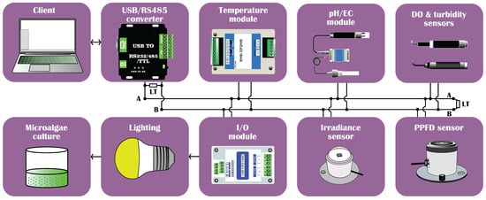
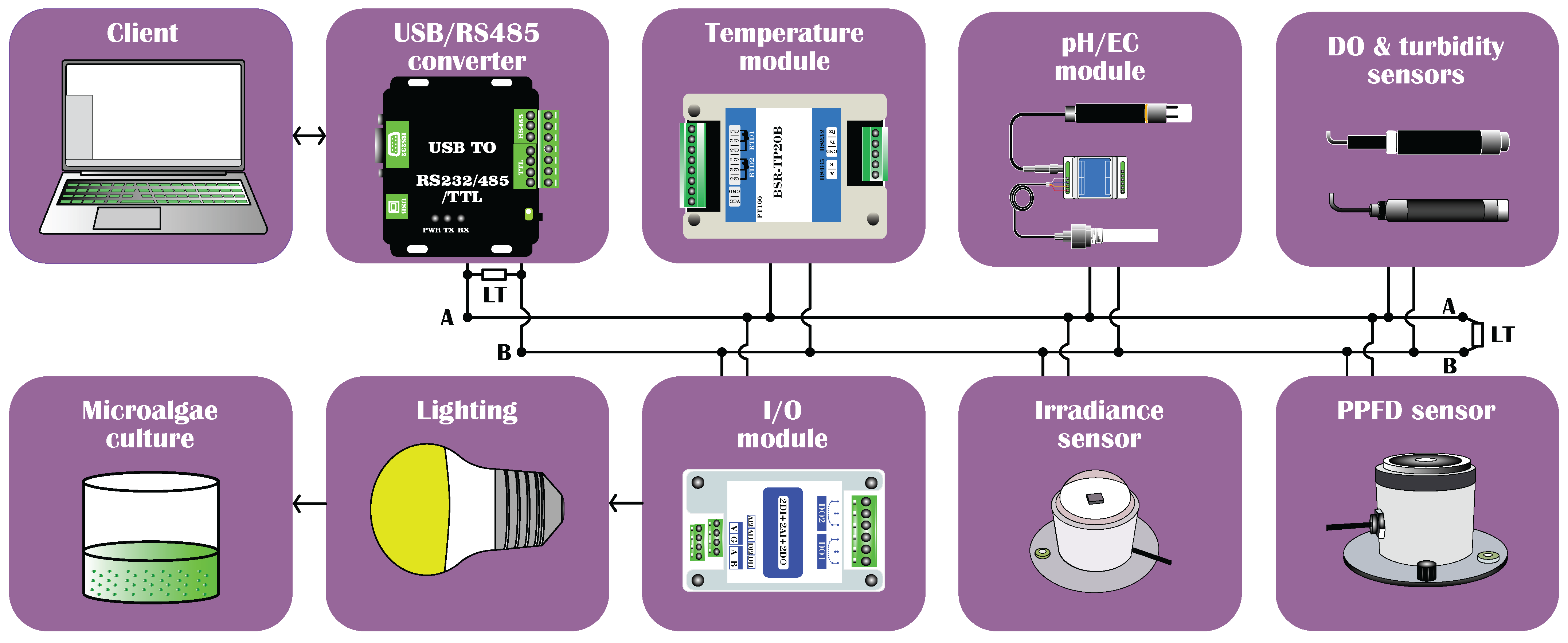
Figure 1 shows the schematic diagram of the proposed experimental setup consisting of the PC, the sensors, and the I/O device. The former assumes the client’s role in the Modbus communication. It is the only one that sends and receives messages from the rest of the Modbus sensors or modules that employ half-duplex communication [50]. The PC connects via the Universal Serial Bus (USB) to the converter, which converts the computer’s signals to the RS-485 serial communication standard. Figure 1 shows the sensors employed, of water temperature, air temperature, pH, electric conductivity, dissolved oxygen, turbidity, photosynthetic photon flux density, and irradiance, all connected using a 2-wire Modbus network with two line termination resistors of 120 Ω (LT) [51]. A Modbus module with digital and analog inputs and outputs operates a switch to control the photoperiod or the culture’s exposure to light or darkness.
Figure 1.
Schematic diagram of the experimental setup.
2.2. Modbus RTU Protocol
The Modicon company, now Schneider Electric, developed the Modbus protocol in the 1970s [50,52]. There are three variants: ASCII, RTU, and TCP/IP [52]. Modbus RTU can operate over different physical layers, such as RS-232 or RS-485 [50]. However, the RS-485 standard offers long-distance and multi-point communication, which is advantageous over the RS-232 physical layer. The architecture of a Modbus network uses a client/server (primary/secondary) communication model, in which only one client can make requests to the servers which do not communicate with each other. The servers only respond to requests from the client [30,37,39]. When using the RS-485 standard for Modbus communication, the network can have up to 32 server devices. Table 2 shows the basic configuration parameters using the RS-485 standard in Modbus RTU communication, considering that the client is a PC and that the available baud rates depend on the Modbus device [53]. Although the Modbus TCP protocol offers several advantages over the Modbus RTU protocol, such as higher data transfer rates, no limit on the number of nodes, and support for full-duplex communication, sensors and devices based on the Modbus RTU protocol are far more readily available, for example, in electronic platforms such as AliExpress and Amazon, and, above all, less expensive. This means that, in applications requiring multiple replicas, the cost is lower than that of their equivalent devices based on the Modbus TCP protocol.
Table 2.
Basic configuration parameters using the RS-485 standard in Modbus RTU communication [53].
Table 3 shows the generic message format for a Modbus RTU communication [34,37,39,53]. Each 8-bit of the message is composed of two 4-bit hexadecimal characters. The message contains 3.5 characters in the start and end parts, the address of the Modbus device acting as the server, a Modbus function code for reading or writing data, -bits of data, and a 16-bit cyclic redundancy check (CRC).
Table 3.
Generic format of a Modbus RTU message.
The Modbus protocol includes a family of functions that allow the client device to request a specific message from a server device. Table 4 shows the most common functions used in Modbus communication with most devices sold by different manufacturers. Variations in the description of the functions appear in the literature. However, those shown in Table 4 correspond to those described in the official documentation of the Python package PyModbus used in this work. The first column of the table shows the functions in decimal format, while the second column shows them in hexadecimal format.
Table 4.
Modbus function codes.
2.3. USB to RS-485 Converter and I/O Device
A generic computer does not have an interface to communicate directly through the RS-485 physical layer. Therefore, a converter is required for Modbus sensors and devices to interpret instructions from the PC. Waveshare’s industrial-grade USB-to-RS232/485/TTL converter fulfilled this role. The device also supports RS-232 communication and TTL signals. Table 5 shows some of the converter’s specifications for the RS-485 standard. This device has an internal jumper that switches to a balanced 120 Ω resistance (LT) when multiple devices are interconnected. We used the balance impedance during the experiments.
Table 5.
Main specifications of the USB to RS-485 converter.
One of the main goals of monitoring a system is to apply control actions over it. In most PLCs, control activates relays through feedback from analog or digital signals. A Modbus network can have the same capabilities. For example, in this work, the photoperiod control of the microalgae culture was performed using the MA01-AACX2220 device from China Chengdu Ebyte Electronic Technology Co., Ltd., which has two digital input channels, two analog input channels, and two relay switch outputs. Table 6 shows the device’s main characteristics.
Table 6.
Main specifications of the MA01-AACX2220 I/O device.
2.4. Modbus Sensor Selection Based on the Range of Physicochemical Variables Reported by Previous Studies in Aquaculture and Microalgae Cultivation
The selection of the sensor operating range for microalgae cultivation was based on previous reports on microalgae or aquaculture. For example, in the latter, the temperature should be between 15 and 30 °C, the pH between 6.5 and 8.5, the dissolved oxygen must exceed 5 mg/L, and the electrical conductivity must be between 200 and 2000 μS/cm [16]. The literature reports that in microalgae, the amount of photosynthetic photon flux recommended for cultures must be in the order of 100–600 μmol/m2·s [45]. In Chlorella vulgaris, the influence of dissolved oxygen on biomass production is negligible when it has values between 8 and 25 mg/L. However, when this value reaches 31 mg/L, productivity is reduced by around 30% [54]. The pH in most microalgae cultures should be below 9.5 [22]. Nephelometry has been used to estimate biomass in various microalgae species; the relationship between nephelometric turbidity units (NTU) and biomass is not linear. Studies show that this technique provides accurate measurements when turbidity is less than 1000 NTU [55,56].
Based on the measurement ranges exposed above, Table 7 shows the Modbus sensors used in this work. All of them are the RS-485 versions. The temperature module has two inputs for three-wire PT100 resistance-temperature detectors (RTDs). One served to monitor the microalgae culture, and the other measured air temperature. pH and EC used the same module to connect both electrodes. The turbidity sensor uses the 90° scattering principle. The light source comprises an infrared LED and an optical fiber for light conduction. This sensor also measures temperature. The dissolved oxygen sensor employs optical fluorescence, which requires minimal maintenance [43,57]. Illuminance or photosynthetic photon flux density are the quantities used to report radiation in microalgae cultures; PPFD more accurately reflects photosynthetic active radiation (PAR) than illuminance, because the latter uses human eye sensitivity as a standard. The selected sensor exceeds by far the 600 μmol/m2·s required for microalgae cultures as reported by Brzychczyk et al. [45]. The National Aeronautics and Space Administration (NASA) and other government agencies report irradiance to estimate the availability of solar resources in different parts of the world. The quantification of this variable might be of interest for projecting the availability of solar energy for growing microalgae outdoors at a specific geographical location; there is no need to measure it indirectly via a lux sensor [58] when the irradiance sensor is available. For the above reasons, we include this class of sensor.
Table 7.
Modbus sensors.
The sensors and the I/O device were the most expensive components of the proposed platform. The unit cost excluding taxes and shipping fees of the following items were USD 24.60 for the temperature module, USD 119.05 for the pH and EC sensors, USD 191.34 for the turbidity sensor, USD 128.45 for the dissolved oxygen sensor, USD 56.00 for the PPDF sensor, USD 49.23 for the irradiance sensor, USD 8.99 for the Module I/O, and USD 24.55 for USB to RS485 converter. All were bought through AliExpress. The cost per system was ∼USD 600. Overall, the platform is low-cost compared with the commercial alternatives.
2.5. Sensors Calibration
The temperature readings of the PT100 sensors were compared against a laboratory-grade Hg thermometer at 6, 19, and 23 °C; the relationships were linear for all sensors. The resulting calibration equations for the sensors for measuring air temperature were , , , with a correlation coefficient of 0.999, 0.985, and 0.990 for the sensors of the systems , , and , respectively. For the PT100 sensors to measure water the equations were , , , with a correlation coefficient of 0.996, 0.998, and 0.994 for the sensors of the systems , , and , respectively.
For the calibration of three pH sensors we used three standard pH solutions at 4.01, 7.01, and 10.01. The sensors showed a linear relationship with a correlation coefficient of 0.999. The calibration equations were , and , where , , and were the calibrated pH values and the magnitudes measured with the sensors for PBRs S1, S2, and S3, respectively.
To calibrate EC sensors, we compared the Modbus sensors with the Extech EC400 ExStik Conductivity/TDS/Salinity Meter using four solutions with electric conductivities of 6, 128, 280, and 560 μS/cm. The responses of the sensors were linear, and described by the equations , , and , with a correlation coefficient of 0.998, 0.99, and 0.998 for the sensors of the systems , , and , respectively.
The DO sensor was calibrated using a zero-point calibration solution and writing to the registers at address 0x1010 using the Modbus function write register (0x06) of the sensor, as indicated in the manual.
The PPFD and irradiance sensors were compared with other sensors: the NHGH09AU photosynthetically active radiation sensor from China Zhongke Nenghui Technology (Shanghai, China) and the SP-110 irradiance sensor from the USA Apogee Company (Santa Monica, CA, USA). All sensors were exposed to solar radiation for 75 min at a sampling rate of 40 s. The average values obtained were 136.73, 124.28, 127.88, and 120.28 μmol/m2·s, with standard deviations of 73.3, 85.24, 51.31, and 77.73 μmol/m2·s for the NHGH09AU sensor and the PPFD sensors from systems S1, S2, and S3, respectively. The irradiance had average values of 75.70, 89.81, 88.16, and 96.29 W/m2, with standard deviations of 38.89, 61.16, 65.9, and 56.52 W/m2 for the SP-110 sensor and the PPFD sensors of systems S1, S2, and S3, respectively. Given the upper measurement limits of irradiance and PPFD sensors, the fluctuations between them were not significant.
2.6. Software
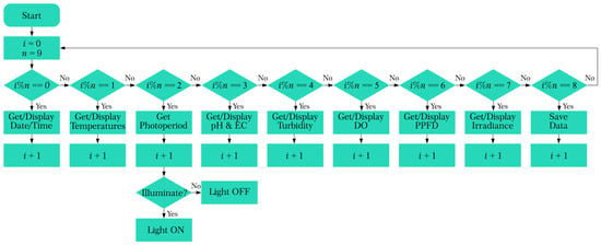
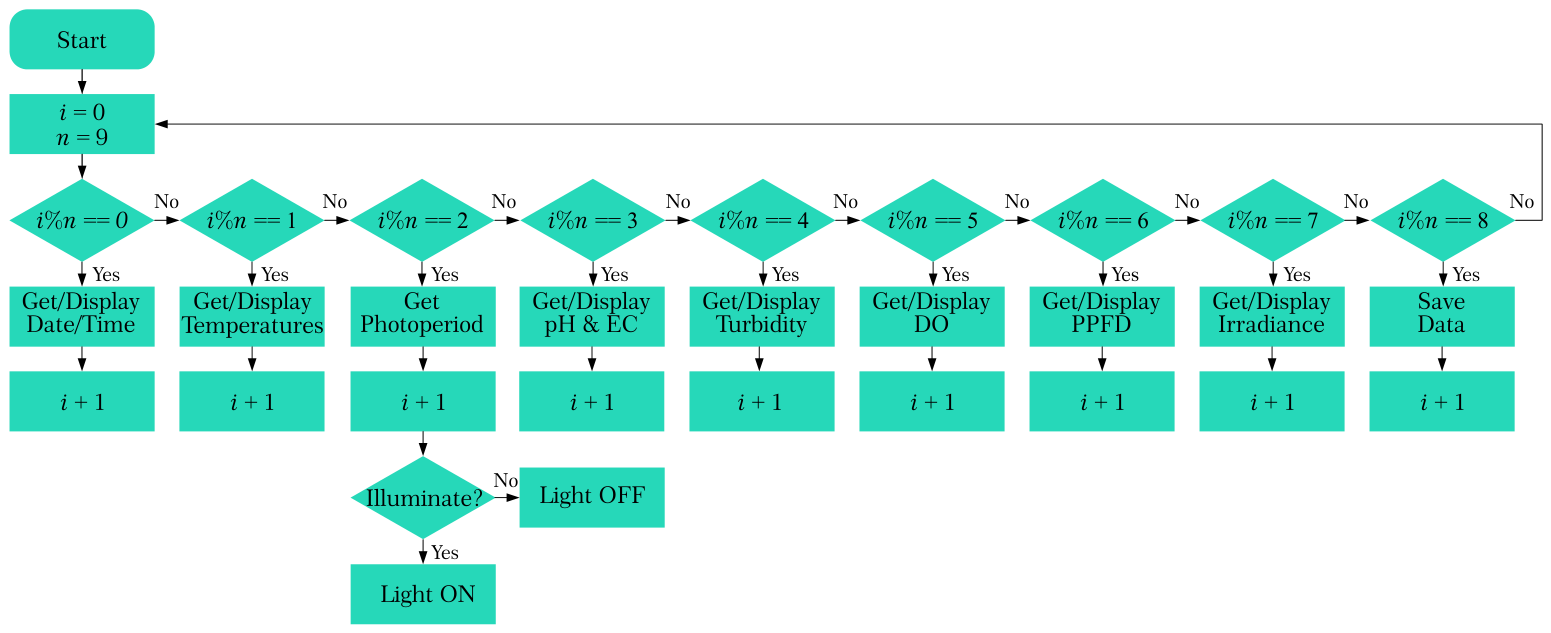
Figure 2 shows the generic flow diagram for one cycle of operation, consisting of monitoring variables and controlling the photoperiod. In this diagram, is the modulus operator, returning the remainder of a division, considering . The duration between the and events was 10 s. In one cycle, corresponds to the acquisition and display of the date and time. corresponds to the record and display of the water and air temperatures. In , the lighting is either on or off depending on the photoperiod configuration. The sequence , , , , and corresponds to the measurement and display of pH, EC, turbidity, DO, PPFD, and irradiance, respectively. At , the measurements of all variables are stored in a file with a csv extension or in a Python list, depending on the program’s operating mode: continuous or single, respectively. The total duration of one cycle, including all nine events, was 90 s (1.5 min).
Figure 2.
Flow diagram of the nine events in one cycle of monitoring and photoperiod control.
The Python platform proposed in this work required the intrinsic and third-party packages and modules shown in Table 8. The application runs in any version of Python 3.
Table 8.
Intrinsic and external Python modules and packages used in the proposed platform.
Communication between the main Python program and Modbus sensors and devices can be accomplished through several packages. For example, pyserial is one option for communicating with low-level programming [59]. Another excellent alternative is the MinimalModbus v2.1.1 package [60]. However, PyModbus v3.13.1. was selected for this work because it is a mature, complete, and well-documented package [61]. PyModbus uses a client class to communicate asynchronously or synchronously with other devices. In this work, we use the asynchronous ModbusSerialClient class.
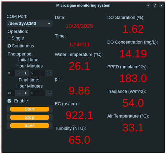
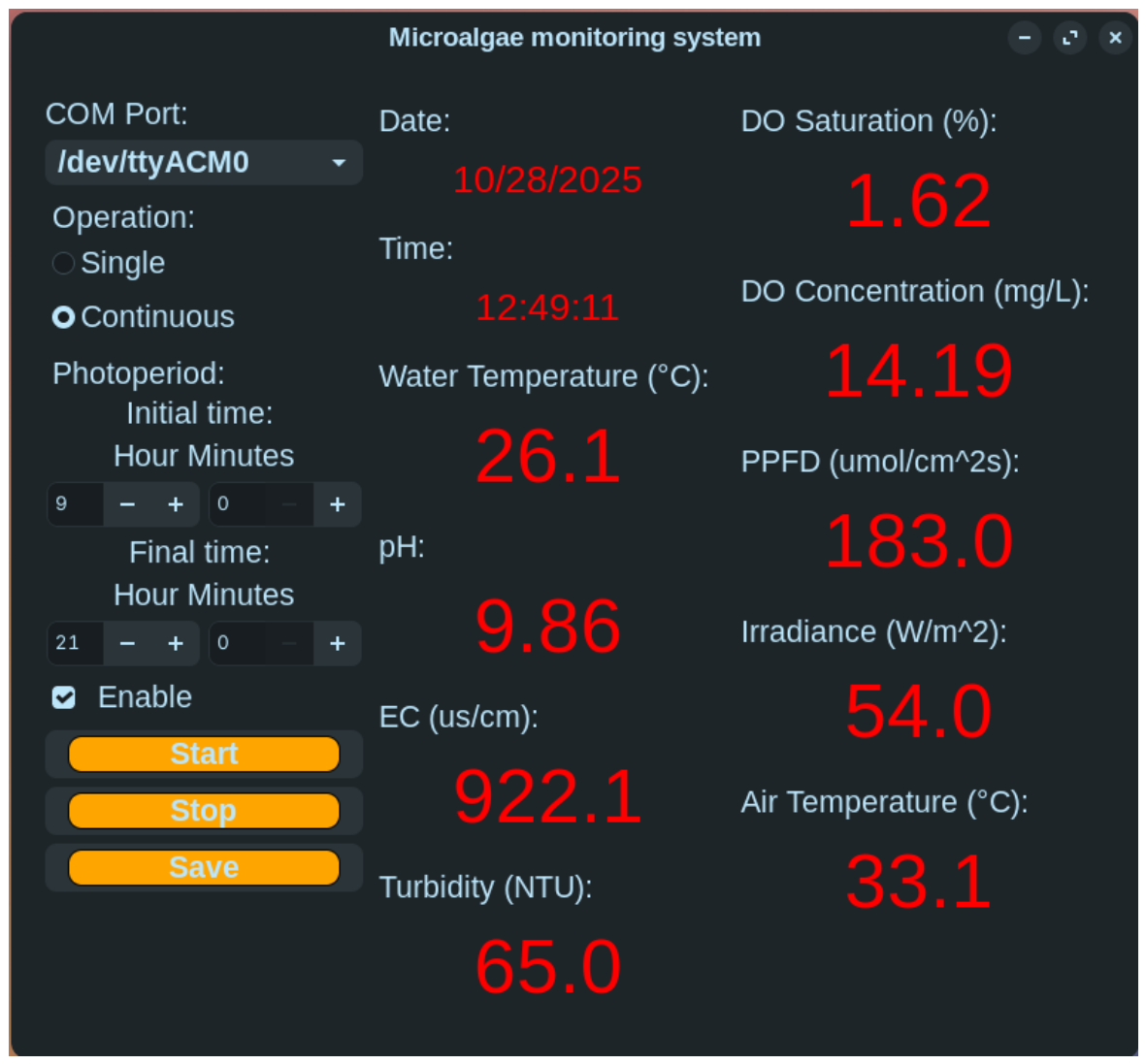
Figure 3 shows the graphical user interface (GUI) developed with the PyGobject package, which includes Python bindings to the Gtk, GLib, and Gdk libraries, as well as other libraries, to access the C library (libgtk-4.so). The dark theme of the GUI required the Adw package included in the LibAdwaita library, listed in Table 8. The GUI uses various widgets, including labels, drop-downs, buttons, frames, check buttons, and spin buttons. A drop-down widget allows selection of the serial port associated with the USB-to-RS-485 converter. A check button toggles photoperiod activation. Spin buttons set the photoperiod time. Labels display the time, date, and data from the different sensors. The GLib library’s timeout_add method allows the user to set the sampling period. Data acquisition has two operating modes: continuous, which saves data as soon as they are collected, and single, which temporarily stores data in a Python list and allows the user to save them to a file. The file format for saving data is CSV (comma-separated values).
Figure 3.
Microalgae monitoring system GUI.
Reading and writing registers in Modbus sensors and devices are not universal, as each manufacturer defines the register addresses and the Modbus functions required to transfer information. Therefore, each sensor needs its user manual. However, due to the variety of Modbus devices used in this work, we cover several situations encountered when working with them. Operating multiple Modbus devices on the same network requires different device addresses and the same baud rate. Table 9 shows the device addresses in the decimal format used in this work. All devices operated at a baud rate of 9600 bit/s.
Table 9.
Device addresses of the Modbus instruments in decimal format.
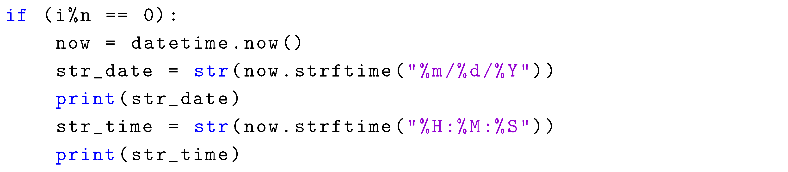
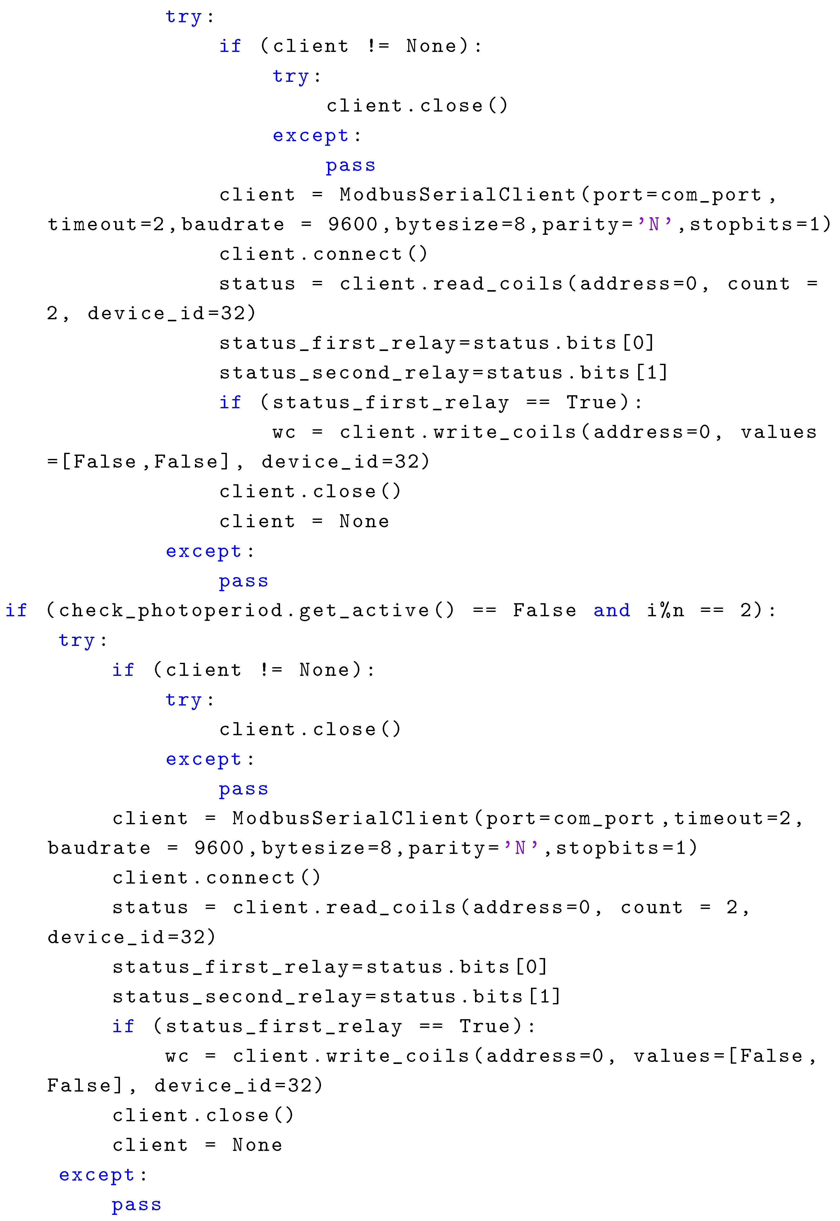
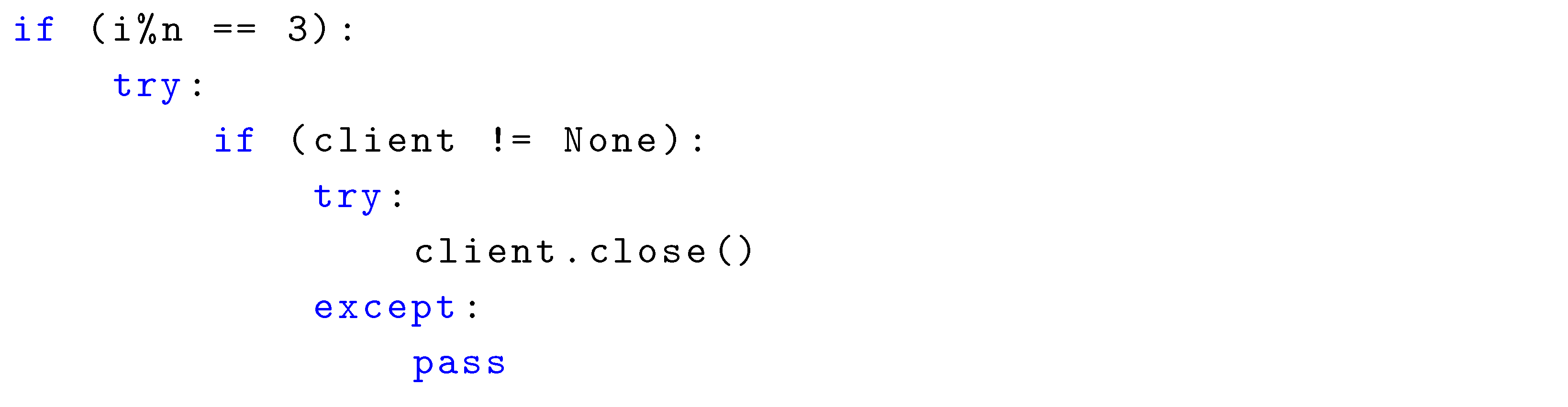
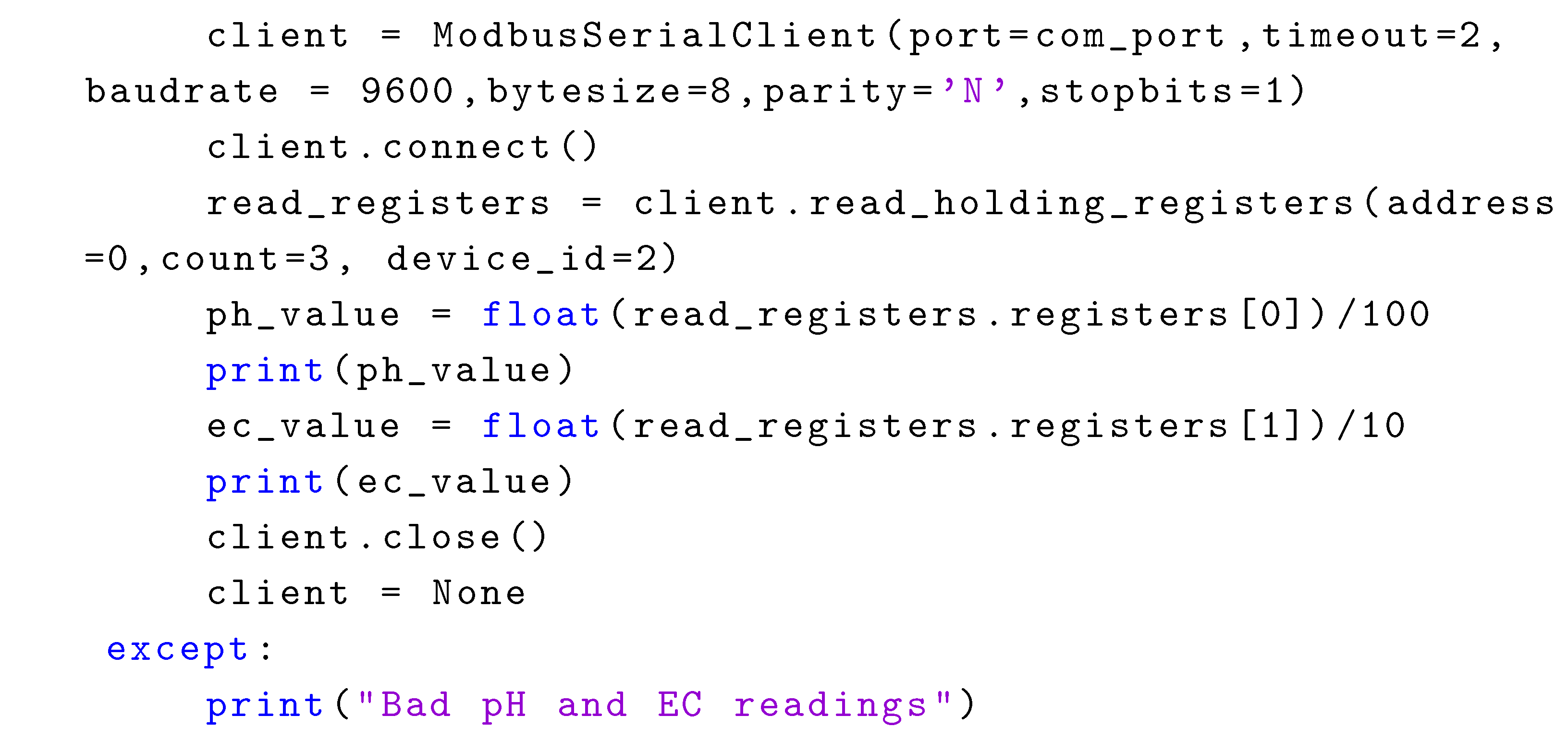
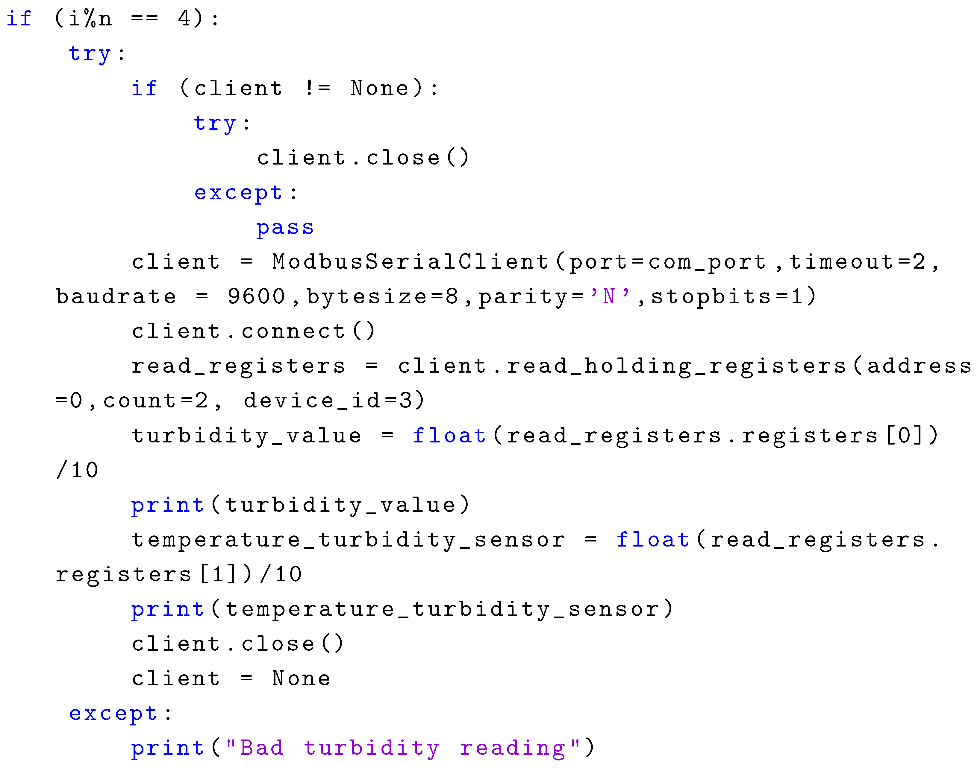
Appendix A includes the Python code snippets used in managing information in the Python application following the flow diagram sequence shown in Figure 2. However, it is essential to clarify that the app uses the object-oriented programming paradigm. Still, the Python code snippets shown in Appendix A are based on structured programming for simplicity. The Appendix A.1 shows the use of the datetime package to obtain the date and time from the PC operating system.
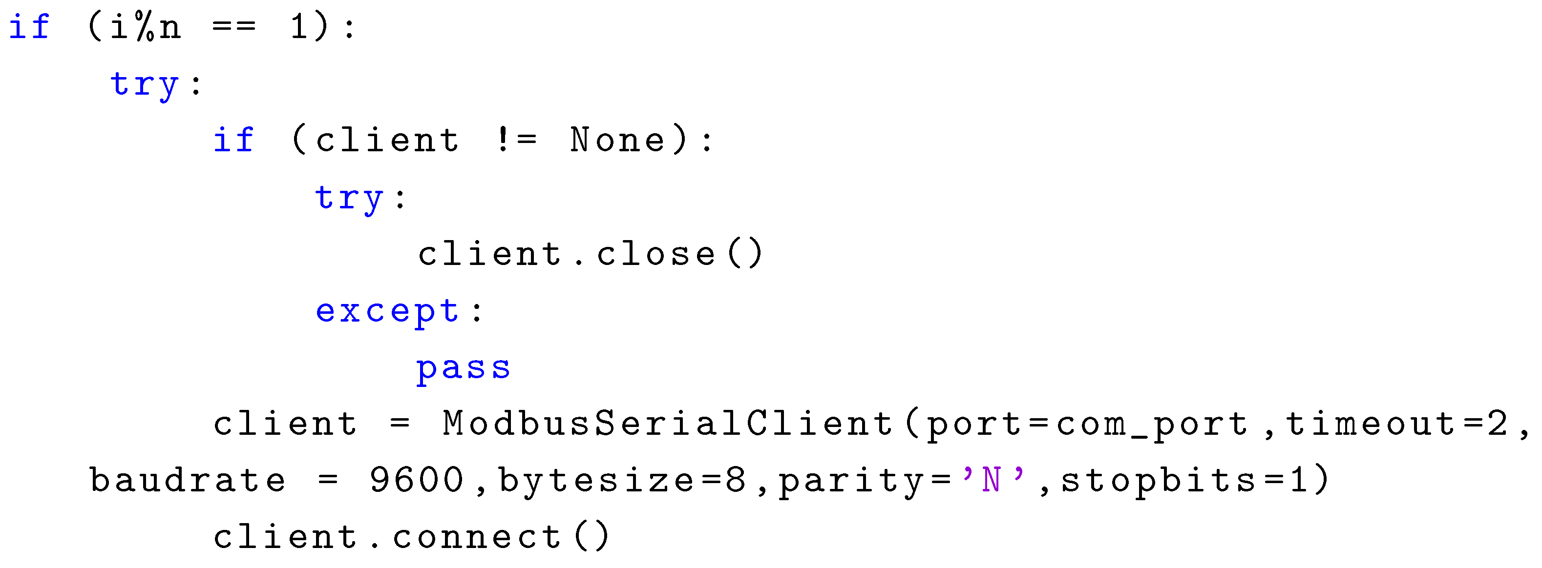
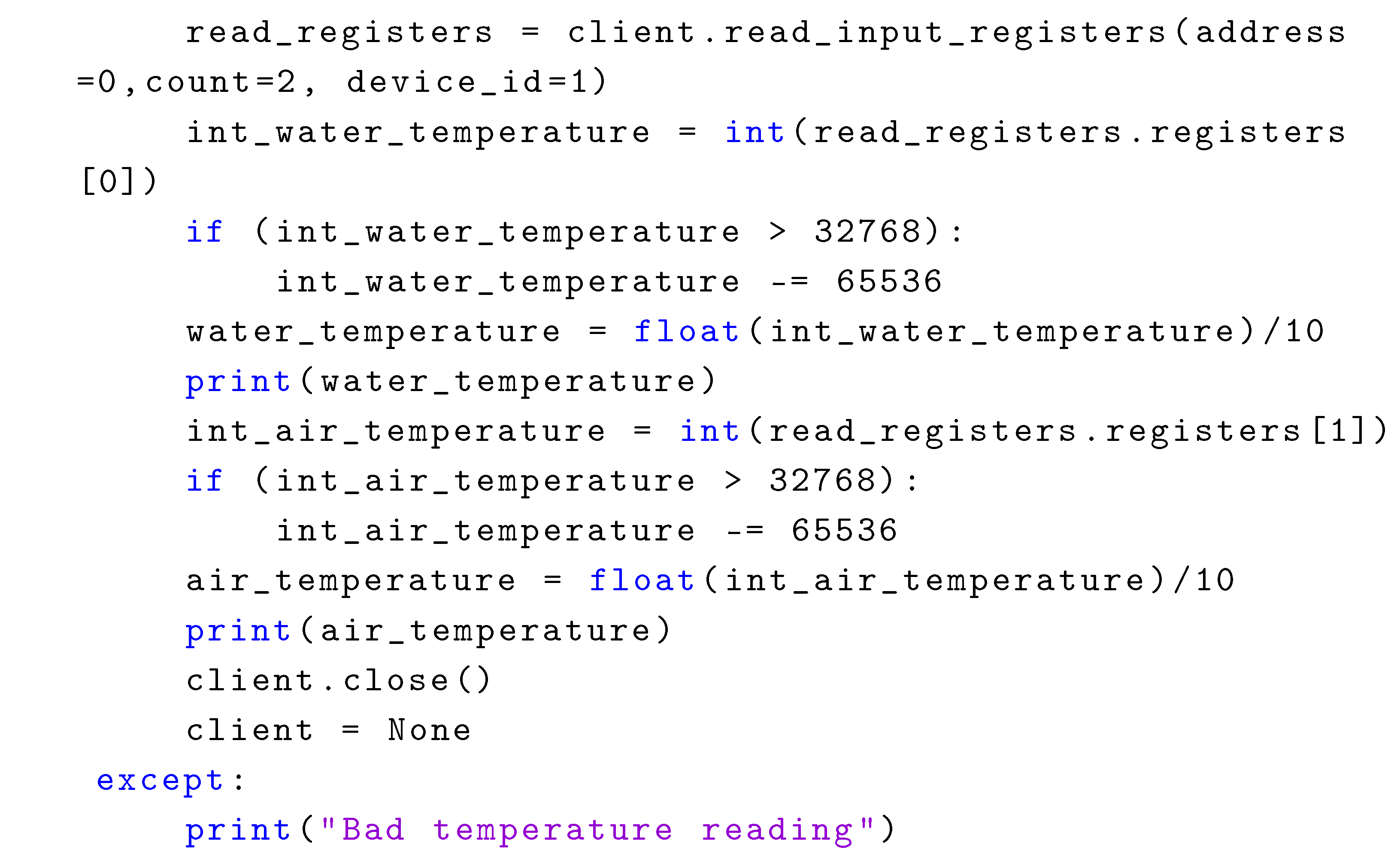
Appendix A.2 shows how to obtain the water and air temperatures. The code uses the ModbusSerialClient class from the PyModbus package to initialize communication with the USB-to-RS485 converter. The com_port variable of the client object corresponds to the serial port assigned to the converter by the operating system and is of type string. The temperatures are read with function 04 shown in Table 4, returning two registers of data type uint16. Any register with a value greater than 0x8000 requires a 0x10000 subtraction, which occurs when the temperature is negative. Dividing the values by 10 gives the final temperature. The parameters of the PyModbus methods are in decimal format. On the other hand, in the Windows operating system, it is advisable to open and close the ports every time a call is made to a server device as recommended by the MinimalModbus package documentation [60]; for that reason, in most of the Python code snippets presented in Appendix A, the client object is always created, and once a data read or write operation is performed, it is closed.
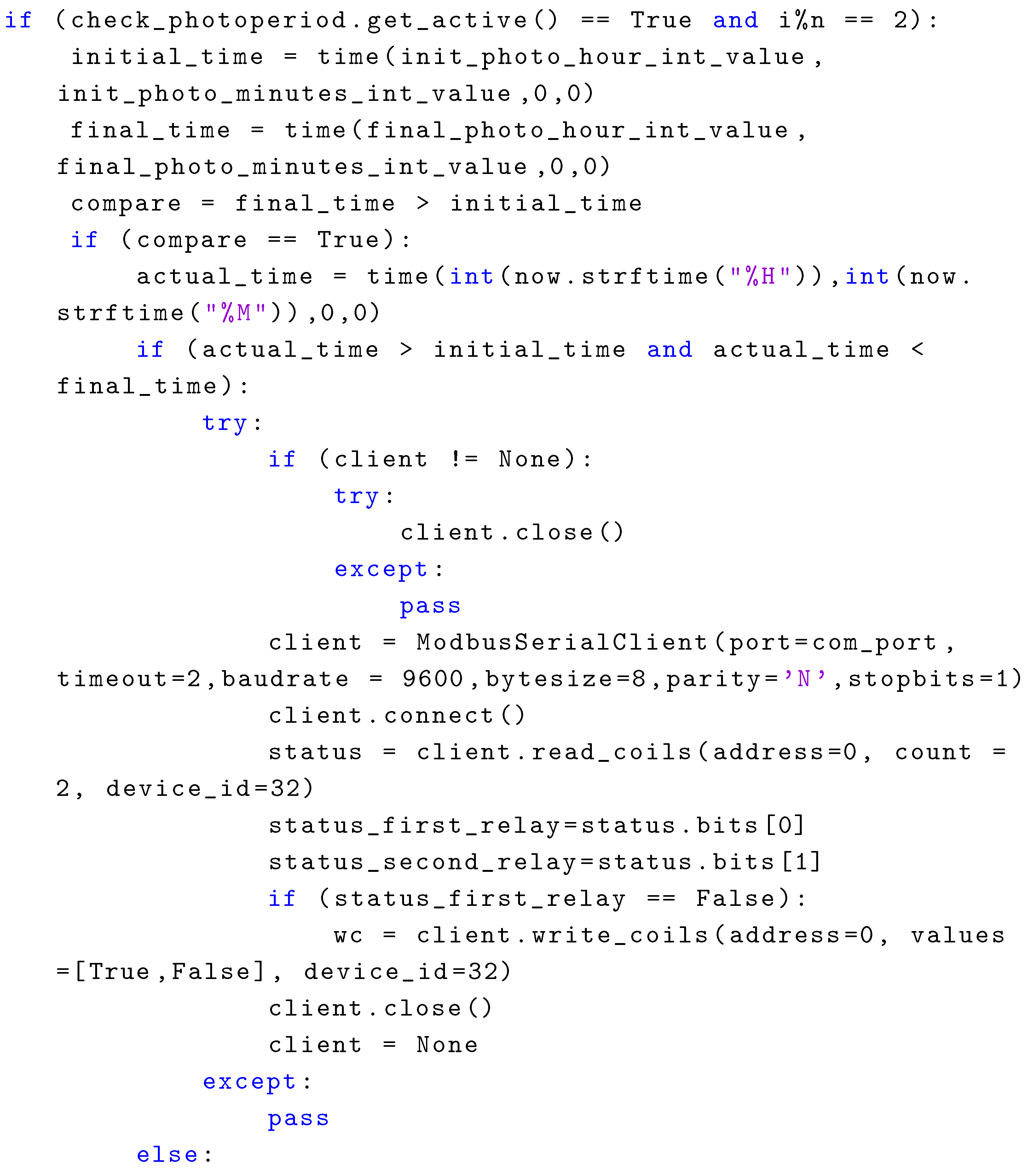
A check button in the main app window turns the photoperiod on or off. Appendix A.3 shows the Python code snippet for changing the state of the switch on the MA01-AACX2220 I/O device, which controls the illumination. The main window contains spin buttons for entering the hour and minute in 24 h format for the photoperiod’s start and end times. The now object in the code is the same as the one in Appendix A.1. If the time read from the computer’s operating system indicates that the light must turn on, with the aid of Modbus function 02, the first switch is closed. Modbus function 01 determines the status of the first switch (open or closed). A true boolean value indicates that the switch is closed; otherwise, it is open. The last part of the code verifies that the first switch is open when the photoperiod is disabled.
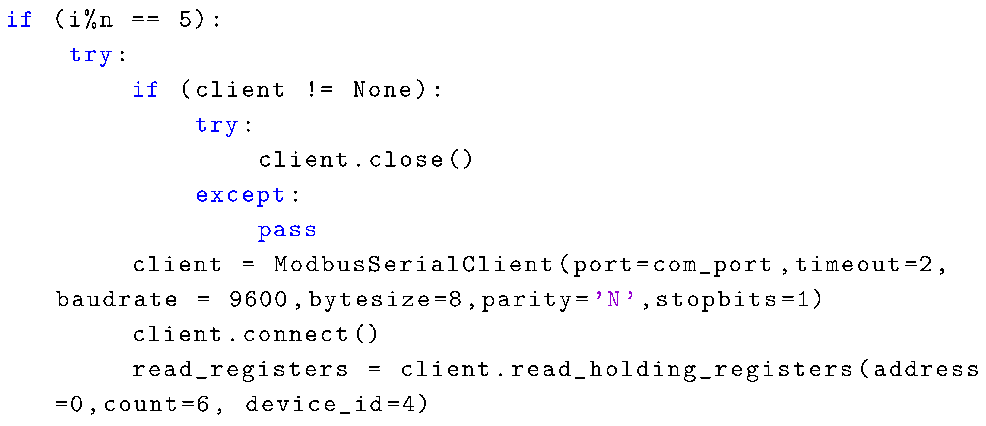
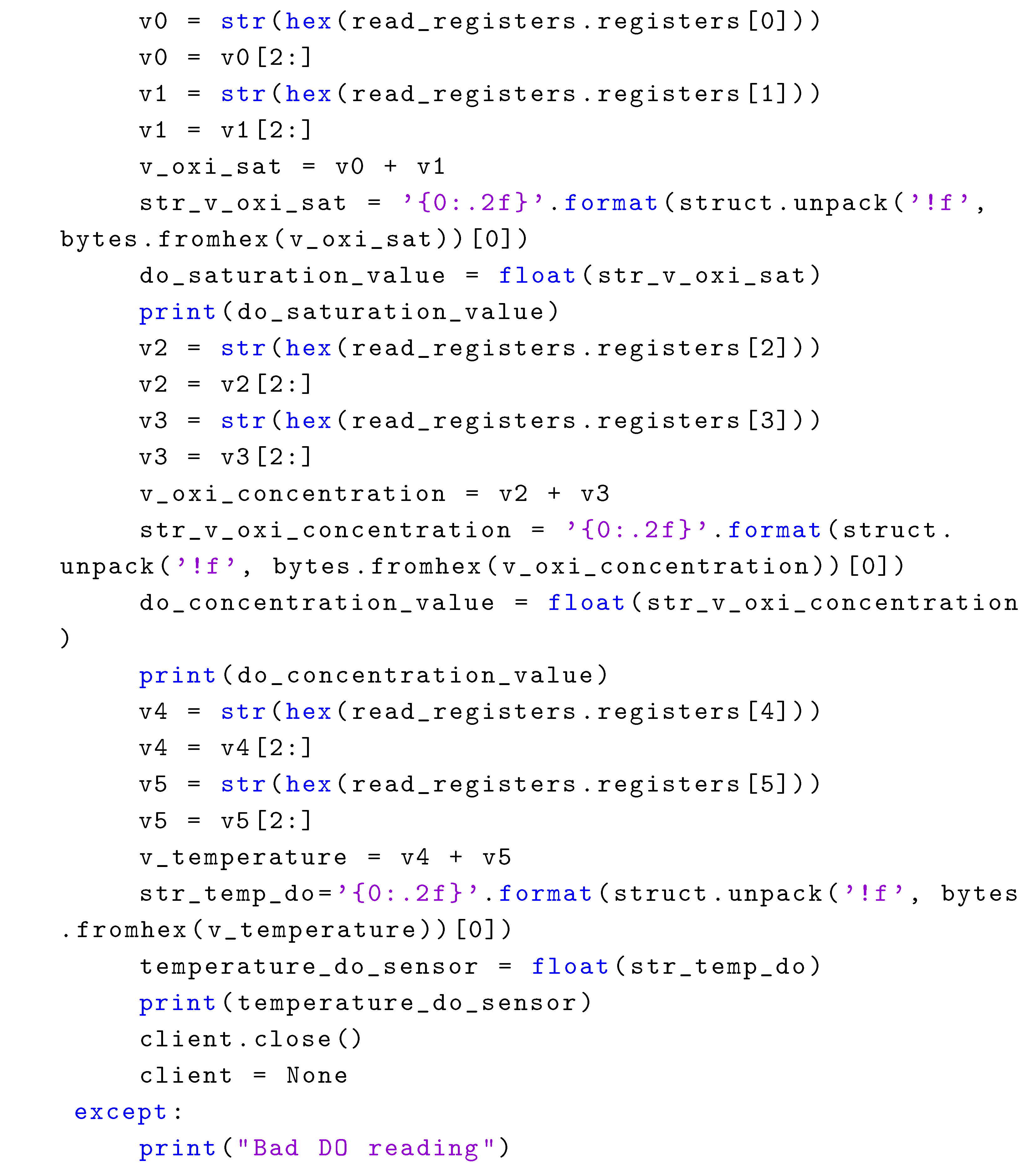
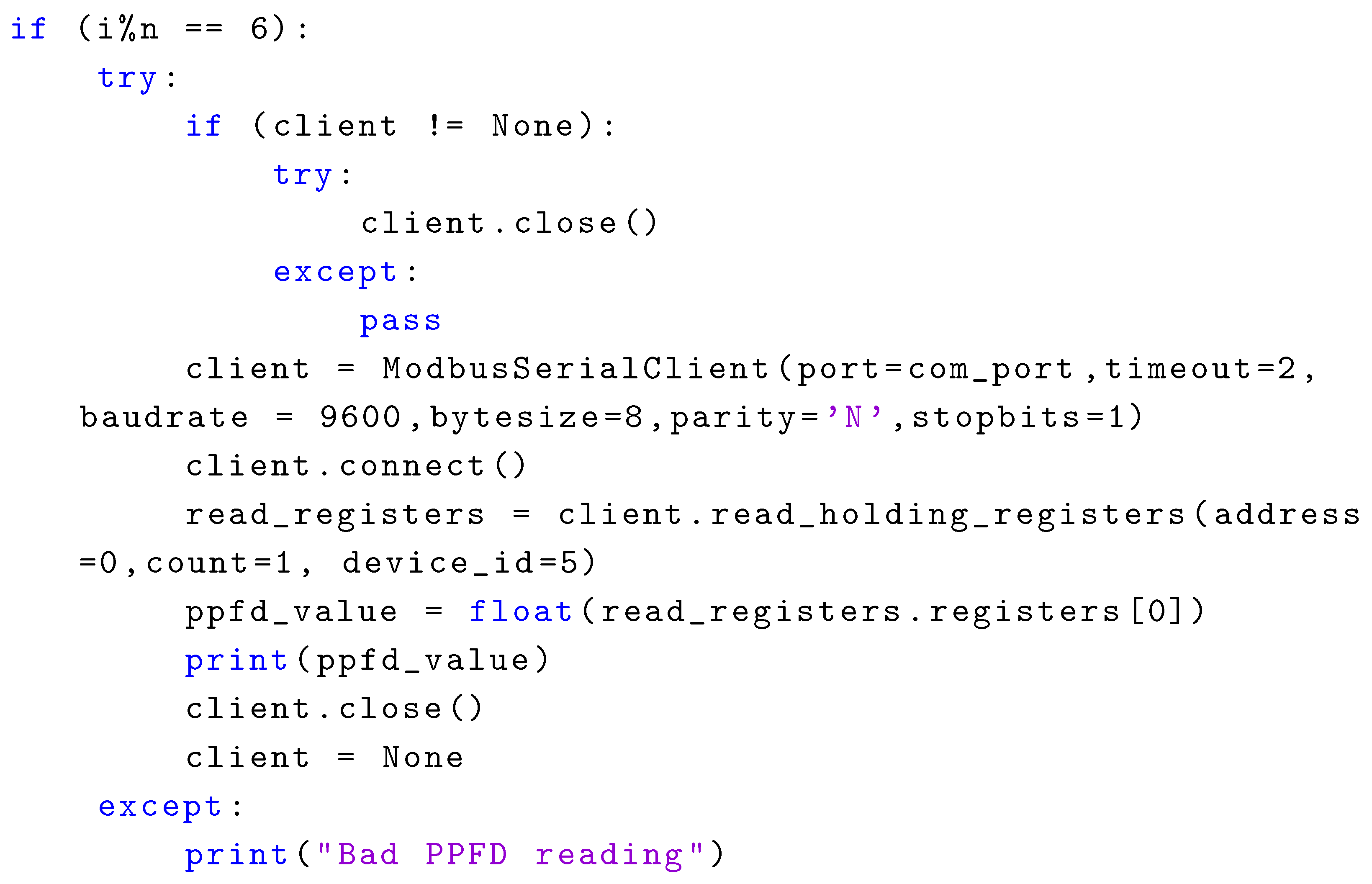
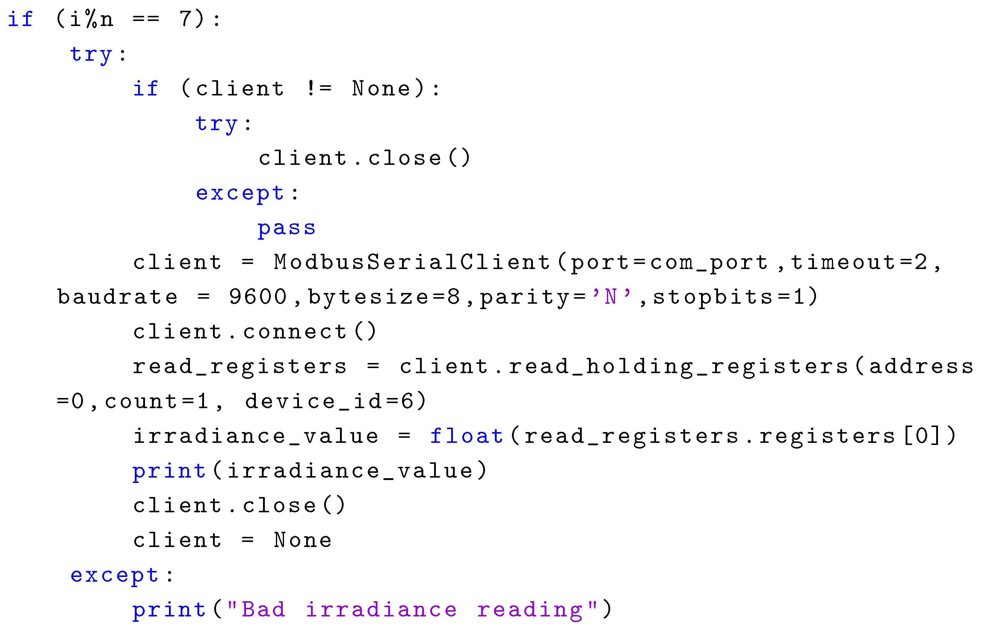
The Modbus function code 03 retrieves pH and EC sensor readings from a single Modbus module. Appendix A.4 shows the Python code snippet to obtain those measurements. The first register corresponds to the pH value, and the latter to the EC magnitude. Both registers required division: the first by 100 and the second by 10 to obtain the correct scale. Appendix A.5 shows the Python code snippet to read the turbidity. The sensor also measures the temperature. The DO sensor gives three measurements: dissolved oxygen saturation (%), dissolved oxygen concentration (mg/L), and temperature. Appendix A.6 shows a Python code snippet to perform the three readings with the DO sensor. Unlike the other sensors presented in this work, the register addresses are not integers; they are big-endian floats. The client’s request for the sensor consists of six registered addresses. Each of the three measurements requires concatenating the values of two register addresses in hexadecimal format. The two concatenated values are converted to their floating-point representation using the Python struct package. Appendix A.7 shows the Python code snippet for reading the PPFD, and Appendix A.8 exhibits the Python code snippet to obtain the value of irradiance.
The Python application is hosted on the GitHub repository https://github.com/JorgeFonsecaCampos/Python-program-for-reading-Modbus-RTU-sensors. (accessed on 12 June 2026).
2.7. Microalgae Strains and Culture Conditions
Biological systems present a complex dynamics. To mitigate the natural variability of their behavior requires experimental replication. Thus, we employed three Modbus systems to monitor the microalgae culture in three acrylic-walled bubble-column photobioreactors (PBRs) operated in batch mode. They had a capacity of 5 L, but the cultures operated at 3.5 L with continuous aeration at 0.14 vvm.
2.7.1. Microorganism
Chlorella vulgaris from the Microbial Culture Collection of Mexican Tecnológico de Estudios Superiores de Ecatepec (TESE) was the microalgae strain monitored with the Modbus platform proposed in this work. The microalgae were maintained on C-30 medium agar plates containing 5 g/L of KNO3, MgSO4 7H2O g/L, 1.25 g/L KH2PO4, 0.1 g/L K2HPO4, and 20 g of agar.
2.7.2. Inoculum Preparation
We grew the inoculum by placing 10% v/v of Chlorella vulgaris in the exponential growth phase in a 500 mL Erlenmeyer flask with a working volume of 350 mL for 5 days under continuous aeration, a 12L/12D photoperiod, and at room temperature.
2.7.3. Kinetics Experiments
The culture’s operating volume of 3.5 L initiated with 10% inoculum of C. vulgaris in the exponential growth phase. The cultures were incubated at 12L/12D and room temperature with continuous aeration at 0.14 vvm. Samples were collected every 24 h for several days to measure growth (mg/L). Kinetic experiments were carried out in triplicate.
2.8. Physical Implementation of the Proposed Platform
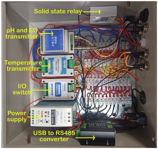
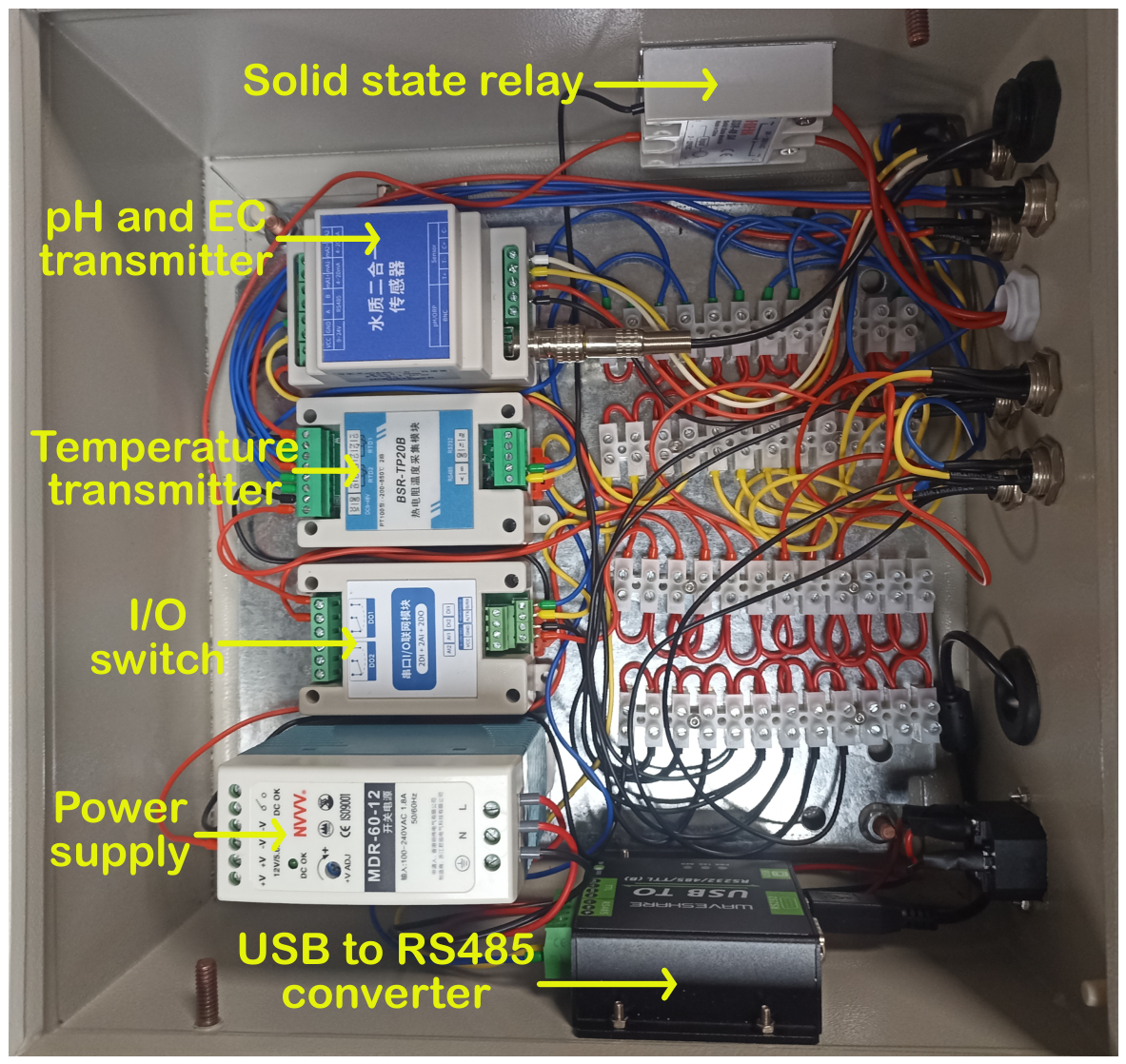
Figure 4 shows the enclosure box designed to protect certain elements of the proposed system from external environmental conditions. It included the power supply MDR 60-12 from the Taiwan Mean Well company (New Taipei City, Taiwan), rated to provide 12 VDC and 5 A, and the USB to RS-485 converter, the MA01-AACX2220 device, which controlled the solid state relay receiving DC signals to switch the AC line of the illumination, the temperature transmitter, and the pH and EC Modbus module. Also, several aviation connectors were mounted on the enclosure box wall to connect the remaining sensors.
Figure 4.
Enclosure box with the control and measurement modules.
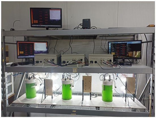
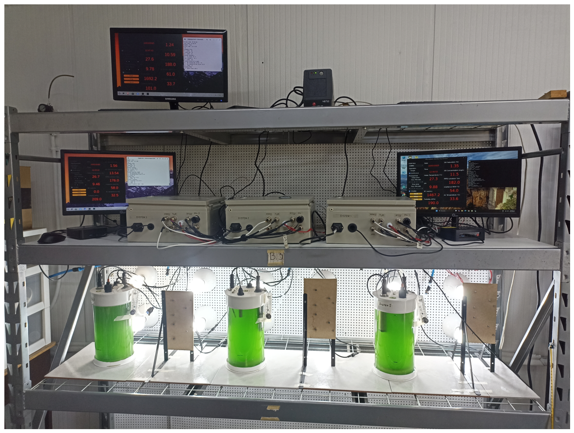
Figure 5 exhibits three photobioreactors with microalgae culture illuminated with white LED light bulbs. Also, it shows three cabinets, each dedicated to monitoring a PBR. The PPFD and the irradiance sensors were in front of the LED bulbs. The turbidity, DO, EC, and temperature sensors were inside the PBRs, in contact with the culture medium. Three mini PCs—two generic mini PCs with an Intel N5095 processor, 8 GB RAM, and a 256 GB SSD running Linux Zorin OS, and the other Mini PC, a Beelink model MINI S with an N95 processor, 8 GB RAM, and a 256 GB SSD running Windows—monitored and controlled the Modbus devices.
Figure 5.
Monitored and controlled photobioreactors.
3. Results and Discussions
In any data acquisition system, it is important to test its stability under non-aggressive conditions. Over 13.5 days, the Modbus sensors operated in aerated distilled water at 0.24 vvm to verify system response without interference from microorganisms that modify the temporal dynamics of some physicochemical variables; Section 3.1 presents the results with aerated water. Section 3.2 presents the time series acquired during the cultivation of C. vulgaris. Finally, Section 3.3 presents an additional experiment involving dissolved oxygen with the interruption of aeration in two separated daily periods of 6 h.
3.1. Time Series with Aerated Water
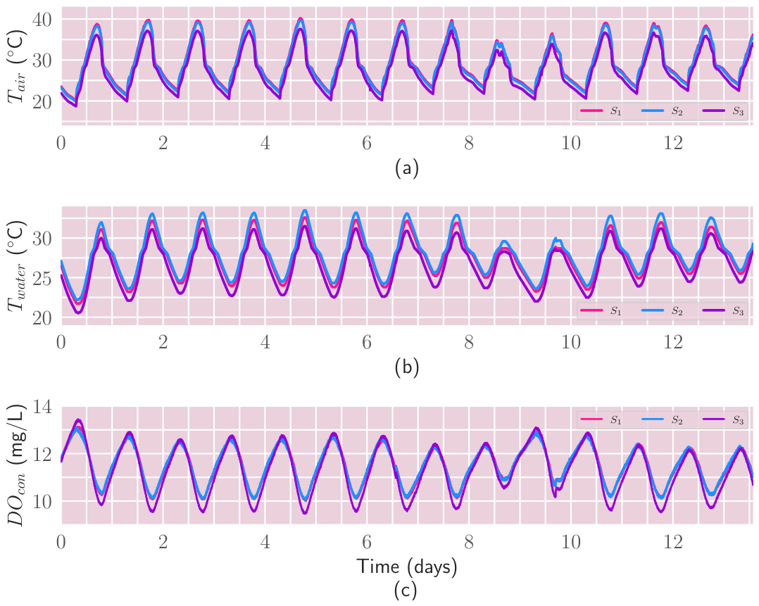
Microalgae cultures use CO2 as a carbon source [62], and the injected air in the PBR culture adds CO2 to the aquatic medium. Air bubbles also help homogenize the culture and prevent excessive self-shading by microalgae. Given the importance of aeration in microalgae cultivation, it is reasonable to evaluate the sensor response under these conditions. Initially, we set up three PBRs with distilled water for approximately 13.5 days in a laboratory with an air flow rate of 0.25 vvm. The experiment started on 25 February and lasted to 10 March 2026. During this time, the sensor system collected time-series data for air and water temperatures, pH, EC, DO, PPFD, irradiance, and turbidity. This experiment allowed the evaluation of sensors’ performance under conditions similar to those encountered during microalgae cultivation. Figure 6 shows the time series of temperatures measured with the CWT-BSR-TP20B and PT100 sensors, and the oxygen concentration acquired with the VMS-3002-LDO-N01-20 sensor in the three photobioreactors.
Figure 6.
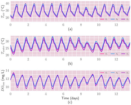
Variables exhibiting circadian oscillation: (a) Air temperature, (b) Water temperature measured with the PT100 sensor, and (c) Dissolved oxygen concentration. , , and correspond to the first, second, and third PBR, respectively.
Solar radiation is one of the variables that significantly modifies the weather. In particular, it has a notable influence on ambient temperature; the variation of solar flux on a surface throughout the day causes the temperature to exhibit a circadian oscillation, as shown in Figure 6a. The average air temperature was 29.3, 29.07, and 27.47 °C for PBRs , , and , respectively. The standard deviation was 5.26, 5.2, and 4.92 for PBRs , , and , respectively. The peak temperature reached magnitudes of up to 40.2, 39.6, and 37.6 °C for PBRs , , and , respectively. The ambient air had its minimum magnitudes of 20.2, 19.9, and 18.7 °C for PBRs , , and , respectively. In Mexico City, México, during the 13.5 days of the experiment, the average sunrise was at 6:53 a.m., and the average sunset was at 6:42 p.m., with a day length of 11 h and 48 min. On average, the minimum recorded air temperature was at 6:53 a.m. for the PBRs and , and at 6:56 a.m. for the PBR , implying that at sunrise, the solar radiation began to increase the laboratory temperature. At 3:53 p.m., 3:47 p.m., and 3:43 p.m., the Modbus sensor systems recorded the peak temperatures of the time series in PBRs , , and , respectively. Although solar radiation peaks at midday, the air temperature continued to rise until a few hours before sunset. Microalgae are not directly affected by weather temperature, but this variable modifies the temperature of the culture medium, which is why it is important to measure it.
The air surrounding the photobioreactors transfers heat to the culture medium, which in this experiment was distilled water. Water has a thermal conductivity approximately 20 to 25 times higher than air; this difference influences the magnitude observed of the time series for both variables. In fact, the water temperature is lower compared with the air temperature, as shown in Figure 6b, with average temperatures of 27.49, 28.06, and 26.5 °C for PBRs , , and , respectively. The standard deviations were 2.53, 2.67, and 2.64 °C for PBRs , , and , respectively. The highest peak temperatures reached by the PBRs were 32.6, 33.5, and 31.5 °C for PBRs , , and , respectively. The lowest recorded temperatures were 21.7, 22.2, and 20.5 °C for PBRs , , and , respectively. The PBR temperatures were within the range recommended in the literature [16]. The thermal conductivity of air and water also induces a lag between the temperature time series. Considering the peak values recorded, the maximum magnitude was at 5:55 p.m., 6:00 p.m., and 5:50 p.m. for PBRs , , and , respectively, implying a lag of approximately two hours with respect to the air temperature. Regarding the minimum temperatures recorded, the lag was smaller, since the average minimum values occurred at 7:31 a.m., 7:11 a.m., and 7:24 a.m. for PBRs , , and , respectively. Because the time series of water and air temperatures are out of phase, the Pearson correlation between the two time series across the three photobioreactors is not close to 1. Using the pearsonr function from the SciPy package of Python, the Pearson correlation obtained was 0.6235, 0.6540, and 0.6561 for PBRs , , and , respectively. The magnitudes of the correlation imply that not every time that the air temperature rose, the water temperature also rose, and vice versa.
Studies in Chlorella vulgaris cultivated in photobioreactors have shown that a high concentration of dissolved oxygen has adverse effects on biomass productivity [54]. During photosynthesis, microalgae consume CO2 and release O2, which can lead to excessive dissolved oxygen in the culture medium. Dissolved oxygen monitoring in distilled water helps identify the temporal evolution of this variable without microalgae cultivation. The dissolved oxygen concentration shown in Figure 6c had a mean of 11.50, 11.51, and 11.29 mg/L with a standard deviation of 0.79, 0.77, and 1 mg/L for PBRs , , and , respectively. Dissolved oxygen exhibited a circadian pattern with an average peak value of 12.63, 12.65, and 12.74 mg/L, and an average minimum value of 10.22, 10.22, and 9.70 mg/L for PBRs , , and , respectively. The average times at which the peak value occurred were 7:47, 7:11, and 7:55 a.m., and the minimum was at 6:30, 6:18, and 6:15 p.m. for PBRs , , and , respectively. These times have an inverse relationship with the water temperature, differing in their peaks and valleys by about a few minutes, since the water temperature is at its minimum when the dissolved oxygen concentration is at its maximum, and vice versa. Other authors have already reported an anticorrelation between these two variables [63,64]. The Pearson correlation using the pearsonr function from the Python SciPy package between the time series of water temperature and dissolved oxygen concentration was , , and for PBRs , , and , respectively. This is higher than the correlation obtained against air temperature , , and for PBRs , , and , respectively, as expected, because water retains oxygen.
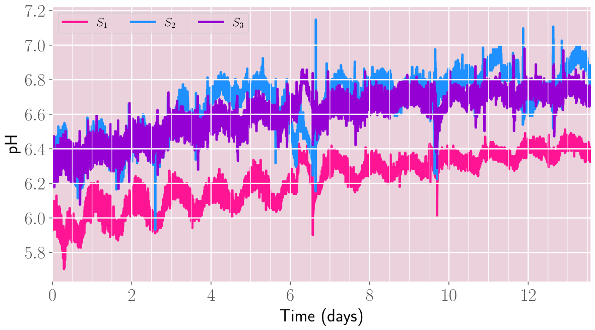
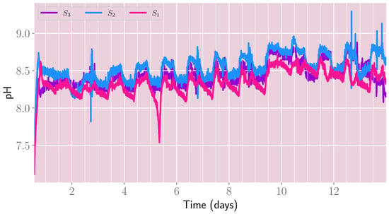
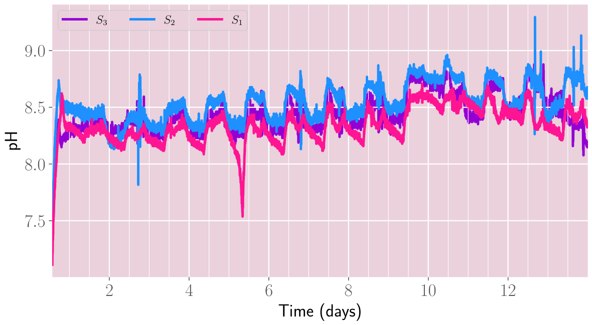
pH is one of the most critical variables in the monitoring of microalgae culture, because, due to microalgal photosynthesis, there is an induction of alkalization of the aquatic environment [65]. However, for aerated water, pH should remain almost constant, although it depends on temperature [9]. Figure 7 shows the time series of pH recorded for about 13.5 days, which had a mean of 6.21, 6.65, and 6.60, with a standard deviation of 0.147, 0.172, and 0.134 for PBRs , , and , respectively. We calibrated the three pH sensors using three standard pH solutions at 4.01, 7.01, and 10.01. The sensors showed a linear relationship with a correlation coefficient of 0.999. The calibration equations were , and , where , , and were the calibrated pH values and the magnitudes measured with the sensors for PBRs , , and , respectively.
Figure 7.
Time series of pH of aerated water. , , and correspond to the first, second, and third PBR, respectively.
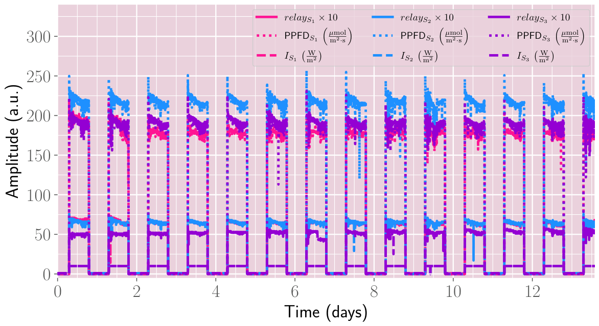
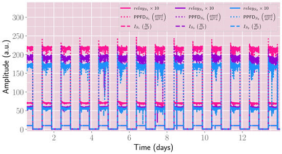
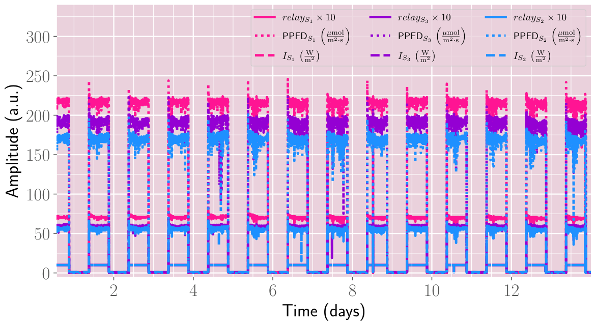
Figure 8 shows the variables related to light control and measurement. In Figure 8, , , and correspond to the activation of the relay of the module MA01-AACX2220 I/O device, for the first, second, and third PBRs, respectively. The activation signal recorded as a 1 was multiplied by 10 (solid lines). The photoperiod during the experiments consisted of illumination from 9:00 a.m. to 9:00 p.m., and darkness the rest of the day. White LED light bulbs used to illuminate the culture emitted almost photosynthetic radiation, with wavelengths between 400 and 700 nm. The average PPFD value (dotted lines) with the light activated was 180.06, 217.97, and 190.29 μmol/m2·s with the standard deviation of 7.20, 7.11, and 6.56 μmol/m2·s for PBRs , , and , respectively. The irradiance (dashed-dotted lines) under the same circumstance averaged 64.73, 65.39, and 52.26 W/m2 with a standard deviation of 2.3, 2.31, and 2.61 W/m2 for PBRs , , and , respectively. In general, the light was highly uniform.
Figure 8.
Variables related to PBRs illumination. , , and correspond to the first, second, and third PBR, respectively.
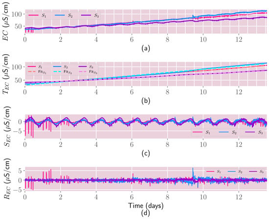
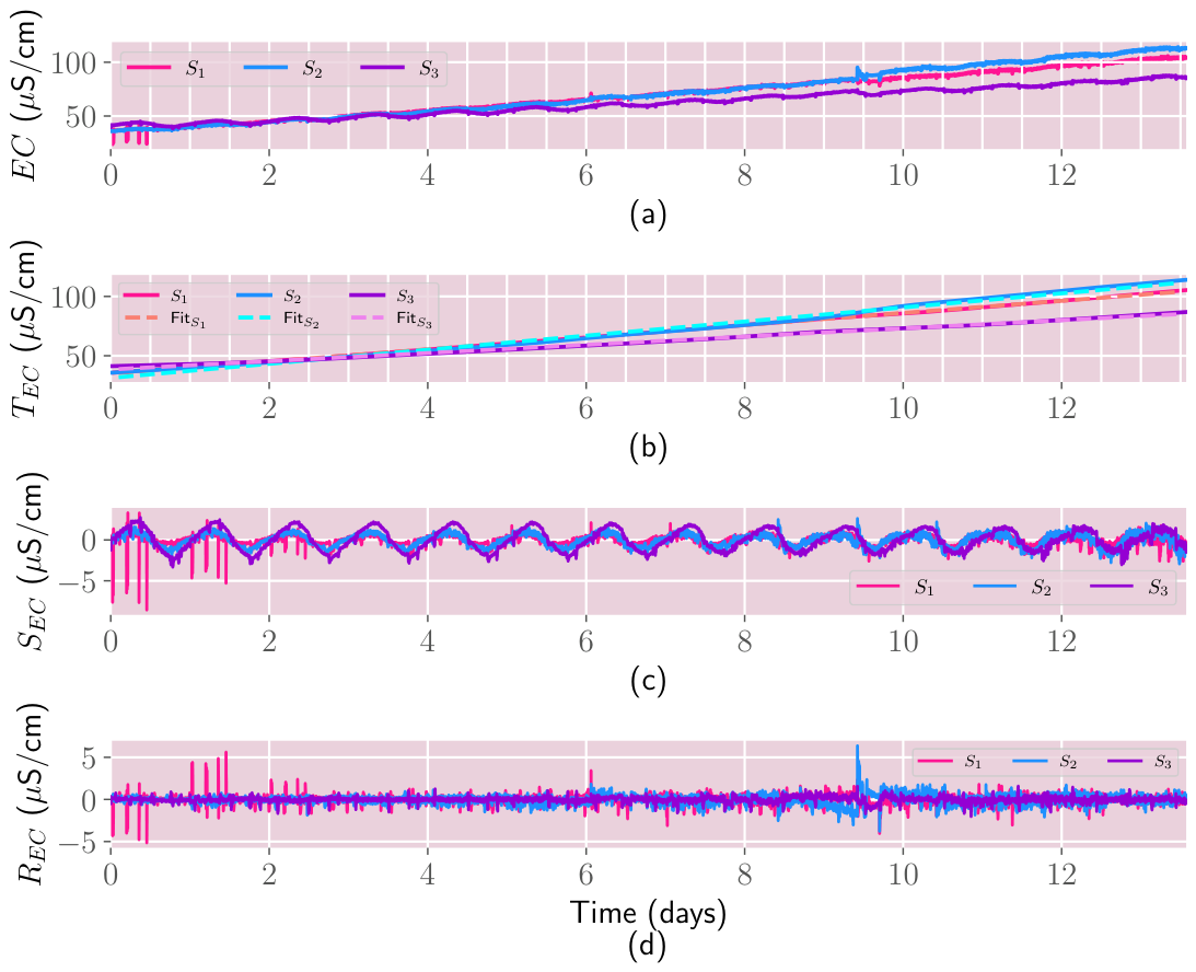
Culture media for microalgae usually have added metals in small quantities. Also, some microalgae strains require salts in their medium. Both elements tend to increase the electrical conductivity. During experiments measuring EC in aerated water, conductivity increased slowly, most likely due to dust particles introduced by the injected air. And during experiments with C. vulgaris, shown in the following subsection, the EC saturated because the medium’s electrical conductivity exceeded the sensor’s range. In distilled water, the conductivity grew linearly; therefore, we employed a widely employed tool in time series analysis, which is the decomposition with an additive model [66], given by
where is the original time series, is the trend, is the seasonality, and is the residual or random component. The Python package statsmodels in its version 0.14.4 includes the function season-trend decomposition using LOESS (STL) to fit an additive model to a time series. STL can calculate , , and for any time series. Figure 9 shows the recorded EC time series and its decomposition for the three PBRs.
Figure 9.
Additive model decomposition for EC during measurements in distilled water: (a) Original time series, (b) Trend, (c) Seasonality, and (d) Residuals. , , and correspond to the first, second, and third PBR, respectively.
Figure 9a shows the original EC time series. Figure 9b shows The EC trend which is linear following the fitted equations , , and μS/cm, with a correlation coefficient of 0.9998, 0.995, and 0.998 for PBRs , , and , respectively. In the above equations, t is the time in decimal days. Figure 9c shows that there is a quite small seasonality component with an average magnitude of 0.001, 0.016, 0.037, with a standard deviation of 0.613, 0.770, and 1.274 for PBRs , , and . has a magnitude much smaller than the that predominates in the EC time series. Finally, the residuals shown in Figure 9d had an average of , , and with a standard deviation of , 0.520, and 0.308 μS/cm for PBRs , , and , which represents mostly white noise.
The water turbidity sensor exhibited significant noise and outliers across the three PBRs; therefore, we omitted the time series. The noise might have come from the air bubbles, and to mitigate it, a static water sample is required.
A few key points emerge from summarizing the time series results for aerated water. The proposed platform registered the variables without losing data, a crucial aspect. The variables measured in the three PBRs were, in most cases, very similar, ensuring that the PBRs were under similar physical conditions. The time series for most sensors has almost no outliers. The variability of most sensors in most practical applications may be negligible.
3.2. Time Series During the C. vulgaris Culture
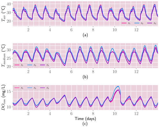
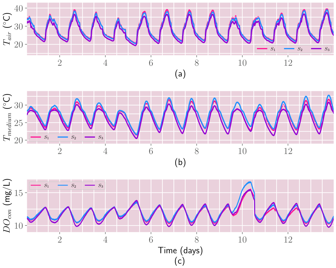
Figure 10 shows the time series related to temperature and dissolved oxygen during approximately 13.5 days of the cultivation of Chlorella vulgaris. The experiment started on 13 March and finished on 26 March 2026. These time series showed mostly a circadian cycle driven by the natural solar cycle, except for , which exhibited an anomaly for approximately 14 h, as explained below. The average air temperature denoted as and shown in Figure 10a was 28.99, 28.6, 27.16 °C, and the standard deviation was 5.2, 5.07, and 4.81 °C for PBRs , , and , respectively. Due to the fact that these experiments followed the measurements with distilled water, the average time at which the air temperature reached its maximum is quite similar to the previous experiments. For example, the average maximum value was at 3:44, 3:43, and 3:37 p.m., meanwhile the minimum average value was at 7:13, 7:15, and 7:10 a.m., for PBRs , , and , respectively.
Figure 10.
Variables exhibiting circadian oscillation during cultivation of Chlorella vulgaris: (a) Air temperature, (b) Microalgae medium measured with the PT100 sensor, and (c) Dissolved oxygen concentration. , , and correspond to the first, second, and third PBR, respectively.
Figure 10b shows the temperature of the microalgae medium denoted as . The average temperature was 26.93, 27.41, and 26.01 °C, with the standard deviation of 2.401, 2.56, and 2.528 °C for PBRs , , and , respectively. The average maximum temperature was 30.09, 30.92, and 29.2 °C, and the average time of the peak value was 5:46, 5:49, and 5:41 p.m. for PBRs , , and , respectively. The average minimum temperature of the culture medium was 23.16, 23.47, 22.11 °C reached on average at 8:13, 8:29, and 8:29 a.m. for PBRs , , and , respectively. A comparison between the temperature recorded in distilled water presented in the previous subsection and that in this experiment shows that the weather conditions were quite similar, with an average difference of roughly 0.5 °C and peak values occurring at almost the same time, contrary to the minimum temperature, which in these experiments occurred an hour later.
Real-time monitoring is a valuable tool for identifying anomalies in the cultivation conditions. During part of the 9th and the 10th day, the compressor supplying air to the PBRs went offline due to a power outage. During this time, dissolved oxygen concentrations increased in the three PBRs, reaching levels above the average recorded on other days. Also, the lack of aeration altered the anticorrelation between and observed in these experiments and in those with aerated water, thereby influencing pH. Figure 10c shows the dissolved oxygen concentration during the microalgae cultivation. The average was 11.84, 12.02, 11.75 mg/L with the standard deviation of 1, 1.18, and 1.2 mg/L for PBRs , , and , respectively. The average peak value was 13.12, 13.35, and 13.35 mg/L while the average minimum value was 10.62, 10.73, 10.26 mg/L for PBRs , , and , respectively. In general, was higher at approximately mg/L than in experiments with distilled water. However, this increase may partly be due to the lower temperatures recorded during the microalgae experiments. The temporal evolution of with microalgae is somewhat unexpected, because these microorganisms are photosynthetic and, under illumination, produce oxygen. However, the time series does not correlate with light application; it is related to water temperature, at least when the culture receives pumped air. The Pearson correlation obtained with pearsonr function from the SciPy package of Python for the water temperature and was not as high as the one obtained with distilled water, being , , and for PBRs , , and , respectively. However, by filtering the time series, omitting the time where the aeration went off, the calculated Pearson correlation was , , and for PBRs , , and , respectively. The latter value is similar to the results obtained with distilled water. Further experiments involving dissolved oxygen are presented at the end of this section.
Figure 11 shows the PPFD, the irradiance, and the activation of the illumination during microalgae cultivation. The photoperiod was 12:12, and light was active from 9:00 a.m. to 9:00 p.m. The average PPFD was 216.34, 170.7, and 191.01 μmol/m2·s, with standard deviations of 5.173, 6.358, and 6.892 μmol/m2·s for the PBRs , , and , respectively. The average irradiance was 70.64, 56.05, and 59.05 W/m2 with the standard deviation of 1.601, 2.122 and 1.926 W/m2 for the PBRs , , and , respectively.
Figure 11.
Variables related to PBRs illumination during cultivation of Chlorella vulgaris. , , and correspond to the first, second, and third PBR, respectively.
Figure 12 shows the pH temporal evolution during the cultivation of Chlorella vulgaris. It clearly shows that the pH grew drastically by approximately 1.3 units during the first few hours after culture inoculation. The medium has a higher pH than distilled water, and most commercial microalgae tend to grow in an alkaline medium. The time series of pH exhibit a pattern that relates to illumination because the inorganic carbon species in algae culture depend on the removal of CO2 and the bicarbonate uptake during microalgae photosynthesis; usually, pH increases during the period of illumination and decreases during exposure to darkness due to respiratory CO2 release [67]. The average pH was 8.34, 8.53, and 8.43, with standard deviations of 0.153, 0.17, and 0.159 for the PBRs , , and , respectively. For the above reason, under illumination, pH was slightly higher, averaging 8.39, 8.62, and 8.50 for the PBRs , , and , respectively, compared with the pH in darkness, which averaged 8.29, 8.44, and 8.38 for the PBRs , , and , respectively. The pH magnitude was influenced by the absence of aeration when the compressor went offline during part of the 9th and the 10th day; it recovered its dynamics with aeration.
Figure 12.
Time series of pH during cultivation of Chlorella vulgaris. , , and correspond to the first, second, and third PBR, respectively.
During experiments with Chlorella vulgaris, the culture medium exceeded the operating range of the electric conductivity sensor. Also, the turbidity sensor did not work properly under aeration. Therefore, we omitted both time series in this subsection.
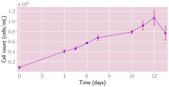
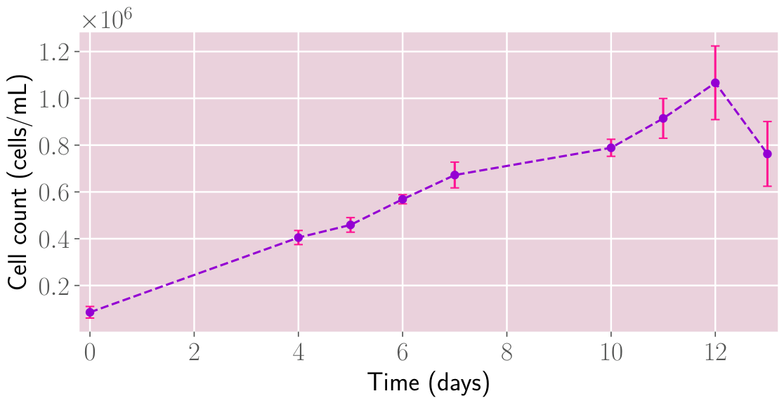
pH and dissolved oxygen are physicochemical variables related to the biomass quantity. Therefore, we collected samples of the microalgae culture over several days to estimate cell growth. We use an improved Neubauer hemocytometer (Proper Manufacturing Co., Inc., Long Island City, NY, USA) to perform this technique. Figure 13 shows the average cell count for the three PBRs. The C. vulgaris reached a stationary growth rate at 12 days; the plots show a clear increase in biomass during the cultivation period.
Figure 13.
Average cell count of Chlorella vulgaris for the three PBRs.
3.3. Additional Measurements of Dissolved Oxygen
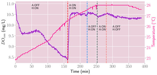
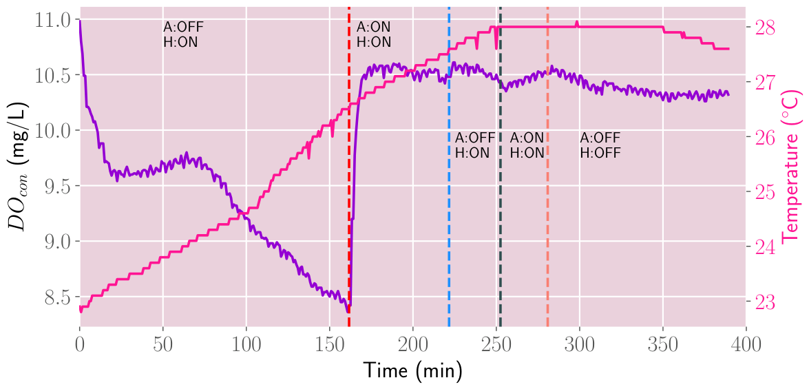
We decided to perform additional measurements of to phenomenologically describe the dynamics observed in the time series presented in the previous subsections. Figure 14 shows the measurement of (violet line) and temperature (pink line) of a PBR filled with water. During the first 161.6 min, the water temperature increased because the PBR was on a heating plate. Figure 14 shows that in this period of time, decreased due to the increase in temperature. The application of aeration from 161.6 to 221.6 min increased rapidly, reaching saturation as expected and stabilizing at approximately 10.5 mg/L. We turned off aeration from 221.6 to 252.5 min, but remained almost constant. The new application of aeration from 252.5 to 280.83 min did not significantly increase , which remained slightly below 10.5 mg/L. From 280.83 to 390 min, the heating element and aeration were off. The decrease in was very slow due to a loss of temperature and a lack of aeration. In conclusion, in water, the variable that influences the the most is the temperature, and of course, the initial quantity of air that has already dissolved in water.
Figure 14.
Time series of dissolved oxygen concentration in distilled water with controlled temperature and different conditions of aeration. In this figure, A means aeration, and H means heating. Also, the violet line corresponds to the dissolved oxygen concentration and the pink line to the water temperature, and the vertical lines indicate different time events.
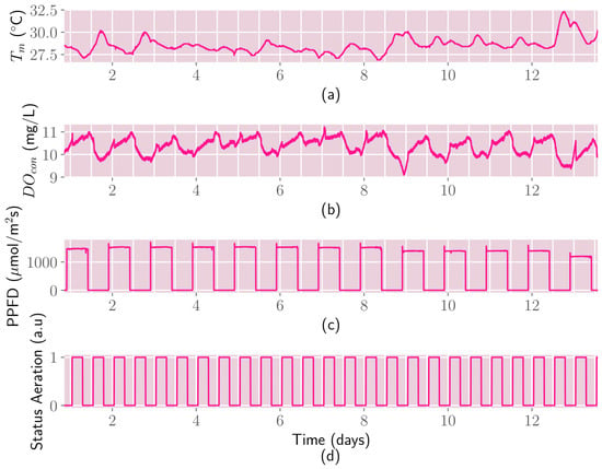
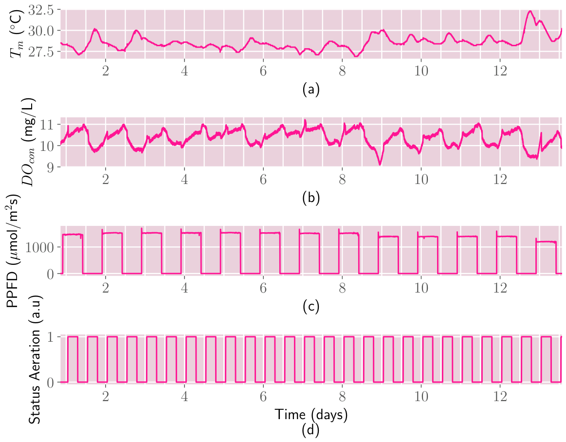
A recent report explained three strategies for mitigating excessive concentrations of dissolved oxygen in cultures of the microalgae strains Monoraphidium minutum 26B-AM and Scenedesmus obliquus UTEX393 [68]. The first involved increasing the concentration of sodium bicarbonate in the culture medium; the second, adding sodium sulfite to the microalgae; and the third, sparging the culture with air for 12 h a day. The latter strategy looked the most promising of the three, because it significantly reduced the dissolved oxygen and increased the biomass productivity of S. obliquus UTEX393 by 36%. The above results could explain to some extent the different dynamics exhibited by the dissolved oxygen concentration in the time series during the 9th and the 10th day shown in Figure 10c. However, we decided to run another experiment with C. vulgaris to investigate the anomaly in the time series. The experiment consisted of aerating a photobioreactor with the microalgae culture for 12 h a day in two 6 h periods: one from 1:00 h to 7:00 h and the other from 13:00 to 19:00 h, unlike the rest of the experiments, which used continuous aeration without interruption. This experiment included illuminating the PBR for 12 h, from 22:00 h to 10:00 h, and measuring the culture medium temperature, , and PPFD. Figure 15 shows the time series of the above variables and a unit step function representing the application of aeration. The experiments lasted 12.7 days, starting on 14 April and ending on 29 April 2026. A comparison of Figure 15a with Figure 15b shows that the high anticorrelation between the medium temperature and exhibited in previous experiments and shown in Figure 6 and Figure 10 diminished. In fact, the Pearson correlation between the two time series was . In this experiment, the application of light without aeration increased due to the liberation of O2 by photosynthesis. The application of aeration during illumination on some days reduced almost immediately the level of by increasing the kinetic energy of the medium, physically removing the dissolved oxygen, but on other days increased the as happened with water shown in Figure 14. It means that if the medium has not reached saturation, aeration could increase . Otherwise, when the level of the dissolved oxygen in the medium is higher than the saturated level, the aeration removes the excess of .
Figure 15.
Time series of a C. vulgaris culture with the interruption of aeration: (a) medium culture temperature, (b) , (c) PPFD, and (d) unit step function representing the application of aeration.
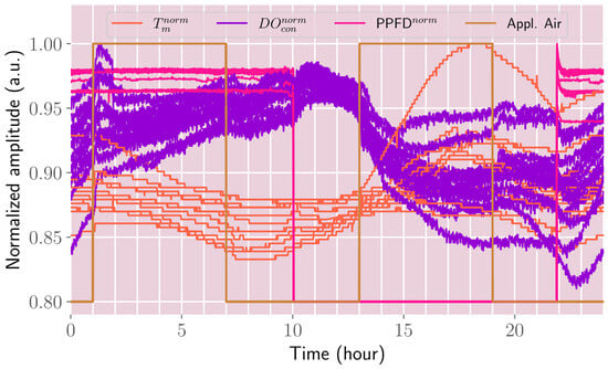
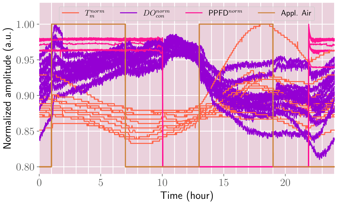
A circadian plot helps to have better insight into the features of the time series presented in Figure 15. Figure 16 shows such a plot after the normalization of the time series. (orange solid line) exhibits the typical circadian patterns having a minimum amplitude at ∼8:30 a.m., and its daily peak at ∼6:00 p.m. (violet solid line) clearly does not anticorrelate with as in the previous measurements under continuous aeration. The application of illumination without aeration at 10:00 p.m. produces a clear increase in the due to photosynthesis continuing with this trend up to 1:00 a.m., coinciding with the application of aeration, which modified the magnitude of sometimes reducing it, other times increasing it, depending of the initial magnitude of , whether it is amplitude was below or above saturation. Minutes after 1:00 a.m., with air and light applied simultaneously, increased, but at a lower rate than previously. At 7:00 a.m., without aeration but with light applied, dissolved oxygen increased, though at a further reduced rate. At 10:00 a.m., anticorrelated with temperature. At 1:00 p.m., aeration reduced the magnitude of . From 7:00 p.m. to 10:00 p.m., remained almost constant even though the temperature started to decrease. To summarize this experiment, it is clear that photosynthesis produces O2 that escapes from the culture with aeration. Also, the level of depends on illumination, aeration, temperature, and the quantity of biomass.
Figure 16.
Circadian temporal evolution of variables during the interruption of aeration. stands for normalized medium temperature, is the normalized dissolved oxygen concentration, is the normalized PPFD, and Appl. Air corresponds to the application of aeration.
4. Conclusions
This work presented the technical details of developing a Python-based Modbus sensor platform for monitoring photobioreactors containing microalgae cultures. Python is free and one of the most popular programming languages, with an extensive ecosystem of libraries that run on various operating systems. The Modbus protocol and Python are open, royalty-free ecosystems, and sensors based on this protocol are usually low-cost. Also, the system with customization can meet other needs. We also demonstrated a unique node-controlled Modbus sensor from different suppliers.
The application of the monitoring platform to microalgae cultures and aerated photobioreactors, in triplicate, showed that real-time monitoring enables the observation of both subtle and drastic changes in the culture’s physicochemical conditions, providing a valuable tool for improving cultivation practices. The platform recorded time series in three sets of experiments without loss of information and with a low rate of outliers.
Under aeration of the PBRs, the time series of and water or microalgae culture medium temperature exhibits a high anticorrelation ∼. Despite that, photosynthesis produces oxygen, and an increase in should be expected. However, aeration increases kinetic energy and, as a consequence, limits the dissolved oxygen that the medium can maintain. Experiments with aeration interruption showed that increased with photosynthetic activity, significantly reducing the anticorrelation between dissolved oxygen and medium temperature to . The above experiment showed that the level of depends on illumination, aeration, temperature, and biomass quantity. The temperature time series oscillated with the sun’s natural light-dark cycle. Under illumination, pH time series of the culture of C. vulgaris exhibited a higher average pH than without illumination, showing that during photosynthesis, CO2 is the inorganic carbon source for this process. The turbidity sensor readings in aerated water showed excessive noise; this sensor is not suitable for measurements under the conditions used in the experiments. The EC sensor’s operating range was insufficient for microalgae cultures, as the salts and trace metals required for their cultivation exceeded the sensor’s limits.
Studies of microalgae culture monitoring, as presented here, can help improve cultivation practices. These microorganisms are important because they can be the basis for third-generation renewable biofuels that can reduce CO2 emissions, avoid conflicts between food and fuel production, and achieve exceptional yields and efficiency.
Modbus RTU is slow for applications that require shorter sampling times; one option is to use sensors with Modbus TCP, which offer a faster data transfer rate.
Author Contributions
Conceptualization, J.F.-C. and L.C.F.L.; Methodology, J.F.-C., L.C.F.L., J.A.M.-P. and A.R.D.-B.; Software, J.F.-C., L.C.F.L., I.R.-R. and J.A.M.-M.; Sensor network, I.R.-R., J.A.M.-M., J.L.M.-M. and R.A.-L.; Investigation, J.L.M.-M. and R.A.-L.; Data analysis I.R.-R., J.A.M.-M., J.L.M.-M. and R.A.-L.; Experiments, J.F.-C., L.C.F.L., A.R.D.-B., J.A.M.-P. and R.A.-L.; Writing—original draft preparation J.F.-C., L.C.F.L. and A.R.D.-B.; Funding acquisition, J.F.-C., L.C.F.L. and A.R.D.-B. All authors have read and agreed to the published version of the manuscript.
Funding
This work was partially funded by the Secretaría de Investigación y Posgrado del Instituto Politécnico Nacional (SIP-IPN) through the grants IND-2026-0451 and MULTI-2026-0049-M4, and the Secretaría de Educación, Ciencia, Tecnología e Innovación de Ciudad de México (SECTEI-CDMX) through the grant 4244c24.
Institutional Review Board Statement
Not applicable.
Informed Consent Statement
Not applicable.
Data Availability Statement
The original contributions presented in this study are included in the article. Further inquiries can be directed to the corresponding authors.
Acknowledgments
The authors thank Secretaría de Investigación y Posgrado del Instituto Politécnico Nacional (SIP-IPN) and Comisión de Operación y Fomento de Actividades Académicas (COFAA-IPN) for the aid provided to perform this work. Jorge Fonseca-Campos would like to thank to Centro de Investigación y de Estudios Avanzados (CINVESTAV), Departamento de Biotecnología y Bioingeniería, for the aid provided to perform this work.
Conflicts of Interest
The authors declare no conflicts interest.
Abbreviations
The following abbreviations are used in this manuscript:
| ASCII | American standard code for information interchange |
| CRC | Cyclic redundancy check |
| CSV | Comma separated value |
| DO | Dissolved oxygen |
| EC | Electrical conductivity |
| FIR | Finite impulse response filter |
| GUI | Graphical user interface |
| I2C | Inter-integrated circuit |
| LED | Light emitting diode |
| LT | Line termination |
| NASA | National Aeronautics and Space Administration |
| NTU | Nephelometric turbidity units |
| PAR | Photosynthetic active radiation |
| PBR | Photobioreactor |
| PC | Personal computer |
| PLC | Programmable logic controller |
| PPFD | Photosynthetic photon flux density |
| PVC | Polyvinyl chloride |
| RTD | Resistance temperature detector |
| RTU | Remote terminal unit |
| SPI | Serial peripheral interface |
| TCP/IP | Transmission control protocol/internet protocol |
| TTL | Transistor-transistor logic |
| UART | Universal asynchronous receiver/transmitter |
| USB | Universal serial bus |
Appendix A
Appendix A.1. Code Snippet for Manipulating Dates and Times
Appendix A.2. Code Snippet for Obtaining the Temperature
Appendix A.3. Code Snippet for Enabling the Photoperiod
Appendix A.4. Code Snippet for Reading the pH and EC Sensors
Appendix A.5. Code Snippet for Obtaining the Turbidity
Appendix A.6. Code Snippet for Reading the DO Sensor
Appendix A.7. Code Snippet for Reading the PPFD Sensor
Appendix A.8. Code Snippet for Obtaining the Irradiance
References
- Elisabeth, B.; Rayen, F.; Behnam, T. Microalgae culture quality indicators: A review. Crit. Rev. Biotechnol. 2021, 41, 457–473. [Google Scholar] [CrossRef] [Scilit] [PubMed]
- Hamed, I. The evolution and versatility of microalgal biotechnology: A review. Compr. Rev. Food Sci. Food Saf. 2016, 15, 1104–1123. [Google Scholar] [CrossRef] [Scilit] [PubMed]
- Dolganyuk, V.; Belova, D.; Babich, O.; Prosekov, A.; Ivanova, S.; Katserov, D.; Patyukov, N.; Sukhikh, S. Microalgae: A promising source of valuable bioproducts. Biomolecules 2020, 10, 1153. [Google Scholar] [CrossRef] [Scilit] [PubMed]
- Allaguvatova, R.; Myasina, Y.; Zakharenko, V.; Gaysina, L. A simple method for the cultivation of algae Chlorella vulgaris Bejerinck. IOP Conf. Ser. Earth Environ. Sci. 2019, 390, 012020. [Google Scholar] [CrossRef] [Scilit]
- Wang, C.A.; Onyeaka, H.; Miri, T.; Soltani, F. Chlorella vulgaris A Food Substitute: Applications and Benefits in the Food Industry. J. Food Sci. 2024, 89, 8231–8247. [Google Scholar] [CrossRef] [Scilit] [PubMed]
- Ru, I.T.K.; Sung, Y.Y.; Jusoh, M.; Wahid, M.E.A.; Nagappan, T. Chlorella vulgaris: A Perspective Its Potential Combining High Biomass with High Value Bioproducts. Appl. Phycol. 2020, 1, 2–11. [Google Scholar] [CrossRef] [Scilit]
- Al-Hammadi, M.; Güngörmüşler, M. New insights into Chlorella vulgaris applications. Biotechnol. Bioeng. 2024, 121, 1486–1502. [Google Scholar] [CrossRef] [Scilit] [PubMed]
- Villaró-Cos, S.; Sánchez, J.L.G.; Acién, G.; Lafarga, T. Research trends and current requirements and challenges in the industrial production of spirulina as a food source. Trends Food Sci. Technol. 2024, 143, 104280. [Google Scholar] [CrossRef] [Scilit]
- Cloete, N.A.; Malekian, R.; Nair, L. Design of smart sensors for real-time water quality monitoring. IEEE Access 2016, 4, 3975–3990. [Google Scholar] [CrossRef] [Scilit]
- Geetha, S.; Gouthami, S. Internet of things enabled real time water quality monitoring system. Smart Water 2016, 2, 2–19. [Google Scholar] [CrossRef] [Scilit]
- Das, B.; Jain, P.C. Real-time water quality monitoring system using Internet of Things. In Proceedings of the 2017 International Conference on Computer, Communications and Electronics (Comptelix), Jaipur, India, 1–2 July 2017; pp. 78–82. [Google Scholar] [CrossRef] [Scilit]
- Saravanan, K.; Anusuya, E.; Kumar, R.; Son, L.H. Real-time water quality monitoring using Internet of Things in SCADA. Environ. Monit. Assess. 2018, 190, 556. [Google Scholar] [CrossRef] [Scilit] [PubMed]
- Jha, M.K.; Sah, R.K.; Rashmitha, M.S.; Sinha, R.; Sujatha, B.; Suma, A. Smart water monitoring system for real-time water quality and usage monitoring. In Proceedings of the 2018 International Conference on Inventive Research in Computing Applications (ICIRCA), Coimbatore, India, 11–12 July 2018; pp. 617–621. [Google Scholar] [CrossRef] [Scilit]
- Chowdury, M.S.U.; Emran, T.B.; Ghosh, S.; Pathak, A.; Alam, M.M.; Absar, N.; Hossain, M.S. IoT based real-time river water quality monitoring system. Procedia Comput. Sci. 2019, 155, 161–168. [Google Scholar] [CrossRef] [Scilit]
- Cho Zin, M.; Lenin, G.; Huo Chong, L.; Prassana, M.V. Real-time water quality system in internet of things. IOP Conf. Ser. Mater. Sci. Eng. 2019, 495, 012021. [Google Scholar] [CrossRef] [Scilit]
- Chen, W.; Wang, M.; Liao, X.; Wu, Z. Design of IoT-based aquaculture water quality parameter monitoring system. In Proceedings of the 2023 IEEE 16th International Conference on Electronic Measurement & Instruments (ICEMI), Harbin, China, 9–11 August 2023; pp. 412–416. [Google Scholar] [CrossRef] [Scilit]
- Wiryasaputra, R.; Huang, C.-Y.; Lin, Y.-J.; Yang, C.-T. An IoT real-time potable water quality monitoring and prediction model based on cloud computing architecture. Sensors 2024, 24, 1180. [Google Scholar] [CrossRef] [Scilit] [PubMed]
- Aquino, A.U.; Bautista, M.V.L.; Diaz, C.H.; Valenzuela, I.C.; Dadios, E.P. A vision-based closed Spirulina (A. platensis) cultivation system with growth monitoring using artificial neural network. In Proceedings of the 2018 IEEE 10th International Conference on Humanoid, Nanotechnology, Information Technology, Communication and Control, Environment and Management (HNICEM), Baguio City, Philippines, 29 November–2 December 2018; IEEE: New York, NY, USA, 2018; pp. 1–5. [Google Scholar] [CrossRef] [Scilit]
- Hermadi, I.; Setiadianto, I.R.; Al Zahran, D.F.I.; Simbolon, M.N.; Saefurahman, G.; Wibawa, D.S.; Arkeman, Y. Development of smart algae pond system for microalgae biomass production. IOP Conf. Ser. Earth Environ. Sci. 2020, 749, 012068. [Google Scholar] [CrossRef] [Scilit]
- Rahmat, A.; Jaya, I.; Hestirianoto, T.; Jusadi, D.; Kawaroe, M. Design a photobioreactor for microalgae cultivation with the IOTs (internet of things) system. Omni-Akuatika 2020, 16, 53–61. [Google Scholar] [CrossRef] [Scilit]
- Lim, H.R.; Khoo, K.S.; Chia, W.Y.; Chew, K.W.; Ho, S.H.; Show, P.L. Smart microalgae farming with internet-of-things for sustainable agriculture. Biotechnol. Adv. 2022, 57, 107931. [Google Scholar] [CrossRef] [Scilit] [PubMed]
- Nguyen, D.K.; Nguyen, H.Q.; Dang, H.T.T.; Nguyen, V.Q.; Nguyen, L. A low-cost system for monitoring pH, dissolved oxygen and algal density in continuous culture of microalgae. HardwareX 2022, 12, e00353. [Google Scholar] [CrossRef] [Scilit] [PubMed]
- Tham, P.E.; Ng, Y.J.; Vadivelu, N.; Lim, H.R.; Khoo, K.S.; Chew, K.W.; Show, P.L. Sustainable smart photobioreactor for continuous cultivation of microalgae embedded with Internet of Things. Bioresour. Technol. 2022, 346, 126558. [Google Scholar] [CrossRef] [Scilit] [PubMed]
- Shivaanivarsha, N.; Sriram, A.; Saravaanan, S.; Rajesh, V. Sustainable cultivation of algae for renewable fuel using IoT. In Proceedings of the 2023 Intelligent Computing and Control for Engineering and Business Systems (ICCEBS), Chennai, India, 14–15 December 2023; IEEE: New York, NY, USA, 2023; pp. 1–6. [Google Scholar] [CrossRef] [Scilit]
- Oldan, B.R.M.; Belencion, M.C.N.; Cardillo, J.S.A.; Del Mundo, J.J.M.; Garcia, J.P.A.; Gutierrez, J.C.C.; Micosa, R.N.M. Development of automatic solar-powered microcontroller-based algae collector using Pixy2 Cam in Taal Lake. In Proceedings of the 2024 5th Technology Innovation Management and Engineering Science International Conference (TIMES-iCON), Bangkok, Thailand, 19–21 June 2024; IEEE: New York, NY, USA, 2024; pp. 1–5. [Google Scholar] [CrossRef] [Scilit]
- Gayathri, J.; Meenakshi, V.; Malathi, C.; Kanaga, G.; Radhika, S.; Kaveri, V.V. Generating an IOT based knowedgebase to analyze the microalgae growth. In Proceedings of the 2024 10th International Conference on Communication and Signal Processing (ICCSP), Melmaruvathur, India, 12–14 April 2024; IEEE: New York, NY, USA, 2024; pp. 104–108. [Google Scholar] [CrossRef] [Scilit]
- Fonseca-Campos, J.; Linares, L.C.F.; Reyes-Ramírez, I.; Islas-Ortiz, M.S.; Ramírez-Cano, S.M.; Gachuz-Hernéández, K.D.; Mata-Machuca, J.L.; Aguilar-López, R. Real–time monitoring of a photobioreactor for microalgae growth based on microcontrollers and IoT technology. In Proceedings of the International Congress of Telematics and Computing, Mazatlán, México, 4–8 November 2024; Springer: Cham, Switzerland, 2024; pp. 30–51. [Google Scholar] [CrossRef] [Scilit]
- Chai, A.B.Z.; Lau, B.T.; Ginjom, I.R.H.; Tee, M.K.T.; Show, P.L.; Palombo, E. Development of a smart incubator for microalgae cultivation in food production: A case study of Spirulina. Comput. Electron. Agric. 2025, 233, 110163. [Google Scholar] [CrossRef] [Scilit]
- Alphonsus, E.R.; Abdullah, M.O. A review on the applications of programmable logic controllers (PLCs). Renew. Sustain. Energy Rev. 2016, 60, 1185–1205. [Google Scholar] [CrossRef] [Scilit]
- Sun, C.; Guo, K.; Xu, Z.; Ma, J.; Hu, D. Design and development of Modbus/MQTT gateway for industrial IoT cloud applications using Raspberry Pi. In Proceedings of the 2019 Chinese Automation Congress (CAC), Hangzhou, China, 22–24 November 2019; IEEE: New York, NY, USA, 2019; pp. 2267–2271. [Google Scholar] [CrossRef] [Scilit]
- Jaloudi, S. Communication Protocols of an Industrial Internet of Things Environment: A Comparative Study. Future Internet 2019, 11, 66. [Google Scholar] [CrossRef] [Scilit]
- Shaikh, M.; Shah, P.; Sekhar, R. Communication Protocols in Industry 4.0. In Proceedings of the 2023 International Conference on Sustainable Emerging Innovations in Engineering and Technology (ICSEIET), Ghaziabad, India, 14–15 September 2023; IEEE: New York, NY, USA, 2023; pp. 709–714. [Google Scholar] [CrossRef] [Scilit]
- Kocamuftuoglu, A.; Akbay, O.; Kaba, S. A Comparative Study on Industrial Communication Protocols Using IoT Platforms. Eurasia Proc. Sci. Technol. Eng. Math. 2021, 14, 57–65. [Google Scholar] [CrossRef] [Scilit]
- Zhang, Y.; Zhang, F.; Hong, Z.H. Real-time wireless water quality monitoring system based on Modbus protocol. Appl. Mech. Mater. 2013, 336, 1703–1707. [Google Scholar] [CrossRef] [Scilit]
- Yang, W.; Haider, S.N.; Zou, J.H.; Zhao, Q.-C. Industrial big data platform based on open-source software. In Proceedings of the International Conference on Computer Networks and Communication Technology (CNCT 2016), Xiamen, China, 16–18 December 2016; pp. 649–658. [Google Scholar] [CrossRef] [Scilit]
- Li, Y.; Shi, Y.; Wang, K.; Sun, D.; Yang, D. Design of online monitoring device for COD parameter in industrial sewage based on soft measurement method. In Proceedings of the 2017 32nd Youth Academic Annual Conference of Chinese Association of Automation (YAC), Hefei, China, 19–21 May 2017; IEEE: New York, NY, USA, 2017; pp. 959–964. [Google Scholar] [CrossRef] [Scilit]
- Yongliang, W.; Jiejie, C.; Xinqi, L.; Yunqi, H.; Dengcheng, L.; Daliang, Y.; Ji, C. Design of environmental control system based on embedded Modbus. In Proceedings of the 2019 Chinese Control and Decision Conference (CCDC), Nanchang, China, 3–5 June 2019; IEEE: New York, NY, USA, 2019; pp. 598–601. [Google Scholar] [CrossRef] [Scilit]
- Ganchev, I.; Ji, Z.; Ó’Droma, M. Designing an ultra-low-power RTU for use in NB-IoT water applications. In Proceedings of the 23rd International Conference on Circuits, Systems, Communications and Computers (CSCC 2019), Marathon Beach, Athens, 14–17 July 2019. [Google Scholar] [CrossRef] [Scilit]
- Koodtalang, W.; Sangsuwan, T. Agricultural monitoring system with Zigbee network and PLC based on Modbus RTU protocol. In Proceedings of the 2020 International Conference on Power, Energy and Innovations (ICPEI), Chiangmai, Thailand, 14–16 October 2020; IEEE: New York, NY, USA, 2020; pp. 201–204. [Google Scholar] [CrossRef] [Scilit]
- Li, F.; Wang, H.; Sun, L.; Wang, Z.; Ran, Y.; Xia, Y. Data collection of digital monitoring system for agricultural facilities environment. In Proceedings of the 2021 Asia-Pacific Conference on Image Processing, Electronics and Computers (IPEC 2021), Dalian, China, 14–16 April 2021. [Google Scholar] [CrossRef] [Scilit]
- Mahmood, J.R.; Ali, R.S. PC/PLC based simultaneous running of more than one laboratory experiments using wxPython and PyModbus. In Proceedings of the 2nd International Multi-Disciplinary Conference Theme: Integrated Sciences and Technologies (IMDC-IST 2021), Sakarya, Turkey, 7–9 September 2021. [Google Scholar] [CrossRef] [Scilit]
- Kamruzzaman, S.M.; Sakib, M.F.S.; Rahman, L.M.; Ahmed, T.; Alam, M.S.; Shakir, M.B.; Pavel, M.I. Sense-IT: An aquaculture-specific autonomous data acquisition and monitoring system. In Proceedings of the 2022 International Electronics Symposium (IES), Surabaya, Indonesia, 9–11 August 2022; IEEE: New York, NY, USA, 2022; pp. 404–409. [Google Scholar] [CrossRef] [Scilit]
- Ding, X.; Chen, L.; Liu, M.; Hu, S. Design of intelligent fishery monitoring system based on Internet of Things technology. In Proceedings of the 2022 IEEE 5th Advanced Information Management, Communicates, Electronic and Automation Control Conference (IMCEC), Chongqing, China, 16–18 December 2022; IEEE: New York, NY, USA, 2022; pp. 126–129. [Google Scholar] [CrossRef] [Scilit]
- Zhang, H.; Liu, Y.; Gui, F.; Yang, X. A universal aquaculture environmental anomaly monitoring system. Sustainability 2023, 15, 5678. [Google Scholar] [CrossRef] [Scilit]
- Brzychczyk, B.; Giełżecki, J.; Kijanowski, K.; Hebda, T.; Rzepka, F. Automation of the photobioreactor lighting system to manage light distribution in microalgae cultures. Energies 2023, 16, 7183. [Google Scholar] [CrossRef] [Scilit]
- Forhad, H.M.; Uddin, M.R.; Chakrovorty, R.S.; Ruhul, A.M.; Faruk, H.M.; Kamruzzaman, S.; Sharmin, N.; Jamal, S.I.M.A.H.M.; Mezba-Ul Haque, M.; Morshed, A.M. IoT based real-time water quality monitoring system in water treatment plants (WTPs). Heliyon 2024, 10, e40746. [Google Scholar] [CrossRef] [Scilit] [PubMed]
- Zagan, I.; Găitan, V.G. BIoT smart switch-embedded system based on STM32 and Modbus RTU—Concept, theory of operation and implementation. Buildings 2024, 14, 3076. [Google Scholar] [CrossRef] [Scilit]
- Calderón, D.; Folgado, F.J.; González, I.; Calderón, A.J. Implementation and Experimental Application of Industrial IoT Architecture Using Automation and IoT Hardware/Software. Sensors 2024, 24, 8074. [Google Scholar] [CrossRef] [Scilit] [PubMed]
- Stoica, V.-V.; Pălăcean, A.-V.; Trancă, D.-C.; Stancu, F.-A. Open-Source Smart Wireless IoT Solar Sensor. Appl. Sci. 2025, 15, 11059. [Google Scholar] [CrossRef] [Scilit]
- Tamboli, S.; Rawale, M.; Thoraiet, R.; Agashe, S. Implementation of Modbus RTU and Modbus TCP communication using Siemens S7-1200 PLC for batch process. In Proceedings of the 2015 International Conference on smart Technologies and Management for Computing, Communication, Controls, Energy and Materials (ICSTM), Tamil Nadu, India, 6–8 May 2015; IEEE: New York, NY, USA, 2015; pp. 258–263. [Google Scholar] [CrossRef] [Scilit]
- MODBUS over Serial Line Specification and Implementation Guide V1.02. Available online: https://www.modbus.org/file/secure/modbusoverserial.pdf (accessed on 15 February 2026).
- Pol, R.; Aher, M.V.N. Modbus connected multichannel channel parameter data acquisition, monitoring and user management web application. Eur. Chem. Bull. 2023, 14, 12436–12450. [Google Scholar]
- Herath, H.M.K.K.M.B.; Ariyathunge, S.V.A.S.H.; Priyankara, H.D.N.S. Development of a data acquisition and monitoring system based on MODBUS RTU communication protocol. Int. J. Innov. Sci. Res. Tech. 2020, 5, 433–440. [Google Scholar] [CrossRef] [Scilit]
- Kazbar, A.; Cogne, G.; Urbain, B.; Marec, H.; Le-Gouic, B.; Tallec, J.; Takache, H.; Ismail, A.; Pruvost, J. Effect of dissolved oxygen concentration on microalgal culture in photobioreactors. Algal Res. 2019, 39, 101432. [Google Scholar] [CrossRef] [Scilit]
- Ferrando, N.S.; Benítez, H.H.; Gabellone, N.A.; Claps, M.C.; Altamirano, P.R. A quick and effective estimation of algal density by turbidimetry developed with Chlorella vulgaris Cultures. Limnetica 2015, 34, 397–406. [Google Scholar] [CrossRef] [Scilit]
- Thoré, E.S.J.; Schoeters, F.; Spit, J.; Van Miert, S. Real-time monitoring of microalgal biomass in pilot-scale photobioreactors using nephelometry. Processes 2021, 9, 1530. [Google Scholar] [CrossRef] [Scilit]
- Le, N.T.; Claude, V.; Talbot, P.; Nguyen, Q.H. Development of a smart dissolved oxygen monitoring system for water quality management and control devices in shrimp farms. J. App. Sci. Eng. 2024, 28, 639–651. [Google Scholar] [CrossRef]
- Chrismadha, T.; Satya, A.; Satya, I.A.; Rosidah, R.; Satya, A.D.M.; Pangestuti, R.; Harimawan, A.; Setiadi, T.; Chew, K.W.; Show, P.L. Outdoor inclined plastic column photobioreactor: Growth, and biochemicals response of Arthrospira Platensis Culture on Daily Solar Irradiance in a Tropical Place. Metabolites 2022, 12, 1199. [Google Scholar] [CrossRef] [Scilit] [PubMed]
- Python Serial Port Extension for Win32, OSX, Linux, BSD, Jython, IronPython. Available online: https://pypi.org/project/pyserial/ (accessed on 27 February 2026).
- MinimalModbus’ Documentation. Available online: https://minimalmodbus.readthedocs.io/en/stable/ (accessed on 27 February 2026).
- PyModbus’s Documentation. Available online: https://pymodbus.readthedocs.io/en/latest/ (accessed on 27 February 2026).
- Prasad, R.; Gupta, S.K.; Shabnam, N.; Oliveira, C.Y.B.; Nema, A.K.; Ansari, F.A.; Bux, F. Role of microalgae in global CO2 sequestration: Physiological mechanism, recent development, challenges, and future prospective. Sustainability 2021, 13, 13061. [Google Scholar] [CrossRef] [Scilit]
- Harvey, R.; Lye, L.; Khan, A.; Paterson, R. The influence of air temperature on water temperature and the concentration of dissolved oxygen in Newfoundland Rivers. Can. Water Resour. J. 2011, 36, 171–192. [Google Scholar] [CrossRef] [Scilit]
- Reddy, T.A.; Henze, G.P. Applied Data Analysis and Modeling for Energy Engineers and Scientists, 2nd ed.; Springer Nature: Cham, Switzerland, 2023; p. 184. [Google Scholar] [CrossRef] [Scilit]
- Zerveas, S.; Mente, M.S.; Tsakiri, D.; Kotzabasis, K. Microalgal photosynthesis induces alkalization of aquatic environment as a result of H+ uptake independently from CO2 concentration–New perspectives for environmental applications. J. Environ. Manag. 2021, 289, 112546. [Google Scholar] [CrossRef] [Scilit] [PubMed]
- Huang, C.; Petukhina, A. Applied Time Series Analysis and Forecasting with Python, 1st ed.; Springer Nature: Cham, Switzerland, 2022; pp. 53–54. [Google Scholar] [CrossRef] [Scilit]
- Gao, K. Approaches and involved principles to control pH/pCO2 stability in algal cultures. J. Appl. Phycol. 2021, 33, 3497–3505. [Google Scholar] [CrossRef] [Scilit]
- Gao, S.; Edmundson, S.; Huesemann, M. Oxygen stress mitigation for microalgal biomass productivity improvement in outdoor raceway ponds. Algal Res. 2022, 68, 102901. [Google Scholar] [CrossRef] [Scilit]

Disclaimer/Publisher’s Note: The statements, opinions and data contained in all publications are solely those of the individual author(s) and contributor(s) and not of MDPI and/or the editor(s). MDPI and/or the editor(s) disclaim responsibility for any injury to people or property resulting from any ideas, methods, instructions or products referred to in the content. |
© 2026 by the authors. Licensee MDPI, Basel, Switzerland. This article is an open access article distributed under the terms and conditions of the Creative Commons Attribution (CC BY) license.