


Abstract
To address the safety concerns of incapacitated patients caused by changes in vehicle pose during the operation of an autonomous rescue vehicle on an unstructured road surface, this paper proposes an active leveling control scheme based on the Stewart platform. First, a complete kinematic and dynamic model of the Stewart platform and a double-layer platform leveling control model were established. Subsequently, a non-singular terminal sliding-mode control (NTSMC) algorithm based on a radial basis function (RBF) neural network was designed. By using the neural network to approximate aggregate uncertainties online, high-precision control of the Stewart platform was achieved. Additionally, to enhance perception capabilities in dynamic environments, an ORB-SLAM3 algorithm was proposed that integrates the YOLO11n-Seg instance segmentation algorithm. This approach effectively filters out dynamic feature points, enabling robust vehicle pose estimation. Finally, a physical double-layer Stewart platform experimental system was constructed to comprehensively validate the proposed control and vision algorithms.
1. Introduction
In recent years, frequent natural disasters and ongoing localized armed conflicts worldwide have led to rising casualty rates, making autonomous rescue vehicles a hot research topic. When operating on an unstructured road surface in the field, autonomous rescue vehicles often experience changes in their pose due to ascending or descending slopes or lateral tilting. Injured patients transported in these vehicles are typically unable to move on their own. Changes in vehicle attitude may cause the patient to roll or fall, resulting in secondary injuries. This paper focuses on the problem of active attitude control in specific scenarios. These scenarios include continuous uphill driving and vehicle roll. In such situations, the vehicle’s attitude angles change continuously. This study aims to achieve real-time, continuous adjustment of the vehicle’s attitude. The ultimate goal is to ensure the safety of injured passengers. Wu employed a suspension system to achieve active vehicle attitude control in all-terrain vehicles [1]; however, in most cases, the changes in the vehicle’s attitude angle are significant, exceeding the range that the suspension system can adjust. Due to the limited motion space of the suspension system, Liang utilized a combination of a safety seat and the suspension system to adjust the vehicle’s attitude [2]. Inspired by Liang’s approach, installing a leveling platform on an autonomous rescue vehicle can effectively reduce the negative impact of vehicle pose changes on the injured. The Stewart platform, with its high load-bearing capacity and high-precision motion control capabilities, is an ideal mechanism for achieving attitude leveling [3]. This paper develops an active leveling control system based on the Stewart platform. The onboard Stewart platform leveling control system consists of two main components: vehicle pose sensing and leveling platform control.
Pose sensing is a critical prerequisite for the precise operation of leveling platforms. Traditional solutions primarily rely on Global Positioning Systems (GPSs) and Inertial Measurement Unit (IMU) for direct measurements. However, for vehicle-mounted platforms requiring millimeter- or centimeter-level precision, the accuracy of GPS alone remains insufficient. More importantly, GPS cannot directly provide complete attitude information, particularly roll and pitch angles, and signals are prone to failure in obstructed environments such as tunnels, jungles, and urban canyons [4]. IMU, including accelerometers and gyroscopes, measure acceleration and angular velocity information, respectively. According to Newton’s laws of inertia, velocity and position information can be obtained through integration and double integration of acceleration data, while angular information can be derived through integration of angular velocity data [5]. However, the primary issue lies in the fact that double integration causes errors to increase rapidly, leading to system unreliability and severely compromising navigation accuracy. In contrast, Simultaneous Localization and Mapping (SLAM) technology provides an effective framework for achieving robust pose estimation by fusing multi-sensor data with scene models. As a classic visual SLAM system, ORB-SLAM3 was the first to support pure visual and visual-inertial systems, offering greater adaptability. In both visual and visual-inertial tasks, its accuracy and robustness significantly surpass those of ORB-SLAM2 and other similar methods [6]. However, since it lacks a dedicated module for handling dynamic environments, its estimation accuracy drops significantly in dynamic scenes. To address interference from dynamic environments, Yu combines a real-time semantic segmentation network with motion consistency checks to filter out dynamic parts of the scene [7]. Liu proposed a novel semantic-based real-time dynamic V-SLAM algorithm, RDS-SLAM, which eliminates the need for the tracking thread to wait for semantic results. This method efficiently utilizes semantic segmentation results for dynamic object detection and outlier removal while maintaining the algorithm’s real-time performance [8]. Cui proposed a visual SLAM system based on semantic optical flow that tightly couples semantic and geometric information to effectively filter out dynamic features, thereby achieving high-precision camera pose estimation in dynamic environments [9]. For the pose estimation phase in dynamic environments, this paper constructs an improved ORB-SLAM3 algorithm that integrates YOLO11n-Seg. By precisely filtering out dynamic feature points, it enables accurate estimation of vehicle pose in dynamic environments.
After obtaining the vehicle’s pose, the target pose of the leveling platform must be calculated using a leveling control algorithm, and a high-precision control algorithm is then required to drive the Stewart platform to track this target. Researchers have designed various controllers, such as PID controllers, optimized PID controllers, and computational torque controllers [10,11,12]. Although the classical PID control principle is simple, its control performance is often unsatisfactory for complex systems with strong nonlinearity and high aggregate uncertainties. Consequently, advanced algorithms such as fuzzy control, variable-structure control, model predictive control, and self-disturbance control have been introduced into the control of parallel mechanisms. Sliding-mode variable-structure control algorithms demonstrate excellent adaptability for systems with large variations in model parameters and strong disturbances.
Sliding-mode control (SMC) achieves robust control through discontinuous switching terms. However, conventional SMC exhibits significant chattering in the control input due to the large switching gain required to overcome uncertainties. To address this issue, the most common approach is to use the boundary layer method, which employs continuous approximations of the switching control inputs rather than piecewise functions. However, there is a trade-off between jitter elimination and tracking performance; increasing the boundary layer thickness can eliminate jitter but will increase tracking error. Higher-order sliding mode (HOSM), particularly the super-twisting algorithm (STA) proposed by Levant [13], achieves chattering-free control by placing the discontinuous action in the derivative of the control input. Adaptive sliding mode control techniques, such as those developed by Plestan et al. [14] and Utkin & Poznyak [15], adjust the switching gain online to reduce chattering while maintaining robustness. Disturbance observer-based SMC [16] represents another effective approach, where the aggregate uncertainty is estimated and compensated, allowing for reduced switching gains.
Despite their effectiveness, these methods typically require either prior knowledge of the uncertainty bounds in STA or a specific parameterization of the uncertainty in adaptive SMC. For complex mechatronic systems such as the Stewart platform, the aggregate uncertainty is often highly nonlinear, multi-variable, and not linearly parameterized. In such cases, neural network-based approaches offer a distinct advantage. By leveraging the universal approximation capability of radial basis function (RBF) networks, these methods can approximate arbitrary continuous nonlinear functions online without requiring a predefined parametric model or prior knowledge of uncertainty bounds.
This paper proposes a non-singular terminal sliding-mode controller (NTSMC) based on an RBF neural network. The proposed controller utilizes the RBF neural network to approximate the aggregate uncertainties online. Since the aggregate uncertainties are compensated for via feedforward, the switching gain need only overcome the approximation error of the neural network, thereby significantly suppressing chattering. Meanwhile, the non-singular terminal sliding surface ensures finite-time convergence of the tracking error without singularity issues. This combination leverages the robustness of sliding mode control and the adaptive approximation capability of neural networks, achieving both high tracking accuracy and effective chattering suppression for the Stewart platform.
2. Stewart Platform Model
2.1. Kinematics Model
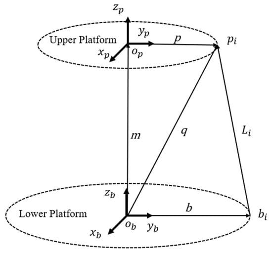
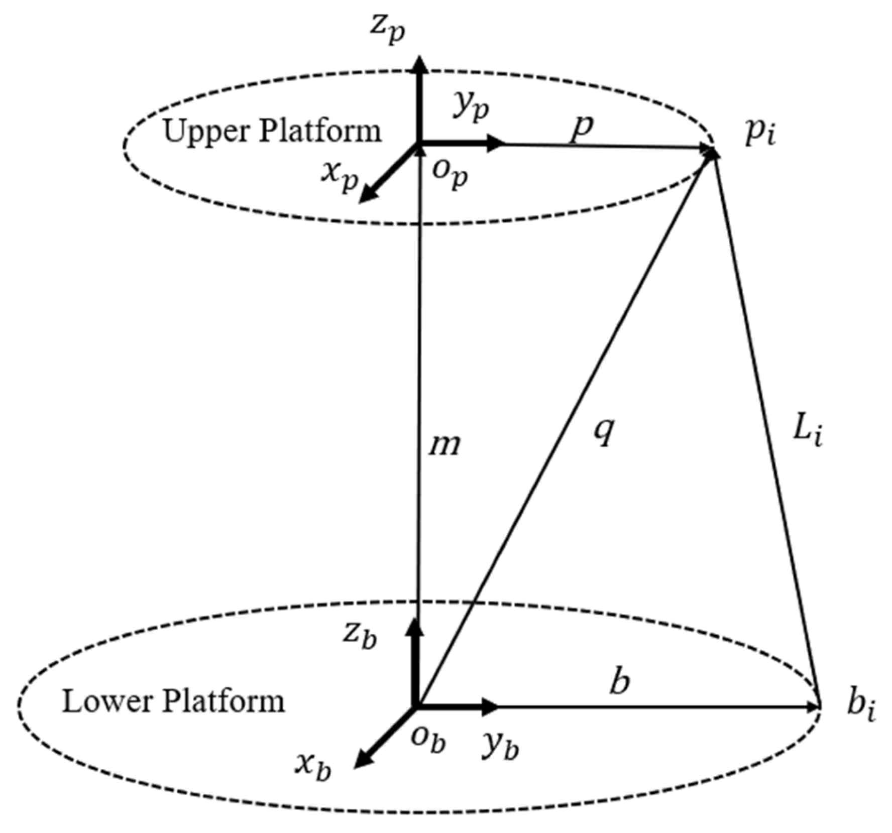
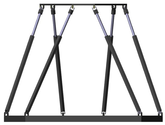
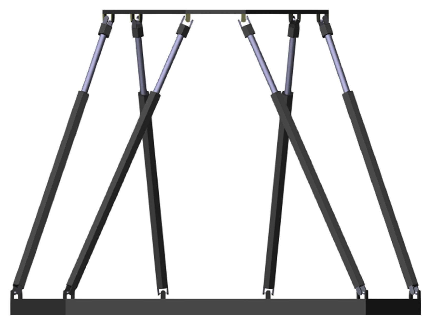
For a vehicle leveling system, it is necessary to investigate how to maintain the leveling platform at level when the vehicle’s attitude changes. The available data is the platform’s pose, while the actual control variable is the length of the drive rods; therefore, this paper addresses the inverse kinematics problem. The Stewart platform has a symmetrical structure, and the motion characteristics of each drive rod are identical. Thus, it suffices to perform a kinematic analysis on just one of the drive rods, as shown in Figure 1.
Figure 1.
Kinematic principle diagram.
For the inverse kinematics problem, we need to determine the extension amount and retraction of the drive rod :
where represents the extension of the -th drive rod; represents the initial length of the i-th drive rod; is the length vector of the i-th drive rod. The relationships between these vectors are as follows:
In the equation, represents the vector from the center point of the lower platform to the Hooke joint on the upper platform; represents the vector from the center point of the lower platform to the Hooke joint on the lower platform. In Figure 1, the coordinate vector of in the coordinate system must be transformed to the coordinate system using a rotation matrix. Therefore, the vector equals:
2.2. Dynamic Model
The nominal dynamic model of the Stewart platform provides a basis for designing the equivalent control term in the sliding mode framework. For the Stewart platform, its dynamic model can be expressed as:
where is the generalized coordinate vector; expresses the generalized force that acts in the six generalized coordinate directions ; is the total generalized inertia matrix of the platform; is the total Coriolis and centrifugal force matrix; and is the total gravitational moment.
represents the aggregate uncertainties, which includes unmodeled dynamics, friction forces, and external disturbances. In Equation (5), , , and denote unmodeled dynamics, denotes frictional forces, and denotes external disturbances.
Assumption: is bounded, i.e., there exists an unknown constant such that .
In the actual control process, to facilitate the implementation of the control law, Equation (4) needs to be transformed into joint space. Let denote the velocity vector at the upper hinge point; Let denote the extension velocity of the leg; the relationship between the velocity vector at the upper hinge point and the leg drive velocity vector is given by:
where is the Jacobian matrix from the leg drive velocity vector to the upper hinge point velocity vector. The transformation relationship between the upper hinge point velocity vector and the generalized velocity vector is:
where is the Jacobian matrix from the velocity vector at the upper hinge point to the generalized velocity vector.
From Equations (6) and (7), the relationship between the leg drive velocity and the generalized velocity vector is given by:
where expresses the Jacobian matrix from the leg velocity vector to the generalized velocity vector. Therefore, the relationship between the actual input force and the generalized force F is: . This yields the following dynamic model for the Stewart platform:
where expresses the actual driving force applied to the leg. From Equation (8), we obtain:
Substituting this into Equation (9) yields:
2.3. Dual-Platform Leveling Control Model
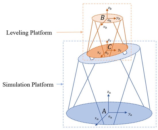
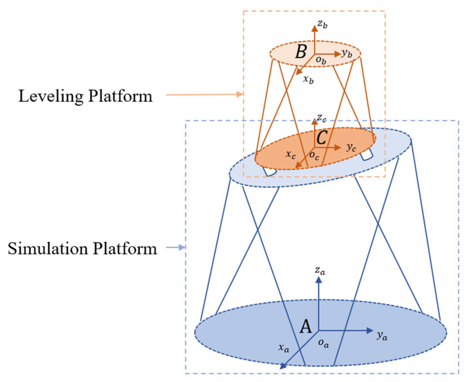
Under laboratory conditions, one Stewart platform acts as the road condition simulation platform, while another Stewart platform acts as the leveling platform. The principle of the Stewart platform leveling algorithm is shown in Figure 2. Given that: the coordinate system of the lower platform of the simulation platform is the world coordinate system A; the coordinate system of the lower platform of the leveling platform is the simulation coordinate system C(), which simulates the vehicle body pose signal; and the coordinate system B() of the upper platform of the leveling platform is fixed relative to the world coordinate system A. Solution: Determine the pose of coordinate system B relative to coordinate system C, which serves as the control input for the leveling platform. This ensures that the upper platform of the leveling platform remains stationary in the world coordinate system.
Figure 2.
Principle of Stewart platform leveling algorithm.
The formula for transforming the coordinates of a point between different coordinate systems is:
is the coordinate of point in coordinate system A. is the coordinate of point in coordinate system C. is the rotation matrix from coordinate system C to coordinate system A, describing the direction cosines of the three axes of coordinate system C in coordinate system A. is the coordinate of the origin of coordinate system C in coordinate system A. The objective of this paper is to determine , that is the coordinate of point in coordinate system C. Transform the above formula:
Since the rotation matrix is an orthogonal matrix, its inverse is equal to its transpose:
Apply this formula to find the coordinates of point in the C coordinate system
3. Design of a Non-Singular Terminal Sliding Mode Controller Based on RBF Neural Networks
3.1. Controller Design
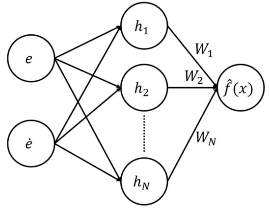
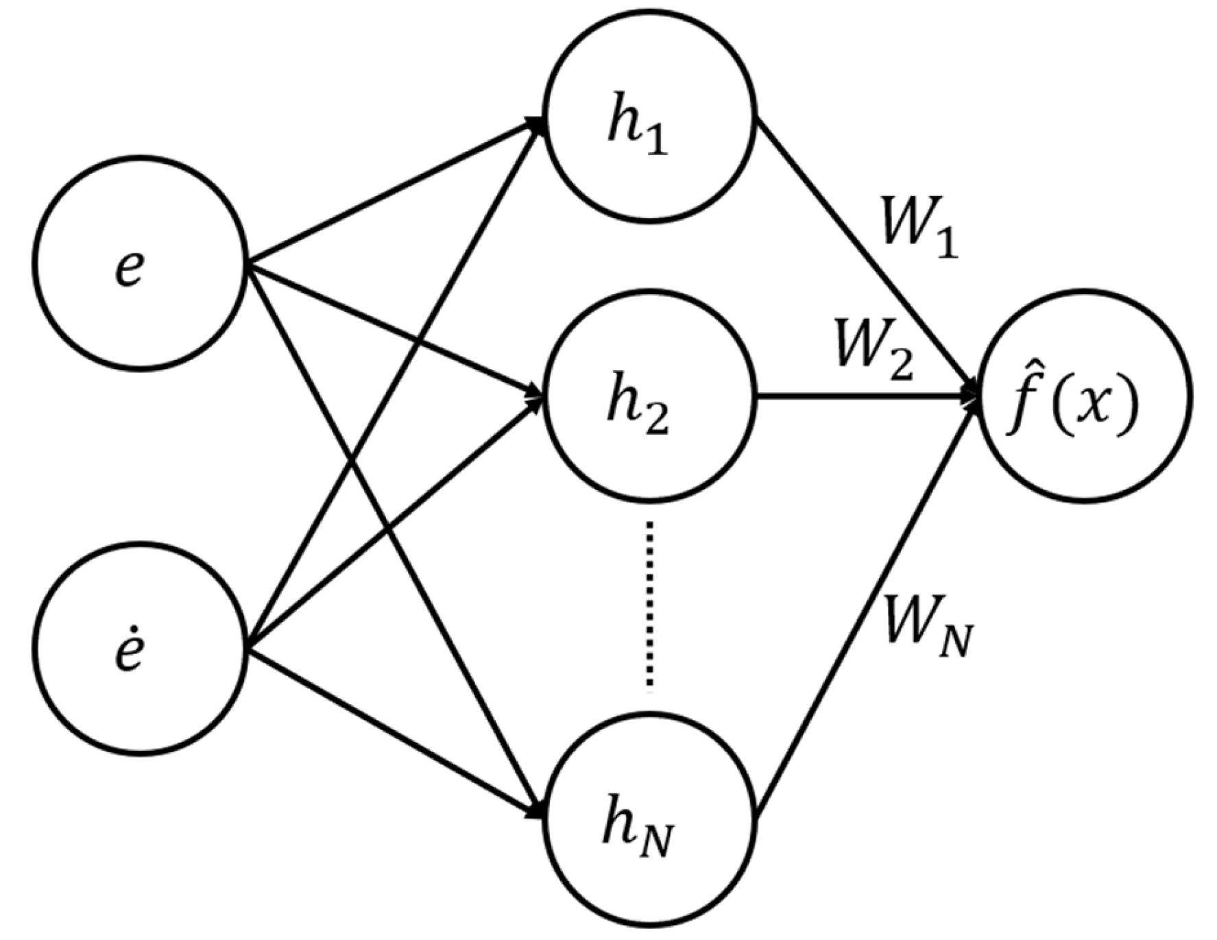
The RBF neural network consists of an input layer, a hidden layer, and an output layer, as shown in Figure 3. The RBF neural networks are used to approximate the aggregate uncertainties of the system.
Figure 3.
Schematic Diagram of the RBF Neural Network Structure.
In the i-th joint space, the output of the RBF neural network is:
Here, is the input vector to the network, is the estimated weight matrix of the neural network, is the number of hidden layer nodes, and is the Gaussian basis function vector. The j-th basis function is defined as:
Here, represents the center of the Gaussian basis function and represents the width of the base.
According to the universal approximation theorem, there exists an optimal weight vector such that , where is the approximation error satisfying , being a known constant. The weight estimation error is defined as .
Define the tracking error:
To avoid singularities, Feng [17] proposed a sliding surface with swapped variable positions, using the following non-singular terminal sliding surface:
Here, , , and .
Differentiate with respect to the sliding surface:
Substituting the system dynamics yields:
The convergence rate is designed to be
The control law design based on the RBF neural networks is:
Here, is the linear gain; is the switching gain, used to compensate for RBF approximation errors and residual disturbances, and must satisfy ; is the sign function.
Adaptive Weighting Law for RBF Neural Networks:
Here, denotes the learning rate matrix.
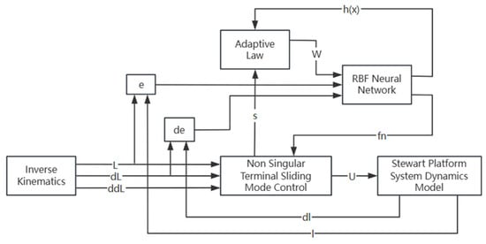
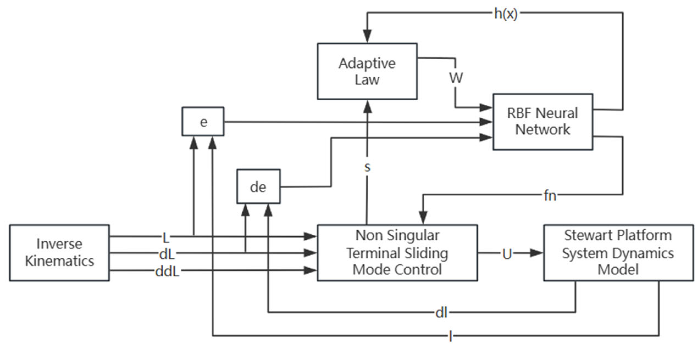
Figure 4 shows the schematic diagram of a non-singular terminal sliding mode controller based on an RBF neural network, where represents the output value of the RBF neural network.
Figure 4.
Non-Singular Terminal Sliding Mode Controller Based on RBF Neural Networks.
3.2. Controller Simulation
Road conditions are simulated using a random curve, which is composed of four superimposed sine waves. By limiting the amplitude and frequency of the sine functions, the random curve achieves a maximum amplitude of ±10 degrees and a maximum period of 5 s. The rules for generating random curves are as follows:
A visual model of the platform’s multibody dynamics was built using the Multibody module in MATLAB R2025a Simulink, as shown in Figure 5.
Figure 5.
Visualization Model of Multi-Body Dynamics on the Stewart Platform.
The dynamic model parameters extracted from the visualization model shown in Figure 5 are shown in Table 1.
Table 1.
Platform dynamics model parameters.
Since the parameters are the same for all six joints, configure the controller parameters for a single joint. Parameters for the non-singular terminal sliding mode controller: Sliding surface gain . , , . The parameters for the non-singular terminal sliding mode controller based on the RBF neural network are: initial network weights , number of hidden layer nodes , adaptive learning rate , , , , . Global scaling factor . The global scaling factor is primarily used to adjust the coverage of the input space and the width of the basis functions in an RBF neural network to match the magnitude of the actual error signals in the system.
The width of all nodes is set to the same constant:
The center is selected using a regular grid within the expected operating range of the input space. Based on the expected range of the error signal, we construct a grid with a step size of 0.2 within the interval [−1, 1].
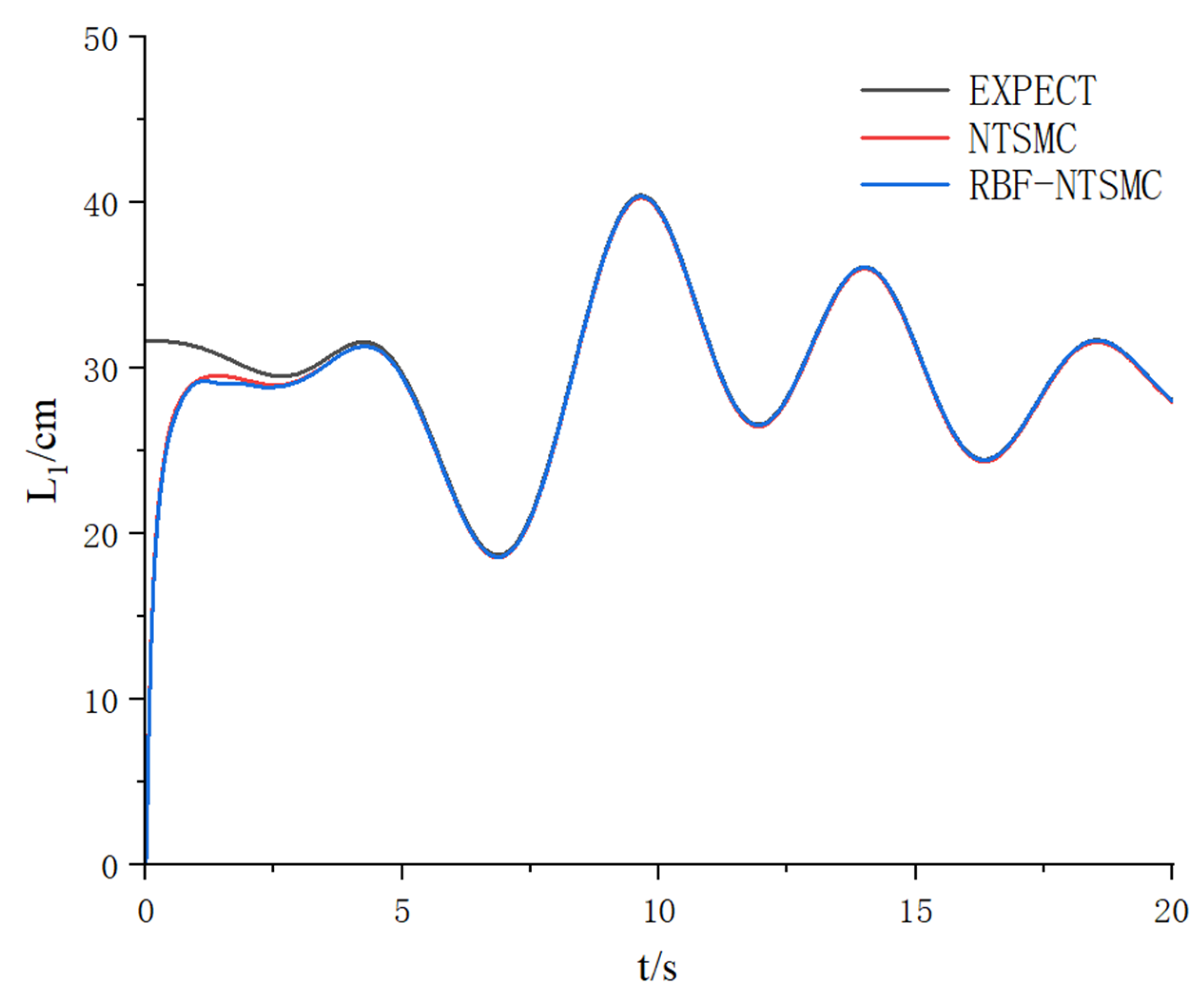
To comprehensively evaluate the performance of the non-singular terminal sliding-mode control strategy based on RBF neural networks proposed in this paper, simulation data in joint space for a Stewart platform were extracted. By comparing the traditional non-singular terminal sliding-mode control with the RBF neural network-based non-singular terminal sliding-mode control method proposed in this paper, quantitative and qualitative analyses were conducted in terms of trajectory tracking accuracy and control input smoothness to verify the superiority of the neural network approximation mechanism.
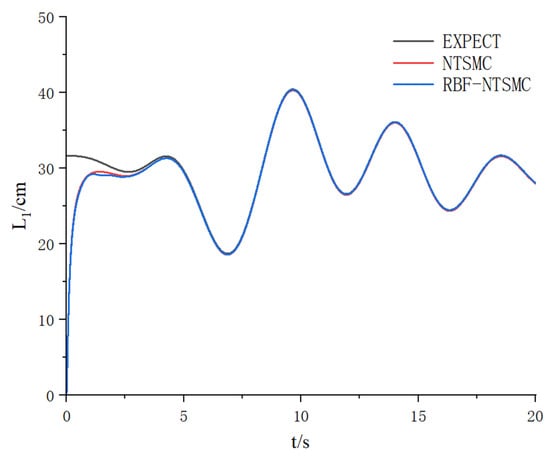
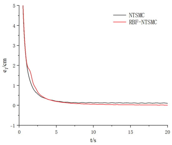
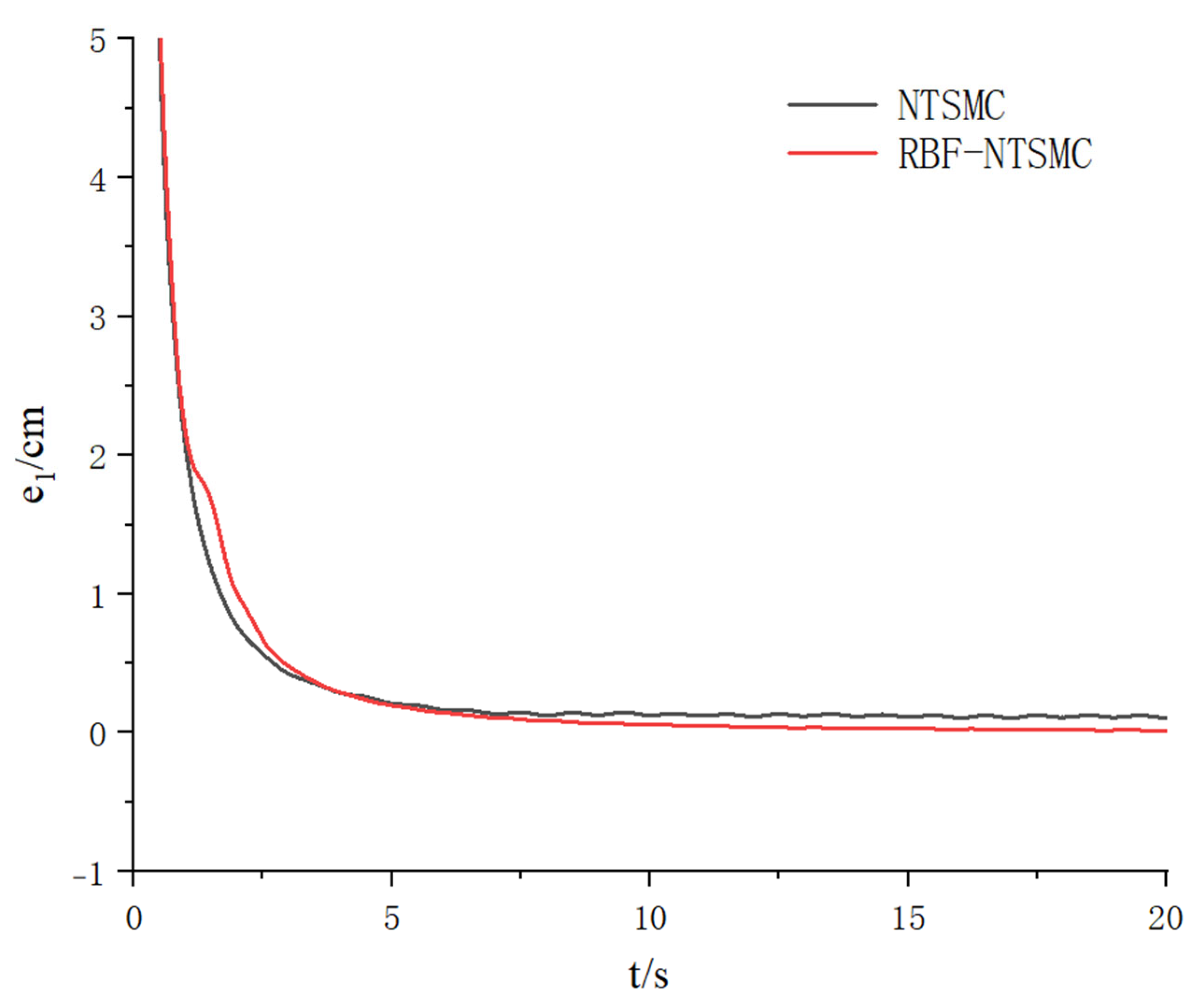
The length curve and length error of leg 1 are shown in Figure 6 and Figure 7. Ten seconds into the simulation, the tracking error of RBF-NTSMC primarily fluctuates within ±0.02 cm, whereas the error range of NTSMC fluctuates around ±0.15 cm.
Figure 6.
Length of Leg 1.
Figure 7.
Length Deviation of Leg 1.
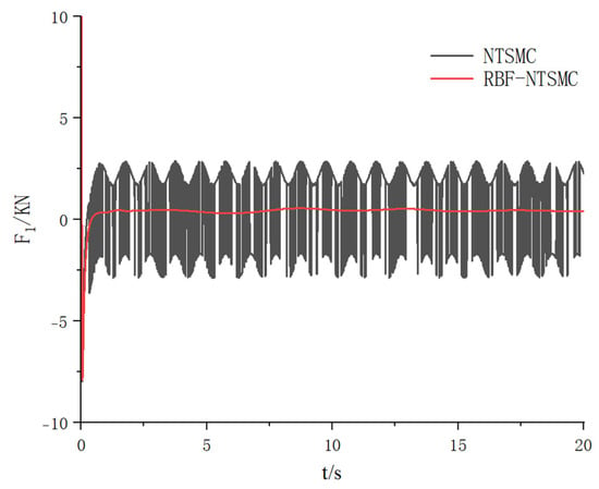
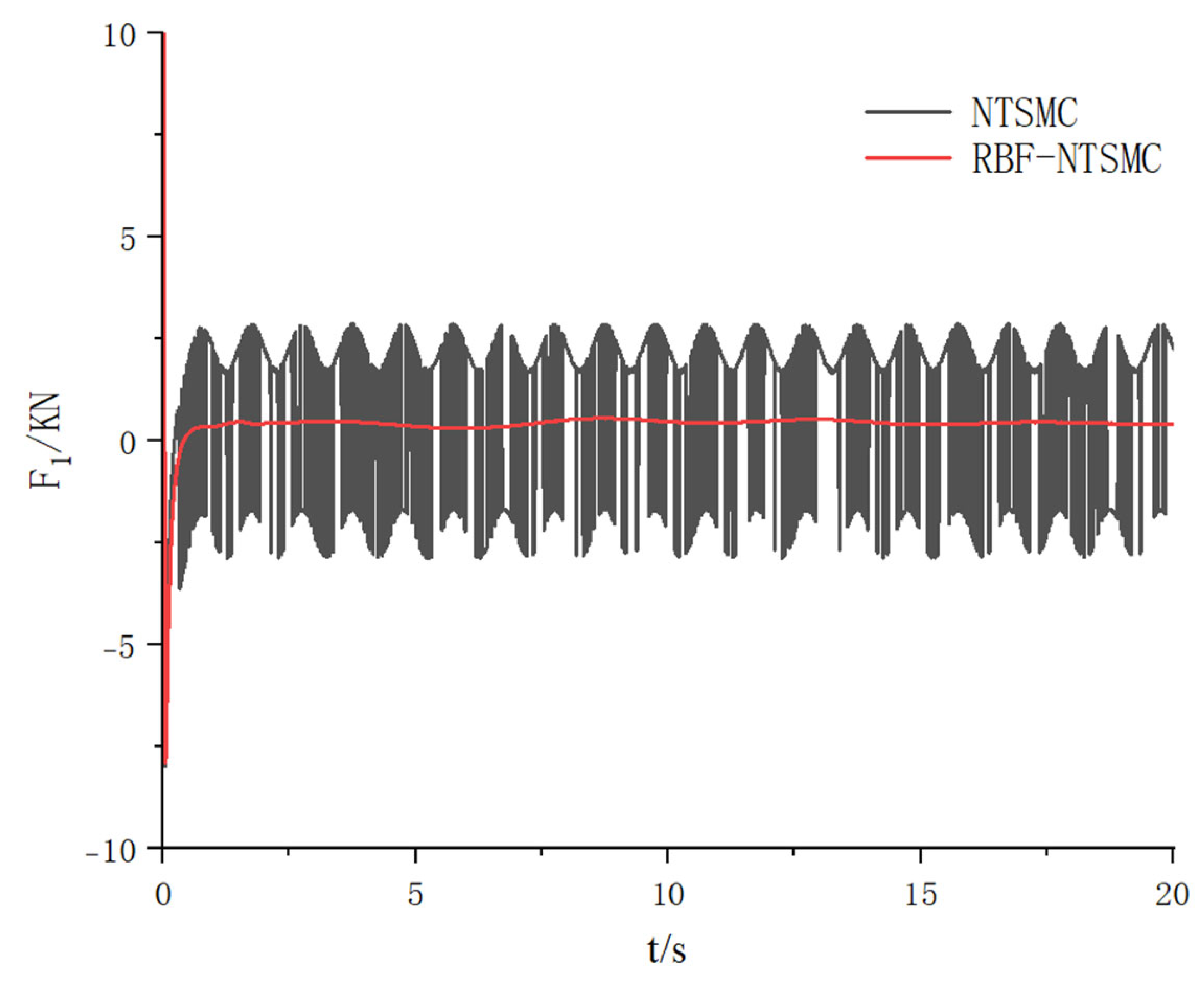
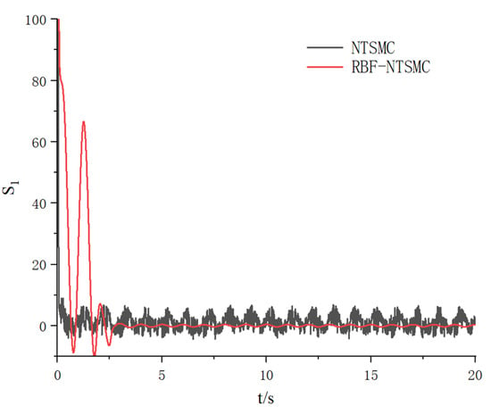
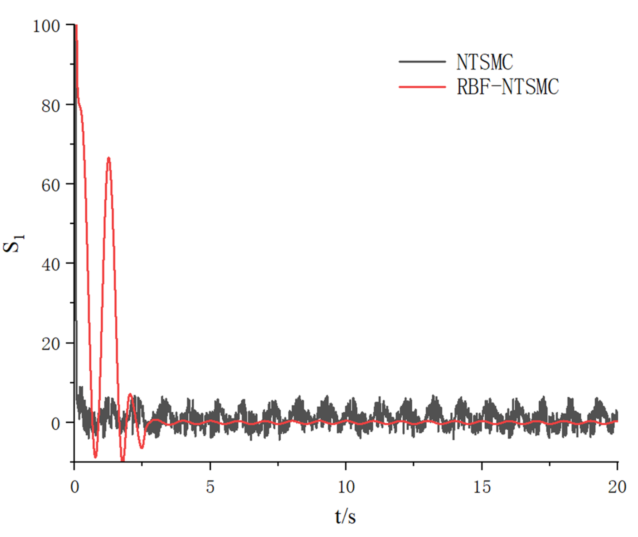
The drive force curve for leg 1 is shown in Figure 8. The NTSMC signal exhibits distinct high-frequency sawtooth oscillations, which result from frequent switching of the sign function to maintain the sliding surface , the peak fluctuation of the control force is approximately 2700 N. In contrast, the RBF-NTSMC signal curve is smooth, with significantly reduced high-frequency components, and the peak fluctuation is reduced to within 500 N. NTSMC requires a large switching gain to account for all uncertainties, which directly leads to severe chattering. RBF-NTSMC compensates for lumped uncertainties through the continuous function , with the switching term needing to handle only minor approximation errors. Therefore, while ensuring robustness, it significantly reduces the switching gain, thereby suppressing chattering at its source.The sliding mode surface for leg 1 is shown in Figure 9.
Figure 8.
Drive Force of Leg 1.
Figure 9.
Sliding Mode Surface for Leg 1.
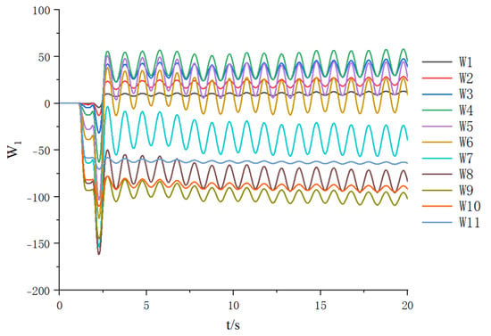
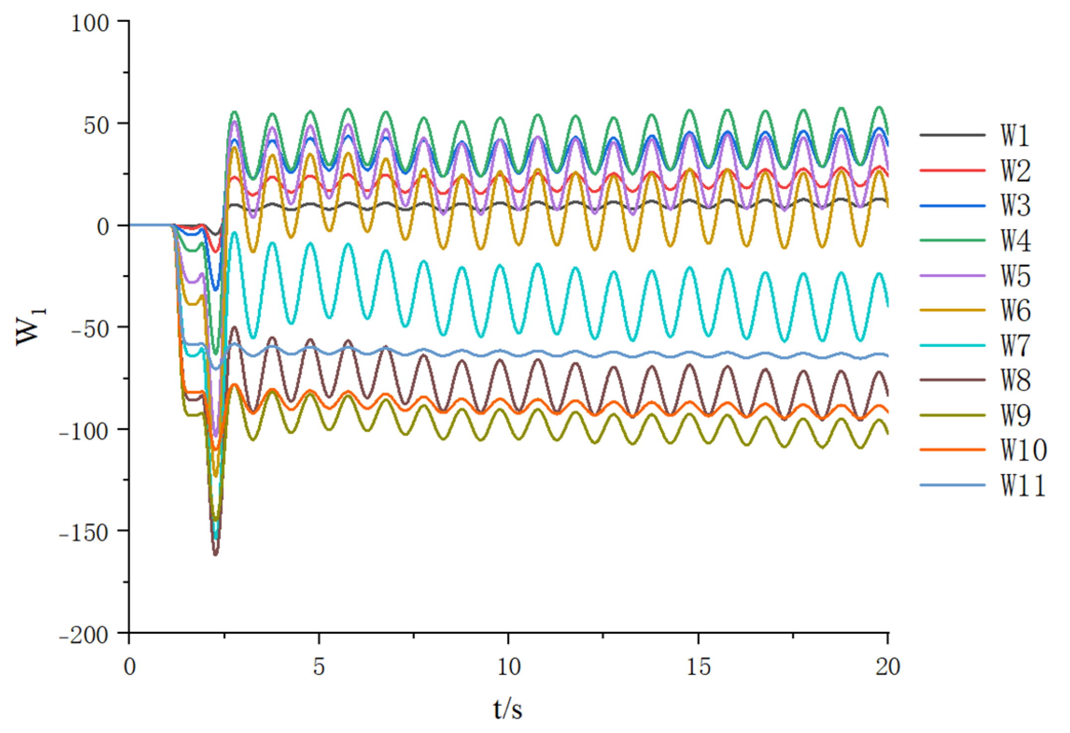
Figure 10 shows the online learning process of the RBF neural network’s partial weights . It can be observed that during the initial simulation phase, the weights undergo significant fluctuations, indicating the network is rapidly learning the system’s dynamic characteristics and initial error. As the tracking error diminishes, the weights gradually stabilize within a bounded range. This validates the effectiveness of the adaptive law, demonstrating the neural network’s capability for real-time online identification of aggregate uncertainties.
Figure 10.
Neural Network Weights for Leg 1.
4. YOLO11n-Seg-Based ORB-SLAM3
4.1. Improved Solution
The YOLO11n-Seg model is a version of the YOLO (You Only Look Once) object detection framework specifically optimized for real-time instance segmentation tasks. Building upon the efficient architecture of the YOLO series, it further integrates advanced instance segmentation mechanisms, enabling both object detection and pixel-level segmentation to be performed simultaneously in a single forward pass. The parameters of the YOLO11n-Seg model and the pre-training parameters are shown in Table 2.
Table 2.
YOLO11n-Seg Model and Training Parameters.
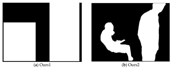
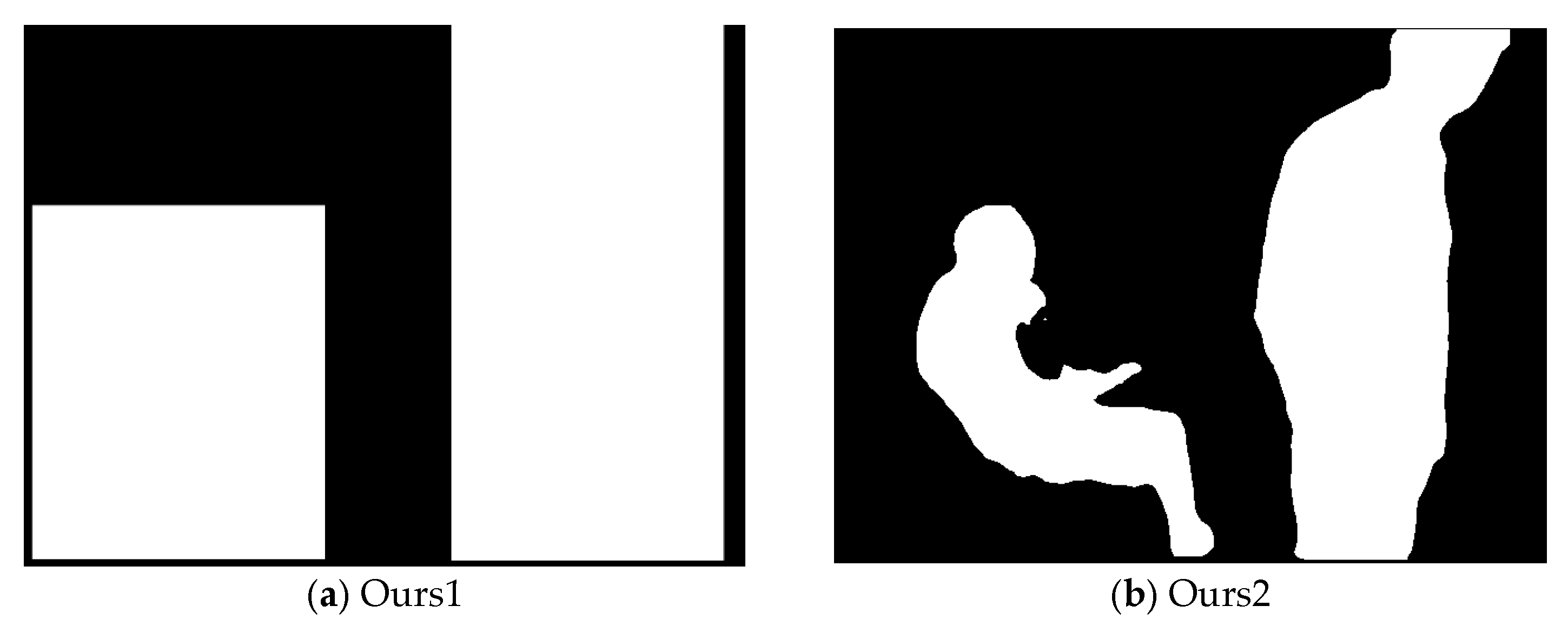
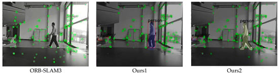
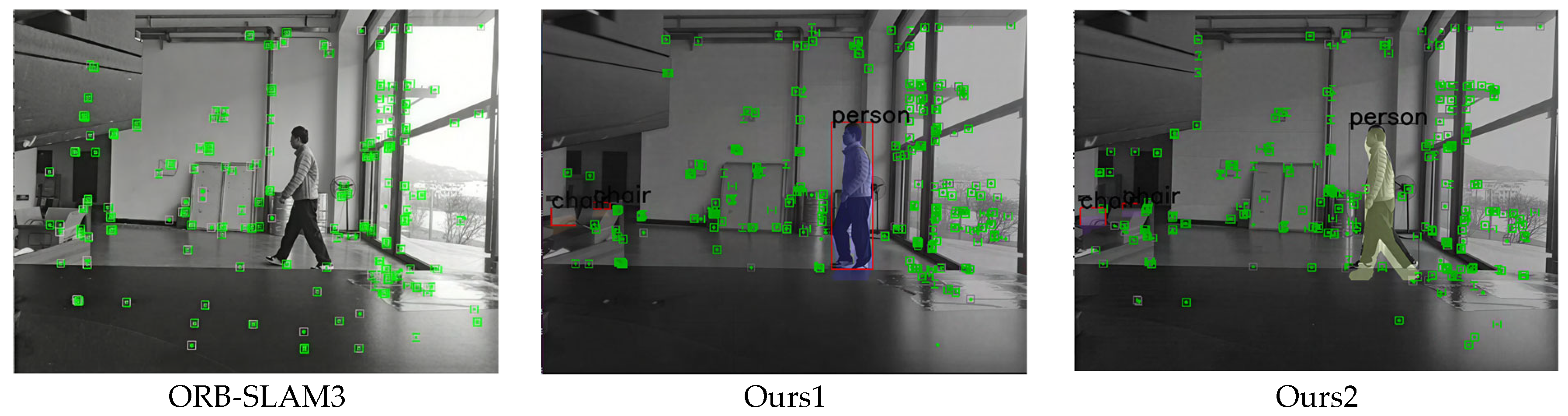
ORB-SLAM3 is susceptible to interference from dynamic feature points, which reduces the accuracy of pose estimation. Some YOLO-based ORB-SLAM3 methods address this issue by removing all feature points located within the bounding boxes of detected dynamic objects. However, this approach also filters out valid static feature points within the bounding boxes. This paper adopts YOLO11n-Seg as the source of semantic information. YOLO11n-Seg outputs the class label, confidence score, bounding box, and 32 mask coefficients for each detected instance. The post-processing stage first filters out detection results with confidence scores below 0.5. For instances with sufficient confidence, a segmentation mask is generated by linearly combining their mask coefficients with the prototype mask only if the category belongs to a predefined dynamic category. This mask is then upscaled and thresholded to restore it to a binary mask at the original image resolution. The masks of all dynamic instances are fused to produce the final binary map of dynamic regions, where pixel values in dynamic regions are set to 255 and those in static regions are set to 0. The algorithm using bounding box filtering (Ours1) is shown in Figure 11a. The algorithm using mask filtering (Ours2) is shown in Figure 11b. White expresses dynamic regions, and black expresses static regions. The processed mask is passed to the tracking thread of ORB-SLAM3. For each feature point detected in the current frame via the ORB feature extraction algorithm, its precise pixel coordinates in the image coordinate system are obtained. On the mask image, the pixel position corresponding to the feature point’s coordinates is located, and the grayscale value at that position is read. If the grayscale value of that pixel is 0, indicating that the feature point is located within a static background region, it is retained for subsequent inter-frame matching and pose estimation. If the grayscale value of that pixel is 255, indicating that the feature point is located within the contour of a dynamic object, it is classified as a dynamic feature point and discarded, thus excluded from any subsequent SLAM computation processes.
Figure 11.
Mask Diagram for Bounding Box Filtering and Mask Filtering.
In environments involving occlusion or rapid motion, false negatives or false positives may occur. False negatives result in dynamic points not being removed, affecting accuracy; false positives lead to static points being erroneously discarded. In experiments, we observed fewer false positives, which can be further reduced by employing high confidence thresholds.
4.2. Validation on the Dataset
The experimental setup utilized a computer configuration featuring a 12th Gen Intel® Core™ i5-12600KF processor (3.70 GHz) (Intel, Santa Clara, CA, USA), an NVIDIA GeForce RTX 4060 graphics card (8 GB) (NVIDIA, Santa Clara, CA, USA), and 32.0 GB of RAM. The software environment ran on the Ubuntu 22.04 operating system. To validate the effectiveness of the dynamic point removal algorithm, experiments were conducted on the fr3 sequence from the TUM RGB-D dataset. This sequence includes the sitting sequence for low-motion scenes and the walking sequence for high-motion scenes. Both sequences exhibit four camera motion patterns: static, xyz, half-sphere, and rpy. This paper selects motion patterns such as sitting_static, walking_static, walk_halfsphere, walking_xyz, and walking_rpy for testing, evaluating the camera’s pose estimation capability in dynamic environments.
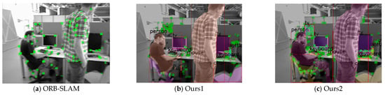
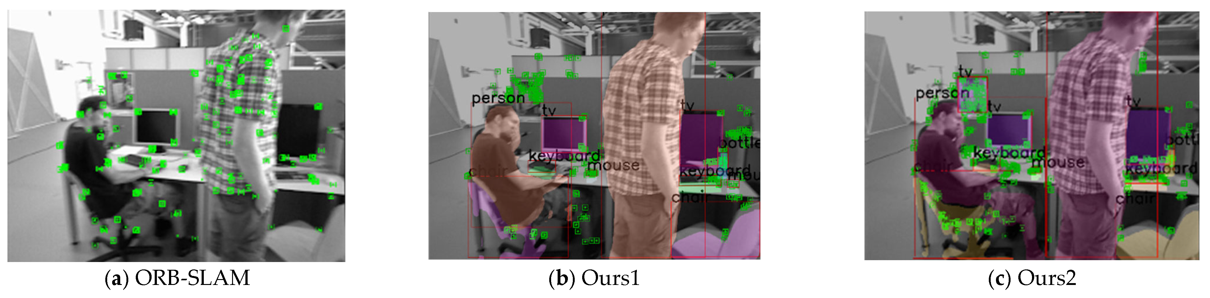
Figure 12 compares the performance of ORB-SLAM3 and the improved algorithm proposed in this paper in terms of feature point recognition in dynamic environments using the TUM-RGBD dataset. Ours1 filters out all moving feature points within the bounding box, while Ours2 filters out feature points within the masked regions of moving objects in the object bounding box, thereby retaining static feature points within the object bounding box.
Figure 12.
Feature Point Removal Effectiveness in Three-Axis Translation Scenarios.
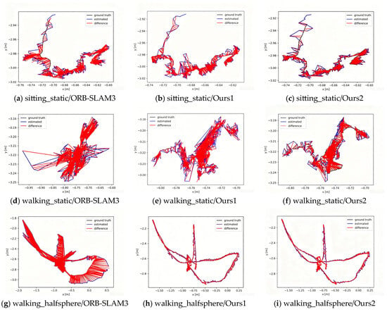
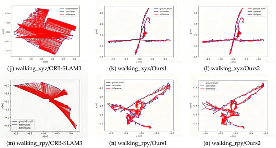
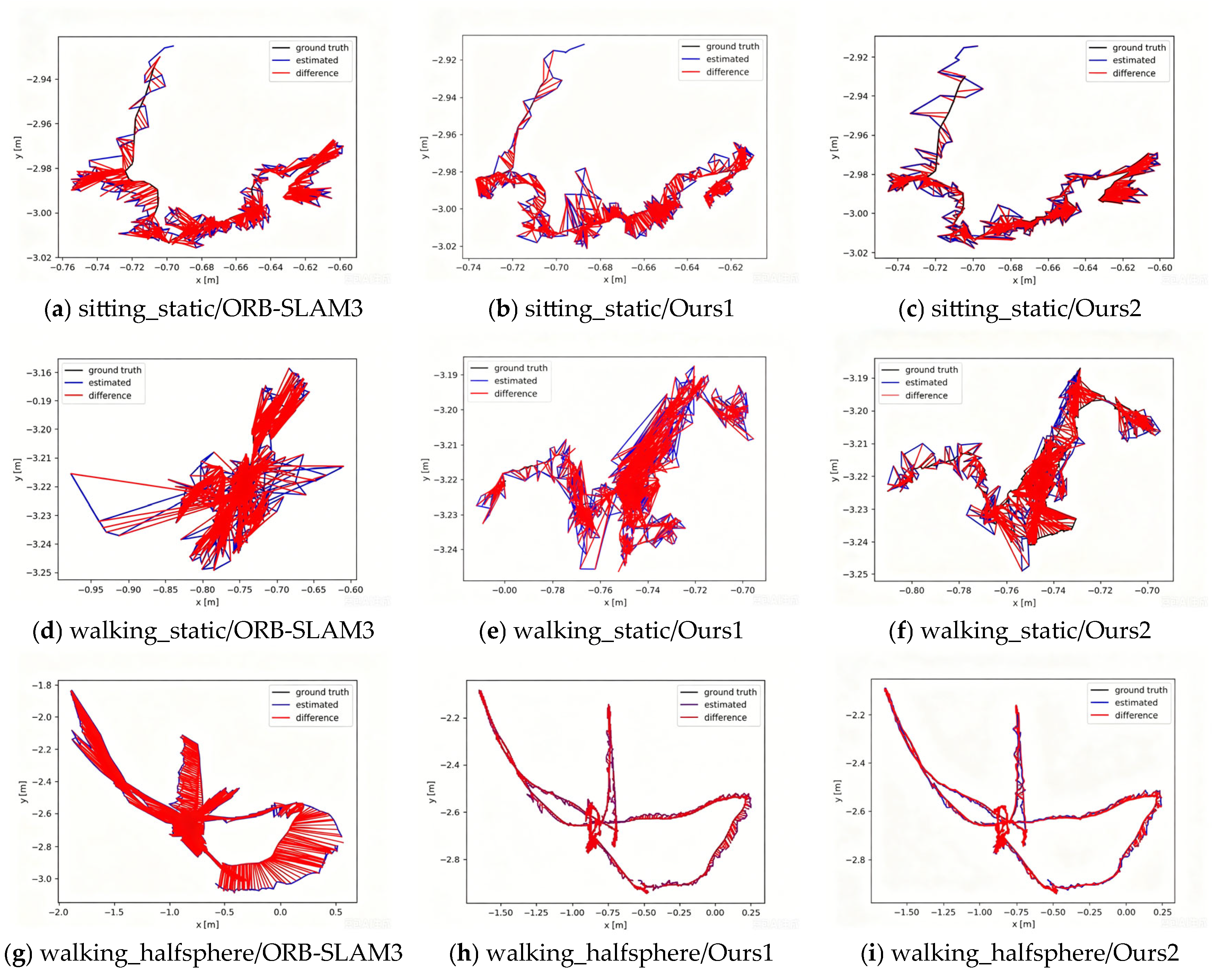
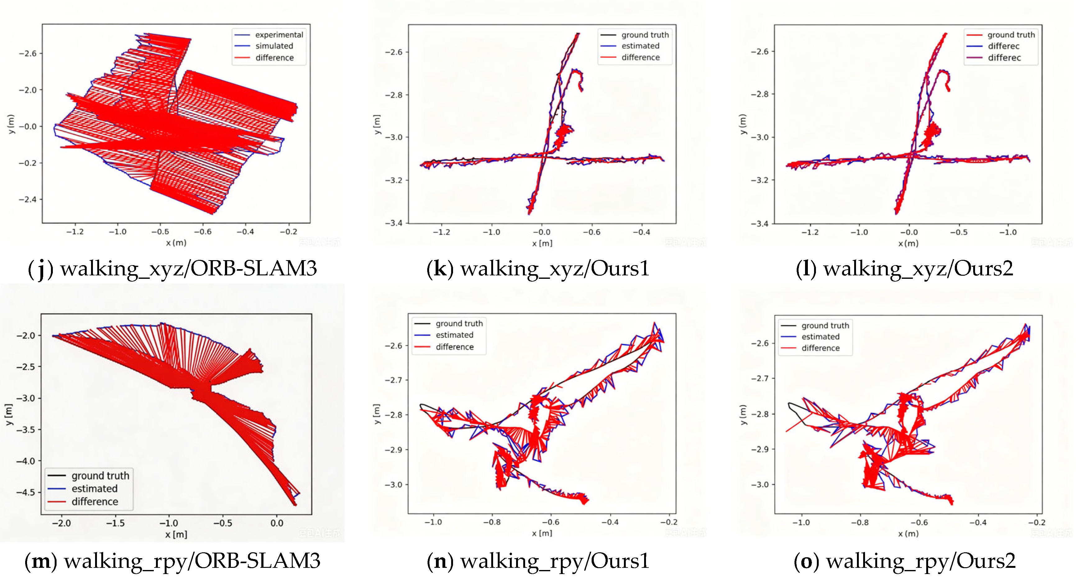
Trajectory evaluation was performed using the evaluate_ate.py tool; the absolute trajectory error is shown in Figure 13. Each sequence was run five times, and the mean and standard deviation were calculated. Additionally, we have included comparison results with RDS-SLAM. The test results in Figure 13 demonstrate that the proposed algorithm effectively suppresses interference through the dynamic feature point removal module, resulting in a significant reduction in SLAM pose estimation error. As shown in Table 3, absolute trajectory error is measured using root mean square error (RMSE) and standard deviation. Table 3 summarizes the absolute trajectory error RMSE and standard deviation for all evaluated algorithms. In static and low-dynamic sequences, the proposed Ours2 method achieved errors of 0.0073 m and 0.0072 m, respectively, surpassing the baseline ORB-SLAM3. In contrast, RDS-SLAM exhibited significant degradation in the walking_static sequence with an error of 0.1468 m. Under high-dynamic interference, ORB-SLAM3 failed with errors exceeding 0.4 m, while Ours2 maintained accuracy within 0.0256 m, reducing error by over 90 percent compared to the baseline. Although RDS-SLAM showed slightly lower error in the walking_rpy sequence, Ours2 demonstrated more consistent performance across all scenarios. The advantage of the segmentation mask strategy in Ours2 over the detection box approach in Ours1 is evident in the walking_xyz sequence, where the error was optimized to 0.0120 m. Additionally, Ours2 maintained a standard deviation below 0.0144 m across all tests, confirming superior system stability. These results validate the effectiveness of the proposed dynamic point removal strategy in dynamic environments.
Figure 13.
Absolute Trajectory Error.
Table 3.
Root mean square error and standard deviation of absolute trajectory error.
Table 4 shows the tracking time. The tracking time of the proposed algorithm is higher than that of ORB-SLAM3. A direct runtime comparison between our method and RDS-SLAM is not possible due to the use of different GPU hardware. Nevertheless, the data in Table 4 suggest that our approach achieves a promising tracking time on an RTX 4060. Table 4 shows that our method achieves a per-frame tracking time of 20–30 ms on an NVIDIA RTX 4060. This measurement is broken down as follows: YOLOv11n-Seg inference takes 10–15 ms, ORB feature extraction takes 6–8 ms, and feature matching with pose optimization takes 6–10 ms. The YOLO inference and ORB extraction execute in parallel. However, the subsequent filtering, matching, and optimization steps require both outputs, necessitating thread synchronization and data transfer (2–4 ms overhead). The total time, therefore, reflects the sum of the slower parallel module and the sequential matching stage plus overhead, which consistently falls within the reported 20–30 ms range.
Table 4.
Tracking Time.
5. Experimental Section
5.1. Experimental Platform Setup
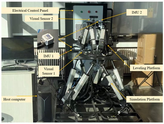
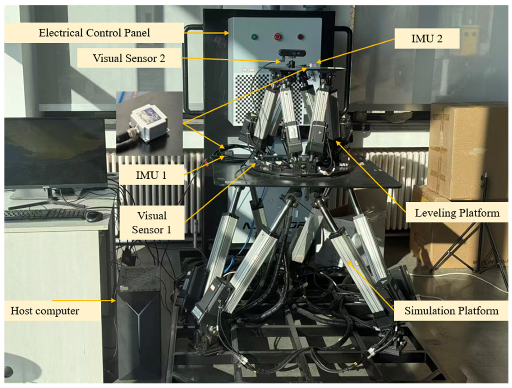
The leveling system used in the experiment is shown in Figure 14. Its main components include a host computer, an electrical control cabinet, a Simulation Platform, a leveling platform, an IMU, and a vision sensor. The vision sensor is an Orbbec Gemini 336L camera (Orbbec, Shenzhen, China). The IMU is the LPMS-IG1 from LP-RESEARCH. To ensure system safety, two Stewart platforms of different sizes were selected to serve as the vehicle pose simulation platform and the leveling platform, respectively, and were connected via threaded joints. The cameras are mounted on the upper surfaces of the two upper platforms, respectively.
Figure 14.
Pose leveling experimental device.
We did not fuse the data from the IMU and the camera. The IMU measures roll and pitch angles, while the camera measures pitch displacement. The IMU’s pose output frequency is 200 Hz. The camera’s pose output frequency is 30 Hz. The controller’s control signal output frequency is 20 Hz. To handle this frequency mismatch, we use a zero-order hold strategy: the control loop uses the most recent camera-based displacement estimate until a new estimate becomes available. This approach ensures deterministic timing and avoids introducing additional interpolation delays.
5.2. Analysis of Experimental Results
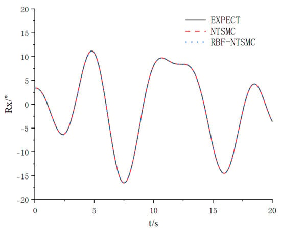
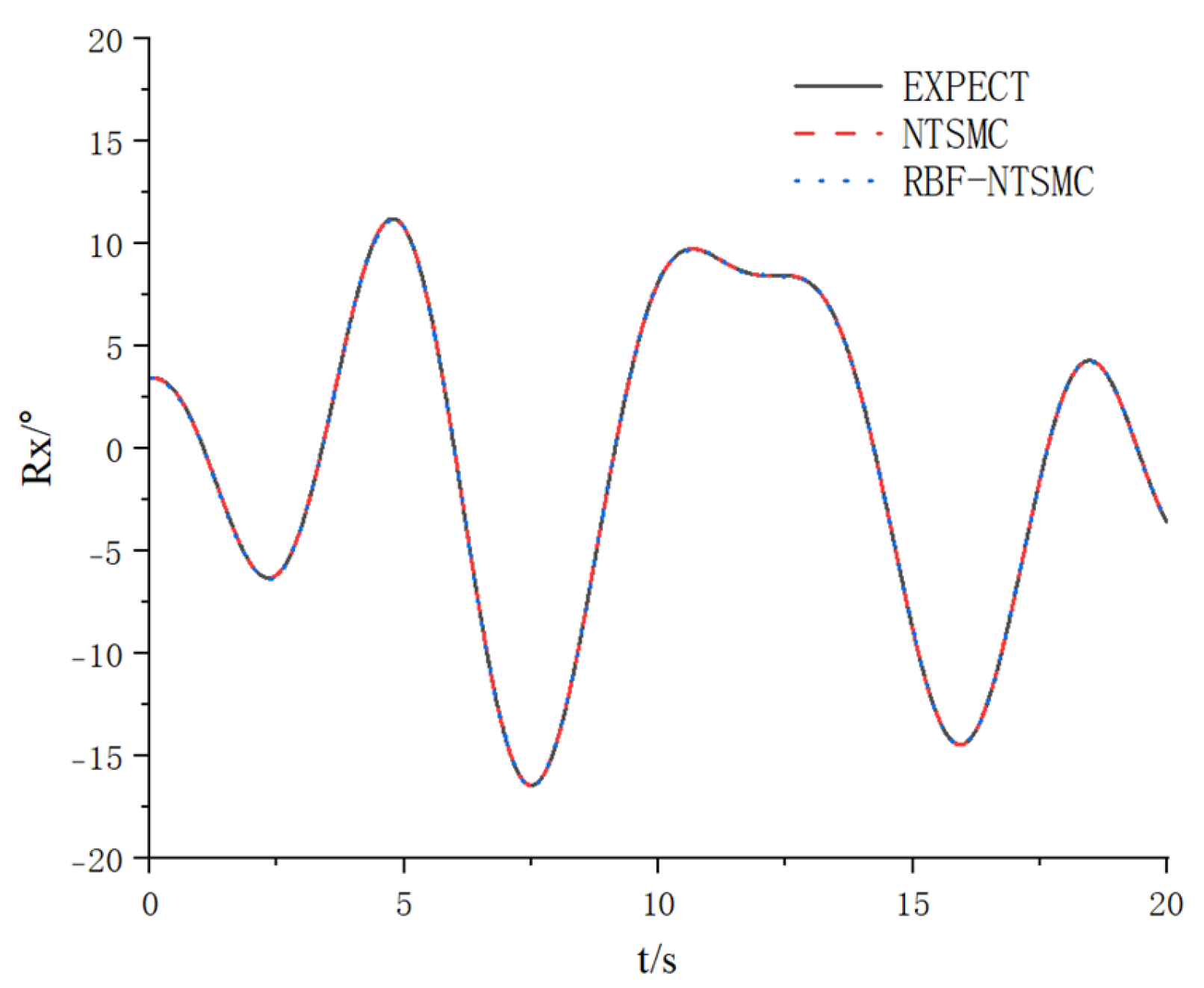
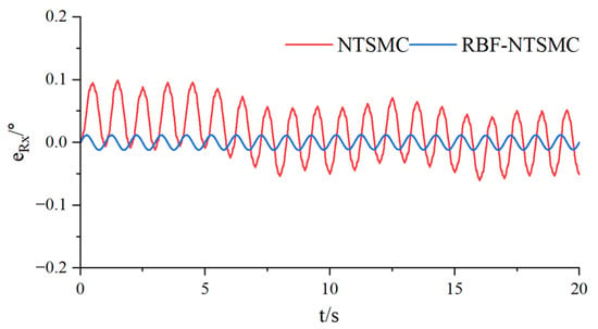
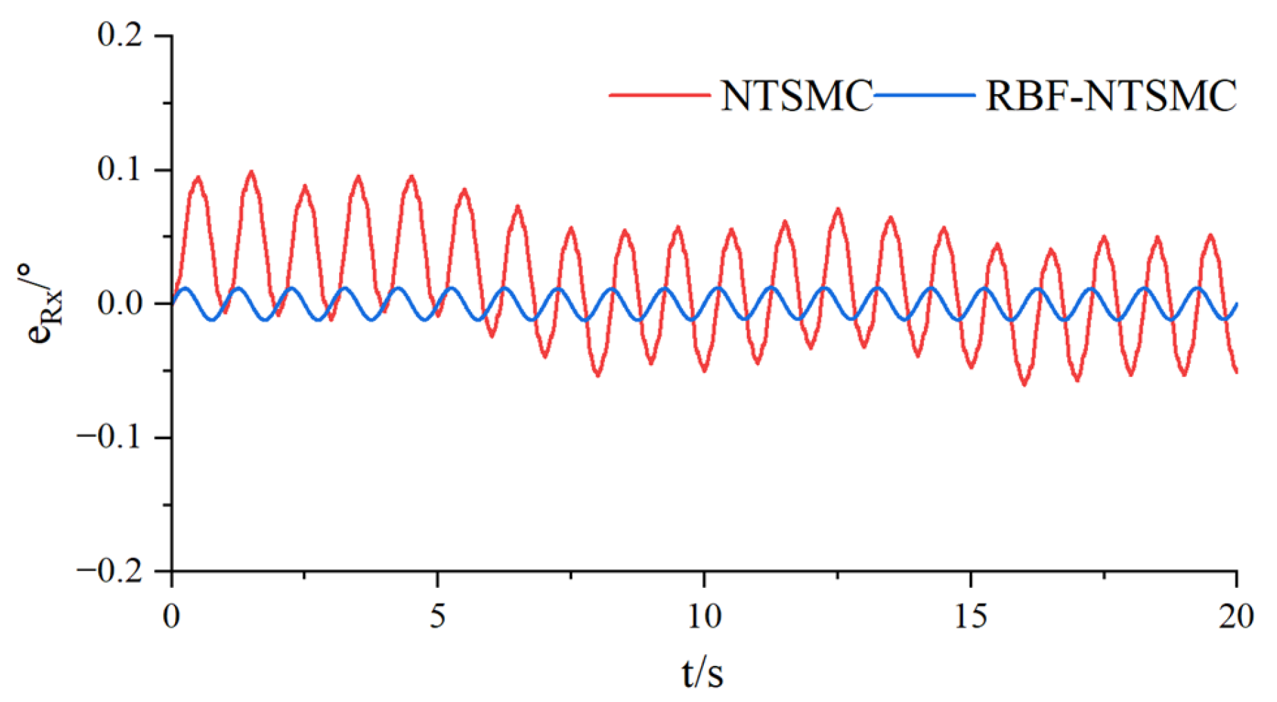
Control algorithm validation experiments were conducted on a simulation platform system, using an IMU to measure the actual orientation of the simulation platform. The roll angles and errors are shown in Figure 15 and Figure 16. The error magnitude for the NTSM control scheme was 0.1 degrees, while that for the RBF-NTSMC scheme was 0.01 degrees.
Figure 15.
Roll angle.
Figure 16.
Roll angle error.
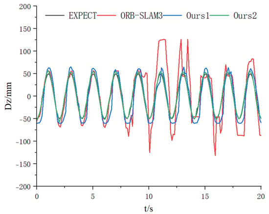
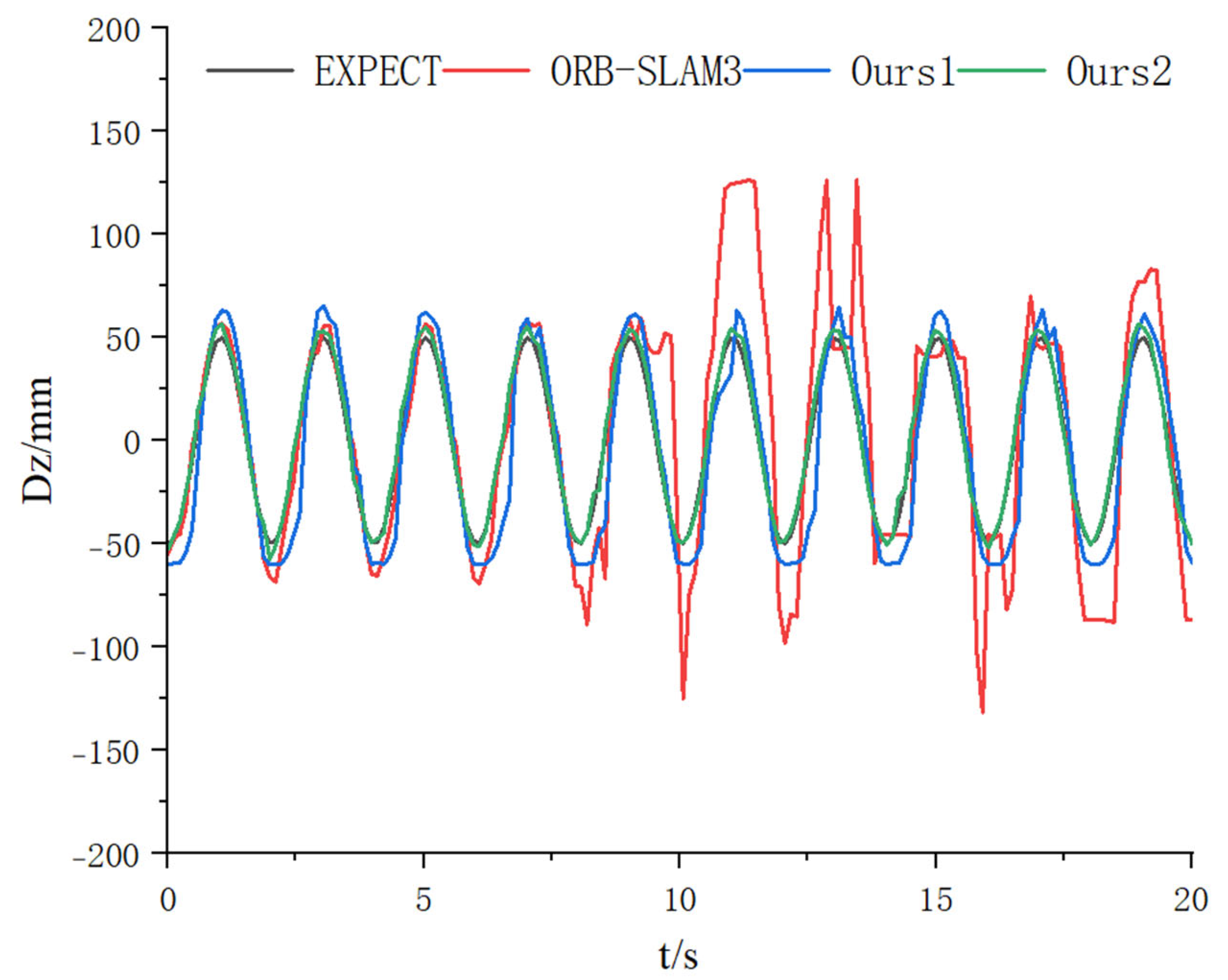
Next, we conducted an experimental validation of the pose estimation using visual sensors. We had the Stewart simulation platform perform a translational motion along the Z-axis, with a sinusoidal trajectory described by Dz = 50 sin (3.14t + 3.14) mm. and recorded the camera’s pose while running ORB-SLAM3 and the improved algorithm described in this paper.
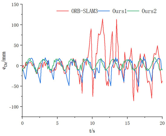
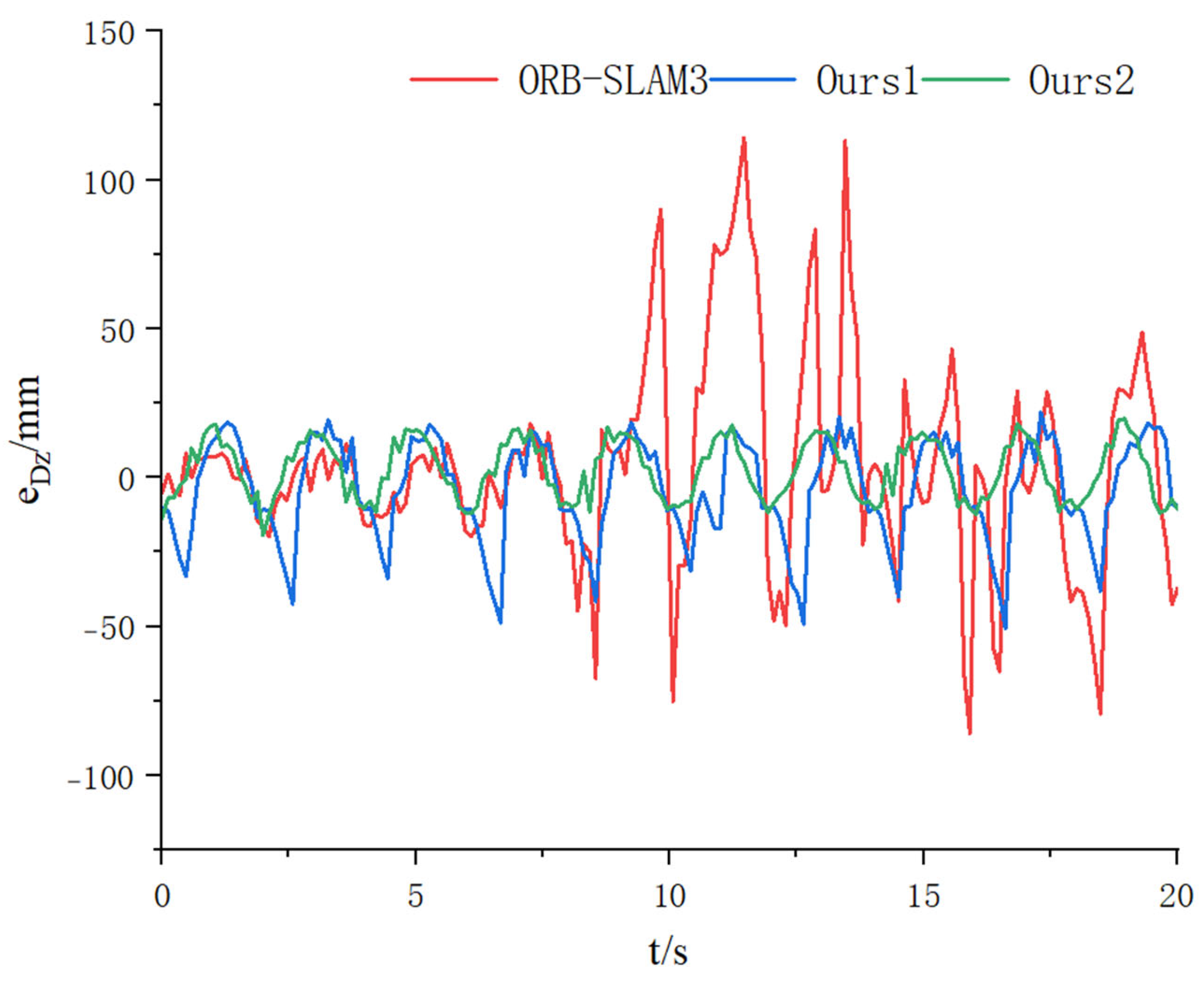
The results of feature point detection are shown in Figure 17. In this paper, the bounding box filtering algorithm was used to filter out all dynamic feature points within the bounding box, while the mask filtering algorithm was used to filter out feature points within the mask region of the dynamic object’s bounding box, thereby retaining the static feature points within the dynamic object’s bounding box. The pose estimation curves and estimation errors of the visual sensor are shown in Figure 18 and Figure 19. The pose curve of ORB-SLAM3 exhibits excessive errors at certain time points, with a mean absolute error of 21.83 mm. The algorithm using bounding box filtering in this paper achieves a mean absolute error of 14.35 mm, while the algorithm using Mask filtering achieves a mean absolute error of 9.15 mm.
Figure 17.
Feature point removal effect.
Figure 18.
Visual sensor pose estimation curve.
Figure 19.
Visual sensor pose estimation error.
The leveling experiment protocol is as follows: Simulated vehicle pose signals are input to the simulation platform, using the desired values shown in Figure 15 and Figure 18. The simulation platform simulates the vehicle’s roll and heave motions. Visual sensor 1 and IMU 1 acquire the pose signals of the simulation platform. The acquired pose signals are transmitted to the leveling platform. The leveling platform performs leveling control based on the dual-platform leveling control algorithm. Visual sensor 2 and IMU 2 collect the pose signals of the leveling platform.
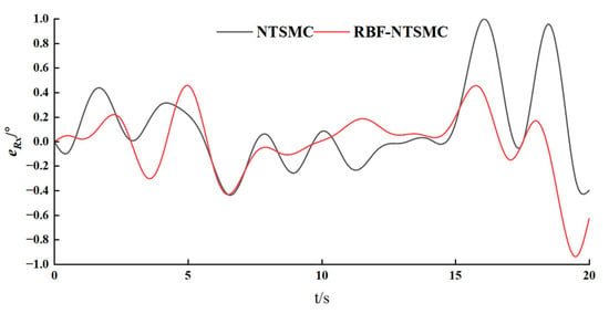
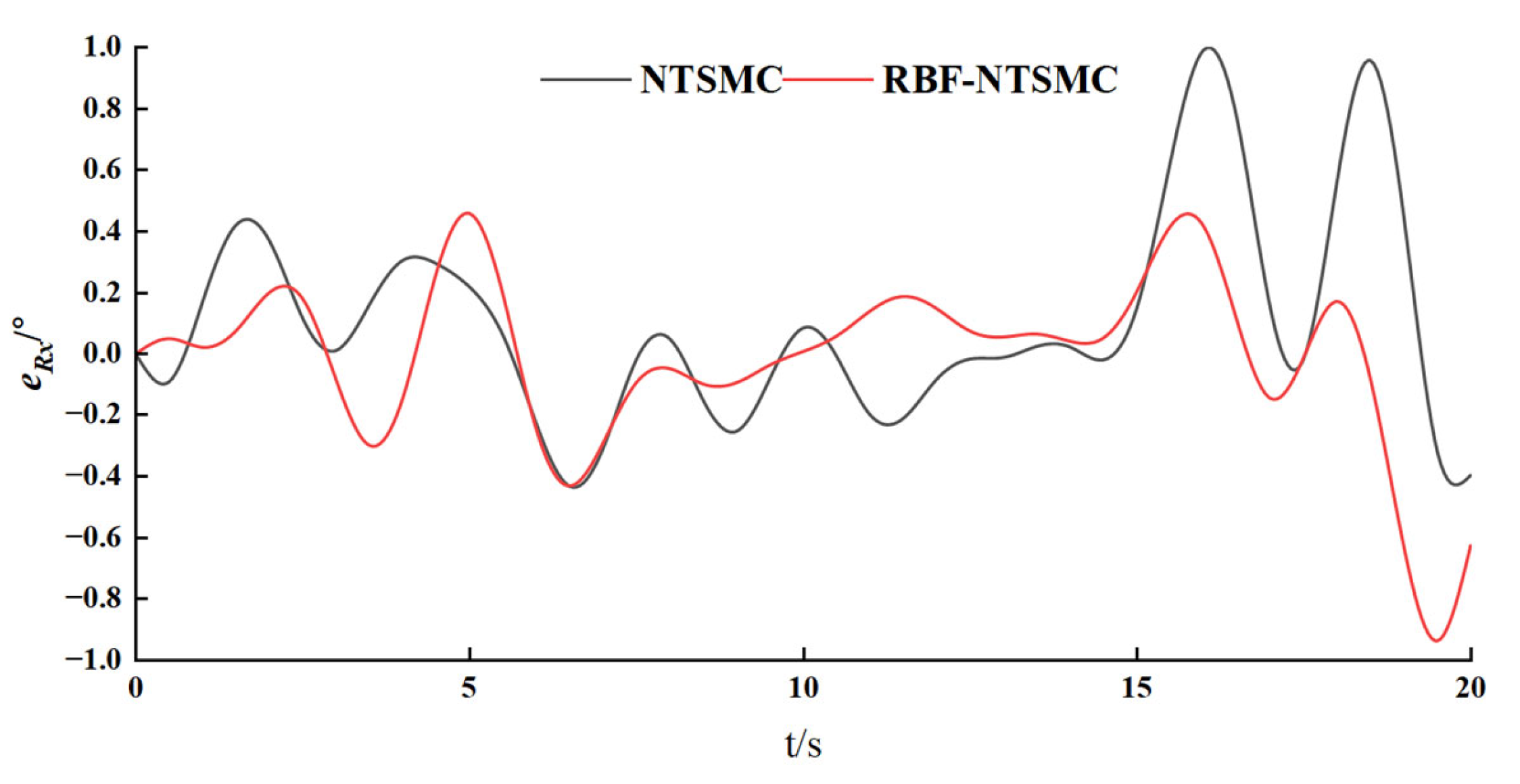
Figure 20 shows the leveling error in the roll angle of the leveling platform. Analysis of the roll angle leveling error reveals that the mean absolute error for the NTSM control scheme is 0.24 degrees, while that for the RBF-NTSM control scheme is 0.19 degrees. Although the maximum leveling error for both control schemes reaches 1 degree, they still meet practical application requirements.
Figure 20.
Roll angle leveling error of upper platform.
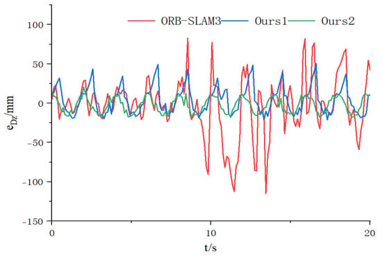
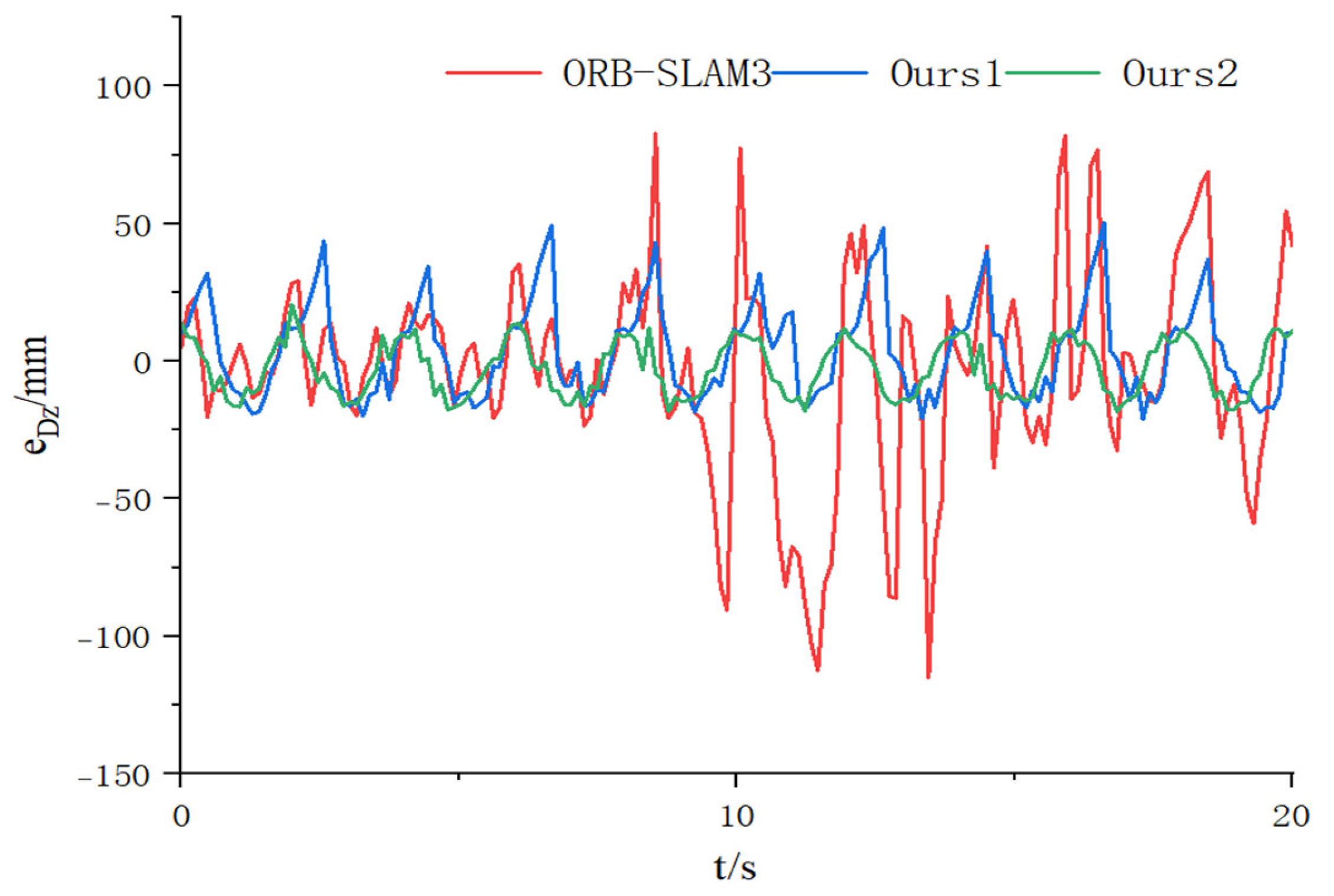
Figure 21 shows the leveling error resulting from the heave motion of the leveling platform. At this point, the control algorithm has a minimal impact on the leveling error; the primary source of error is the measurement error of the visual sensors. The maximum leveling error for ORB-SLAM3 is 115.07 mm, and the mean absolute error is 24.47 mm. The maximum leveling error of the algorithm using bounding box filtering in this paper is 51.36 mm; the mean absolute error is 14.37 mm; the maximum leveling error of the algorithm using mask filtering is 20.18 mm; the mean absolute error is 8.86 mm; the amplitude of the vehicle’s heave motion is 50 mm, and the amplitude of the leveling error is approximately 20 mm. The experimental results indicate that this control system can reduce the amplitude of the leveling platform’s heave motion by 60% relative to the amplitude of the vehicle body’s heave motion, thereby providing active leveling to counteract changes in the vehicle’s attitude.
Figure 21.
Heave motion leveling error of upper platform.
6. Conclusions
To address the safety concerns of non-autonomous casualties caused by changes in vehicle attitude when autonomous rescue vehicles operate on an unstructured road sur-face, this study proposes an active leveling control system based on the Stewart platform. The core innovations of this system lie in two aspects: First, at the leveling control level, a non-singular terminal sliding-mode control controller based on a radial basis function (RBF) neural network was designed. This controller utilizes the RBF neural network to approximate the aggregate uncertainties in real time, effectively enhancing the accuracy and robustness of the non-singular terminal sliding-mode control while reducing control input oscillations. Second, at the pose and attitude perception level, an improved ORB-SLAM3 algorithm is proposed. By deeply integrating the YOLOv11 n-Seg instance segmentation network, it achieves precise filtering of dynamic feature points, thereby significantly improving the accuracy of vehicle pose and attitude estimation in dynamic environments. Experimental results show that the error of the leveling platform’s attitude angle relative to the horizontal attitude is stabilized within ±1 degree, and the amplitude of the leveling platform’s heave motion is reduced by 60% compared to the vehicle body’s heave motion. The leveling platform proposed in this paper for autonomous rescue vehicles has some practical value.
Although this study achieved the expected results, certain limitations remain. First, a formal Lyapunov-based stability proof for the proposed controller is not included in this paper [18]. For a related theoretical analysis, readers are referred to Van Nguyen and Ha [19], who demonstrated the stability of an RBF neural network adaptive sliding mode control for a rotary Stewart platform. Second, the evaluation was conducted on relatively simple dynamic scenes, where the ORB-SLAM3 tracking never entered a LOST state and the feature count remained sufficiently high. Consequently, fallback mechanisms such as pose holding during tracking loss or adaptive mask bypass under low feature counts were not implemented. In more challenging environments, e.g., rapid camera motion, low-texture scenes, or severe occlusion, such mechanisms would be essential for maintaining robustness. Their integration into the proposed framework is an important direction for future work. It also points the way for future research: First, the accuracy of visual pose estimation may decline in more challenging environments; future research should therefore focus on developing multi-sensor fusion perception schemes [20]. Second, the current system relies on instance segmentation based on predefined categories, and its ability to handle dynamic objects of unknown categories is limited. Future research could explore instance segmentation techniques such as open-vocabulary recognition or online adaptive learning to enhance the system’s generalization capabilities and practicality in complex, unknown environments [21,22].
Author Contributions
Conceptualization, X.C. and J.L.; methodology, X.C. and J.L.; software, J.L.; validation, J.L., K.C. and X.H.; formal analysis, X.H.; investigation, K.C.; resources, X.C. and J.L.; data curation, J.L. and K.C.; writing—original draft preparation, J.L.; writing—review and editing, K.C. and X.H.; visualization, J.L.; supervision, X.C.; project administration, X.C.; funding acquisition, X.C. All authors have read and agreed to the published version of the manuscript.
Funding
This research was funded by the National Key R&D Program of China (Grant No. 2024YFD2400200) and the National Natural Science Foundation of China (Grant No. 52275088).
Institutional Review Board Statement
Not applicable.
Informed Consent Statement
Not applicable.
Data Availability Statement
The data presented in this study are available on request from the corresponding author due to the proprietary nature of the Stewart platform model parameters and simulation configurations.
Conflicts of Interest
The authors declare no conflicts of interest.
References
- Wu, L.; Zhang, W.; Ni, L.; Jia, W.; Youn, I. Attitude Tracking Control of All-Terrain Vehicle with Tandem Active–Passive Suspension. Int. J. Automot. Technol. 2024, 25, 1091–1111. [Google Scholar] [CrossRef] [Scilit]
- Liang, W.; Khan, M.A.; Youn, E.; Youn, I.; Tomizuka, M. Attitude motion control of vehicle including the active passenger seat system. Int. J. Veh. Des. 2018, 78, 131–160. [Google Scholar] [CrossRef] [Scilit]
- Dasgupta, B.; Mruthyunjaya, T.S. The Stewart platform manipulator: A review. Mech. Mach. Theory 2000, 35, 15–40. [Google Scholar] [CrossRef] [Scilit]
- Ahmed, W.A.; Isiaka, L.A.; Mala, B.; Olatoyinbo, S.F. Evolution of GNSS/GPS technology and its applications from ancient times to the present. Next Res. 2025, 2, 100387. [Google Scholar] [CrossRef] [Scilit]
- Zhao, J. A Review of Wearable IMU (Inertial-Measurement-Unit)-based Pose Estimation and Drift Reduction Technologies. J. Phys. Conf. Ser. 2018, 1087, 042003. [Google Scholar] [CrossRef] [Scilit]
- Campos, C.; Elvira, R.; Rodríguez, J.J.G.; Montiel, J.M.M.; Tardós, J.D. ORB-SLAM3: An Accurate Open-Source Library for Visual, Visual–Inertial, and Multimap SLAM. IEEE Trans. Robot. 2021, 37, 1874–1890. [Google Scholar] [CrossRef] [Scilit]
- Yu, C.; Liu, Z.; Liu, X.J.; Xie, F.; Yang, Y.; Wei, Q.; Fei, Q. DS-SLAM: A Semantic Visual SLAM towards Dynamic Environments. In Proceedings of the 2018 IEEE/RSJ International Conference on Intelligent Robots and Systems (IROS), Madrid, Spain, 1–5 October 2018; pp. 1168–1174. [Google Scholar]
- Liu, Y.; Miura, J. RDS-SLAM: Real-Time Dynamic SLAM Using Semantic Segmentation Methods. IEEE Access 2021, 9, 23772–23785. [Google Scholar] [CrossRef] [Scilit]
- Cui, L.; Ma, C. SOF-SLAM: A Semantic Visual SLAM for Dynamic Environments. IEEE Access 2019, 7, 166528–166539. [Google Scholar] [CrossRef] [Scilit]
- Sabet, S.; Dabiri, A.; Armstrong, D.G.; Poursina, M. Computed Torque Control of the Stewart platform with uncertainty for lower extremity robotic rehabilitation. In Proceedings of the 2017 American Control Conference (ACC), Seattle, DC, USA, 24–26 May 2017; pp. 5058–5064. [Google Scholar]
- Şumnu, A.; Güzelbey, İ.H.; Çakir, M.V. Simulation and PID control of a Stewart platform with linear motor. J. Mech. Sci. Technol. 2017, 31, 345–356. [Google Scholar] [CrossRef] [Scilit]
- Taghizadeh, M.; Javad Yarmohammadi, M. Development of a self-tuning PID controller on hydraulically actuated stewart platform stabilizer with base excitation. Int. J. Control Autom. Syst. 2018, 16, 2990–2999. [Google Scholar] [CrossRef] [Scilit]
- Levant, A. Sliding order and sliding accuracy in sliding mode control. Int. J. Control 1993, 58, 1247–1263. [Google Scholar] [CrossRef] [Scilit]
- Plestan, F.; Shtessel, Y.; Brégeault, V.; Poznyak, A. New methodologies for adaptive sliding mode control. Int. J. Control 2010, 83, 1907–1919. [Google Scholar] [CrossRef] [Scilit]
- Utkin, V.I.; Poznyak, A.S. Adaptive sliding mode control with application to super-twist algorithm: Equivalent control method. Automatica 2013, 49, 39–47. [Google Scholar] [CrossRef] [Scilit]
- Shtessel, Y.; Fridman, L.; Plestan, F. Adaptive sliding mode control and observation. Int. J. Control 2016, 89, 1743–1746. [Google Scholar] [CrossRef] [Scilit]
- Feng, Y.; Yu, X.; Man, Z. Non-singular terminal sliding mode control of rigid manipulators. Automatica 2002, 38, 2159–2167. [Google Scholar] [CrossRef] [Scilit]
- Fortuna, L.; Frasca, M.; Buscarino, A. Optimal and Robust Control: Advanced Topics with MATLAB®; CRC Press: Boca Raton, FL, USA, 2021. [Google Scholar]
- Van Nguyen, T.; Ha, C. RBF neural network adaptive sliding mode control of rotary Stewart platform. In Proceedings of the International Conference on Intelligent Computing, Wuhan, China, 15–18 August 2018; pp. 149–162. [Google Scholar]
- Qian, H.; Wang, M.; Zhu, M.; Wang, H. A Review of Multi-Sensor Fusion in Autonomous Driving. Sensors 2025, 25, 6033. [Google Scholar] [CrossRef] [Scilit] [PubMed]
- Yan, B.; Sundermeyer, M.; Tan, D.J.; Lu, H.; Tombari, F. Towards Real-Time Open-Vocabulary Video Instance Segmentation. In Proceedings of the 2025 IEEE/CVF Winter Conference on Applications of Computer Vision (WACV), Tucson, AZ, USA, 26 February–6 March 2025; pp. 1861–1871. [Google Scholar]
- Yang, S.; Wang, X.; Yang, Q.; Dong, E.; Du, S. Instance Segmentation Based on Improved Self-Adaptive Normalization. Sensors 2022, 22, 4396. [Google Scholar] [CrossRef] [Scilit] [PubMed]

Disclaimer/Publisher’s Note: The statements, opinions and data contained in all publications are solely those of the individual author(s) and contributor(s) and not of MDPI and/or the editor(s). MDPI and/or the editor(s) disclaim responsibility for any injury to people or property resulting from any ideas, methods, instructions or products referred to in the content. |
© 2026 by the authors. Licensee MDPI, Basel, Switzerland. This article is an open access article distributed under the terms and conditions of the Creative Commons Attribution (CC BY) license.