


Abstract
This paper presents GenPluSSS, a plugin that adds the visualization of homogeneous and heterogeneous, optically thick, translucent materials on the Blender 3D modeling tool. The working principle of this plugin is based on the GenSSS method, which combines Genetic Algorithm (GA) and Singular Value Decomposition (SVD)-based subsurface scattering representation. The proposed plugin has been implemented using the Mitsuba renderer, an open-source rendering system, and has been validated on measured subsurface scattering datasets. Experimental results demonstrate that the proposed plugin visualizes homogeneous and heterogeneous subsurface scattering effects accurately with compact data representation while maintaining computational efficiency and achieving competitive rendering times compared to dipole-based and SVD-based approaches. In addition, conceptual and quantitative comparisons with recent neural subsurface scattering methods are presented in terms of rendering speed, peak memory usage, material support, and hardware dependency. The proposed framework brings measured subsurface scattering methods into practical rendering workflows within open-source content creation environments.
1. Introduction
Optically thick, translucent materials exhibit complex light scattering behaviors as they include subsurface scattering effects. Human skin, wax and marble are examples of translucent materials. Light penetrates the surface, scatters within the material, and re-emerges at spatially displaced points. In the field of computer graphics, realistic representation of optically thick, translucent materials requires the modeling of the Bidirectional Surface Scattering Reflectance Distribution Function (BSSRDF), which is a generalization of the Bidirectional Reflectance Distribution Function (BRDF) introduced by Nicodemus et al. [1].
Translucent materials can be decomposed into two classes. The first one is homogeneous materials, and the other one is heterogeneous materials. Homogeneous materials exhibit spatially uniform scattering properties, whereas heterogeneous materials contain spatially varying internal structures that produce more complex visual effects. In computer graphics, accurate measurement and representation of heterogeneous translucent materials is one of the challenging problems as it requires one to handle large data sizes, computationally intensive fitting procedures, and modeling heterogeneous translucent materials, which is more complicated than representing homogeneous translucent materials [2].
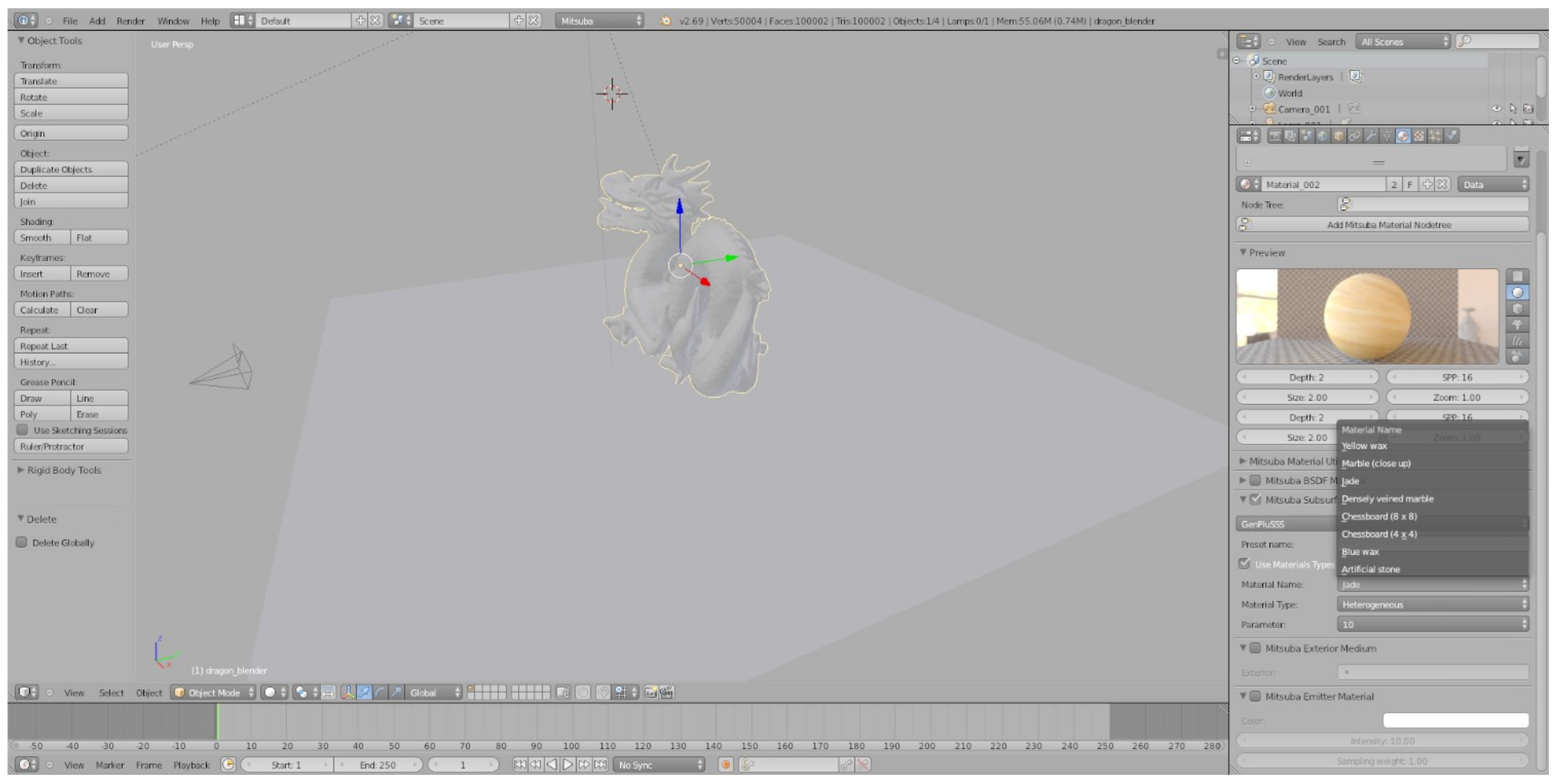
In this study, we use genetic optimization and an SVD-based subsurface scattering approach (GenSSS) for compact and accurate representation of heterogeneous, optically thick, translucent materials. The GenSSS method combines GA-based optimization and SVD-based representation [3]. This approach was implemented in the Mitsuba renderer [4] and was included as an integrated plugin in the Blender 3D modeling tool [5]. Our plugin (GenPluSSS) integrates this method into an accessible, production-oriented rendering workflow and supports both homogeneous and heterogeneous material types. As illustrated in Figure 1, heterogeneous subsurface scattering effects can be demonstrated visually and plausibly using the proposed plugin.
Despite these advances, measured subsurface scattering methods have remained largely confined to standalone research implementations, with limited integration into artist-oriented 3D production environments. Practitioners working in visual effects, game development, and architectural visualization typically rely on analytical approximations—such as the dipole model—because data-driven methods offer no accessible tooling within standard content creation pipelines. This disconnect means that the accuracy gains offered by measured BSSRDF data are rarely exploited in practice. GenPluSSS addresses this gap directly: by packaging the GenSSS representation as a Blender plugin, it enables artists and researchers to render optically thick translucent materials from measured data without leaving a familiar open-source environment, while the K parameter allows render time to be traded against visual fidelity—a practical concern wherever render budgets are fixed.
Although GenSSS was previously introduced as a standalone representation method, this work integrates it into a Blender–Mitsuba rendering workflow and provides validation on measured datasets with comparative analysis.
In summary, the main contributions of this paper are:
- A unified Blender-based rendering workflow for representing both homogeneous and heterogeneous optically thick translucent materials within a practical artist-oriented interface.
- A tuneable plugin to trade visual complexity against rendering times through the K parameter.
- A detailed validation of GenPluSSS on measured subsurface scattering datasets, including rendering times and peak memory usage.
- A comparison to the state-of-the-art, showing significant improvements in terms of rendering times of homogeneous translucent materials, including dipole-based, SVD-based, and neural subsurface scattering approaches.
Figure 1.
Overview of the Blender 3D Modeling Tool [5] with the GenPluSSS plugin. The heterogeneous Jade material is shown with .
2. Related Work
Our proposed plugin is based on Kurt’s [3] GenSSS model, which builds upon compression based representations, GAs, and BSSRDF representations. The proposed plugin is also related to prior work on compression-based scattering models and genetic algorithm-based optimization techniques. Our work is also related to plugins for BSSRDF representations, so we briefly review each of these below.
2.1. BSSRDF Representations
Jensen et al. [6] presented the diffusion dipole approximation for homogeneous subsurface scattering representation. This approach is effective for representing homogeneous translucent materials, but cannot accurately represent heterogeneous media. Jensen and Buhler [7] suggested a two-step hierarchical algorithm to calculate the dipole diffusion approximation. This algorithm is faster than Jensen et al.’s [6] BSSRDF approximation. d’Eon et al. [8] suggested a multi-layered subsurface scattering representation for real-time rendering of human skin. Jimenez et al. [9] extended Jensen et al.’s BSSRDF approximation to represent human skin in real time. To represent human skin, the diffusion dipole approximation was extended by the diffusion multipole approximation, which was proposed by Donner and Jensen [10]. Jakob et al. [11] extended Jensen et al.’s BSSRDF approximation by using an anisotropic approach. Yatagawa et al. [12] suggested a real-time screen-space rendering technique for representing the heterogeneity of subsurface scattering. The proposed technique is referred to as LinSSS. However, their goal is not to represent smaller approximation errors, but to provide an approximation that can be used in real-time screen-space rendering, prioritizing runtime performance over approximation accuracy. Recently, TG et al. [13,14] proposed Neural SSS and Neural BSSRDF, which enables more efficient and accurate rendering of heterogeneous translucent objects through the adoption of lightweight neural networks. This work represents a significant step toward applying learned function approximation to physically based subsurface scattering rendering. However, these neural approaches typically rely on GPU inference and are mainly designed for heterogeneous scattering representations. In addition, they may not accurately represent homogeneous translucent materials. In contrast, GenPluSSS supports both homogeneous and heterogeneous translucent materials within the Blender ecosystem.
2.2. Compression-Based Representations
In computer graphics, factorization-based representations have been used for representing BRDFs [15,16], BTFs [17,18], homogeneous subsurface scattering [19], and heterogeneous subsurface scattering [20,21]. These factorization-based methods have been widely applied for compact and efficient scattering representations. Yatagawa et al. [22] suggested a data compression method for measured heterogeneous subsurface scattering since the large data sizes cause problems for devices, which have limited memory, such as tablets and mobile phones, in real-time rendering, targeting memory-constrained devices.
2.3. Genetic Algorithms
Genetic algorithms are less applied to problems in computer graphics and have been used extensively in optimization problems [3]. Kurt [3] used GA and reported that when compared to inverse-rendering-based techniques [23,24], his GA is computationally efficient as his fitness function is computed between measured and factored data for each candidate chromosome. The range parameter identified by the GA, combined with SVD factorization, forms the core of the GenSSS method that underlies GenPluSSS.
2.4. Plugins for BSSRDF Representations
Blender 3D modeling tool [5] includes a plugin for the diffusion dipole approximation, which is used to represent optically thick, homogeneous translucent materials. Styperek and Juhé [25] proposed the plugin, which was developed by using the Mitsuba renderer [4]. Önel et al. [26] proposed a plugin for representing optically thick, homogeneous translucent materials. The proposed plugin is based on an SVD approach proposed by Kurt [21]. Similar to Styperek and Juhé [25], Önel et al. [26] prepared the plugin for the Blender 3D modeling tool by using the Mitsuba renderer [4].
OpenPBR surface model [27] is open-source, designed as an über-shader. It aims to be capable of accurately modeling the vast majority of CG materials used in practical visual effects and feature animation productions. The OpenPBR has been developed as a synthesis of the Autodesk Standard Surface and the Adobe Standard Material models. OpenPBR includes a plugin for the diffusion dipole approximation [6], which is used to represent optically thick, homogeneous translucent materials. Recently, NVIDIA presented open-source RTX Character Rendering (RTXCR) [28], which implements techniques used to render realistic human hair and skin. RTXCR introduces a novel hair data structure called Linear-Swept Sphere (LSS). For skin, RTXCR implements a combined subsurface scattering solution that extends the SOTA Burley Diffusion Profile with a single scattering term. This provides better support for both backward scattering from diffusion profile and forward transmission from single scattering [28].
Unlike previous works, Kurt’s GA [3] combined with the SVD-based technique provides a new approach to representing measured subsurface scattering data of translucent materials. This was the main motivation for our work. Our work extends this line of development by integrating GA-based optimization into the plugin pipeline, enabling more accurate and compact representations for both homogeneous and heterogeneous material classes. Thus, homogeneous and heterogeneous subsurface scattering representations have become available for the Blender 3D modeling tool.
3. Our Integration Plugin (GenPluSSS)
In this work, our goal is to develop a plugin for rendering optically thick, translucent materials. The proposed plugin can be considered as an interface between the renderer and the 3D modeling tool. The properties of lighting, shading, and texture mapping in the scene are defined by the 3D modeling tool. Then, to get the final image, the scene configuration is sent to the renderer. Light sources, materials and their properties can be easily configured using the 3D modeling tool.
Blender [5] is an open-source development platform. Blender uses Python 2.7 [29] as its scripting language and provides an interface to C++ functionalities through bindings and APIs, enabling interoperability with C++-based rendering systems. Since Mitsuba [4] is an open-source renderer written in C++, we selected Blender and Mitsuba for the implementation of GenPluSSS.
Other advantages of selecting Mitsuba as an open-source renderer include performance, scalability, robustness, physical accuracy, and ease of use. The proposed plugin was implemented in the Python programming language, so interaction between GenPluSSS and Mitsuba is simplified through a Python-based interface layer.
In this study, to make a fair comparison with existing plugins, we used Mitsuba version 0.5.0 and Blender version 2.69. A general overview of the Blender 3D modeling tool and our integration plugin (GenPluSSS) can be seen in Figure 1.
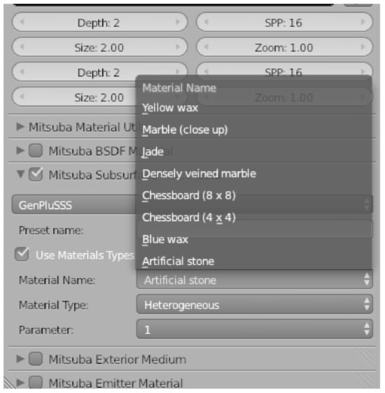
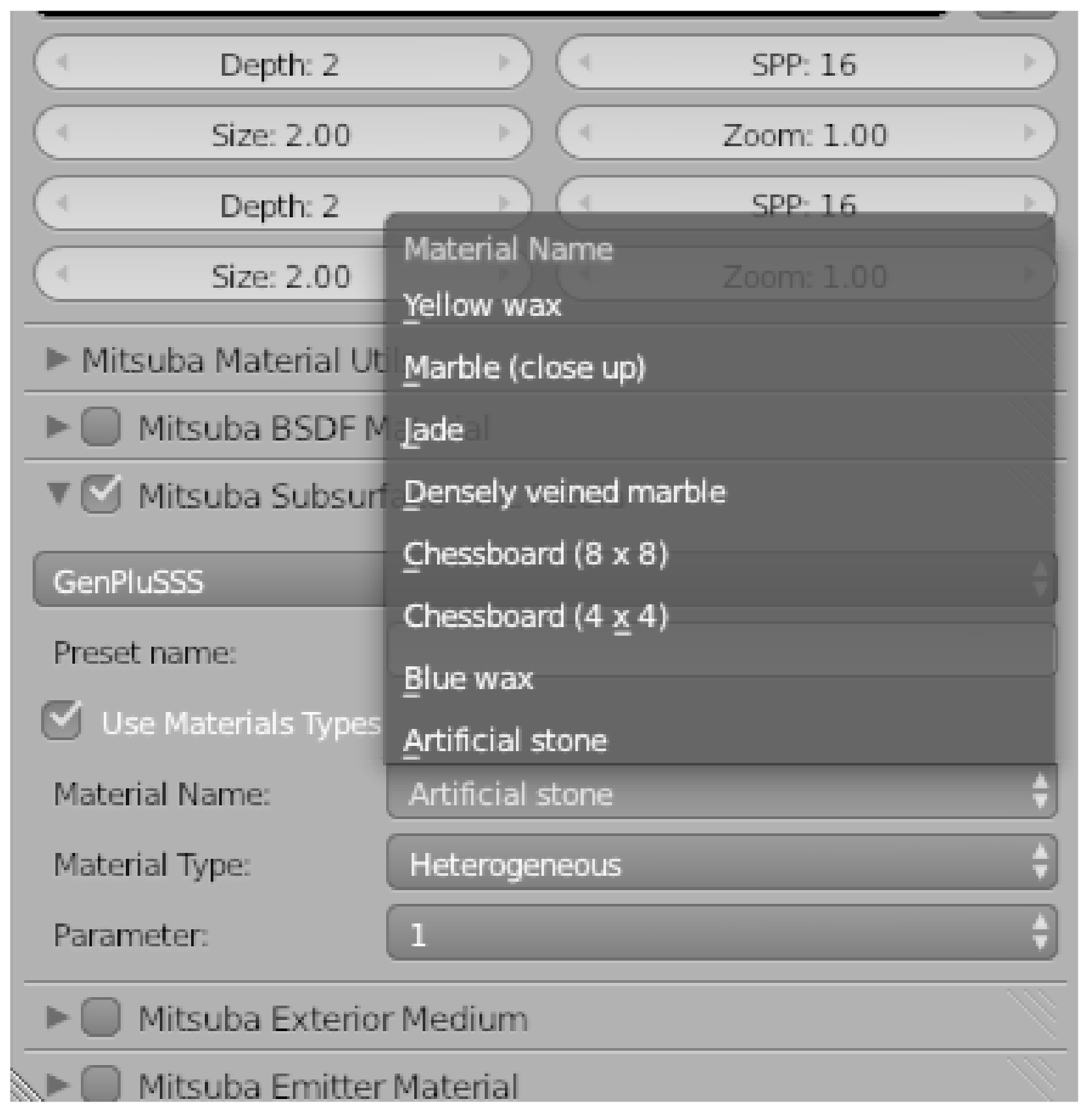
The GUI (Figure 2) provides three controls: material name, material type, and the K parameter. Material names include “Artificial stone”, “Blue wax”, “Chessboard ()”, “Chessboard ()”, “Densely veined marble”, “Jade”, “Marble (close up)”, and “Yellow wax”, drawn from the measured datasets of Peers et al. [20] and Song et al. [30] (see Figure 2). Either “Homogeneous” or “Heterogeneous” material type can be selected. If the material type is selected as heterogeneous, the value of the K parameter—labeled “Parameter” in the plugin—can be set to “1”, “5”, or “10”. For homogeneous materials, the K parameter control is hidden and the default value of 1 is used.
Figure 2.
The graphical user interface of the GenPluSSS plugin in the Blender 3D Modeling Tool [5], showing material name, type, and K parameter controls.
The GenSSS model uses an error modeling approach [31] using SVD-based factorization to represent the measured subsurface scattering matrix . First, the BSSRDF matrix is reformatted by aligning the diagonal by a change of variables () to , similar to [20]. Second, various transformation operations are applied to obtain the subsurface scattering matrix using a genetic algorithm. In this process, the fitness (i.e., loss function) of a chromosome is defined as the Root-Mean-Square Error (RMSE) between measured and factored subsurface scattering data. To reconstruct from , it is necessary to store the fittest parameters (i.e., the fittest chromosome) of the applied transformations. The final subsurface scattering model will be the sum of the estimation of model errors and the first factorization of , which can be formalized as:
where and are incoming and outgoing surface locations, , K is the total number of terms, and are the univariate functions, which help to provide a very compact subsurface scattering representation. In GenPluSSS, K provides some controllability of the modeling errors of the GenSSS model. The K parameter provides control over the visual quality of GenPluSSS. It also affects the rendering times of GenPluSSS linearly.
GenSSS representation has four parameters: , , and K. The parameter is computed from the measured subsurface scattering profiles. and are both scalar values and are determined using a genetic algorithm. K is the number of terms in the SVD-based factorization used in the GenSSS model. Minimizing K in GenSSS plays a key role when lower rendering times are desirable. Another important parameter is the range, which defines the interval over which the transformation is applied to the subsurface scattering profiles. The genetic algorithm helps to find the optimum range of applied transformations, which also optimizes the rendering times of the GenSSS model and GenPluSSS.
To construct homogeneous BSSRDF data that exhibit radially symmetric behavior (locally homogeneous), the reparameterized matrix is used and the following computation is applied, similar to Peers et al. [20]:
where is an average response function. is an approximation of the homogeneous BSSRDF data. Therefore, can be used to create homogeneous BSSRDF data . After computing homogeneous BSSRDF data from , the same reparameterization in Equation (1) is used to compute . The computation in Equation (2) is essentially a radial averaging of the BSSRDF profiles. After constructing homogeneous BSSRDF data using Equation (2), it is represented with a rank-1 approximation of SVD. The homogeneous subsurface scattering representation of GenPluSSS provides an almost ideal representation ( for all materials) as in Equation (1) is mostly equal to in Equation (2). GenPluSSS representation is easy to compute () and provides a very compact solution, since we simply store for each color channel separately. A quantitative analysis of the effect of K on image fidelity and memory consumption is provided in Section 4.6, with supporting renderings and difference maps.
The GUI of the proposed integration plugin is shown in Figure 2. The representation of homogeneous and heterogeneous translucent materials is classified in the Mitsuba Subsurface Scattering section, which is readily available in the Mitsuba integration plugin [25]. The details of material type are chosen using the GUI (see Figure 1 and Figure 2). Since Blender [5] supports modeling different types of materials and other scene details, the selected settings take effect after the rendering step.
4. Experimental Results
The proposed plugin was validated on various translucent materials measured by Peers et al. [20] and Song et al. [30]. Subsurface scattering measurements were first modeled using the GenSSS representation [3], and the resulting parameters were loaded into the plugin for rendering. As shown in Figure 3, Figure 4, Figure 5 and Figure 6, the plugin produces homogeneous and heterogeneous subsurface scattering effects that are visually plausible, faithfully reproducing the results reported in Kurt [3]. We evaluate two practical metrics: rendering time and peak memory usage.
The materials were applied to a dragon object and a statue object to verify whether the plugin produces visually consistent subsurface scattering effects under different geometric configurations. The plugin exposes “Material Type”, “Material Name”, and “Parameter” controls (see Figure 1 and Figure 2), and the scene details were exported to the renderer successfully.
4.1. Experimental Setup
All experiments were conducted using Mitsuba renderer version 0.5.0 and Blender version 2.69. These versions were selected to ensure a fair and direct comparison with the existing dipole-based plugin [25] and the SVD-based plugin [26], both of which were developed under the same software environment.
Two scene configurations were used in this work. The full set of rendering parameters for both scene configurations is summarized in Table 1. For rendering time and peak memory benchmarks (Table 2 and Table 3), a manually constructed dragon scene was used consistently across the dipole, SVD, and GenPluSSS plugin comparisons. For image quality evaluation, two standardized scenes were used: a dragon scene and a statue scene, placed on a diffuse plane under identical spot lighting and camera configurations. The dragon mesh consists of approximately 100,000 faces and 50,000 vertices, and the statue mesh consists of approximately 483,226 faces and 241,607 vertices. Rendering time and peak memory benchmarks (Table 2 and Table 3) were measured exclusively on the manual scene; image quality metrics (PSNR, RMSE) were obtained from the standardized scenes.
Table 1.
Rendering parameters used for the manually constructed dragon scene (used for rendering time and peak memory benchmarks) and the standardized scenes (used for image quality evaluation).
Table 2.
Rendering times and peak memory usage for all materials using GenPluSSS, measured on the manually constructed dragon scene (direct illumination integrator, pixels). These figures capture only the material data and scene geometry footprint under that specific scene configuration, and are therefore not directly comparable to the memory values in Table 4, which were obtained from the standardized dragon scene using a path tracer with irradiance caching at pixels.
Table 3.
Comparison of average rendering time and peak memory usage across plugins.
Rendering time and peak memory measurements were performed on a system equipped with an Intel Core i5-3210M processor, 6 GB of RAM, and an NVIDIA GeForce GT 630M GPU. Reference images for PSNR and RMSE computation were obtained from the experimental dataset of Kurt [3], rendered using a Monte Carlo path tracing algorithm at 16 samples/pixel under the same scene configurations. Although the experimental hardware (Intel Core i5-3210M, 6 GB RAM, NVIDIA GeForce GT 630M) predates current workstation standards, the primary goal of this evaluation is a controlled, like-for-like comparison with the dipole-based plugin [25] and the SVD-based plugin [26], both benchmarked under identical hardware and software conditions. Since all three plugins are CPU-bound single-threaded renderers running under Mitsuba 0.5.0, the reported rendering times scale proportionally with CPU clock speed and core count; the relative performance ordering among the three methods is therefore hardware-independent and expected to hold on modern architectures. Absolute timing benchmarks on modern hardware are planned as part of the Blender migration described in Section 6.
Each scene was rendered once under its respective configurations as summarized in Table 1; rendering time was recorded as the wall-clock time reported by Mitsuba at the end of each render. No multiple runs were performed as the deterministic low-discrepancy sampler produces identical results across runs under fixed settings.
It should be noted that the peak memory values reported throughout this work reflect the renderer’s in-process RAM usage at render time, as logged by Mitsuba at the end of each render. This figure captures the memory footprint of the loaded scene geometry, material data, and irradiance cache during active rendering. The scene export step—in which Blender serialises the scene configuration and material parameters to disk prior to launching the renderer—involves only lightweight file I/O and does not contribute meaningfully to peak RAM consumption. Consequently, scene export overhead is not separately reported as it falls below the resolution of the renderer’s memory reporting mechanism.
4.2. Visual Results
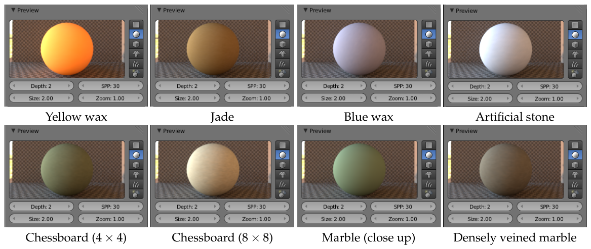
Figure 3 illustrates the sphere previews of homogeneous subsurface scattering effects, and Figure 4 illustrates the sphere previews of heterogeneous subsurface scattering effects. Both configurations include six materials evaluated quantitatively: yellow wax, jade, blue wax, artificial stone, chessboard (), and chessboard (). The sphere previews in Figure 3 and Figure 4 additionally show marble (close up) and densely veined marble for visual reference. In the preview scene in Figure 4, .
Figure 3.
Sphere previews for all eight homogeneous translucent materials rendered with GenPluSSS ().
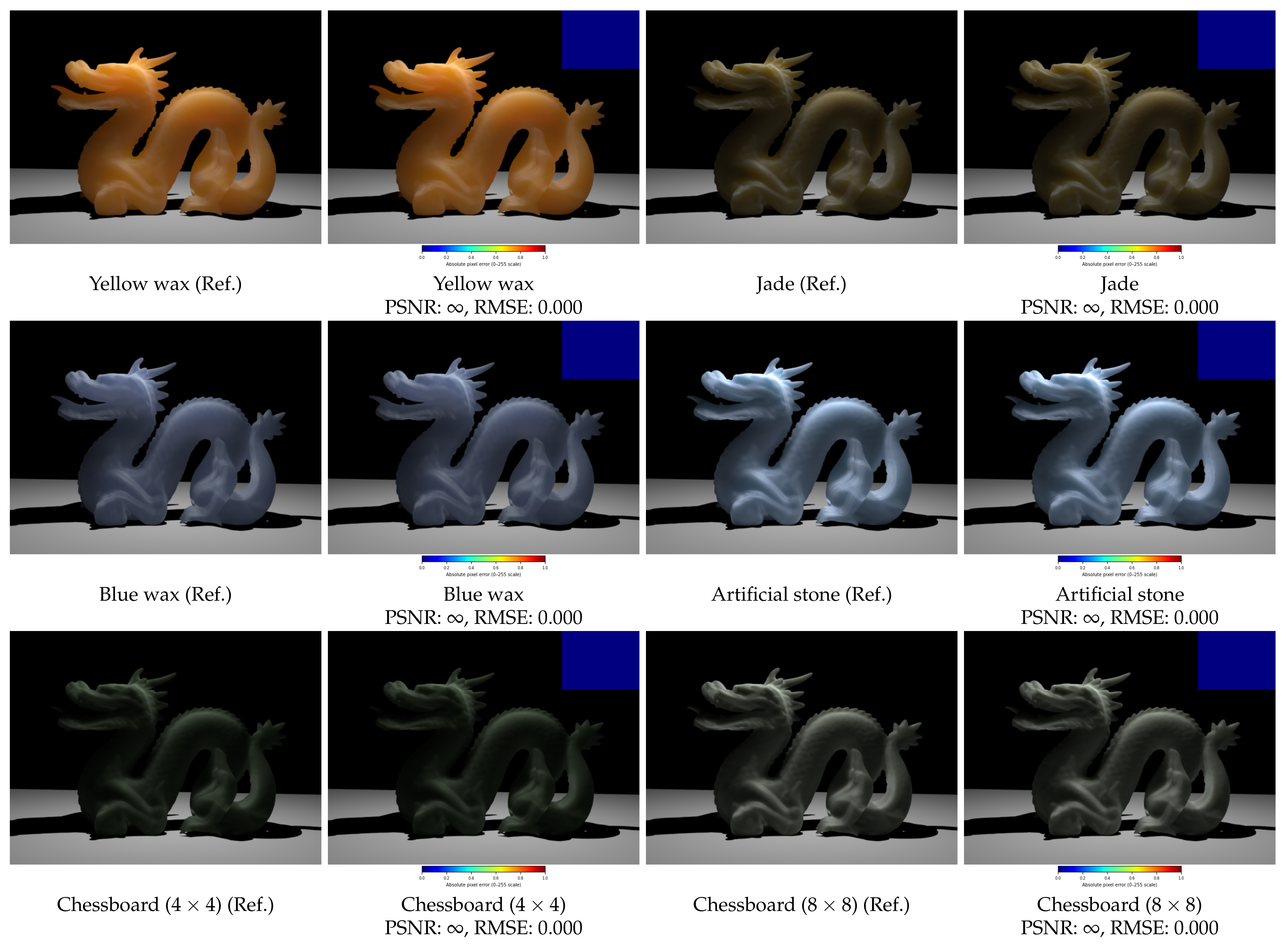
As shown in Figure 5 and Figure 6, GenPluSSS correctly renders heterogeneous and homogeneous translucent materials under the experimental conditions described in Section 4.1. Heterogeneous materials exhibit visible spatial variation in light transport—for example, the grid structure in the chessboard materials—confirming that the factored heterogeneous model is correctly applied. Homogeneous materials display spatially uniform, smooth scattering consistent with the single-basis representation.
For homogeneous materials, GenPluSSS yields PSNR and RMSE across all six tested materials. This result reflects mathematical internal consistency: the homogeneous BSSRDF data is constructed by radially averaging the measured profiles Equation (2), and the rank-1 SVD representation then reproduces this averaged function exactly. Consequently, RMSE confirms that the plugin correctly implements the representation established analytically in Section 3, rather than constituting a claim of perfect physical accuracy against the raw measured BSSRDF data.
Figure 4.
Sphere previews for all eight heterogeneous translucent materials rendered with GenPluSSS ().
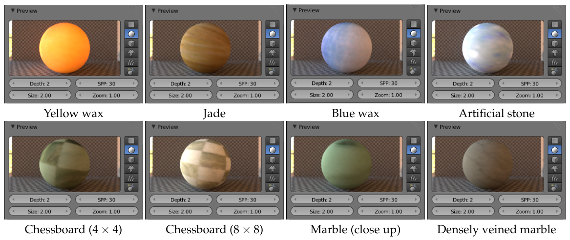
Figure 5.
Heterogeneous translucent material renderings () on a dragon object using GenPluSSS. For each material: reference image [3] (left) and GenPluSSS output with embedded difference map (right). Mean PSNR: dB. Difference maps use a JET colormap; the labeled color bar below each rendered image indicates absolute pixel error on the 0–255 intensity scale.
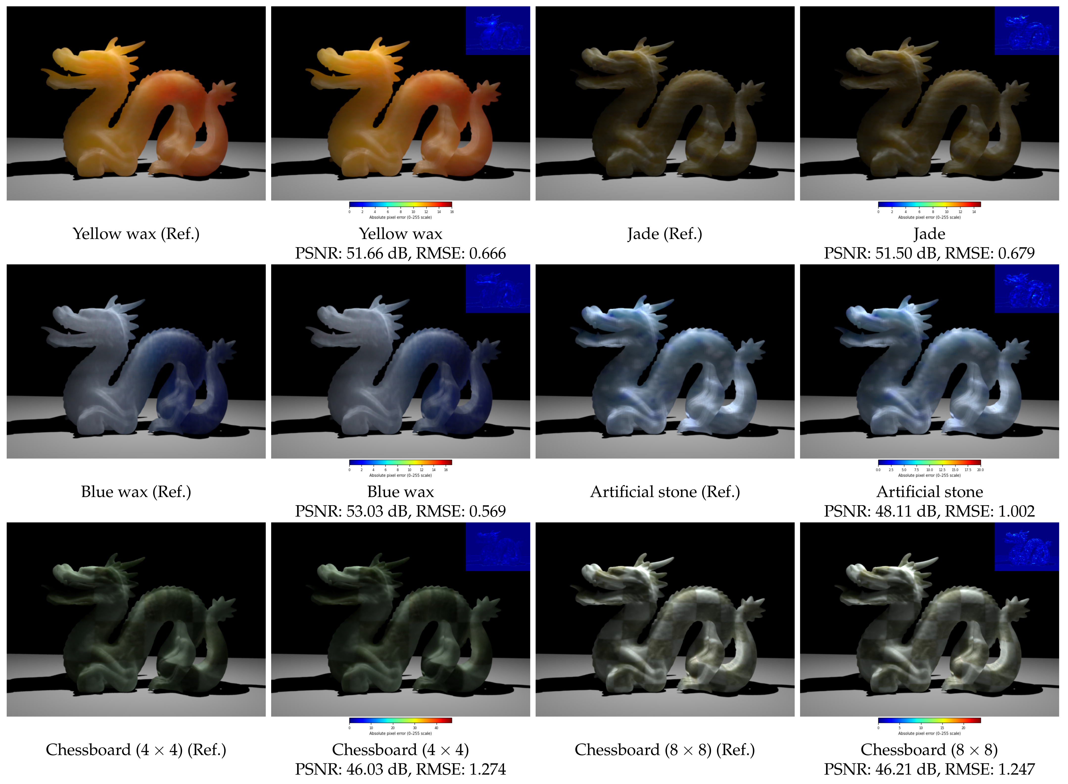
Figure 6.
Homogeneous translucent material renderings () on a dragon object using GenPluSSS. For each material: reference image [3] (left) and GenPluSSS output with embedded difference map (right). PSNR , RMSE for all materials. Difference maps use a JET colormap; the labeled color bar below each rendered image indicates absolute pixel error on the 0–255 intensity scale.
4.3. Rendering Times and Peak Memory Usage
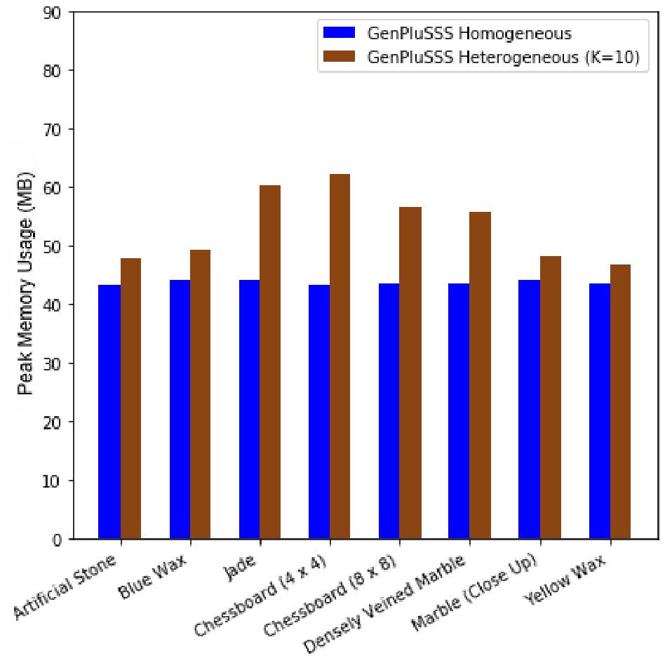
Figure 7 illustrates the rendering times of 12 homogeneous translucent materials from Jensen et al. [6], Figure 8 illustrates the rendering times of 35 homogeneous translucent materials from Narasimhan et al. [32], and Figure 9 illustrates the rendering times of homogeneous and heterogeneous translucent materials calculated with GenPluSSS. Figure 10 illustrates the peak memory usage of GenPluSSS for all homogeneous and heterogeneous translucent materials. The value of K for heterogeneous materials was 10; for homogeneous materials it was 1 (default). Higher K values increase both rendering time and peak memory usage; consequently, heterogeneous materials (K = 10) show higher values than homogeneous materials (K = 1), as seen in Figure 9 and Figure 10.
It should be noted that the peak memory values in Table 2 and Table 4 reflect different scene configurations and integrators (see Table 1), and should therefore not be compared directly. Table 2 reports memory under the manually constructed dragon scene with a direct illumination integrator, whereas Table 4 uses the standardized scene with a path tracer and irradiance caching, which introduces additional memory overhead for the irradiance cache data structure.
Table 2 summarises the per-material rendering time and peak memory results obtained from the manually constructed dragon scene. The average rendering time of homogeneous materials was 20.22 min, and the average peak memory usage was 43.70 MB. The average rendering time of heterogeneous materials was 28.88 min, and the average peak memory was 53.93 MB.
Figure 7.
Rendering times of 12 homogeneous translucent materials from Jensen et al. [6] rendered with the dipole approximation plugin [25].
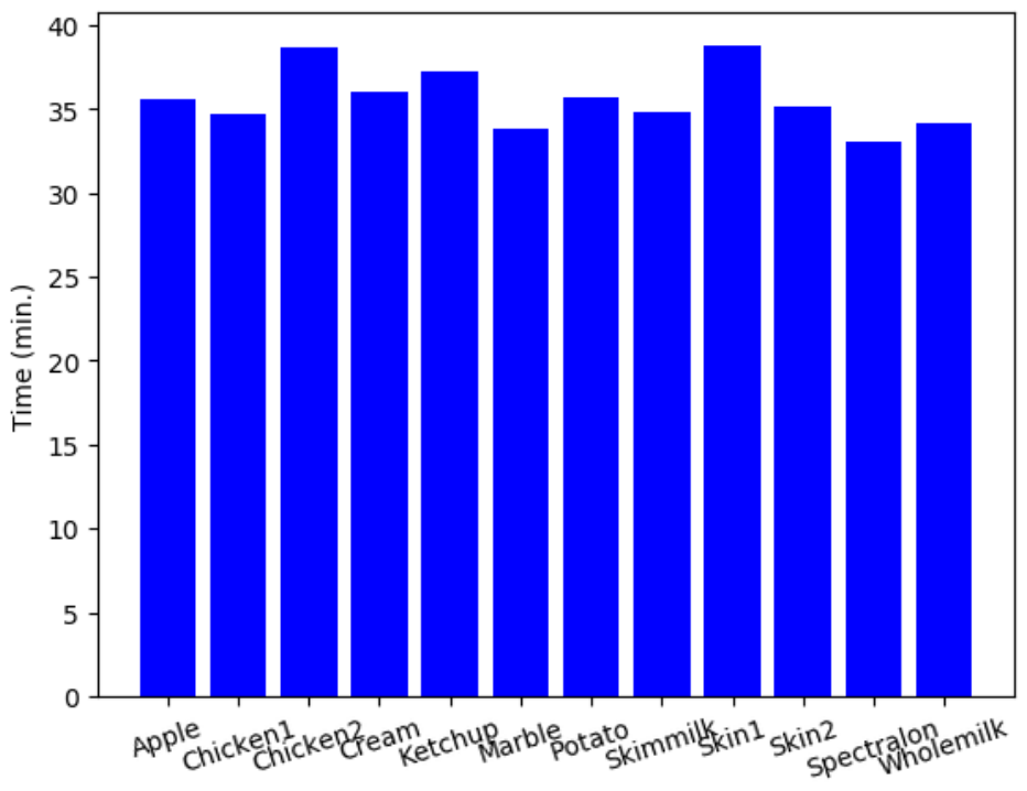
Figure 8.
Rendering times of 35 homogeneous translucent materials from Narasimhan et al. [32] rendered with the dipole approximation plugin [25].
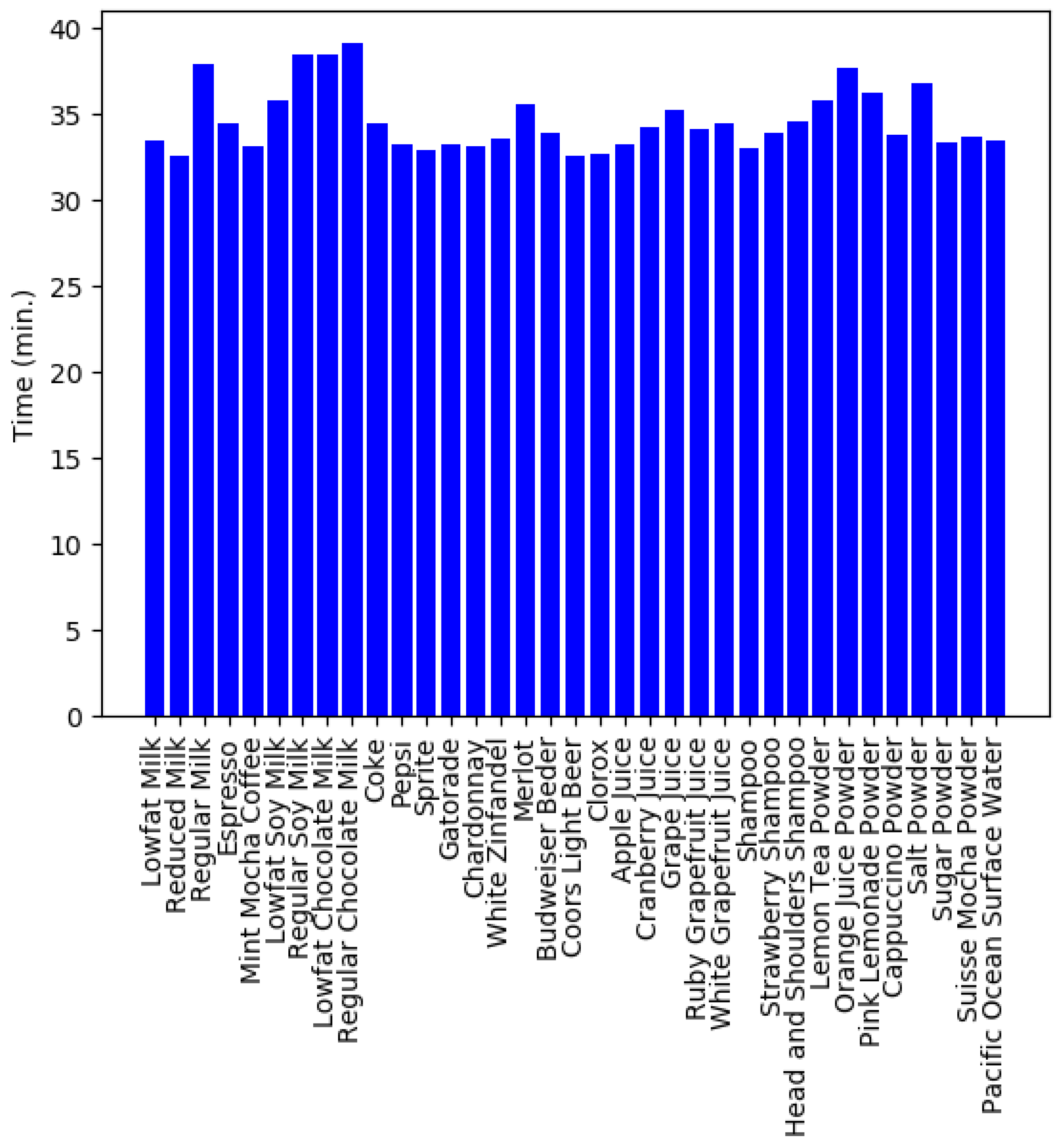
Figure 9.
Rendering time comparison for GenPluSSS across homogeneous () and heterogeneous () translucent materials.
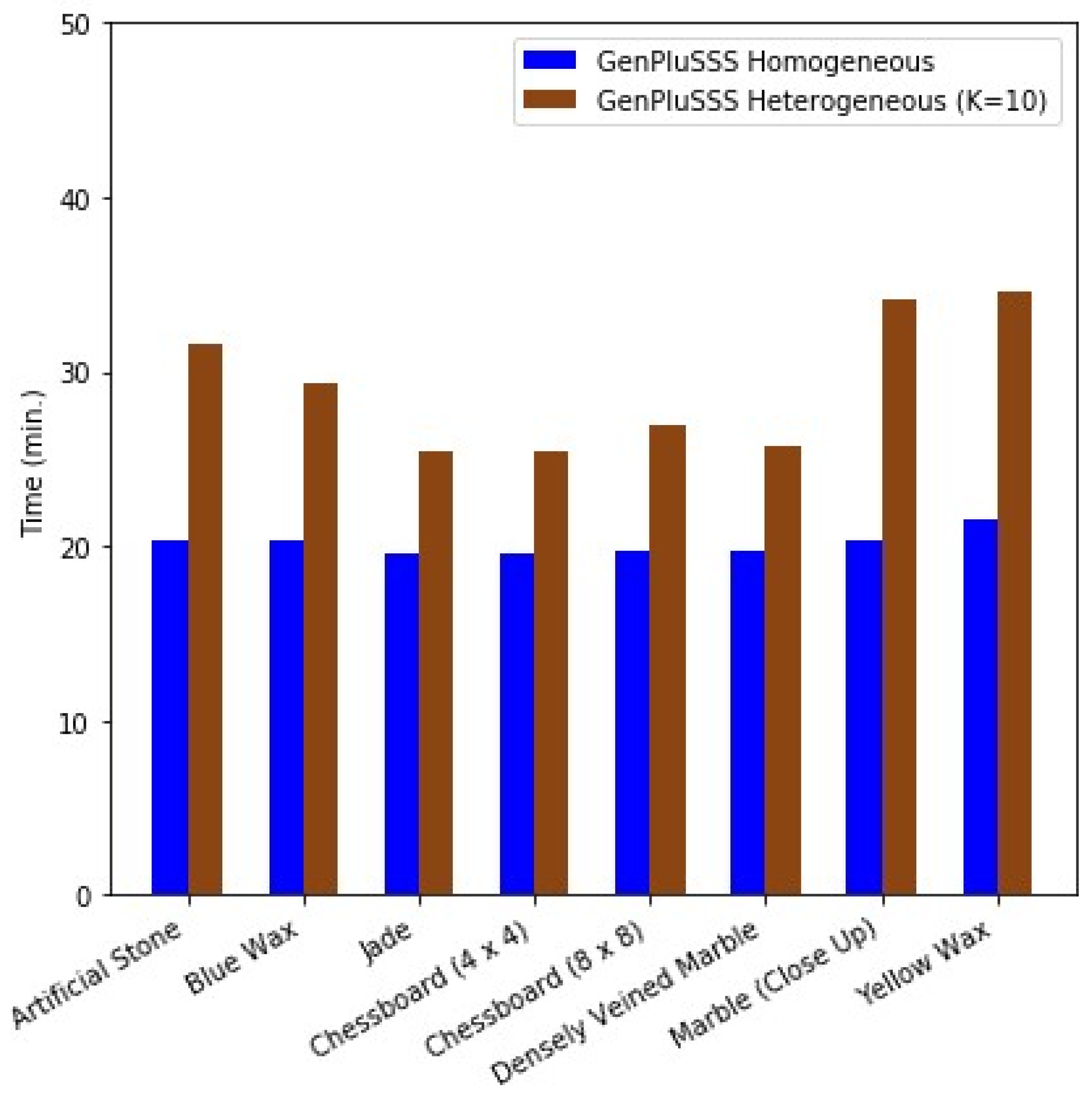
Figure 10.
Peak memory usage comparison for GenPluSSS across homogeneous () and heterogeneous () translucent materials.
4.4. Comparison with Dipole and SVD Plugins
The rendering time and peak memory comparisons in this section were obtained from the manually constructed dragon scene used consistently across the dipole, SVD, and GenPluSSS plugin benchmarks.
Using the SVD-based plugin of Önel et al. [26], the rendering time of the heterogeneous chessboard () material was 25.1 min and that of the chessboard () was 26.4 min, requiring 63.54 MB and 55.89 MB of peak memory respectively (average: 25.75 min, 59.69 MB peak memory). In GenSSS, an additional transformation step is applied on top of the SVD decomposition, which increases rendering time compared to the plain SVD method [26].
In the exporter plugin of Styperek and Juhé [25], the rendering times of 12 homogeneous translucent materials from Jensen et al. [6] with the dipole approximation were tested (see Figure 7). Samples per pixel were matched to those used by GenPluSSS to ensure a fair comparison. The average rendering time of these 12 materials was 35.6 min, whereas GenPluSSS rendered 6 homogeneous materials in an average of only 20.22 min, with an average peak memory of 43.70 MB. The 35 homogeneous materials from Narasimhan et al. [32] were also tested with the exporter plugin (see Figure 8), yielding an average rendering time of 34.6 min and an average peak memory of 43.82 MB. We acknowledge that the compared material sets are not identical across plugins: GenPluSSS was evaluated on six measured materials from Peers et al. [20] and Song et al. [30], whereas the dipole-based plugin [25] was evaluated on the Jensen et al. [6] and Narasimhan et al. [32] datasets. A direct material-matched comparison is not feasible because the dipole model operates on analytical scattering parameters rather than measured BSSRDF profiles, and the two plugin types therefore do not share a common material representation. The rendering times are nonetheless comparable as a proxy metric, since both plugins were run under the same manually constructed dragon scene with identical hardware, and the measured materials span a similar range of optical complexity. GenPluSSS is therefore considerably faster for rendering homogeneous translucent materials.
In the GenSSS model, the range parameter is as important as K for rendering time. The Genetic Algorithm finds the optimum range of applied transformations, which also reduces rendering time. Furthermore, when , the representation is computationally inexpensive. Generally, analytical subsurface scattering models consume less memory than data-driven models because data-driven representations require more data to be loaded at runtime. In our case, however, GenPluSSS also requires less peak memory than the dipole-based plugin because K is set to 1 for homogeneous materials.
Visual and Quantitative Comparison with the SVD-Based Plugin
The quantitative image quality comparison in this subsection was performed on the standardized dragon and statue scenes.
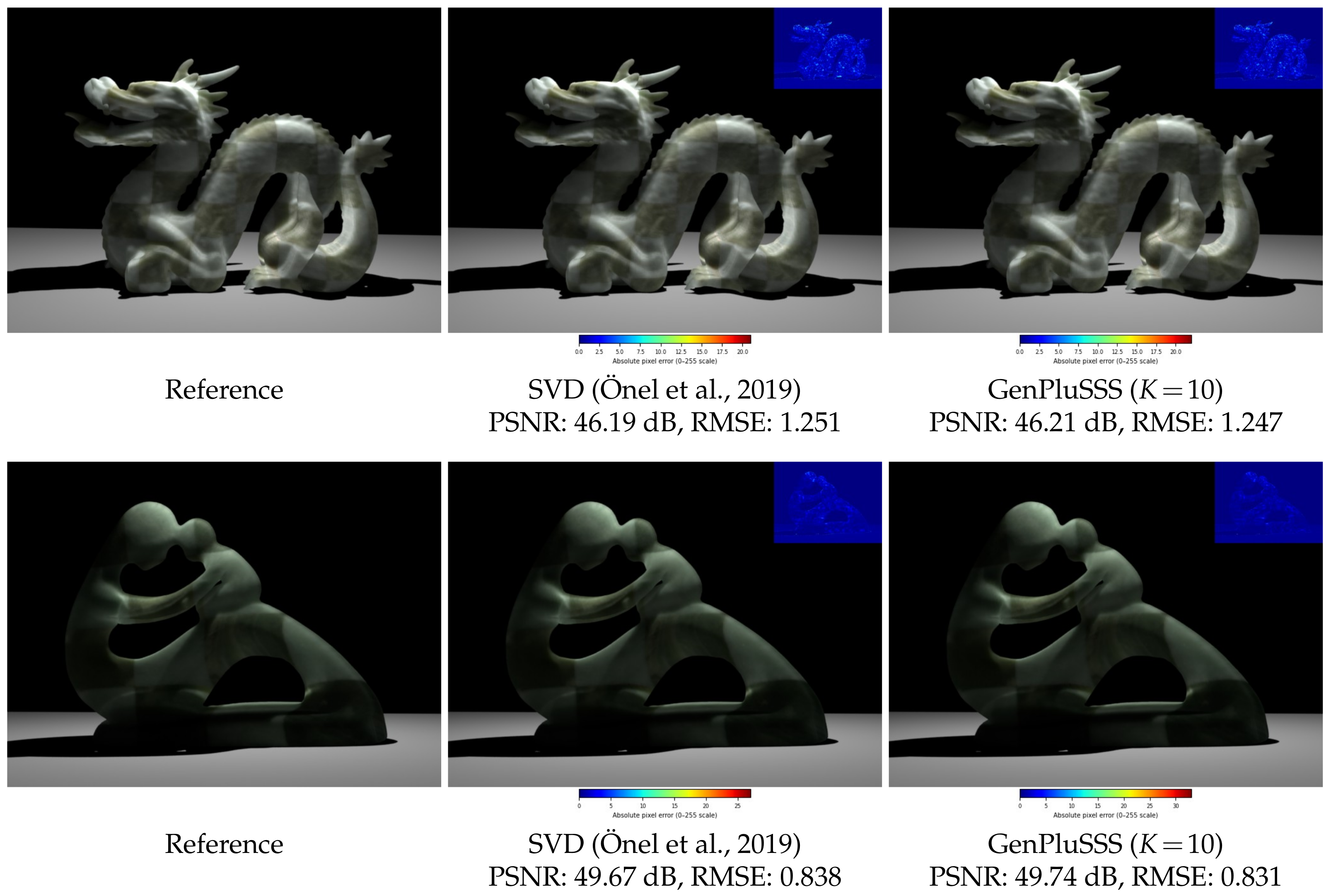
The visual plausibility of GenPluSSS renderings was assessed quantitatively by comparing rendered outputs against reference images for two heterogeneous translucent materials: Chessboard () on a dragon object and Chessboard () on a statue object. Reference images were obtained from the experimental dataset of Kurt [3], rendered using a Monte Carlo path tracing algorithm at 16 samples/pixel.
All renderings were produced under the experimental conditions described in Section 4.1.
PSNR and RMSE were computed between each method’s output and the corresponding reference image using standard full-reference image quality metrics [33]. PSNR was used to evaluate image fidelity relative to the reference render, while RMSE quantified the average pixel-wise reconstruction error.
PSNR values are reported in decibels (dB), whereas RMSE values represent the root mean square pixel error computed on the standard 8-bit RGB intensity range (0–255). The results are summarized in Figure 11.
GenPluSSS with achieves image fidelity equivalent to the SVD-based plugin [26] on both test scenes, with a PSNR difference of less than 0.1 dB and virtually identical RMSE values. For the Chessboard () material, GenPluSSS () marginally outperforms the SVD plugin (49.74 dB vs. 49.67 dB), indicating that the additional GA-based transformation stage introduces no perceptible degradation in image quality.
Figure 11 shows the rendered images with embedded difference maps (inset, upper right) for each method and scene. Difference maps were computed as the absolute per-pixel error between each output and the reference image, normalized and visualized using a JET colormap. The predominantly dark blue appearance of all difference maps confirms that pixel-level errors are perceptually negligible across both scenes and methods.
Figure 11.
Rendered results for the dragon with Chessboard () (top row) and the statue with Chessboard () (bottom row). Each image includes an embedded difference map (inset, upper right) computed against the reference image [3]. The SVD-based results correspond to the plugin by Önel et al. [26]. Difference maps are visualized using a JET colormap scaled to the per-image maximum absolute pixel error, where dark blue indicates near-zero error and warm colors (yellow–red) indicate larger deviations; the numerical scale is provided in the color bar below each rendered image.
4.5. Comparison with Recent Neural SSS Methods
Neural approaches such as Neural SSS [14] and Neural BSSRDF [13] represent significant advancements in subsurface scattering research, achieving high-fidelity representations of heterogeneous translucent objects through lightweight neural networks. Table 5 provides a structured comparison of GenPluSSS with these and other recent methods in terms of approach type and material support. Mean PSNR values, where available, are discussed in the text below rather than tabulated, since the methods were evaluated on different scenes and datasets, making direct numerical comparison misleading.
The mean PSNR of 49.42 dB reported for GenPluSSS is the arithmetic mean of PSNR values computed across all rendered heterogeneous translucent materials () in our experimental evaluation. For homogeneous materials, RMSE = 0 across all tested materials, yielding PSNR ; this result reflects an exact representation.
For TG et al. [13], PSNR is not reported directly in that work; the PSNR value is derived from the per-scene MSE values given in Table 1 of that paper using the standard PSNR definition [33]:
In Equation (3), is for normalized images. The mean is taken as the arithmetic mean of per-scene PSNR values, yielding 36.92 dB.
For TG et al. [14], per-pixel MSE values are not reported; that work relies solely on the FLIP perceptual difference metric, reporting a mean FLIP of 0.017 across its comparison scenes. Since no MSE values are available, a PSNR equivalent cannot be derived.
As shown in Table 5, none of the listed neural approaches supports both homogeneous and heterogeneous materials, and none provides integration with a 3D modeling tool such as Blender. GenPluSSS supports both homogeneous and heterogeneous translucent materials and runs on a CPU within the open-source Blender environment.
The comparison is therefore intended as a high-level contextual overview rather than a strict benchmark.
4.6. Effect of the K Parameter on Image Quality and Memory Usage
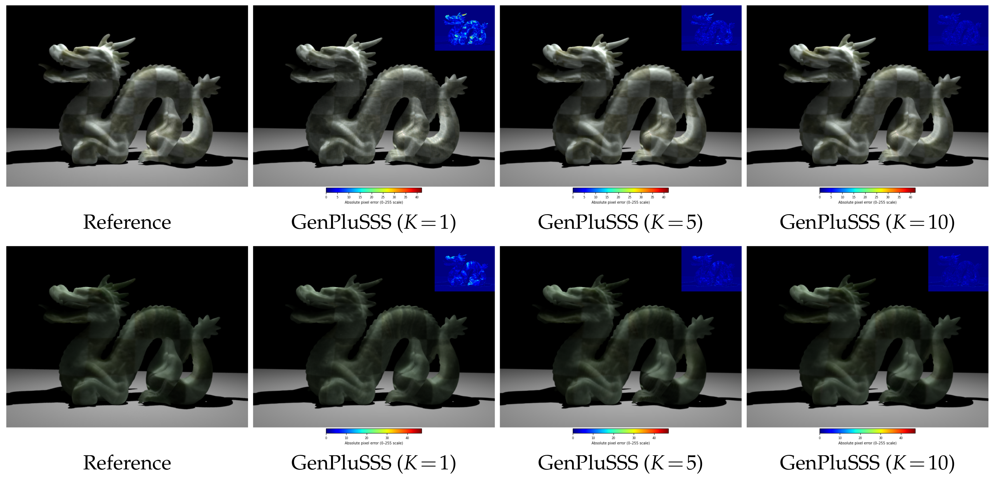
To quantify the effect of the K parameter on visual fidelity and memory consumption, the dragon object was rendered with Chessboard () and Chessboard () materials at three factorization ranks: , , and . PSNR and RMSE were computed against the reference images from Kurt [3] using standard full-reference image quality metrics [33]. Peak memory consumption during rendering was also recorded. The results are presented in Table 4 and Figure 12.
Table 4.
Effect of the K parameter on image quality and memory usage for Chessboard () and Chessboard () materials rendered on the standardized dragon scene.
Table 5.
Comparison with recent SSS representations.
As shown in Table 4 and Figure 12, increasing K yields a consistent and substantial improvement in image fidelity across both materials. At , PSNR reaches 44.14 dB and 43.30 dB for Chessboard () and Chessboard () respectively, representing a significant gain over while requiring only modest additional memory. At , PSNR further increases to 46.03 dB and 46.21 dB—an overall improvement of approximately 7.7 dB and 10.6 dB over —while RMSE decreases by more than a factor of two in both cases. Among the tested configurations, emerges as a balanced choice: it captures most of the quality improvement associated with while incurring a lower computational overhead, making it suitable for applications where rendering efficiency is a priority. The difference maps in Figure 12 further illustrate this trend: at , warmer colors are visible across the object surface, indicating non-negligible reconstruction error, whereas at the maps are predominantly dark blue, confirming perceptually negligible differences from the reference. The corresponding increase in peak memory consumption is modest, ranging from 183.3 MB to 200.2 MB for Chessboard () and from 183.0 MB to 193.0 MB for Chessboard ()—an increase of approximately 9% and 5%, respectively. These results confirm that higher K values deliver substantially improved visual quality at a relatively small memory overhead.
Figure 12.
Effect of the K parameter on rendered image quality for Chessboard () (top row) and Chessboard () (bottom row) on a dragon object. Each rendered image includes an embedded difference map (inset, upper right) computed against the reference image [3]. Difference maps use a JET colormap with a labeled color bar indicating absolute pixel error on the 0–255 intensity scale.
Based on the quantitative results in Table 4, the following practical guidelines are proposed for selecting K. For applications where rendering time is the primary constraint—such as interactive previsualization or animation batch rendering— is recommended for homogeneous materials, as it yields exact representation (RMSE = 0) at minimal computational cost. For heterogeneous materials under time-sensitive conditions, provides a balanced trade-off, recovering approximately 75% of the quality gain of (PSNR improvement of ∼5–8 dB over ) while maintaining lower rendering overhead. When visual fidelity is paramount—for example, in final-frame production rendering or scientific visualization— is recommended as it delivers the highest reconstruction accuracy with only a 5–9% increase in peak memory relative to . In general, materials with more complex spatial heterogeneity (e.g., densely patterned structures such as the chessboard materials) benefit most from higher K values.
5. Conclusions
In this paper, we presented our integration plugin (GenPluSSS) for rendering homogeneous and heterogeneous optically thick translucent materials. GenPluSSS is based on the GenSSS model, which was proposed by Kurt [3], and this plugin enables visually plausible subsurface scattering synthesis within a Blender-native rendering workflow. Sphere previews of both homogeneous and heterogeneous materials were demonstrated within the Blender interface using measured datasets. Furthermore, we made comparisons between GenPluSSS and the other integration plugins [25,26] for the average rendering times and the average peak memory usage.
Experimental comparisons with existing integration plugins showed that GenPluSSS achieves efficient rendering performance for homogeneous translucent materials while maintaining accurate visual representation quality. The proposed plugin uses GA-based optimization and SVD factorization to produce compact BSSRDF representations for both homogeneous and heterogeneous materials.
GenPluSSS achieves substantially shorter rendering times for homogeneous translucent materials. Experimental results on six measured materials demonstrated that GenPluSSS achieves an average rendering time of 20.22 min for homogeneous materials, corresponding to an improvement of approximately 43% compared to the dipole-based plugin [25]. For heterogeneous materials, GenPluSSS achieved an average peak memory reduction of approximately 9% compared to the SVD-based approach [26] while introducing a moderate increase in rendering time due to the additional GA-based transformation stage.
Quantitative evaluation against reference renderings from Kurt [3] demonstrated that GenPluSSS achieves an exact representation for all homogeneous materials (RMSE = 0, PSNR ) and image fidelity equivalent to the SVD-based plugin [26] for heterogeneous materials with , with a PSNR difference of less than 0.1 dB on both test scenes. A systematic analysis of the K parameter further confirmed that increasing K from 1 to 10 yields a substantial improvement in PSNR of up to 10.6 dB, while peak memory consumption increases by only 5–9%, providing users with a practical and well-characterized trade-off between visual quality and computational cost.
The results also demonstrate that GenPluSSS can accurately represent subsurface scattering effects in both homogeneous and heterogeneous translucent materials. Finally, comparisons with recent neural subsurface scattering methods [13,14,34,35] show that GenPluSSS renders both homogeneous and heterogeneous translucent materials on CPUs within the open-source Blender environment.
6. Future Works
We acknowledge that Blender 2.69 and Mitsuba 0.5.0 represent legacy software versions that predate current production pipelines. These versions were retained to enable a direct, controlled comparison with existing plugins [25,26] developed under the same environment. The practical implication is that GenPluSSS, in its current form, is not immediately deployable in modern Blender () and Mitsuba 2/3 workflows; migration to current versions is identified as a priority for future work.
Our GenPluSSS works in texture space. GenPluSSS assumes simplified, flat half-spaces and static geometries. By integrating dense correspondence methods, we can bridge the gap between subsurface light transport physics and dynamic, complex 3D facial morphology. Using landmark-free dense correspondence, we can map a target face precisely to a canonical, high-fidelity medical/optical face template. This allows one to accurately transfer heterogeneous material properties down to the vertex or texture level without spatial warping artifacts. This topic will be another direction for our future work.
Author Contributions
Conceptualization, B.Y. and M.K.; methodology, M.K.; software, B.Y.; validation, B.Y. and M.K.; formal analysis, B.Y. and M.K.; investigation, B.Y. and M.K.; resources, B.Y. and M.K.; data curation, B.Y.; writing—original draft preparation, B.Y.; writing—review and editing, B.Y. and M.K.; visualization, B.Y.; supervision, M.K.; project administration, M.K.; funding acquisition, M.K. All authors have read and agreed to the published version of the manuscript.
Funding
This research was funded by the Scientific and Technical Research Council of Turkey, grant number 119E092.
Data Availability Statement
To improve the transparency of our submission, we have prepared a supplementary package including interactive comparisons, the source code of the proposed algorithm, and the related datasets (including readme files). The package is publicly archived at GitHub: https://github.com/BarisYildirim10/GenPluSSS (accessed on 9 June 2026). A mirror is also available at http://akademik.ube.ege.edu.tr/~kurt/genplussswebpagecomp.zip (accessed on 9 June 2026).
Acknowledgments
The authors would like to thank the anonymous reviewers for their valuable comments. The authors would also like to thank Pieter Peers et al. [20] and Ying Song et al. [30] for sharing their measured subsurface scattering datasets.
Conflicts of Interest
Author Barış Yıldırım was employed by İzmir Innovation and Technology Inc. The remaining authors declare that the research was conducted in the absence of any commercial or financial relationships that could be construed as a potential conflict of interest.
References
- Nicodemus, F.E.; Richmond, J.C.; Hsia, J.J.; Ginsberg, I.W.; Limperis, T. Geometrical Considerations and Nomenclature for Reflectance. In Monograph, National Bureau of Standards (US); US Department of Commerce: Washington, DC, USA, 1977. [Google Scholar]
- Frisvad, J.R.; Jensen, S.A.; Madsen, J.S.; Correia, A.; Yang, L.; Gregersen, S.K.S.; Meuret, Y.; Hansen, P.E. Survey of Models for Acquiring the Optical Properties of Translucent Materials. Comput. Graph. Forum 2020, 39, 729–755. [Google Scholar] [CrossRef] [Scilit]
- Kurt, M. GenSSS: A genetic algorithm for measured subsurface scattering representation. Vis. Comput. 2021, 37, 307–323. [Google Scholar] [CrossRef] [Scilit]
- Jakob, W. Mitsuba Renderer. 2010. Available online: http://www.mitsuba-renderer.org (accessed on 9 June 2026).
- Blender. Blender Foundation. 2003. Available online: http://www.blender.org/ (accessed on 9 June 2026).
- Jensen, H.W.; Marschner, S.R.; Levoy, M.; Hanrahan, P. A practical model for subsurface light transport. In Proceedings of the 28th Annual Conference on Computer Graphics and Interactive Techniques (SIGGRAPH ’01); Association for Computing Machinery: New York, NY, USA, 2001; pp. 511–518. [Google Scholar] [CrossRef] [Scilit]
- Jensen, H.W.; Buhler, J. A rapid hierarchical rendering technique for translucent materials. ACM Trans. Graph. 2002, 21, 576–581. [Google Scholar] [CrossRef] [Scilit]
- D’Eon, E.; Luebke, D.; Enderton, E. Efficient rendering of human skin. In Proceedings of the 18th Eurographics Conference on Rendering Techniques, Grenoble, France, 25–27 June 2007; pp. 147–157. [Google Scholar]
- Jimenez, J.; Sundstedt, V.; Gutierrez, D. Screen-space perceptual rendering of human skin. ACM Trans. Appl. Percept. 2009, 6, 23:1–23:15. [Google Scholar] [CrossRef] [Scilit]
- Donner, C.; Jensen, H.W. Light diffusion in multi-layered translucent materials. ACM Trans. Graph. 2005, 24, 1032–1039. [Google Scholar] [CrossRef] [Scilit]
- Jakob, W.; Arbree, A.; Moon, J.T.; Bala, K.; Marschner, S. A Radiative Transfer Framework for Rendering Materials with Anisotropic Structure. ACM Trans. Graph. 2010, 29, 53:1–53:13. [Google Scholar] [CrossRef] [Scilit]
- Yatagawa, T.; Yamaguchi, Y.; Morishima, S. LinSSS: Linear decomposition of heterogeneous subsurface scattering for real-time screen-space rendering. Vis. Comput. 2020, 36, 1979–1992. [Google Scholar] [CrossRef] [Scilit]
- TG, T.; Frisvad, J.R.; Ramamoorthi, R.; Jensen, H.W. Neural BSSRDF: Object Appearance Representation Including Heterogeneous Subsurface Scattering. arXiv 2023, arXiv:2312.15711. [Google Scholar] [CrossRef] [Scilit]
- TG, T.; Tran, D.M.; Jensen, H.W.; Ramamoorthi, R.; Frisvad, J.R. Neural SSS: Lightweight Object Appearance Representation. Comput. Graph. Forum 2024, 43, e15158. [Google Scholar] [CrossRef] [Scilit]
- Sun, X.; Zhou, K.; Chen, Y.; Lin, S.; Shi, J.; Guo, B. Interactive relighting with dynamic BRDFs. ACM Trans. Graph. 2007, 26, 27:1–27:10. [Google Scholar] [CrossRef] [Scilit]
- Tongbuasirilai, T.; Unger, J.; Kronander, J.; Kurt, M. Compact and intuitive data-driven BRDF models. Vis. Comput. 2020, 36, 855–872. [Google Scholar] [CrossRef] [Scilit]
- Ruiters, R.; Klein, R. BTF Compression via Sparse Tensor Decomposition. Comput. Graph. Forum 2009, 28, 1181–1188. [Google Scholar] [CrossRef] [Scilit]
- Ruiters, R.; Schwartz, C.; Klein, R. Data Driven Surface Reflectance from Sparse and Irregular Samples. Comput. Graph. Forum 2012, 31, 315–324. [Google Scholar] [CrossRef] [Scilit]
- Jimenez, J.; Zsolnai, K.; Jarabo, A.; Freude, C.; Auzinger, T.; Wu, X.C.; der Pahlen, J.; Wimmer, M.; Gutierrez, D. Separable Subsurface Scattering. Comput. Graph. Forum 2015, 34, 188–197. [Google Scholar] [CrossRef] [Scilit]
- Peers, P.; vom Berge, K.; Matusik, W.; Ramamoorthi, R.; Lawrence, J.; Rusinkiewicz, S.; Dutré, P. A compact factored representation of heterogeneous subsurface scattering. ACM Trans. Graph. 2006, 25, 746–753. [Google Scholar] [CrossRef] [Scilit]
- Kurt, M.; Öztürk, A.; Peers, P. A Compact Tucker-Based Factorization Model for Heterogeneous Subsurface Scattering. In Proceedings of the 11th Theory and Practice of Computer Graphics, Bath, UK, 5–6 September 2013; Czanner, S., Tang, W., Eds.; The Eurographics Association: Eindhoven, The Netherlands, 2013; pp. 85–92. [Google Scholar] [CrossRef]
- Yatagawa, T.; Todo, H.; Yamaguchi, Y.; Morishima, S. Data compression for measured heterogeneous subsurface scattering via scattering profile blending. Vis. Comput. 2020, 36, 541–558. [Google Scholar] [CrossRef] [Scilit]
- Masia, B.; Munoz, A.; Tolosa, A.; Anson, O.; Lopez-Moreno, J.; Jimenez, J.; Gutierrez, D. Genetic algorithms for estimation of reflectance parameters. In Proceedings of the 25th Spring Conference on Computer Graphics, SCCG ’09, New York, NY, USA, 3–7 August 2009; pp. 39–44. Available online: https://api.semanticscholar.org/CorpusID:275950550 (accessed on 9 June 2026).
- Munoz, A.; Masia, B.; Tolosa, A.; Gutierrez, D. Single-image appearance acquisition using genetic algorithms. In Proceedings of the IADIS International Conference on Computer Graphics, Visualization, Computer Vision and Image Processing, IADIS ’09, Algarve, Portugal, 20–22 June 2009; pp. 24–32. Available online: https://webdiis.unizar.es/~bmasia/files/Munoz_CGVCVIP2009.pdf (accessed on 9 June 2026).
- Styperek, B.; Juhé, F. The Blender Plugin. 2011. Available online: https://www.mitsuba-renderer.org/plugins.html (accessed on 9 June 2026).
- Önel, S.; Kurt, M.; Öztürk, A. An Efficient Plugin for Representing Heterogeneous Translucent Materials. In Contemporary Topics in Computer Graphics and Games: Selected Papers from the Eurasia Graphics Conference Series; İşler, V., Gürçay, H., Süher, H.K., Çatak, G., Eds.; Peter Lang GmbH, Internationaler Verlag der Wissenschaften: Lausanne, Switzerland, 2019; Chapter 18; pp. 309–321, (Book Chapter). [Google Scholar]
- Andersson, Z.; Edmondson, P.; Guertault, J.; Herubel, A.; King, A.; Kutz, P.; Machizaud, A.; Portsmouth, J.; Servant, F.; Stone, J. OpenPBR Surface Specification; Technical Report; Academy Software Foundation (ASWF): San Francisco, CA, USA, 2024. [Google Scholar]
- NVIDIA. NVIDIA® RTXCR, 2025. Available online: https://github.com/NVIDIA-RTX/RTXCR (accessed on 9 June 2026).
- Rossum, G.V. Python. 1989. Available online: https://www.python.org/ (accessed on 9 June 2026).
- Song, Y.; Tong, X.; Pellacini, F.; Peers, P. SubEdit: A representation for editing measured heterogeneous subsurface scattering. ACM Trans. Graph. 2009, 28, 31:1–31:10. [Google Scholar] [CrossRef] [Scilit]
- Bilgili, A.; Öztürk, A.; Kurt, M. A General BRDF Representation Based on Tensor Decomposition. Comput. Graph. Forum 2011, 30, 2427–2439. [Google Scholar] [CrossRef] [Scilit]
- Narasimhan, S.G.; Gupta, M.; Donner, C.; Ramamoorthi, R.; Nayar, S.K.; Jensen, H.W. Acquiring Scattering Properties of Participating Media by Dilution. ACM Trans. Graph. 2006, 25, 1003–1012. [Google Scholar] [CrossRef] [Scilit]
- Horé, A.; Ziou, D. Image Quality Metrics: PSNR vs. SSIM. In Proceedings of the 20th International Conference on Pattern Recognition (ICPR), Istanbul, Turkey, 23–26 August 2010; pp. 2366–2369. [Google Scholar] [CrossRef] [Scilit]
- Dihlmann, J.N.; Majumdar, A.; Engelhardt, A.; Braun, R.; Lensch, H.P. Subsurface scattering for 3D Gaussian splatting. In Proceedings of the 38th International Conference on Neural Information Processing Systems, Red Hook, NY, USA, 10–15 December 2024. NIPS ’24. [Google Scholar]
- An, D.; Kang, L.; Xu, K. Real-Time Neural Homogeneous Translucent Material Rendering Using Diffusion Blocks. IEEE Trans. Vis. Comput. Graph. 2025, 31, 7519–7534. [Google Scholar] [CrossRef] [Scilit] [PubMed]

Disclaimer/Publisher’s Note: The statements, opinions and data contained in all publications are solely those of the individual author(s) and contributor(s) and not of MDPI and/or the editor(s). MDPI and/or the editor(s) disclaim responsibility for any injury to people or property resulting from any ideas, methods, instructions or products referred to in the content. |
© 2026 by the authors. Licensee MDPI, Basel, Switzerland. This article is an open access article distributed under the terms and conditions of the Creative Commons Attribution (CC BY) license.