RT-BMTR: A Bilateral Hybrid Backbone Network for Crop and Weed Detection in Complex Agricultural Scenarios

Abstract

For modern agricultural management, the accuracy of plant identification is crucial. However, the task becomes challenging because crops and weeds at early growth stages often exhibit similar color, leaf morphology, and texture in two-dimensional images captured under field conditions, despite their clear biological differences in terms of botanical species, root systems, and phenological characteristics. Furthermore, computing hardware in the field also has strict limits. Therefore, we developed the RT-BMTR network to handle these physical constraints. Within this architecture, image data is processed through a bilateral hybrid backbone named Bi-HMB. The DSFM captures small local details, and MambaVision understands the broader background information. Then, these features are fused by RepNCSPELAN4. We adopted this structure to reduce redundant calculations. Next, the model determines its bounding boxes using the Inner-ShapeIoU loss function. This geometric constraint improves the detection of small targets. When evaluated on the CropAndWeed dataset, our model achieved an average precision (AP) at IoU threshold 0.5 (AP⁵⁰) of 68.1%, AP⁷⁵ of 54.8%, and a mean AP averaged over IoU thresholds from 0.5 to 0.95 (AP^50–95) of 50.9%. Detection precision recorded 26.5% for small objects, 44.7% for moderate ones, and with 59.3% for large objects. Rates for the first two categories saw enhancements of 16.2% and 4.6%. Overall, our modified model outperforms the original RT-DETR baseline. We also shrank the overall parameter count by 30.1%, alongside a 4.2% decrease in computational demand.

1. Introduction

Early weed control is a continuous challenge in agricultural management. Weeds compete with crops for water, nutrients, and light during the critical early vegetative growth phase, which directly determines final crop yield. Timely and precise weed removal during this period is therefore essential for maintaining agricultural productivity. Invasive plants and target crops typically break through the soil surface around the same period. These weeds compete with crops for water and sunlight, as ground moisture is absorbed and available sunlight is blocked. Crop growth slows down under these conditions, and total harvest volumes decrease as a direct result. Automated weeding machines introduce a functional approach to handle this situation. They can reduce labor costs and production expenses [1]. Traditional chemical sprays lose their effectiveness as target plants build biological resistance over time. Modern agriculture requires precise mechanical options to replace these older methods [2]. The research of Yang et al. [3] shows that accurate visual recognition is the basis for targeted management of fields. Distinguishing plants before physical weeding is the core function of precision agriculture. The reliability of the visual inspection directly affects the success of weeding tasks.

Deep learning frameworks process farmland images differently from traditional machine learning algorithms. These neural networks expand the process of feature extraction [4]. The actual agricultural environment brings unpredictable physical variables to the computer vision system. Daily sunshine changes alter the basic visual input; the soil background often presents visual characteristics similar to plant leaves. Crop seedlings and wild weeds are very close to each other in physical space in the early stage of growth. Under these crowded field conditions, missed detections and classification errors are likely to occur [5]. Traditional convolutional neural networks are good at extracting small local details. However, the physical size of the convolutional kernels is limited, which limits their macro perception of the field layout. These structural limits make it difficult for the model to effectively distinguish plant types. The crop categories investigated in this work include eight common crops (sunflower, sugar beet, maize, bean, potato, pea, pumpkin, and soybean) alongside a general weed category. Depending on the specific crop species, the degree of visual similarity to co-occurring weeds can vary considerably—for example, broad-leaf crops may appear nearly indistinguishable from broad-leaf weeds at early growth stages—further compounding the detection challenge in practice.

The target detection framework provides a practical way to deal with the field challenges mentioned above. Ren et al. [6] introduced the regional proposal network (RPN) through their Faster R-CNN architecture, which directly promoted the expansion of two-stage detection capabilities. Agricultural researchers quickly applied these general visual tools. Zhang et al. [7] improved Faster R-CNN, using high-resolution input to achieve plant tracking in the soybean environment. In addition, the research of Ferreira et al. [8] introduced convolutional neural networks into the natural farmland environment. Zhang et al. [9] utilized UAV imaging combined with deep learning techniques for weed location and recognition in agricultural fields. Wang et al. [10] developed Scaled-YOLOv4 for single-stage detection, and this specific design found a practical balance between processing speed and recognition accuracy. Wang et al. [11] improved the YOLOv5 framework to separate wild plants in similar outdoor environments. Jin et al. [12] combined traditional image processing algorithms with deep learning network layers to optimize target positioning in complex visual contexts. The standard convolutional neural network architecture can extract local visual features. However, the limited physical boundaries of the convolutional kernel ultimately limit its perception of a more macroscopic field perspective, resulting in the loss of global context data in the feature extraction stage. Due to this specific structural defect, the model often confuses plants that share the same surface texture but belong to different biological categories.

The Transformer framework provides an alternative path to break through the limitations of standard convolutional neural networks. The DeiT architecture was developed by Touvron et al. [13] to drive image classification through knowledge distillation strategies. The pyramid structure is embedded in the PVT model, and the integration of Wang et al. [14] provides better structural support for intensive prediction tasks. Zhu et al. [15] proposed Deformable DETR, which introduces a deformable attention mechanism to improve convergence speed and small-target recognition performance. Based on the evaluation of Reedha et al. [16], the ViT architecture has been used to predict crop yields. In addition, RT-DETR [17] maintains running speed and positioning accuracy with the help of an internal hybrid encoder. However, field equipment usually only provides limited computing resources, and the direct deployment of the model on this hardware will immediately cause processing bottlenecks. Standard network configurations also often lose visual data of tiny vegetation. The RT-BMTR framework is built to deal with these physical hardware limitations and defects in visual detection.

The complex agricultural environment requires specific structural adjustments to the testing framework. The core performance of the architecture is driven by the following three improvements:

(1)

This paper designs a bilateral hybrid backbone network, Bi-HMB, to handle dual data flows. Target crops and wild weeds are distinguished through this component. Inside the DSFM unit, the shallow convolution is integrated with the spatial attention mechanism, and this calculation method captures the details of tiny plant characteristics. The MambaVision module also adds a processing link, and this new component establishes a long-term visual dependency. Relying on this combination configuration, a broader global field context can be presented.

(2)

This paper constructs a feature fusion neck based on RepNCSPELAN4. There is a functional balance between computing time and positioning reliability in this module. The feature fusion stage integrates the physical re-parameterization mechanism, which improves the understanding and perception ability of the network while maintaining the inference speed. With these conditions, it is more practical to deploy the model to standard edge hardware.

(3)

This paper introduces the Inner-ShapeIoU loss function to improve small-target regression in the early growth stage. Invasive plants at this stage appear as very small visual targets. The proposed loss function incorporates geometric constraints on bounding boxes and uses an auxiliary inner box with a scaling factor. This design improves the regression accuracy of small targets.

2. Materials and Methods

2.1. Dataset Selection

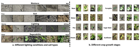
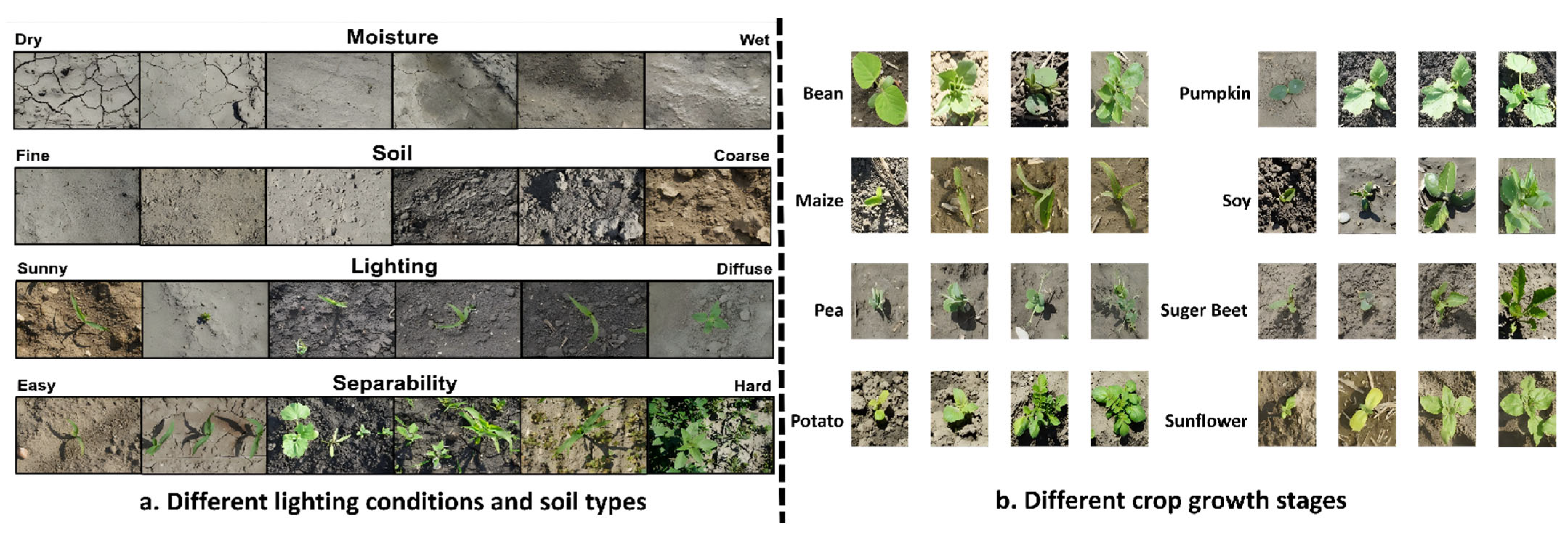
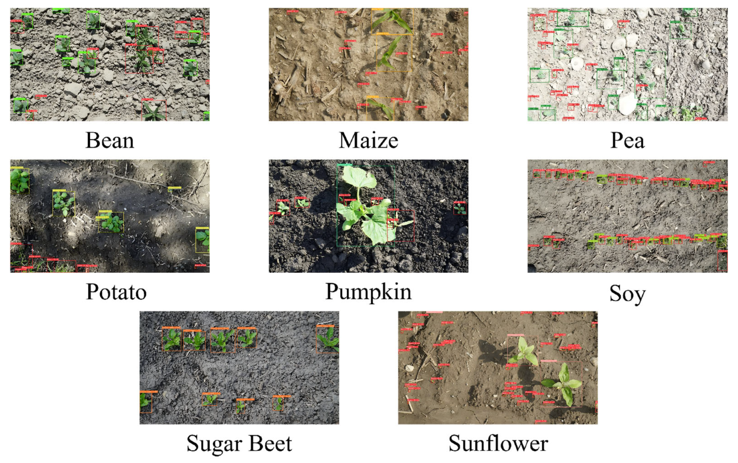
The training and evaluation of the model depend on the CropAndWeed dataset [18]. In precision agriculture, automated weed management requires a reliable visual reference. This dataset was selected for three main reasons. First, it is one of the largest publicly available agricultural datasets with per-instance bounding box annotations, containing 8369 images and 78,287 annotated instances across nine plant categories, which provides sufficient diversity for training deep detection models. Second, the images were captured under real farmland conditions with varying illumination, soil backgrounds, and plant densities, making it a representative benchmark for evaluating model robustness in practical agricultural scenarios. Third, its high-resolution images (1920 × 1080 pixels) retain fine morphological details of small vegetation, which is essential for developing and validating small-target detection capabilities required in early-stage weed control. These visual inputs cover diverse lighting conditions (from overcast to full sunlight), variable soil backgrounds (including dry cracked surfaces, wet muddy conditions, and sandy to loamy textures with varying granularity and moisture levels), and multiple plant growth stages spanning from the cotyledon stage to the 4–6 true-leaf vegetative stage (approximately BBCH 10–16).

Nine labeled plant categories were included in the experimental test. A wild plant category (weeds) was evaluated alongside eight standard crops. This plant list includes sunflower (Helianthus annuus L.), sugar beet (Beta vulgaris L.), maize (Zea mays L.), bean (Phaseolus vulgaris L.), potato (Solanum tuberosum L.), pea (Pisum sativum L.), pumpkin (Cucurbita pepo L.), and soybean (Glycine max (L.) Merr.). Figure 1 shows the real visual conditions of the farm. The background elements continue to change with the light level, soil humidity and surface cracking. The collected visual data also records different vegetation densities. Each marked plant category also covers multiple stages of growth and development.

Figure 1. Dataset introduction.

Researchers carefully filtered and merged the initially collected information. Our experimental procedures involved processing exactly 8369 images. Within this visual collection, 78,287 distinct bounding box instances were annotated. We subsequently partitioned the entire image corpus into three separate groups, which function as distinct training, validation, and testing components. Table 1 provides a comprehensive breakdown of how various plant classes are distributed. Obvious numerical disparities between categories occur throughout the database, paired with huge differences regarding actual object sizes.

Table 1. Dataset boundary box distribution.

Category	Train Set	Validation Set	Test Set	Total
Weed	40,300	5313	11,909	57,522
Sunflower	1379	157	343	1879
Sugar Beet	4468	435	1258	6161
Maize	4169	675	1174	6018
Bean	758	93	210	1061
Potato	265	36	70	371
Pea	454	77	90	621
Pumpkin	431	51	133	615
Soy	2826	429	784	4039

2.2. RT-BMTR Network Architecture

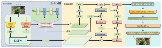
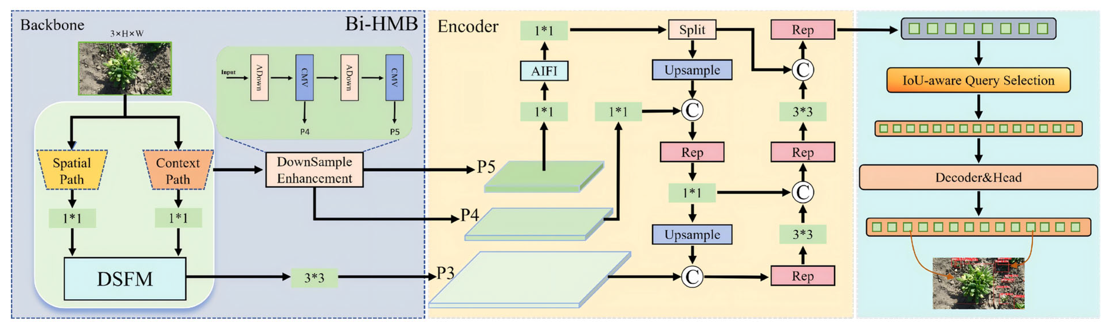
The RT-BMTR model targets plant detection across difficult agricultural environments. Target crops and wild species share almost identical leaf colors, surface textures, and physical shapes. Standard image recognition often fails due to the high similarity between crops and weeds. Newly grown weeds are easily obscured by complex soil backgrounds. Computational constraints present another challenge for standard field hardware. We used the RT-DETR network as our starting base. Continuous detection capabilities remain fully active within this framework. Specific structural updates enter the model through a modified backbone, an adjusted encoder, and a new loss function. Figure 2 illustrates the exact network layout.

Figure 2. RT-BMTR model. Note: 1 × 1 and 3 × 3 denote the corresponding convolution kernel sizes, Upsample denotes the upsampling operation, AIFI denotes the adaptive feature interaction module, and Rep denotes the RepNCSPELAN4 feature enhancement block.

As shown in the figure, the Bi-HMB backbone network receives the input image. Three sections form this core structure. These parts include a spatial path, a context path, and a detail–semantic fusion module (DSFM). Shallow convolution layers operate on the spatial branch. Image dimensions drop step by step in this area. Fine details like leaf edges and plant textures are protected by this action. The context branch works alongside it. Deep semantic features are extracted by the MambaVision module. Size reductions happen in this path as well. Outputs from both sides are fed into the DSFM. The fused feature P3 is created through this exact blend. Layer P3 maintains a high resolution. Small objects rely on the physical details saved in this layer. Multi-scale fusion operations build directly upon this base layer.

On this basis, deep features are extracted by downsampling modules within the backbone network. Layers P4 and P5 emerge from this exact process. Layer P4 functions as a middle stage. Physical details and semantic data are stored together in this map. Layer P5 carries deeper semantic traits along with an expanded receptive field. The model applies this specific layer to gather the full background context. Layers P3, P4, and P5 combine to build the final multi-scale output. The encoder module takes these maps directly to blend information across different sizes.

In the encoder, P3, P4, and P5 are sequentially processed through channel adjustment, AIFI, upsampling, concatenation, and Rep modules for feature fusion, forming a top-down semantic enhancement path. This is further combined with a bottom-up feature propagation process to achieve cross-scale information interaction. The Rep modules are introduced at each fusion node in the figure to reduce computational cost and latency while preserving feature representation capability.

In the detection head, the fused multi-scale features are passed to a decoder equipped with prediction heads to estimate the bounding box locations and object categories. For loss function design, this paper introduces Inner-ShapeIoU as the regression loss to strengthen the geometric constraints on small-target bounding boxes and improve the localization accuracy of tiny targets such as weed seedlings.

Overall, RT-BMTR is modified in three parts: the backbone network, the feature fusion module, and the loss function. The model diagram illustrates the connections between the modules and the flow of features throughout the network.

2.3. Bilateral Hybrid Backbone

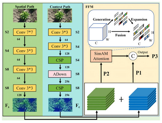
Young plants and wild grass share almost identical colors and leaf patterns in real field conditions. The physical sizes of these targets remain extremely tiny. Traditional convolutional neural networks lose image resolution as their processing layers deepen. This structural drop destroys the spatial data needed to find small objects. Pure Transformer architectures provide a global receptive field. However, high computational demands limit their real-time application on standard edge hardware. We built the Bi-HMB structure to solve these hardware and accuracy problems. Figure 3 illustrates this bilateral hybrid backbone network equipped with Mamba features. The layout contains a spatial path, a semantic path, and a feature fusion section. Standard 7 × 7 and 3 × 3 convolution layers drive the spatial branch through step-by-step size reduction. Spatial edges and visual patterns are preserved by this branch. The semantic path relies on parts like 3 × 3 convolutions, CSP, and ADown blocks. Deeper background context is pulled by the network through these elements. Information from both branches is fused in the DSFM block. This module creates the final multi-scale output.

Figure 3. Bi-HMB model.

2.3.1. Spatial Path

This paper introduces a spatial branch to focus on modeling the shallow feature level (P3). During downsampling to S8, the branch applies shallow convolutions to limit semantic compression. This preserves high-frequency structural details like seedling edges and leaf textures, providing stable support for subsequent feature fusion and object detection.

Specifically, the input image passes through four convolution layers with a stride of 2, namely 7 × 7, 3 × 3, 3 × 3, and 3 × 3, reducing the spatial resolution step by step to H/8 × W/8 while keeping the number of channels at 128, thereby obtaining the detail feature Fs. This design maintains a relatively high spatial resolution under a controllable computational cost, allowing local structures such as seedling edges and leaf veins to be clearly preserved. The computation process can be expressed as follows:

$$F_s={\mathsf{\varphi }}_{3\times 3}^{s2}\left({\mathsf{\varphi }}_{3\times 3}^{s2}\left({\mathsf{\varphi }}_{3\times 3}^{s2}\left({\mathsf{\varphi }}_{7\times 7}^{s2}\left(X\right)\right)\right)\right),$$

(1)

Among them, X represents the input image. The convolutional operation with a convolutional kernel size of 7 × 7 and a step length of 2 is represented by symbols ${\varphi }_{7\times 7}^{s2}(\cdot )$. The convolutional operation with a convolutional kernel size of 3 × 3 and a step length of 2 is also represented by the corresponding symbol ${\varphi }_{3\times 3}^{s2}(\cdot )$. The detailed feature diagram of the spatial branch output is marked as a specific symbol $F_s$. The superscript S2 indicates that the step length is 2, and the subscript indicates the size of the convolutional kernel.

The output Fs of this branch serves as the detailed input for subsequent fusion. It is aligned and fused with the semantic feature Fc from the semantic branch so that contextual information can be introduced while preserving fine-grained structures, thereby improving the discriminability and boundary localization accuracy of small targets.

2.3.2. Context Path

This study introduces a semantic branch called the context path in the backbone network. Progressive downsampling enlarges the receptive field while introducing long-range dependency modeling at higher layers. This enables the model to leverage both surrounding region information and global spatial distribution during discrimination. By not relying solely on local textures, the model improves its ability to distinguish between similar categories.

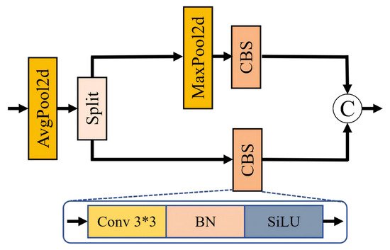
In order to reduce the damage of semantic branches to detailed information when downsampling, this paper introduces the ADown module.

Various processing units, including standard 3 × 3 convolutions, CSP, and Adown (Figure 4), handle the incoming data streams in a strict sequence. Physical image dimensions drop steadily during this phase to establish a broader conceptual understanding. The network simultaneously modifies the overall channel capacity to equal 256. We successfully obtained the required conceptual tensor designated as Fc through these exact mathematical steps. The computation process can be expressed as follows:

$$F_c={\psi }_{CSP}\left({\psi }_{ADown}\left({\psi }_{CSP}\left({\psi }_{3\times 3}\left({\psi }_{3\times 3}\left(X\right)\right)\right)\right)\right),$$

(2)

Figure 4. ADown model.

Among them, X represents the input feature. Convolutional operations with a convolutional kernel size of 3 × 3 are represented by specific symbols ${\psi }_{3\times 3}(\cdot )$. The CSP module is also referred to by a symbol ${\psi }_{CSP}(\cdot )$. ADown sub-sampling corresponds ${\psi }_{ADown}(\cdot )$. Fc represents the contextual feature diagram of the semantic branch output. The Fc output by the branch is aligned and fused with the spatial branch feature Fs as a semantic input for subsequent fusion. While retaining contextual information, this practice supplements the details of the fine-grained structure, thus improving the ability to distinguish small objects.

2.3.3. DownSample Enhancement

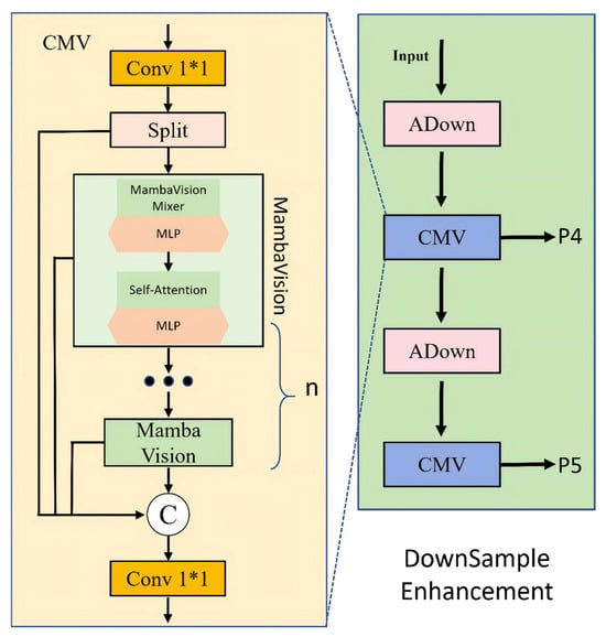
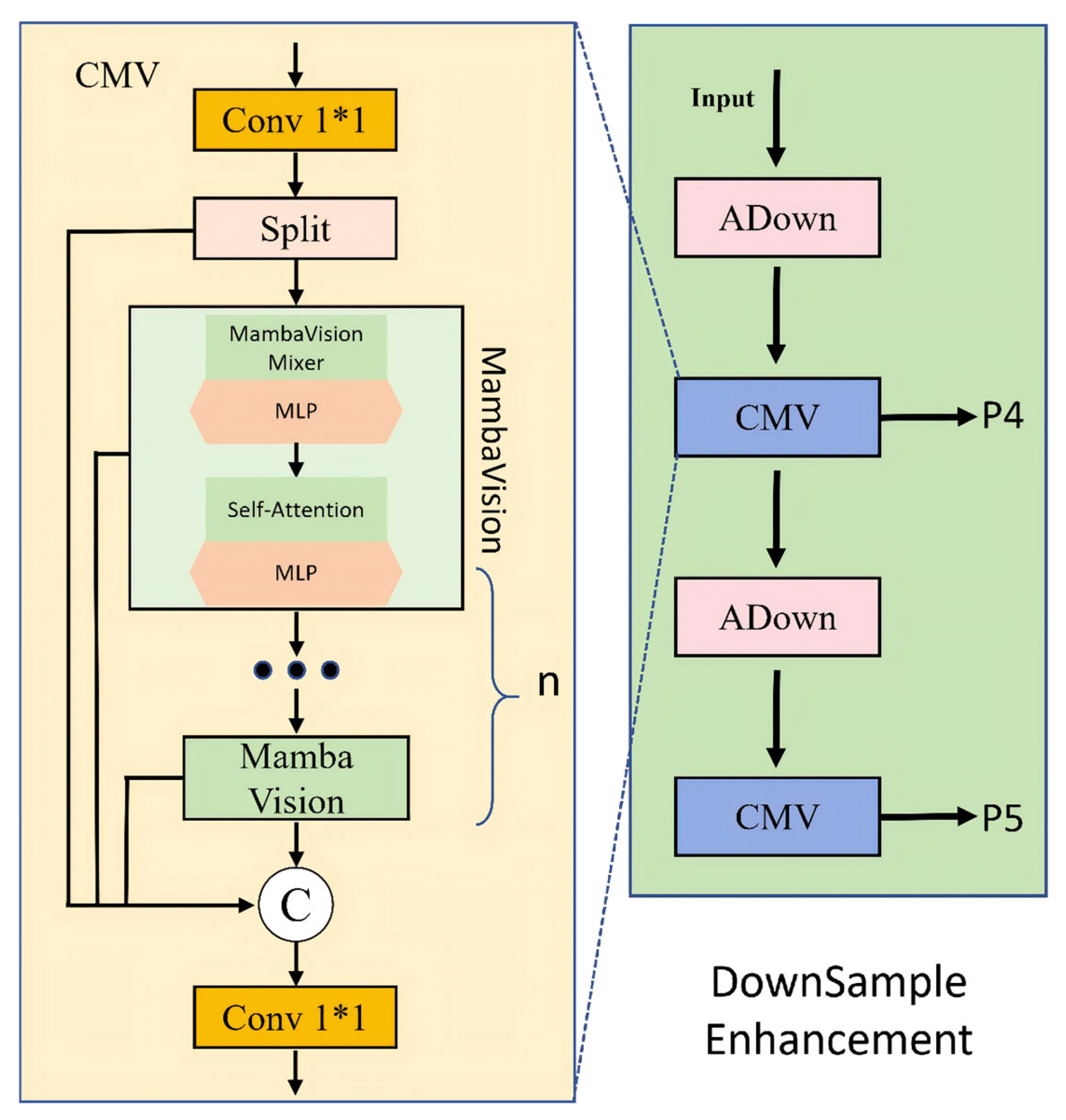
For crop and weed detection, the high similarity in color, texture, and morphology, together with interference from occlusion, illumination variation, and background noise, often results in both detail degradation and insufficient semantic discrimination during deep feature extraction. In farmland images, this problem is particularly pronounced at the seedling stage, where local textures are highly similar, and the target scale is small. If conventional downsampling is used alone, the feature maps not only lose resolution as the spatial dimension decreases but also tend to discard contextual information that is useful for subsequent discrimination. Taking these factors into account, we built a DownSample Enhancement unit into the size-reduction phase of the primary network, which is shown in Figure 5. This module improves feature representation while reducing spatial resolution. The CMV block serves as the main core of our design. Deep semantic information is extracted by this module to give the model the required background context.

Figure 5. DownSample Enhancement model.

We built the CMV block around selective state space models, generally known as SSMs. MambaVision acts as its main computational engine. Such a design allows the model to capture long-range relationships [19,20]. Its internal layout is divided into two parallel branches. Input features are split according to their channel dimensions. The first path preserves original data and guarantees smooth gradient flow. The remaining branch focuses entirely on deep feature extraction. Several MambaVision units operate here to learn complex visual patterns. After completing these steps, the model concatenates both data streams along the channel direction. A basic 1 × 1 convolution step finally mixes these parts to generate the exact required output.

$$h^{\prime }\left(t\right)=Ah\left(t\right)+Bx\left(t\right),$$

(3)

$$\mathrm{y}\left(\mathrm{t}\right)=\mathrm{C}\mathrm{h}\left(\mathrm{t}\right),$$

(4)

Crops and weeds are often very similar in local appearance, and it is difficult to distinguish them by texture or color alone, while global spatial distribution information often provides a more reliable basis for identification. CMV takes advantage of this point to combine local features with global contexts so that the model can still maintain good semantic recognition ability in complex contexts.

From the perspective of practical detection performance, this design is more suitable for agricultural images at the early seedling stage. At this stage, targets are small, and boundaries are weak. If semantic modeling is insufficient, the model may easily misclassify weeds as crops or produce missed detections under background interference. By supplementing contextual information during the downsampling stage through CMV, the DownSample Enhancement module can preserve effective features as much as possible while controlling computational cost, thereby providing more stable input for subsequent multi-scale fusion and laying a foundation for small-object detection.

2.3.4. DSFM

To address the loss of spatial information caused by the increasing depth of traditional convolutional neural networks, this study designs a feature fusion module named DSFM (detail–semantic fusion module). The module draws on the cross-stage partial connection idea of CSPNet and introduces a split-branch mechanism [21]. Specifically, the input feature map P is divided into two parts, P1 and P2, along the channel dimension. The P1 branch is directly passed through to preserve the original gradient information, while the P2 branch undergoes a series of dense convolution operations for deep feature transformation and abstract semantic extraction.

The DSFM architecture incorporates a series of compact residual units. Expanding the neural depth isolates more complex visual representations. Vanishing gradients are naturally prevented by shortcut paths during backpropagation. Field seedlings frequently cover merely a few dozen pixels within the input frames. Our module specifically targets the boundary details of these minute plants. Standard resolution reduction steps inherently discard vital spatial coordinates. The embedded residual structures successfully recover this absent geometric data. Upstream feature maps from both tracks are concatenated along their channel axis. A basic 1 × 1 convolution layer subsequently blends the combined tensor. We define this mathematical procedure below:

$$Y={\mathrm{C}\mathrm{o}\mathrm{n}\mathrm{v}}_{1\times 1}\left(\mathrm{C}\mathrm{o}\mathrm{n}\mathrm{c}\mathrm{a}\mathrm{t}\left(P_1,\mathrm{B}\mathrm{l}\mathrm{o}\mathrm{c}\mathrm{k}\left(P_2\right)\right)\right),$$

(5)

In this way, DSFM enhances the ability of shallow networks to capture fine-grained spatial information while maintaining computing efficiency.

2.4. RepNCSPELAN4-Based Feature Fusion Network

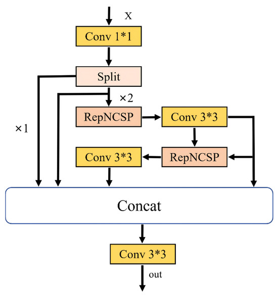
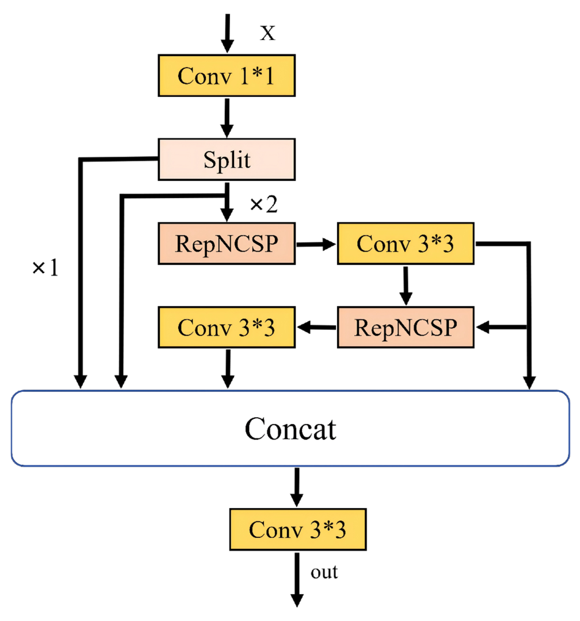
The hybrid encoder of RT-DETR undertakes the task of multi-scale feature fusion. In the farmland scene, the target scale changes greatly, the background interference is strong, and the computing resources deployed at the edge are also limited. In order to deal with these problems, this paper introduces the RepNCSPELAN4 module in the feature fusion stage. By combining GELAN’s gradient path design with structural re-parameterization, the module reduces computational cost while preserving feature representation capability [22].

Figure 6 presents the internal architecture. The RepNCSPELAN4 module utilizes a cross-stage partial configuration. Incoming feature tensors are partitioned into a bypass track and a primary processing track. Raw data representations remain intact within the bypass route. Gradients propagate smoothly through this specific path. Meanwhile, the processing track concentrates on deep visual pattern extraction. Standard ELAN networks typically stack basic convolution layers. The proposed dual-track layout avoids redundant mathematical operations. Tensor propagation across the computational graph strengthens simultaneously.

Figure 6. RepNCSPELAN4 model.

We incorporated the RepConv component directly within this processing unit. The model relies on a design with several parallel branches when the training process begins. A regular 3 × 3 convolution layer and a smaller 1 × 1 convolution layer are used here. An identity mapping provides the final shortcut. Implementing such parallel tracks greatly boosts the overall capacity regarding visual trait representation. During inference, the multi-branch structure is re-parameterized into a single 3 × 3 convolution. This reduces memory footprint and increases inference speed.

The cross-scale fusion process builds two distinct routing directions for tensor data. One track drives semantic enhancement from top to bottom. The other route refines spatial coordinates from bottom to top. The deep P5 tensor is initially expanded and merged alongside the P4 layer. This combined data interacts directly with the P3 level. Deep contextual meaning successfully reaches these early high-resolution visual grids. The model eventually reduces the spatial dimensions of these blended representations. These compacted tensors mix once more with deeper network levels. Structural boundaries and surface textures are effectively restored through this cyclic operation.

At each feature fusion node, the fusion process is expressed as follows:

$$F_{fusion}={\mathsf{\Phi }}_{Rep}\left(Concat\right(F_{low},Upsample\left(F_{high}\right)\left)\right),$$

(6)

where Φ_Rep denotes the nonlinear transformation of the Rep module.

2.5. Loss Function

Standard RT-DETR setups utilize the GIoU criterion [23] across the CropAndWeed dataset. The baseline model showed some limitations during the evaluation. The images we collected contain a huge number of tiny weeds. Standard methods usually measure positioning errors by looking at the smallest enclosing rectangle. Such evaluation metrics are simply insufficient for detecting small objects well enough. When the predicted area and the real target barely overlap, the loss values hardly change at all. This weak signal slows down the training process. Our new Bi-HMB main network works together with the RepNCSPELAN4 part to grab small visual details. The team had to introduce a better error formula to keep up with these improved feature extractions. We decided to use the Inner-ShapeIoU logic for the bounding box regression. This formula takes the size scaling from Inner-IoU and combines it with the shape and distance rules of Shape-IoU.

Our approach applies the Inner-IoU [24] method to create smaller helper boxes using a specific ratio factor. The model then calculates the overlap score right inside these shrunken boundaries. Setting the ratio to less than one automatically scales down both the predicted boxes and the ground-truth boxes at the same time. Scaling down the bounding boxes helps amplify the relative distance between them. The model can produce stronger gradient signals even when the boxes have limited overlap. This improves convergence during early training. We define the math for these inner boundaries as follows:

$$b_l^{inner}=x_c-{\displaystyle \frac{w \times ratio}{2}}{b}_l^{inner}=x_c-{\displaystyle \frac{w \times ratio}{2}},$$

(7)

$$b_r^{inner}=x_c+{\displaystyle \frac{w*ratio}{2}},$$

(8)

$$b_t^{inner}=y_c-{\displaystyle \frac{h*ratio}{2}},$$

(9)

$$b_b^{inner}=y_c+{\displaystyle \frac{h*ratio}{2}},$$

(10)

The variables x_c and y_c represent the center coordinates of the target, while w and h denote the width and height, respectively. These smaller inner boxes are then used by the network to compute the final overlap score.

Building on this logic, Shape-IoU [25] adds two extra penalties regarding shape and distance. This step keeps the geometric layout of the boxes in check. Traditional loss functions usually just focus on the overlapping area. Shape-IoU behaves differently during the evaluation process. It forces the predicted box to closely match both the aspect ratio and the center position of the real ground truth label. It is more effective to distinguish crops and weeds that are similar in appearance but slightly different in shape. Its shape and distance terms are as follows:

$$ww={\displaystyle \frac{2\cdot (w^{gt}{)}^{scale}}{(w^{gt}{)}^{scale}+(h^{gt}{)}^{scale}}},$$

(11)

$$hh={\displaystyle \frac{2\cdot (h^{gt}{)}^{scale}}{(w^{gt}{)}^{scale}+(h^{gt}{)}^{scale}}},$$

(12)

$$distance={\displaystyle \frac{hh\cdot (x_c-x_c^{gt}{)}^2+ww\cdot (y_c-y_c^{gt}{)}^2}{c^2}},$$

(13)

$$\mathsf{\Omega }={\sum _{t=w,h}\left(1-e^{-{\omega }_t}\right)}^4,$$

(14)

Within these established formulas, the scale parameter acts as a proportional multiplier. The mathematical symbol Ω functions to quantify geometric shape penalties. Our research group formulates the ultimate Inner-ShapeIoU error metric through the equation provided below:

$$L_{Inner-ShapeIoU}=1-Io{U}^{inner}+distance+0.5\cdot \mathsf{\Omega },$$

(15)

The Inner Shape-IoU loss function merges these exact mathematical concepts. Small targets still receive the strong gradient enhancements originally found in the Inner-IoU formula. The model also adopts the specific geometric rules of Shape-IoU to control the final bounding dimensions. Target coordinates achieve better precision directly through this combined methodology. Clustered weeds can be detected under difficult field conditions.

3. Experiment Results and Discussion

3.1. Experimental Conditions

A single computing architecture handles all model training and evaluation runs. Central processing relies on an Intel(R) Xeon(R) Platinum 8474C unit. Graphics calculations are executed by an NVIDIA GeForce RTX 4090D equipped with 24 GB of memory. Ubuntu 22.04 supplies the operating framework. Software dependencies include PyTorch 2.1.0, Python 3.10, and CUDA 12.1.

Visual inputs scale to 640 × 640 pixels prior to network initialization. Weight decay principles merge with an adaptive learning rate inside the AdamW optimizer. Mathematical convergence accelerates directly under this configuration. Final network weights tend to exhibit reliable generalization capabilities. Execution cycles run through 300 total epochs. A batch size of four regulates the continuous data flow. Four separate thread workers manage the memory loading tasks.

3.2. Indicator Selection

Model performance evaluation relies on the measurement standards established within the Microsoft COCO dataset [26]. Network behavior under variable agricultural conditions is assessed through this framework. Average precision serves as the primary metric for these evaluations. Recall and precision parameters are mathematically combined to generate this value. Varying confidence thresholds determine the resulting operational scores. Spatial overlap calculations depend entirely on the intersection over union mechanism. Predicted bounding boxes are measured against actual ground truth coordinates by this geometric operation. A standard 0.5 overlap requirement defines the AP⁵⁰ accuracy metric. This standard calculation easily shows how well the model locates basic objects. For the AP⁷⁵ metric, researchers set the exact overlap requirement to 0.75. The model must predict bounding boxes that closely match the ground truth to meet this criterion. The mAP^50–95 standard provides a much tougher test for bounding box accuracy. The model measures precision starting at a 0.5 baseline and goes up to 0.95. It uses a step size equal to 0.05 during this evaluation. We then average all these separate intermediate results together.

Crops and weeds change their physical sizes a lot as they grow. We applied different evaluation levels to deal with these shape differences. We followed the standard COCO rules to check the AP^S, AP^M, and AP^L scores. Precision (P) is defined as the proportion of correct predictions among all predicted bounding boxes (TP/(TP + FP)), while recall (R) is defined as the proportion of ground-truth objects that are successfully detected (TP/(TP + FN)). These two metrics are combined to compute average precision at each confidence threshold. These metrics show the detection performance on small, medium, and large objects. The defined pixel areas for these three categories fall strictly below 32², anywhere between 32² and 96², or anything above 96². Early-stage weeds usually take up very little space inside the pictures. Demonstrating success against such challenging visual elements verifies that our structural modifications genuinely function as intended. Field hardware generally operates under severe computational constraints. We therefore brought parameters alongside GFLOPs into the testing framework to quantify overall model complexity.

3.3. Backbone Network Comparison Experiment

To verify the effectiveness of the backbone network designed in this paper, representative backbone networks, namely RepViT, MobileNetV4, and ConvNeXtV2, were selected for comparison experiments. The baseline structure was swapped while keeping all learning parameters identical. Table 2 details the recorded performance variations. The new Bi-HMB architecture delivers higher scores across all primary evaluation standards. In particular, AP⁵⁰ reaches 66.3%, and AP^Small reaches 25.2%, both of which are higher than those of the other compared backbones. Bi-HMB also maintains strong competitiveness on medium- and large-object metrics, achieving 41.8% and 58.2%, respectively. Although Bi-HMB has a higher parameter count and computational cost than the lightweight backbones, with 21.0 M parameters and 90.1 GFLOPs, its improvement in overall detection accuracy is more significant. This suggests that the backbone enhances target representation capability through more comprehensive multi-scale feature modeling, with particularly prominent advantages in small-object recognition. Overall, Bi-HMB achieves a good balance between complexity and accuracy.

Table 2. Comparison of model training results using different backbone networks.

Backbone	FLOPS/G	Params/M	APSmall/%	APMedium/%	APLarge/%	AP50/%	P/%	R/%
Repvit	36.4	13.3	16.8	38.7	53.6	60.3	85.5	57.9
Mobilenetv4	39.5	11.3	23.0	43.4	58.4	65.9	85.4	63.4
Convnextv2	31.9	12.3	24.7	43.2	57.5	65.8	87.9	62.8
Bi-HMB	90.1	21.0	25.2	41.8	58.2	66.3	86.2	62.7

Note: Bold values indicate the best performance in each metric.

3.4. Ablation Experiment

We assessed the overall capabilities of the proposed architecture utilizing the validation split belonging to the CropAndWeed dataset. We thoroughly examined the basic structural layout alongside newly integrated processing units individually through targeted ablation experiments. Table 3 provides a complete breakdown detailing how these specific modifications influence general detection performance.

Table 3. Results of each improved ablation experiment.

No.	RT-DETR	Bi-HMB	Rep	Inner-ShapeIoU	P/%	R/%	AP50/%	AP75/%	AP50–95/%	APSmall/%	APMedium/%	APLarge/%	FLOPS/G	Params/M
1	√	×	×	×	86.6	62.7	65.5	53.3	49.7	22.8	42.7	57.8	57.0	19.8
2	√	√	×	×	86.2	62.7	66.3	53.5	50.1	25.2	41.8	58.2	90.1	21.0
3	√	√	√	×	87.1	64.3	67.6	54.7	51.0	24.5	44.2	59.7	54.6	13.9
4	√	√	√	√	86.5	65.3	68.1	54.8	50.9	26.5	44.7	59.3	54.6	13.9

Note: Bold values indicate the best performance in each metric. √ indicates the module/component is included; × indicates the module/component is not included.

The data proves that our new methods steadily upgrade the model performance when evaluated against the CropAndWeed images. We treated the first experiment as the base RT-DETR setup. Its basic AP50 metric stood at 65.5%. The model then captured an AP75 score of 53.3%. The combined AP50 to 95 evaluation returned exactly 49.7%. We also checked different target sizes. The AP^Small precision registered at 22.8%. The AP^Medium and AP^Large results reached 42.7% and 57.8%.

After introducing Bi-HMB on top of the baseline in Experiment 2, the detection performance improves: AP⁵⁰ rises to 66.3%, AP⁷⁵ to 53.5%, and AP^50–95 to 50.1%. In particular, the small-object metric AP^Small increases from 22.8% to 25.2%, a gain of 2.4% points, demonstrating the effectiveness of this module in multi-scale information interaction and detail feature preservation. Meanwhile, AP^Large also increases from 57.8% to 58.2%, indicating that this structure does not improve small-object performance at the expense of large-object detection. However, this stage also brings a certain increase in complexity, with FLOPs rising to 90.1 G and parameters increasing to 21.0 M, suggesting that feature enhancement alone increases inference burden.

To address the above issue, Experiment 3 further introduces RepNCSPELAN4 on top of Experiment 2. The results show that the model is optimized in both accuracy and efficiency. AP⁵⁰ increases to 67.6%, AP⁷⁵ rises to 54.7%, and AP^50–95 improves to 51.0%. In particular, AP^Medium and AP^Large increase to 44.2% and 59.7%, respectively, reflecting a further enhancement in the representation capability for medium- and large-scale targets. More importantly, FLOPs are dramatically reduced from 90.1 G to 54.6 G, and the parameter count drops from 21.0 M to 13.9 M, indicating that this module compresses redundant computation while maintaining accuracy gains and thus offers strong structural lightweighting value.

We evaluated our ultimate setup against the initial standard established during the first test. Three main accuracy scores were increased by 2.6, 1.5, and 1.2%. The network improved its small-target tracking by exactly 2.6%. We recorded the hardware demands during the fourth test. Total computing power was measured at 54.6 G. The overall model parameters remained at 13.9 M.

The results show that Bi-HMB, RepNCSPELAN4, and Inner-ShapeIoU work well together. The Bi-HMB structure improves how the network mixes features of different sizes. The RepNCSPELAN4 part keeps the mathematical processing fast without losing any precision. Finally, the Inner-ShapeIoU logic makes the bounding box placement much more reliable during training. Adding these pieces step by step raises overall scores. Finding very small weeds becomes much easier because of these changes. We also managed to keep the total model size and computing demands within strict limits. The CropAndWeed dataset testing fully supports these structural upgrades. This lightweight design is suitable for common farming hardware.

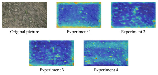
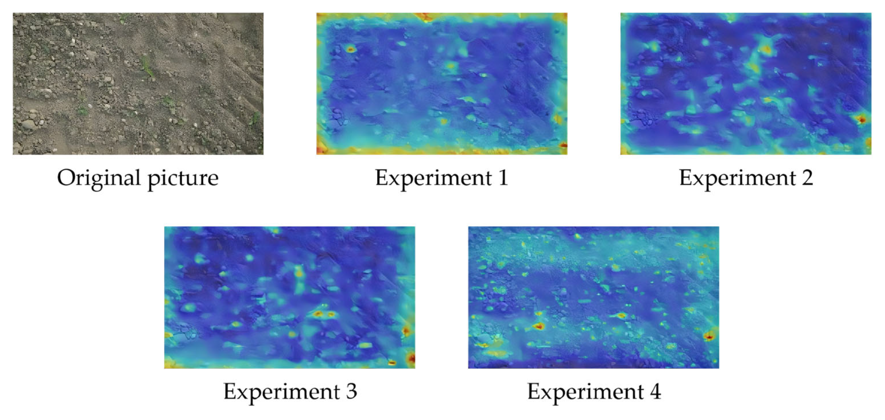
Figure 7 presents the original images alongside the corresponding heat maps for each experiment. The proposed methods change the regions of interest learned by the model. The baseline model is affected by soil patterns. Those early focus points end up being very messy and spread out. As the improved modules are gradually introduced, the high-response areas of the model begin to concentrate on target-related regions, and background interference is suppressed to a certain extent. In particular, in Experiment 4, the hotspot distribution becomes more continuous and more focused, indicating that this scheme can extract key features more effectively in complex field scenarios, thereby improving the discriminability of target regions and the stability of detection.

Figure 7. Ablation experiment heatmap.

3.5. Network Comparison Experiment

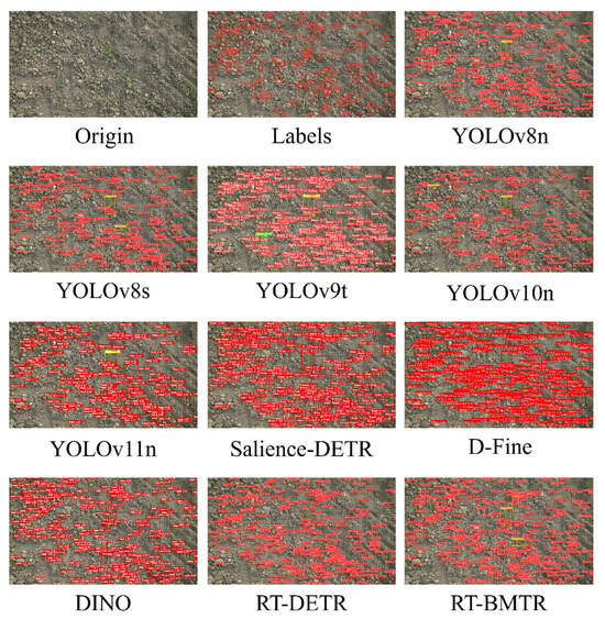
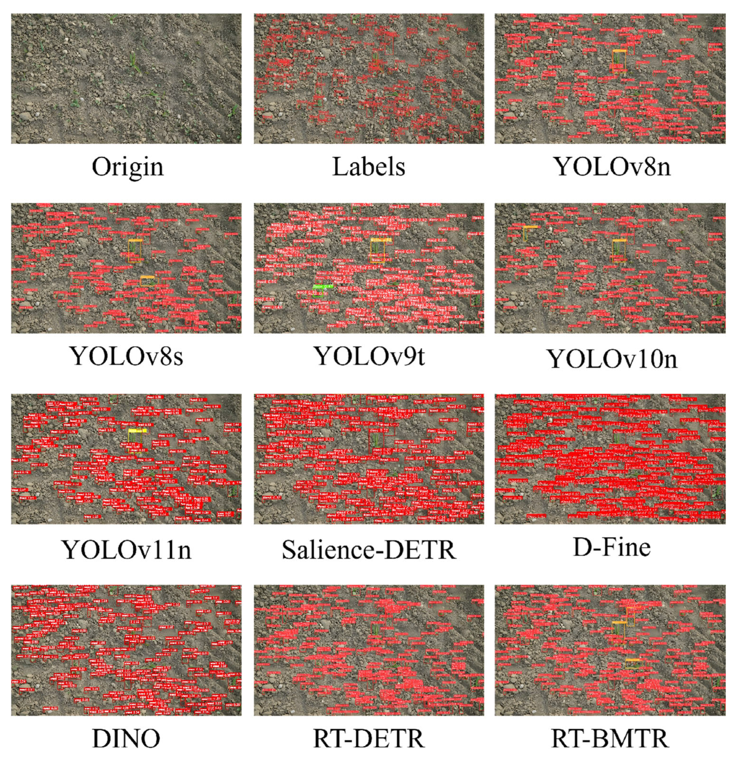
In order to verify the overall performance of the proposed model, this paper makes a horizontal comparison of RT-BMTR with several mainstream detectors. The results are shown in Table 4. The visualization examples are presented in Figure 8. RT-BMTR has achieved the best overall accuracy, with AP⁵⁰, AP⁷⁵ and AP^50–95 reaching 68.1%, 54.8% and 50.9% respectively, leading all comparison methods. In terms of small-target detection, RT-BMTR’s AP^Small reaches 26.5%, which is a great improvement compared with lightweight models such as YOLOv8n and YOLOv10n, and is also better than methods such as DINO and Salience-DETR. Under the background of disorder, the architecture can provide reliable visual characterization for tiny field targets. While dealing with these tiny targets, the RT-BMTR framework can also effectively handle standard-sized plants. According to the assessment index, its AP^Medium is 44.7% and AP^Large is 59.3%. When performing these tracking operations, the model fully retains the general identification ability. The directional structural adjustment for tiny vegetation has successfully avoided the decline in the overall accuracy of the network.

Table 4. Comparison of detection accuracy and computational cost across different object detectors.

Model	Backbone	AP50	AP75	AP50–95	APsmall	APmedium	APlarge	P/%	R/%	FLOPS/G	Parameters/M
YOLOv8n [27]	CSPDarkNet	66.5	53.4	49.7	22.3	44.0	58.9	80.8	63.0	6.8	2.7
YOLOv8s [27]	CSPDarkNet	67.1	54.7	50.1	23.9	45.5	58.3	85.2	63,5	28.5	11.1
YOLOv9t [28]	CSPBackbone	66.2	49.7	47.3	15.4	40.7	58.6	82.9	61.6	11.1	2.7
YOLOv10n [29]	CSPDarkNet	67.6	54.1	50.1	25.1	45.1	58.0	84.2	63.0	8.4	2.7
YOLOv11n [30]	CSPDarkNet	67.2	55.3	50.2	23.9	44.8	58.9	82.4	63.0	6.4	2.6
D-Fine [31]	HGNetv2	67.8	57.0	50.7	24.1	43.0	59.1	86.3	63.8	7.1	3.7
DINO [32]	Resnet50	64.3	52.3	48.1	23.6	43.0	56.3	64.3	72.5	279	47
Salience-DETR [33]	Resnet50	65.6	50.8	48.1	21.6	43.4	55.9	65.6	72.5	53	214.8
RT-DETR	Resnet18	65.5	53.3	49.7	22.8	42.7	57.8	85.6	62.7	57.0	19.9
RT-BMTR	Bi-HMB	68.1	54.8	50.9	26.5	44.7	59.3	86.5	65.3	54.6	13.9

Note: Bold values indicate the best performance in each metric.

Figure 8. Comparison of experimental results of different models.

The network has 13.9 M parameters and requires 54.6 G FLOPs of overall computational demand. Standard DETR frameworks, including DINO and Salience-DETR, generally require heavier processing loads compared to the RT-BMTR architecture. The model deployment on standard equipment remains highly practical under these physical constraints. Evaluation metrics yield a precision of 86.5% and a recall of 65.3%. With these values, the operating capacity of the model and the structural complexity have reached a functional balance. During field scanning, tiny invasive plants have become the focus of network attention, and standard crop tracking operations are also carried out synchronously without interference. In these two synchronous evaluations, AP^Medium remained at 44.7 and AP^Large reached 59.3. Judging from the comprehensive accuracy rate and recall rate score, the updated network fully retains the general plant recognition ability. Figure 9 shows the actual visual recognition process of the test field. In the face of different lighting conditions and crowded space conditions, the algorithm accurately tracks the target boundary. The complex background interference was suppressed by the model in the final calculation, and the small blade edge coordinates were extracted directly from the filtered visual data.

Figure 9. Visualization of major crop detection.

The comparative evaluation establishes the core competence of the RT-BMTR model. The model achieved the best results in the three evaluation criteria of AP⁵⁰, AP⁷⁵ and AP^50–95. In these tests, the AP^Small indicator achieved direct growth in terms of numbers. This structural configuration can separate tiny visual targets from the messy field background. During the whole operation process, the total number of network parameters and the computing processing requirements are controlled. Compared with the standard DETR framework, the practicality of model deployment has been enhanced under these physical hardware conditions. Its recognition accuracy, physical scale adjustment and model workload have reached a functional balance. Based on these verified network improvements, the deployment of actual field applications has become a realistic choice.

From an agronomic perspective, the improved detection of small weeds at early growth stages is particularly valuable, as this coincides with the critical period for weed control—removing weeds after this window results in irreversible yield loss. The model’s ability to maintain reliable detection across diverse soil and lighting conditions further supports its practical deployment in real farming operations, where environmental variability is the norm rather than the exception.

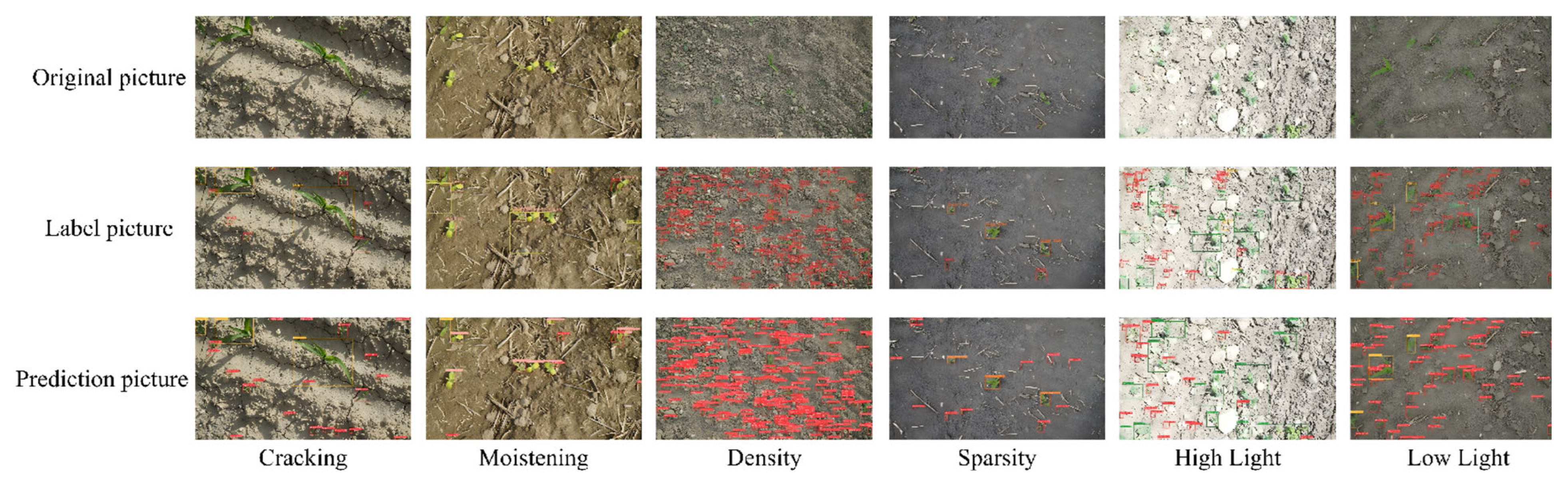
3.6. Detection Results in Different Scenarios

Varied agricultural environments test the adaptability of the RT-BMTR framework. The test scenarios included dry, cracked soil and wet mud. Image recognition was evaluated on isolated plants and weeds clumped tightly together. Bright sunlight and deep shadows provided strong lighting challenges for the camera. Figure 10 shows how the network still accurately spots crops and weeds under most of these tricky conditions. Intense illumination occasionally creates localized blown-out spots plus irregular shading. These specific optic flaws degrade crucial surface details alongside boundary sharpness. Such physical degradation eventually triggers false-positive alerts while causing other targeted objects to be completely overlooked across certain patches.

Figure 10. Detection effect diagrams under different scenarios.

3.7. RT-BMTR Limitation Analysis

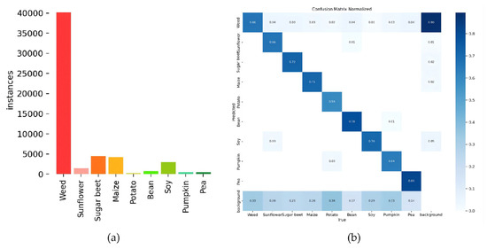
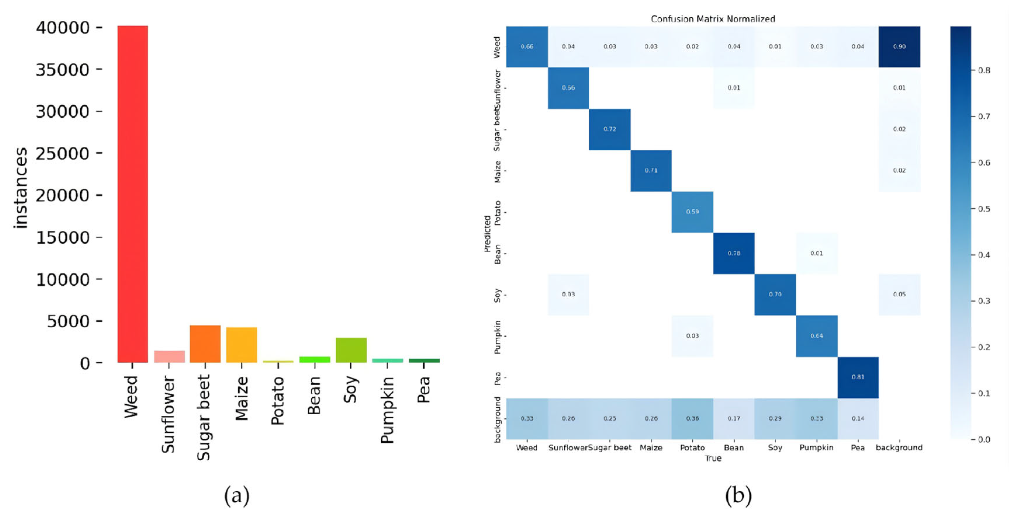
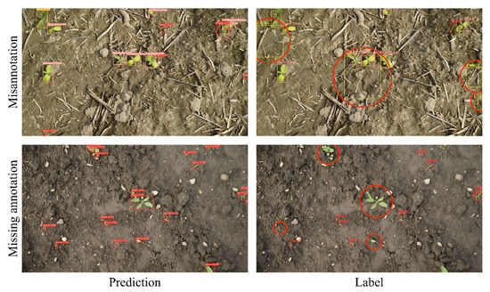
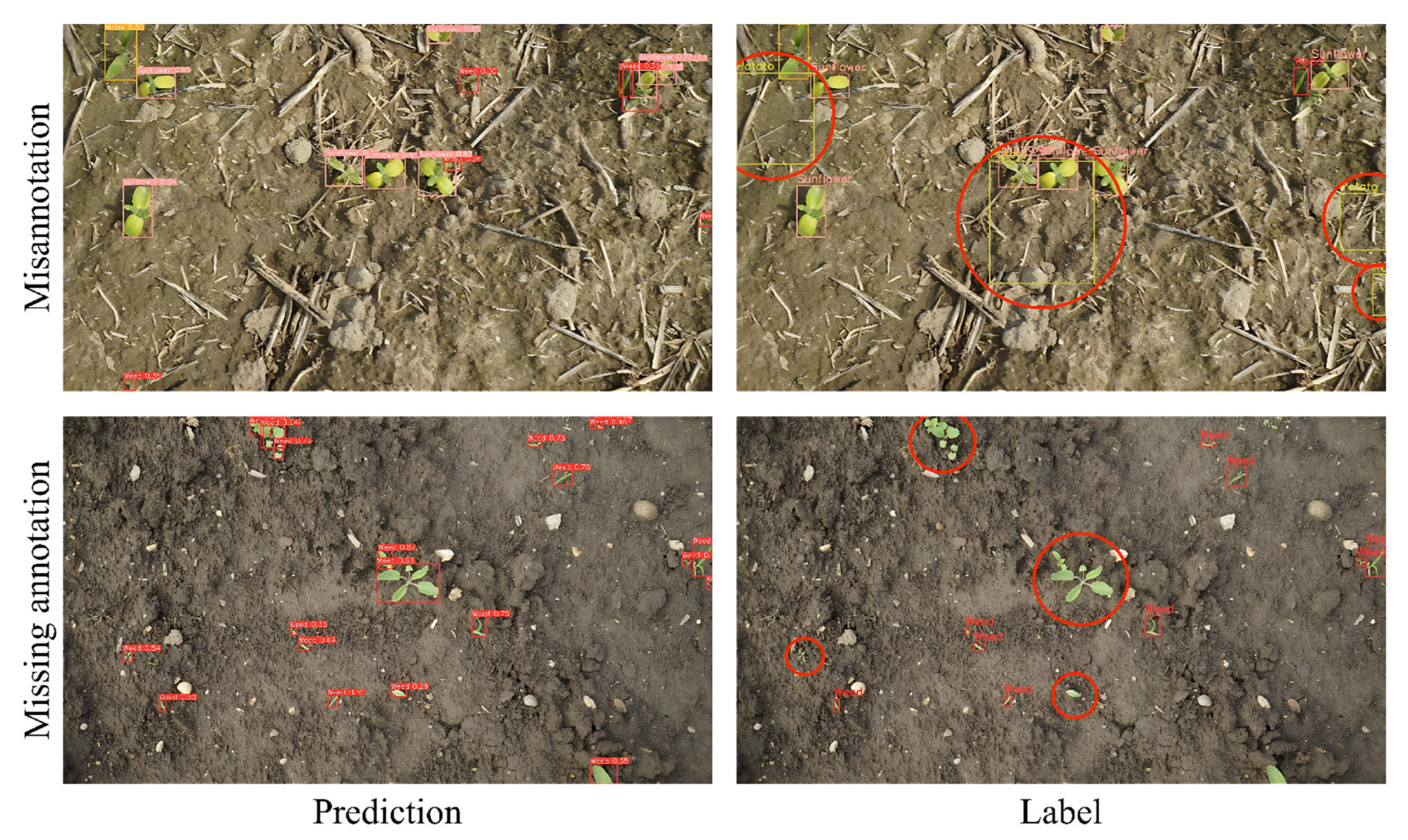
This paper uses a confusion matrix to visually evaluate the detection results of different categories. As shown in Figure 11b, the model shows an overall similar recognition capability across most categories, while the detection performance for potatoes is relatively weaker. At the same time, all crop categories suffer from varying degrees of missed detection, among which weed-related false detections are particularly prominent, reaching 90%. Further analysis based on the dataset annotation statistics shows that this phenomenon is not entirely caused by the model itself, but is also closely related to data quality: on the one hand, weed samples contain missing annotations, which weakens the model’s learning of real weed features. On the other hand, some crop labels are incorrectly annotated, for example, blank regions being labeled as crops, which causes the boundary between background and crops to be artificially narrowed, as shown in Figure 12. In addition, the category distribution is highly imbalanced, as shown in Figure 11a, where the number of weed samples is far greater than that of other categories, and the insufficient number of potato samples further amplifies the model’s bias toward high-frequency categories. Overall, the current results reflect the combined effect of model performance and annotation noise. In the future, annotation cleaning and class balancing will be carried out to obtain more reliable evaluation results.

Figure 11. Label statistics (a) and confusion matrix (b).

Figure 12. Misannotation and missing annotation. Note: In the label diagram, the red circles mark the regions of misannotation and missing annotation.

4. Conclusions and Future Work

To address the multiple challenges present within agricultural environments prior to removing invasive plants, we developed an upgraded architecture named RT-BMTR, which builds directly upon the foundational RT-DETR layout. These problems include: the large number of weeds and the competition for growth space with crop seedlings, the large changes in the target scale, and the strong background interference. With the help of Bi-HMB, a bilateral hybrid network, the model enhances the synergistic characterization of local details and global semantics. In the feature fusion network, RepNCSPELAN4 is introduced to reduce computational redundancy, while the Inner-ShapeIoU regression strategy strengthens the positioning ability of densely distributed small targets.

Experiments on the CropAndWeed dataset show the good detection accuracy and efficiency of our RT-BMTR architecture. Specific evaluation scores recorded 68.1% for AP⁵⁰, followed by 54.8% for AP⁷⁵, plus an overall AP^50–95 of 50.9%. Evaluating different physical dimensions yielded 26.5% for AP^Small, 44.7% for AP^Medium, and 59.3% for AP^Large. When evaluated against the original RT-DETR foundation, our upgraded framework significantly overcomes previous limitations in small-object detection. We simultaneously shrank overall mathematical parameters down to 13.9 M while reducing processing demands to exactly 54.6 G. Such hardware efficiency guarantees highly practical field deployment. The proposed method improves the detection of small weeds while maintaining stable performance on medium and large objects.

Nevertheless, the model still has room for further improvement under extreme illumination, severe occlusion, and imbalanced class distribution conditions. Future work will focus on three aspects: (1) model compression for deployment on low-power embedded devices; (2) annotation refinement to address class imbalance and improve detection reliability (strategies such as active learning with human-in-the-loop verification, semi-supervised annotation cleaning, and class-aware data augmentation can be explored for this purpose); and (3) cross-region data collection for enhanced generalization across diverse field environments.

References

- Slaughter, D.C.; Giles, D.K.; Downey, D. Autonomous robotic weed control systems: A review. Comput. Electron. Agric. 2008, 61, 63–78. [Google Scholar] [CrossRef] [Scilit]
- Westwood, J.H.; Charudattan, R.; Duke, S.O.; Fennimore, S.A.; Marrone, P.; Slaughter, D.C.; Swanton, C.; Zollinger, R. Weed management in 2050: Perspectives on the future of weed science. Weed Sci. 2018, 66, 275–285. [Google Scholar] [CrossRef] [Scilit]
- Yang, Z.; Zhang, W.; Hu, C.; Feng, Z.; Li, J. RDD-DETR Algorithm for Full-Scale Detection of Rice Diseases. Agriculture 2026, 16, 799. [Google Scholar] [CrossRef] [Scilit]
- Kamilaris, A.; Prenafeta-Boldú, F.X. Deep learning in agriculture: A survey. Comput. Electron. Agric. 2018, 147, 70–90. [Google Scholar] [CrossRef] [Scilit]
- Olsen, A.; Konovalov, D.A.; Philippa, B.; Ridd, P.; Wood, J.C.; Johns, J.; Banks, W.; Girgenti, B.; Kenny, O.; Whinney, J.; et al. DeepWeeds: A multiclass weed species image dataset for deep learning. Sci. Rep. 2019, 9, 2058. [Google Scholar] [CrossRef] [Scilit] [PubMed]
- Ren, S.; He, K.; Girshick, R.; Sun, J. Faster R-CNN: Towards real-time object detection with region proposal networks. IEEE Trans. Pattern Anal. Mach. Intell. 2017, 39, 1137–1149. [Google Scholar] [CrossRef] [Scilit] [PubMed]
- Zhang, X.; Cui, J.; Liu, H.; Han, Y.; Ai, H.; Dong, C.; Zhang, J.; Chu, Y. Weed Identification in Soybean Seedling Stage Based on Optimized Faster R-CNN Algorithm. Agriculture 2023, 13, 175. [Google Scholar] [CrossRef] [Scilit]
- Dos Santos Ferreira, A.; Freitas, D.M.; da Silva, G.G.; Pistori, H.; Folhes, M.T. Weed detection in soybean crops using ConvNets. Comput. Electron. Agric. 2017, 143, 314–324. [Google Scholar] [CrossRef] [Scilit]
- Zhang, R.; Wang, C.; Hu, X.; Liu, Y.; Chen, S.; Su, B. Weed location and recognition based on UAV imaging and deep learning. Int. J. Precis. Agric. Aviat. 2020, 3, 23–29. [Google Scholar] [CrossRef] [Scilit]
- Wang, C.-Y.; Bochkovskiy, A.; Liao, H.-Y.M. Scaled-YOLOv4: Scaling cross stage partial network. In Proceedings of the IEEE/CVF Conference on Computer Vision and Pattern Recognition (CVPR), Nashville, TN, USA, 20–25 June 2021; IEEE: New York, NY, USA, 2021; pp. 13029–13038. [Google Scholar]
- Wang, Q.; Cheng, M.; Huang, S.; Cai, Z.; Zhang, J.; Yuan, H. A deep learning approach incorporating YOLO v5 and attention mechanisms for field real-time detection of the invasive weed Solanum rostratum Dunal seedlings. Comput. Electron. Agric. 2022, 199, 107194. [Google Scholar] [CrossRef] [Scilit]
- Jin, X.; Che, J.; Chen, Y. Weed identification using deep learning and image processing in vegetable plantation. IEEE Access 2021, 9, 10940–10950. [Google Scholar] [CrossRef] [Scilit]
- Touvron, H.; Cord, M.; Douze, M.; Massa, F.; Sablayrolles, A.; Jégou, H. Training data-efficient image transformers & distillation through attention. In Proceedings of the International Conference on Machine Learning (ICML), Vienna, Austria, 18–24 July 2021; pp. 10347–10357. [Google Scholar]
- Wang, W.; Xie, E.; Li, X.; Fan, D.-P.; Song, K.; Liang, D. Pyramid vision transformer: A versatile backbone for dense prediction without convolutions. In Proceedings of the IEEE/CVF International Conference on Computer Vision (ICCV), Montreal, QC, Canada, 10–17 October 2021; IEEE: New York, NY, USA, 2021; pp. 568–578. [Google Scholar]
- Zhu, X.; Su, W.; Lu, L.; Li, B.; Wang, X.; Dai, J. Deformable DETR: Deformable transformers for end-to-end object detection. In Proceedings of the International Conference on Learning Representations (ICLR), Virtual Only Conference, 3–7 May 2021. [Google Scholar]
- Reedha, R.; Dericquebourg, E.; Canals, R.; Hafiane, A. Transformer neural network for weed and crop classification of high resolution UAV images. Remote Sens. 2022, 14, 592. [Google Scholar] [CrossRef] [Scilit]
- Zhao, Y.; Lv, W.; Xu, S.; Wei, J.; Wang, G.; Dang, Q.; Liu, Y.; Chen, J. DETRs beat YOLOs on real-time object detection. In Proceedings of the IEEE/CVF Conference on Computer Vision and Pattern Recognition (CVPR), Seattle, WA, USA, 16–22 June 2024; IEEE: New York, NY, USA, 2024; pp. 16965–16974. [Google Scholar]
- Steininger, D.; Trondl, A.; Croonen, G.; Simon, J.; Widhalm, V. The CropAndWeed Dataset: A Multi-Modal Learning Approach for Efficient Crop and Weed Manipulation. In Proceedings of the IEEE/CVF Winter Conference on Applications of Computer Vision (WACV), Waikoloa, HI, USA, 2–7 January 2023; IEEE: New York, NY, USA, 2023; pp. 3729–3738. [Google Scholar]
- Gu, A.; Dao, T. Mamba: Linear-time sequence modeling with selective state spaces. In Proceedings of the First Conference on Language Modeling (COLM), Philadelphia, PA, USA, 7–9 October 2024. [Google Scholar]
- Hatamizadeh, A.; Kautz, J. MambaVision: A hybrid Mamba-transformer vision backbone. In Proceedings of the IEEE/CVF Conference on Computer Vision and Pattern Recognition (CVPR), Nashville, TN, USA, 15–20 June 2025; IEEE: New York, NY, USA, 2025; pp. 25261–25270. [Google Scholar]
- Wang, C.Y.; Liao, H.Y.M.; Wu, Y.H.; Chen, P.-Y.; Hsieh, J.-W.; Yeh, I.-H. CSPNet: A new backbone that can enhance learning capability of CNN. In Proceedings of the IEEE/CVF Conference on Computer Vision and Pattern Recognition Workshops (CVPRW), Seattle, WA, USA, 14–19 June 2020; IEEE: New York, NY, USA, 2020; pp. 1571–1580. [Google Scholar]
- Ding, X.; Zhang, X.; Ma, N.; Han, J.; Ding, G.; Sun, J. RepVGG: Making VGG-style ConvNets great again. In Proceedings of the IEEE/CVF Conference on Computer Vision and Pattern Recognition (CVPR), Nashville, TN, USA, 20–25 June 2021; IEEE: New York, NY, USA, 2021; pp. 13733–13742. [Google Scholar]
- Rezatofighi, H.; Tsoi, N.; Gwak, J.; Sadeghian, A.; Reid, I.; Savarese, S. Generalized intersection over union: A metric and a loss for bounding box regression. In Proceedings of the IEEE/CVF Conference on Computer Vision and Pattern Recognition (CVPR), Long Beach, CA, USA, 15–20 June 2019; IEEE: New York, NY, USA, 2019; pp. 658–666. [Google Scholar]
- Zhang, H.; Xu, C.; Zhang, S. Inner-IoU: More effective intersection over union metric with auxiliary bounding box. arXiv 2023, arXiv:2311.02877. Available online: https://arxiv.org/abs/2311.02877 (accessed on 10 May 2026).
- Zhang, H.; Zhang, S. Shape-IoU: More accurate metric considering bounding box shape and scale. arXiv 2023, arXiv:2312.17663. Available online: https://arxiv.org/abs/2312.17663 (accessed on 10 May 2026).
- Lin, T.Y.; Maire, M.; Belongie, S.; Hays, J.; Perona, P.; Ramanan, D.; Dollár, P.; Zitnick, C.L. Microsoft COCO: Common objects in context. In Proceedings of the European Conference on Computer Vision (ECCV), Zurich, Switzerland, 6–12 September 2014; pp. 740–755. [Google Scholar]
- Jocher, G.; Chaurasia, A.; Qiu, J.; Burhan, M.; Stoken, A.; Borovec, J.; Kwon, Y.; Michael, K.; Fang, J.; Wong, C.; et al. Ultralytics YOLOv8. Available online: https://github.com/ultralytics/ultralytics (accessed on 8 May 2026).
- Wang, C.Y.; Yeh, I.H.; Liao, H.Y.M. YOLOv9: Learning what you want to learn using programmable gradient information. In Proceedings of the IEEE/CVF Conference on Computer Vision and Pattern Recognition (CVPR), Seattle, WA, USA, 16–22 June 2024; IEEE: New York, NY, USA, 2024; pp. 16223–16232. [Google Scholar]
- Wang, A.; Chen, H.; Liu, L.; Chen, K.; Lin, Z.; Han, J.; Ding, G. YOLOv10: Real-time end-to-end object detection. In Proceedings of the Advances in Neural Information Processing Systems (NeurIPS), Vancouver, BC, Canada, 10–15 December 2024. [Google Scholar]
- Ultralytics. YOLO11. Available online: https://docs.ultralytics.com/models/yolo11/ (accessed on 8 May 2026).
- Peng, Y.; Li, H.; Wu, P.; Zhang, Y.; Sun, X.; Wu, F. D-FINE: Redefine Regression Task of DETRs as Fine-grained Distribution Refinement. In Proceedings of the International Conference on Learning Representations (ICLR), Singapore, 24–28 April 2025. [Google Scholar]
- Zhang, H.; Li, F.; Liu, S.; Zhang, L.; Su, H.; Zhu, J.; Ni, L.M.; Shum, H.-Y. DINO: DETR with improved de-noising anchor boxes for end-to-end object detection. In Proceedings of the International Conference on Learning Representations (ICLR), Kigali, Rwanda, 1–5 May 2023. [Google Scholar]
- Hou, X.; Liu, M.; Zhang, S.; Wei, P.; Chen, B. Salience DETR: Enhancing detection transformer with hierarchical salience filtering refinement. In Proceedings of the IEEE/CVF Conference on Computer Vision and Pattern Recognition (CVPR), Seattle, WA, USA, 17–21 June 2024; IEEE: New York, NY, USA, 2024; pp. 17565–17574. [Google Scholar]
Disclaimer/Publisher’s Note: The statements, opinions and data contained in all publications are solely those of the individual author(s) and contributor(s) and not of MDPI and/or the editor(s). MDPI and/or the editor(s) disclaim responsibility for any injury to people or property resulting from any ideas, methods, instructions or products referred to in the content. |
© 2026 by the authors. Licensee MDPI, Basel, Switzerland. This article is an open access article distributed under the terms and conditions of the Creative Commons Attribution (CC BY) license.