


Abstract
Deep stormwater drainage tunnels are increasingly being used to mitigate urban flooding, but in-tunnel sediment deposition reduces their discharge capacity and complicates their maintenance. With direct field observation constrained, numerical simulation is essential, and river-based total sediment load formulas require reassessment for use in deep tunnels. The three-phase (air–water–sediment) CFD solver SedInterFoam is first validated against a benchmark open-channel suspended sediment experiment, and is then applied to a horseshoe tunnel under a fixed design discharge for multiple inlet sediment concentrations spanning urban stormwater conditions. Four classical formulas (Yang, Shen–Hung, Ackers–White, Engelund–Hansen) are evaluated at the CFD-resolved hydraulic state; Toffaleti is omitted because its zone-based formulation is incompatible with the partially filled horseshoe geometry. The CFD consistently shows persistent retention of a substantial fraction of the inlet sediment load, whereas the transport capacity-limited interpretation of the classical formulas predicts near-complete sediment throughput—indicating structural inadequacy for the dilute, supply-limited regime typical of urban stormwater. A Universal Soil Loss Equation (USLE)-style dimensionless deposition formula is therefore proposed, with inlet sediment loading as the explicit independent variable and a tunnel correction factor absorbing the geometric, hydraulic, and sediment variations. Its regression yields an almost linear scaling and a nearly constant deposition ratio, while analysis of the internal flow and concentration fields shows that the retained sediment is strongly concentrated near the bed and that near-bed turbulent mixing weakens moderately with a rising inlet concentration. While calibrated for a single non-cohesive settleable sand fraction, the framework provides a transferable basis for inlet-loading-dependent deposition prediction in deep stormwater drainage tunnels, and subsequent extension of to broader sediment conditions with field-based validation is expected to enable maintenance planning, dredging volume estimation, and sediment retention risk assessment.
1. Introduction
Urban flooding is increasingly motivating the construction of deep stormwater drainage tunnels in dense urban areas where conventional surface-based flood control measures are difficult to implement. Conventional measures, such as levee reinforcement and river expansion, are often constrained by limited surface space; therefore, deep stormwater drainage tunnels are increasingly being used to bypass and drain large flood volumes. These tunnels are characterized by rapid head changes, large diameters, long flow distances, and intermittent operation. Similar operational characteristics have been documented in international deep storage tunnel systems, including the Chicago Tunnel and Reservoir Plan (TARP) and DC Water’s deep tunnel system, where the transient flow regimes between free-surface and pressurized states have been identified as recurring design challenges [1].
Under these operating conditions, settleable sediment can progressively accumulate in the central tunnel and outlet sections, reducing the discharge capacity and increasing maintenance costs [2,3]. Sediment management in deep stormwater drainage tunnels is particularly difficult because the tunnel depth, length, limited access, and high dredging costs restrict direct inspection and dredging operations. These constraints highlight the need for predictive tools that can estimate sediment transport and deposition before maintenance problems develop. Because field observation alone is limited by spatial accessibility, safety concerns, and the cost of long-term monitoring, numerical models that can resolve the free-surface multiphase flow can provide a practical alternative for predicting sediment behavior in inaccessible tunnel environments.
Previous sewer flow studies have demonstrated that computational fluid dynamics (CFD)-based models can reproduce free-surface sediment transport, deposited bed evolution, and particle–flow interactions [4,5,6]. However, these studies mainly targeted sewer or partial-flow pipe systems rather than large-scale deep stormwater drainage tunnels with intermittent operation, rapid hydraulic transitions, and limited field accessibility. The studies specifically addressing deep stormwater drainage tunnels have mainly focused on system optimization, inflow capacity, route planning, air entrainment, and ventilation under water–air two-phase flow conditions [7,8,9]. Sediment-related design studies have also examined non-deposition or self-cleansing thresholds [10], but few studies have directly linked three-phase CFD results to tunnel-specific deposition rate prediction, particularly under partial-throughput conditions in which only part of the inlet sediment load exits the tunnel while the remaining fraction is deposited within the tunnel reach. This gap motivates the use and validation of a three-phase CFD solver capable of simultaneously resolving the free-surface motion, sediment suspension, deposition, and near-bed transport.
During a flood event, the main-line tunnel evolves from a partially filled Free stage to a Transition stage and eventually to a Submerged stage as the downstream head rises (Figure 1). In the Free stage, the tunnel behaves as an atmosphere-vented open channel, and sediment is transported primarily in suspension. This study focuses on the Free stage because it provides the most appropriate conditions for comparing CFD-predicted sediment throughput with total sediment load formulas. The computational domain is therefore interpreted as a representative straight segment of the main-line tunnel under Free stage operation.
Figure 1.
Evolution of hydraulic states in the main-line of a deep stormwater drainage tunnel. (a) Free stage: Partially filled open-channel flow; sediment carried in suspension (present study’s scope). (b) Transition: Rising downstream head forms a hydraulic jump that migrates upstream. (c) Submerged stage: Free surface is suppressed; settling and bottom deposition dominate (outside the present scope).
In addition to the lack of three-phase tunnel-scale deposition modeling, another key issue concerns the total sediment load formulas traditionally used to estimate transport capacity in sewer and tunnel design. These formulas were originally developed for natural alluvial rivers with mobile beds, bed forms, and simplified laboratory channel geometries. Applying such formulas to concrete-lined, fixed-bed, non-rectangular deep stormwater drainage tunnels by simple variable substitution can be physically inconsistent unless the underlying assumptions are reformulated. Beyond these geometric and boundary condition differences, the operational sediment supply regime of deep stormwater drainage tunnels also differs fundamentally from that assumed in classical river formulas. Even after formula-specific adaptation of river-based assumptions to tunnel-consistent variables, the governing framework of these formulas remains problematic for deep-tunnel operation. Classical total sediment load formulas predict a single transport capacity independent of inlet sediment loading, under the implicit assumption that the imposed sediment supply approaches or exceeds the capacity. This condition is referred to here as the transport capacity-limited regime. However, the sediment supply entering deep stormwater drainage tunnels during urban runoff events is generally far below such a capacity-limited condition. The event-mean suspended solids concentrations in Korean urban road runoff have been reported to be on the order of 30–130 mg/L, with the first-flush peaks occasionally reaching 1000–1500 mg/L [11,12,13]. Under these dilute, supply-limited conditions, deposition is expected to scale with inlet loading rather than with the formal transport capacity. The classical transport capacity-limited framework is therefore structurally inappropriate for the operational concentration range of deep stormwater drainage tunnels, and a deposition rate formulation that takes inlet sediment loading as an explicit independent variable is required.
Accordingly, the present study is structured around three coupled contributions. First, the OpenFOAM-based SedInterFoam solver is validated by reproducing the Coleman [14] benchmark open-channel suspended sediment laboratory experiment. The logarithmic velocity distribution, Rouse-type concentration distribution, and Meyer–Peter and Müller [15] bed load prediction are used as quantitative benchmarks, providing a physically grounded basis for applying the same solver to tunnel domains. Second, five classical total sediment load formulas [16,17,18,19,20] are reviewed by examining their underlying assumptions; four of them are then evaluated at the non-uniform partially filled hydraulic state measured from the CFD simulation. The Yang, Ackers–White, and Engelund–Hansen formulas are quantitatively compared with the CFD outlet sediment flux, whereas the Shen–Hung is treated as a calibration envelope diagnostic and Toffaleti is excluded from the quantitative comparison because its vertical-integration structure is not directly applicable to a partially filled horseshoe cross-section. Through this comparison, the transport capacity-limited framework underlying the classical formulas is shown to be structurally inadequate for the realistic operational concentration range.
Third, the validated solver is applied to a horseshoe-shaped cross-section representative of deep stormwater drainage tunnels operating in South Korea. The simulations use m, , a fixed discharge of , and eight inlet sediment concentrations ranging from 100 to 12,500 mg/L. Based on the resulting deposition data, a Universal Soil Loss Equation (USLE)-style [21] dimensionless deposition formula is proposed with inlet sediment loading as the explicit independent variable. In this study, “USLE-style” refers only to a dimensionless, multiplicative correction factor structure; it does not imply process equivalence with hillslope rainfall erosion. This structure was selected because the simulated tunnel deposition behaves as a supply-limited partial-throughput process: deposition should vanish when inlet sediment loading vanishes and should increase monotonically with imposed loading. Normalizing both the inlet and deposited sediment fluxes by a common reference flux makes the relation dimensionless, while a multiplicative correction factor provides a practical way to incorporate the future effects of tunnel geometry, hydraulic state, and sediment properties. This multiplicative form naturally satisfies the zero-loading condition and supports straightforward physical interpretation, which additive or higher-order polynomial alternatives do not provide as directly. The proposed formula is therefore presented as a reference envelope deposition relationship for the simulated tunnel condition; its broader application requires calibration of the tunnel correction factor for other hydraulic, geometric, and sediment conditions.
2. Numerical Model
2.1. SedInterFoam Solver
The numerical model used in the present study is OpenFOAM® (Open Field Operation and Manipulation; v1912, OpenCFD Ltd., ESI Group; https://www.openfoam.com), an open-source computational fluid dynamics (CFD) framework that provides C++ libraries for solving partial differential equations. The OpenFOAM environment allows users to select, modify, and extend solvers according to the target physical processes. Several OpenFOAM-based solvers have been developed for sediment transport applications, including sedFoam, twoPhaseEulerSedFoam, and SewerSedFoam. Solvers such as sedFoam and twoPhaseEulerSedFoam are suitable for modeling fluid–sediment interactions, including drag, lift, and added-mass effects, within a Eulerian–Eulerian framework. However, they are either limited when explicitly tracking the free surface or restricted to two-phase configurations. SewerSedFoam was developed to simulate sediment behavior in sewer flows, but it was not primarily designed to represent the large-scale open-channel conditions of main-line deep stormwater drainage tunnels, where free-surface variations are important.
For these reasons, SedInterFoam (open-source; https://github.com/SedFoam/sedInterFoam, accessed on 11 June 2026) was adopted in this study. SedInterFoam extends the Eulerian two-phase sediment transport model sedFoam by incorporating the Volume of Fluid (VOF) free-surface treatment and the Multidimensional Universal Limiter for Explicit Solution (MULES) scheme used in interFoam [22]. It explicitly tracks the air–water interface and includes inter-phase momentum exchange terms and solid-phase stress models, enabling simultaneous simulation of air, water, and sediment phases.
This capability is essential for the present study because the target problem involves coupled free-surface motion, sediment suspension, near-bed deposition, and resuspension in a large-scale open-channel tunnel flow. In SedInterFoam, the incompressible continuity and momentum equations for the fluid phase are coupled with the volume fraction conservation and momentum equations for the sediment phase. Turbulence is treated using the Reynolds-Averaged Navier–Stokes (RANS)-based twoPhaseKEpsilon closure, as described in Section 2.2. This formulation allows for the free-surface dynamics, turbulence, and sediment transport to be considered within a single numerical framework.
A key methodological advantage of using SedInterFoam is that the same governing equations, inter-phase momentum exchange terms, turbulence closure, and sub-models described in Section 2.2 can be used for both the open-channel validation case in Section 3.1 and the deep-tunnel application case in Section 3.2. The validation case therefore provides a physically grounded baseline for applying the solver to the tunnel simulations. Accordingly, the formula–CFD discrepancies discussed in Section 4 are interpreted in relation to both the assumptions of the empirical formulas and the uncertainty inherent in numerical modeling of large-scale tunnel flows.
2.2. Governing Equations
2.2.1. Continuity Equations
The continuity equation of the model is expressed in an incompressible form considering the volume fractions of the fluid and solid phases, as shown in Equation (1):
where is the sediment volume concentration, is the velocity component of the fluid phase, and is the velocity component of the solid phase.
The phase-wise mass conservation equations for the solid, liquid, and gas phases are written as Equations (2), (3) and (4), respectively [22]:
Here, , , and denote the velocity components of the solid, liquid, and gas phases, respectively. The variable is the fluid indicator function, defined as the ratio of the water volume to the total air–water volume in a computational cell. Thus, corresponds to water, corresponds to air, and represents the air–water interface. This indicator is also commonly referred to as the Volume of Fluid (VOF) function following Hirt and Nichols [23].
The fluid-phase velocity is defined as the liquid–gas mixture velocity, as shown in Equation (5):
Combining the phase-wise mass conservation equations gives the conservation equation for the fluid indicator function , as expressed in Equation (6):
Equation (6) represents the transport equation for the fluid indicator function , which is solved to track the air–water interface. In the numerical implementation, SedInterFoam solves this equation using the VOF method with the Multidimensional Universal Limiter for Explicit Solution (MULES) algorithm. To reduce numerical diffusion and maintain a sharp air–water interface, an additional interface compression term is introduced only in the interfacial region , where is the artificial relative velocity used to compress the interface. This formulation enables the model to track the air–water free surface while maintaining the mass conservation of the solid, liquid, and gas phases.
2.2.2. Momentum Conservation
The conservative momentum equations for the solid phase and air–water mixture fluid phase can be expressed as Equation (7) and Equation (8), respectively. Here, denotes the effective stress tensor, is the gravitational acceleration, represents the external force or driving term, is the inter-phase momentum exchange term, is the surface tension coefficient, and is the air–water interface curvature.
The effective stress tensors are decomposed into pressure and shear stress components by Equation (9), and the corresponding fluid- and solid-phase shear stress tensors are given by Equations (10) and (11), respectively.
where is the pressure of phase , is the shear stress tensor, is the Kronecker delta, and denotes the fluid and solid phases, respectively. In Equations (10) and (11), and are the fluid- and solid-phase densities, is the mixture viscosity, is the solid-phase viscosity, and are the fluid- and solid-phase eddy viscosities, and and are the fluid- and solid-phase bulk viscosities, respectively. The fluid density and viscosity are evaluated as and respectively, where and are the liquid- and gas-phase densities, and and are the liquid- and gas-phase viscosities. The mixture viscosity is taken as . Air and water are treated as Newtonian fluids with constant viscosities. The solid-phase viscosity , solid-phase bulk viscosity , and solid pressure are modeled using either the kinetic theory of granular flows (KTGF) or the rheology. For turbulence modeling, the present study adopts the two-phase – closure implemented as twoPhaseKEpsilon within the Reynolds-Averaged Navier–Stokes (RANS) framework.
2.2.3. Inter-Phase Momentum Exchange Term
The momentum exchange term between the fluid and solid phases is defined as Equation (12) and consists of buoyancy , drag , lift , added mass , and unresolved fluid–particle interaction forces . The mathematical expressions for these constituent terms are presented in Equations (13)–(17).
Here, , , , , and denote the buoyancy, drag, lift, added mass, and unresolved fluid–particle interaction terms, respectively. The newly introduced variables and coefficients in Equations (13)–(17) are defined as follows: is the drag parameter; is the lift coefficient; is the added-mass coefficient; is the Levi-Civita symbol; and is the inverse turbulent Schmidt number, where is the turbulent Schmidt number. The mixture velocity and mixture density appearing in Equation (15) are defined as Equations (18) and (19), respectively:
where and denote the mixture velocity component and mixture density, respectively. In Equation (15), is the -direction component of the mixture velocity.
In the general SedInterFoam formulation, the lift and added-mass contributions are controlled by and , respectively. When nonzero values are assigned to these coefficients, the corresponding terms and are included in the inter-phase momentum exchange. Conversely, setting or removes the lift or added-mass contribution from . Thus, the actual contribution of these terms depends on the coefficient values specified in the numerical setup.
The drag parameter is calculated from the particle response time . In SedInterFoam, is evaluated using the Ding–Gidaspow combined drag law, which applies the Ergun equation for high sediment concentrations and the Wen–Yu correlation for low sediment concentrations . The unresolved fluid–particle interaction term is relevant to Reynolds-Averaged Navier–Stokes (RANS) simulations because it represents the turbulent suspension flux associated with concentration gradients.
3. Materials and Methods
3.1. Experimental Setup for Model Validation
3.1.1. Description of Experimental Setup [14]
In this study, the open-channel suspended sediment experiment conducted by Coleman [14] was numerically reproduced to validate the capability of the OpenFOAM-based SedInterFoam solver. This experiment provides measured velocity and suspended-sediment concentration profiles in a fixed-bed rectangular flume under steady discharge and controlled sediment supply. Although the flume geometry differs from that of a deep stormwater drainage tunnel, this case serves as an ideal fundamental benchmark to verify whether the solver accurately captures the core hydraulic and sediment transport mechanisms under free-surface flows.
The experiment was performed in a recirculating rectangular flume with a width of 0.356 m and a length of 15 m. The discharge was maintained at . The velocity and sediment concentration profiles were measured at the channel centerline section located 12 m downstream from the inlet. The channel bottom shear velocity was obtained from the calibration relation proposed by Coleman [14] as where is the gravitational acceleration, is the total flow depth, is the energy gradient, and is the portion of the energy gradient attributed to head losses associated with the side walls and the off-centerline regions of the channel bottom.
The specific experimental conditions used for the numerical validation cases are summarized in Table 1. In the table, is the total flow depth, is the water temperature, “Sand” is the total supplied sediment mass, is the boundary layer thickness, is the channel bottom shear velocity, is the energy gradient, is the median sediment particle size, and is the discharge.
Table 1.
Experimental conditions of Coleman [14] used for numerical model validation.
Case 1 represents a clear-water condition without sediment inflow and was used to validate the velocity profile in the absence of suspended sediment. Case 2 involves sediment injection with a total supplied sediment mass of 17.27 kg and was used to validate both the velocity and concentration profiles under sediment-laden flow conditions. For the inlet boundary condition in Case 2, the inlet solid volume fraction, denoted as , was calculated from the sediment mass injection rate as , where corresponds to the inlet value of the sediment volume concentration in the governing equations, is the sediment mass injection rate, is the sediment density, and is the discharge. The sediment density was determined using the specific gravity of quartz sediment, . The total supplied sediment mass of 17.27 kg was converted to using the experimental injection duration before calculating .
3.1.2. Computational Domain and Boundary Conditions
The computational domain was constructed as a rectangular open channel with a width of 0.356 m and a length of 15 m, as shown in Figure 2. The domain consisted of an inlet, an outlet, an atmospheric top boundary, and solid wall boundaries along the channel side walls and bottom.
Figure 2.
Computational domain and boundary conditions for model validation.
To reproduce three-dimensional flows involving a free surface, a structured hexahedral mesh was applied to the entire domain. The resulting mesh comprised approximately 648,000 cells and 700,074 nodes. The mesh was refined near the bed and free surface, where relatively large velocity and concentration gradients were expected, and was used as the baseline resolution for the validation simulations.
The boundary conditions were established to reproduce the experimental setup summarized in Table 1. The top boundary was set to an atmospheric condition to allow pressure variations due to the free-surface fluctuations. The inlet boundary was separated into an inlet for the water–sediment mixture and an inlet for the air phase. The inlet discharge was assigned according to the experimental conditions listed in Table 1. For Case 2, the inlet solid volume fraction was calculated from the supplied sediment mass in Table 1 using the relation described in Section 3.1.1. The water–sediment mixture was supplied through the inlet region corresponding to the initial water depth, while the upper inlet region was assigned to the air phase. A zero-gradient condition was applied to the outlet, while a no-slip condition was enforced at the channel walls and bottom.
The initial conditions were set to match the experimental water depth and hydrostatic pressure distribution. The initial solid volume fraction was set to zero throughout the domain, , so that sediment was introduced through the inlet after the start of the simulation.
The specific physical sub-models were configured according to the kinetic theory of granular flows (KTGF), following the SedFoam configuration of Chauchat et al. [24], as summarized in Table 2.
Table 2.
Sub-models used in the validation simulation.
For the inter-phase interaction, the Gidaspow–Schiller–Naumann drag model was applied. The viscosity and conductivity of the solid phase were modeled using a modified Garzó–Dufty equation, while the granular pressure was represented using the Lun et al. [25] model. The Srivastava–Sundaresan model for frictional stress and the Chialvo–SundaresanFric model for the radial distribution function were employed for the frictional stress and radial distribution sub-models, respectively.
For the inter-phase momentum exchange terms, the lift and added-mass coefficients were set to While nonzero values around = = 0.5 are commonly adopted in dispersed multiphase modeling following the inviscid-flow formulation of Auton et al. [26], the present validation simulation excluded the lift and added-mass contributions in Section 2.2.3. This setting was adopted because the validation case focused on reproducing the velocity and suspended-sediment concentration profiles in a dilute sediment-laden open-channel flow, for which the inter-phase momentum exchange was represented using a drag-dominated closure. In addition, activating the lift and added-mass terms would have required additional coefficients that were not separately calibrated for the present validation condition.
As shown in Table 3, the turbulence was modeled using the two-phase – closure implemented as twoPhaseKEpsilon within the Reynolds-Averaged Navier–Stokes (RANS) framework. This setting is consistent with the turbulence formulation described in Section 2.2.2 and was applied to both phases in the validation simulation.
Table 3.
Turbulence model used in the validation simulation.
3.2. Diagnostic Evaluation Framework for Classical Sediment Load Formulas
3.2.1. Selection of Classical Formulas and Tunnel-Consistent Evaluation Strategy
The deep stormwater drainage tunnel considered in this study is structurally a closed conduit with a horseshoe-shaped cross-section, but it operates as a free-surface open-channel flow during the Free stage because drainage is driven primarily by gravity. Under this hydraulic condition, sediment transport may include both the suspended-load and near-bed transport components. Therefore, classical total sediment load formulas provide a relevant starting point for evaluating the sediment transport capacity under tunnel flow conditions.
Table 4 summarizes the previous evaluations of sediment transport formulas based on field data comparisons, laboratory and field datasets, comprehensive reviews, and applicability analyses. Based on these studies, Yang [16], Shen and Hung [17], Ackers and White [18], Engelund and Hansen [19], and Toffaleti [20] were considered as candidate formulas in the initial review. Yang was repeatedly ranked highly in previous field and quantitative comparisons, while Ackers and White and Engelund and Hansen were included because of their broad use in total load estimation. Shen and Hung’s work was also considered because of its high ranking in previous quantitative assessments, although its empirical nature requires caution when it is applied outside the range of the original regression data.
Table 4.
Comprehensive summary of accuracy rankings and evaluations of sediment transport formulas from previous studies.
Among the candidate formulas, Toffaleti has a more geometry-dependent formulation than the others. It estimates the total sediment load by dividing the flow depth into vertical transport zones, based on the framework of Einstein and Chien [37], and integrating the zone-dependent transport components. This procedure is closely related to the vertical distribution of velocity and sediment concentration in relatively simple alluvial channel sections. In contrast, deep stormwater drainage tunnels generally have closed, non-rectangular cross-sections, such as circular or horseshoe-shaped sections, and may operate under partially filled conditions with fixed concrete boundaries. For such geometries, the vertical-zone framework of the Toffaleti formula cannot be directly transferred without additional assumptions regarding the representative flow depth, cross-sectional subdivision, and vertical concentration distribution. Therefore, the tunnel condition evaluation in this study focuses on formulas that can be applied more consistently using section-averaged hydraulic quantities: Yang, Shen and Hung, Ackers and White, and Engelund and Hansen.
The retained formulas preserve their original transport capacity structures, while the hydraulic variables required by each formula are defined using quantities that are meaningful for the simulated tunnel flow. Classical river formulas generally assume mobile alluvial beds, bed form-related hydraulic resistance, and quasi-equilibrium sediment supply. Deep stormwater drainage tunnels, by contrast, have fixed concrete-lined boundaries, no autonomous bed evolution, and intermittent sediment inflow during flood events. These differences affect the formula evaluation in terms of cross-sectional geometry, boundary resistance, and sediment supply condition.
The geometric and boundary-resistance differences can be reflected by using tunnel-consistent hydraulic quantities, such as the wetted area, wetted perimeter, hydraulic radius, mean velocity, wall shear stress, and shear velocity. The sediment supply difference cannot be resolved by variable substitution alone because the classical formulas estimate thee transport capacity, whereas the tunnel simulations represent supply-limited partial throughput. Therefore, the comparison with CFD aims to examine whether the transport capacities estimated by the classical total sediment load formulas can represent the sediment throughput predicted under tunnel flow conditions.
The retained formulas require hydraulic input variables, such as wetted area, hydraulic radius, mean velocity, shear stress, and shear velocity. For the formula evaluations, the shear stress is estimated using the hydraulic radius relation , where is the geometric longitudinal bottom slope of the tunnel. The wetted area, wetted perimeter, hydraulic radius, and mean velocity are obtained from the CFD-resolved partially filled hydraulic state, while is retained as the geometric (design) slope rather than a CFD-derived value.
The common tunnel-consistent hydraulic quantities used in the formula evaluations are summarized as
Here, is the hydraulic radius, is the wetted area, is the wetted perimeter, is the geometric longitudinal bottom slope of the tunnel, is the representative tunnel shear stress estimated from and for the diagnostic formula evaluation, and is the corresponding tunnel-consistent shear velocity. This formulation allows for the classical total sediment load formulas to be evaluated using the same cross-sectional hydraulic state as the CFD simulation while retaining a slope variable that is directly available in design practice. The resulting comparison evaluates the correspondence between the transport capacities estimated by the classical formulas and the CFD-predicted outlet sediment flux and partial-throughput behavior under tunnel flow conditions.
3.2.2. Yang’s Formula (1973) [16]
Yang’s dimensionless unit stream power equation for sand transport was used in the tunnel condition evaluation and is expressed as Equation (21) [16]:
where is the sediment concentration in ppm by weight, is the particle fall velocity, is the particle diameter, is the kinematic viscosity of water, is the section mean velocity, is the slope term in the unit stream power expression, is the shear velocity, and is the critical velocity term in Yang’s original formulation.
In the present tunnel condition evaluation, the original functional form of Yang’s equation was retained. Following the common hydraulic quantities defined in Section 3.2.1, the slope term was represented by the geometric tunnel bottom slope , and the shear velocity was evaluated as . The velocity , wetted area , wetted perimeter , and hydraulic radius were obtained from the CFD-resolved partially filled hydraulic state. The critical velocity term , originally introduced for incipient motion over an alluvial bed, was retained as the threshold term in the original Yang equation. However, because the tunnel bottom is a fixed concrete-lined boundary rather than a mobile alluvial bed, was not interpreted as the initiation threshold of bed mobility.
Using these tunnel hydraulic variables, the concentration estimated from Yang’s equation and the corresponding sediment mass flux are defined as Equations (22) and (23).
where denotes Yang’s original functional form evaluated with the tunnel hydraulic variables. The concentration , originally expressed in ppm by weight, was converted into the mass concentration before calculating . The resulting transport capacity estimate was then compared with the CFD-predicted outlet sediment mass flux.
3.2.3. Shen and Hung’s Formula (1971) [17]
Shen and Hung developed an empirical regression formula for total sediment concentration using 587 laboratory datasets. Instead of deriving the sediment transport from a single dominant hydraulic parameter, such as the Reynolds number or Froude number, the formula relates the total sediment concentration to a regression variable , which combines the unit stream power term and the particle fall velocity. The original formula is expressed as Equations (24) and (25) [17]:
where is the total average sediment concentration, is the section mean velocity, is the slope term in the regression variable, and is the particle fall velocity.
Because the Shen–Hung formula is entirely regression based, it was not reformulated as a tunnel-specific transport equation. Its original functional form was retained, and the tunnel hydraulic variables defined in Section 3.2.1 were used only to calculate the corresponding regression variable. Specifically, the slope term was represented by the geometric tunnel bottom slope , and the velocity was obtained from the CFD-resolved partially filled hydraulic state. The regression variable used for the tunnel condition evaluation and the corresponding sediment mass flux are defined as Equations (26) and (27):
where is the regression variable evaluated using the tunnel hydraulic variables, and is the concentration obtained from Equation (24) using . The Shen–Hung equation was therefore used as a regression-based reference estimate rather than as a physically reformulated tunnel transport equation. The resulting estimate was compared with the CFD-predicted outlet sediment mass flux, and its interpretation was limited to assessing whether the regression-based estimate was consistent with the tunnel flow condition considered in this study.
3.2.4. Ackers and White’s Formula (1973) [18]
The Ackers and White formula is a classical total sediment load formula developed for alluvial channels. It relates the sediment transport to a dimensionless mobility parameter and a sediment transport parameter. In the original formulation, the sediment transport parameter and the grain mobility parameter are expressed as Equations (28) and (29) [18]:
where is the specific gravity of sediment, is the particle diameter, is the effective flow depth, is the shear velocity, is the mean velocity, and is the transition exponent. In Equation (29), is the grain mobility parameter, and , , and are empirical coefficients in the original Ackers–White formulation.
For the tunnel condition evaluation, the original functional structure of the Ackers–White formula was retained. However, some variables in the original alluvial channel formulation require careful definition in a fixed, non-rectangular tunnel section. The effective depth in the original equation was represented by the hydraulic radius , which is consistently defined for the partially filled horseshoe-shaped section. The shear velocity was evaluated using the tunnel hydraulic quantities, defined in Section 3.2.1 as , where is the geometric tunnel bottom slope. The mean velocity and hydraulic radius were obtained from the CFD-resolved partially filled hydraulic state. Using these tunnel hydraulic variables, the Ackers–White parameters used in the present evaluation are written as Equations (30)–(33):
where , , and denote the original Ackers–White functional relationships evaluated with the tunnel hydraulic variables. The concentration was converted to the corresponding mass concentration before calculating the sediment mass flux. The resulting estimate was compared with the CFD-predicted outlet sediment mass flux to examine whether the Ackers–White transport capacity estimate is consistent with the sediment throughput predicted under the tunnel flow condition.
3.2.5. Engelund and Hansen’s Formula (1967) [19]
The Engelund and Hansen formula is a classical total sediment load formula based on the relationship between the friction factor, dimensionless sediment discharge, and dimensionless shear stress. The original form used in this study is expressed as Equations (34)–(37) [19]:
where is the friction factor; is the dimensionless sediment discharge; is the dimensionless shear stress; is the gravitational acceleration, is the slope term; is the representative flow depth; is the mean velocity; is the total sediment discharge per unit width; and are the specific weights of sediment and water, respectively; is the particle diameter; and is the bed shear stress.
In the tunnel condition evaluation, the original Engelund–Hansen functional relation was retained, while the hydraulic variables were defined consistently with the partially filled tunnel section. The representative depth in the original formulation was represented by the hydraulic radius , which is well defined for the non-rectangular wetted section. The slope term was represented by the geometric tunnel bottom slope . The mean velocity and hydraulic radius were obtained from the CFD-resolved partially filled hydraulic state.
Using these tunnel hydraulic variables, the wall shear stress, dimensionless shear stress, friction factor, and unit-width sediment discharge used in the Engelund–Hansen evaluation are defined as Equations (38)–(41):
where denotes the original Engelund–Hansen functional relation evaluated with the tunnel hydraulic variables, and is the relative specific weight of sediment. The corresponding sediment mass flux is calculated as Equation (42):
where is the sediment density and is the water surface top width of the partially filled tunnel section. The resulting estimate was compared with the CFD-predicted outlet sediment mass flux to examine whether the Engelund–Hansen total load relation can represent sediment throughput under the tunnel flow condition considered in this study.
3.3. Numerical Configuration and Simulation Scenarios
The numerical domain for the comparative analysis of total sediment load formulas was constructed using geometric and design parameters representative of deep stormwater drainage tunnels operating in South Korea [2,9,38]. The tunnel has a horseshoe-shaped cross-section with an internal height/diameter scale of , with the design parameters adopted within the range reported for representative Korean operational facilities [39,40]. The total length was set to to provide a sufficient flow development length, and the geometric longitudinal bottom slope was set to .
To reproduce the horseshoe geometry and free-surface flow, a structured hexahedral mesh was applied to the entire domain, as shown in Figure 3a. The resulting mesh comprised approximately 484,725 cells and 504,879 nodes, with refinement concentrated near the bed and free-surface regions, where relatively large velocity and concentration gradients were expected. The mesh resolution was selected based on the grid convergence analysis and results summarized in Appendix A. This mesh was used as the baseline resolution for the comparative simulations. The boundary conditions were established for the partially filled tunnel flow simulation, as illustrated in Figure 3b. The upstream cross-section was not assigned as an inlet over the entire tunnel area. Instead, a water–sediment mixture inlet patch was defined only in the lower part of the upstream cross-section, corresponding to the prescribed initial water depth. The downstream end of the tunnel was assigned as the outlet, and all remaining boundaries, including the tunnel wall and the non-inlet portion of the upstream cross-section, were treated as wall boundaries. At the inlet patch, the velocity and sediment concentration were imposed as fixed-value conditions for each scenario. A zero-gradient condition was applied at the outlet. For the initial conditions, a prescribed water depth was set within the tunnel domain at the start of the simulation. The present simulations considered sediment transport under continuous free-surface flow conditions rather than the initial filling process of a dry tunnel. The initial solid volume fraction was set to zero throughout the domain, , so that sediment was supplied through the inlet after the start of the simulation.
Figure 3.
Computational domain and boundary conditions for the tunnel simulations: (a) mesh generation on the horseshoe-shaped cross-section; (b) boundary conditions and flow direction in the three-dimensional domain, shown with the initial fluid indicator field at .
The simulation scenarios for the comparative analysis with the total sediment load formulas were established as summarized in Table 5. To examine the response of the tunnel flow simulation and the sediment load formula estimates under varying inlet sediment loads, eight cases were designed by increasing the inlet sediment concentration from in Case 1 to in Case 8. For the numerical implementation, the inlet solid volume fraction was calculated by converting the sediment mass flow rate corresponding to the target inlet concentration of each case.
Table 5.
Sediment concentration and physical properties for the tunnel simulation scenarios.
In all scenarios, the sediment properties were kept constant to isolate the effect of inlet concentration. The specific gravity was set to corresponding to quartz sand. The median grain size was set to , which was selected as a representative value for the settleable non-cohesive sand fraction considered in the tunnel simulations. This value is consistent with the dominant coarse sand class identified from the grain-size information for underground stormwater tunnel and sewer systems [41]. Therefore, the present tunnel simulations should be interpreted as representing the transport and deposition behavior of the settleable non-cohesive sand fraction, rather than the full range of urban stormwater suspended solids. Finer cohesive particles, which may settle and flocculate through different mechanisms [42], are outside the scope of the present simulations. The particle size used in the tunnel simulations differed from that in the Coleman validation case, . The Coleman case was used to validate the solver configuration for free-surface suspended sediment transport under a well-characterized open-channel benchmark, not to calibrate the model for a single grain size. The tunnel simulations with remained within the non-cohesive quartz sand range and were treated using the same governing closures for granular stress and fluid–particle drag. Thus, the difference in particle size was addressed by the particle size-dependent terms in the governing closures, while the interpretation of the tunnel results was limited to the non-cohesive, settleable sand fraction considered here.
All eight scenarios were simulated until the outlet sediment mass flux reached a statistically steady condition. A statistically steady outlet condition was identified when the moving average outlet sediment mass flux over the final 30 s varied by less than 3%.
Only this statistically steady portion of the time series was used for the formula–CFD comparison in Section 4.2.
4. Results and Discussion
4.1. Validation Against Experimental Data
Numerical Simulation Results and Comparative Validation
The total simulation time was set to 200 s. An adaptive time-stepping technique was employed, starting with an initial time step of s and limiting the maximum time step to 0.05 s. The maximum Courant number for the fluid region and the interface was set to 1.0, so that and the interface Courant number also remained below one throughout the simulation. The simulation results showed a slight tendency to underestimate the flow velocity near the free surface. However, the overall shape of the vertical velocity profile, the magnitude of the velocity gradient across the flow depth, and the near-bed logarithmic-layer behavior characteristic of turbulent open-channel flow were reproduced in reasonable agreement with the experimental data, as shown in Figure 4a,b. For the suspended-sediment concentration distribution, the simulated vertical profile reproduced the characteristic Rouse-type pattern, with a relatively high near-bed concentration and a decreasing concentration toward the upper flow region. The transition between the near-bed high-concentration region and the upper dilute region was also consistent with the measured profile, indicating that the solver captured the coupled effects of turbulent diffusion and gravitational settling under the validation condition, as shown in Figure 4c.
Figure 4.
Comparison of measured and simulated vertical profiles for flow velocity and suspended-sediment concentration: (a) measured and simulated velocity profiles for Case 1; (b) measured and simulated velocity profiles for Case 2; (c) measured and simulated concentration profiles for Case 2.
The quantitative error analysis presented in Table 6 further supports the profile comparison. For the velocity profiles, the RMSE values were in Case 1 and in Case 2, with corresponding values of 0.94 and 0.98, respectively. For the concentration profile in Case 2, the RMSE was 0.0020 and the value was 0.92. These results indicate that the numerical model reproduced the overall magnitude and vertical distribution of the measured velocity and suspended-sediment concentration profiles.
Table 6.
Model validation results.
To further examine the near-bed sediment transport behavior, the mass transport rate per unit width, , was compared with the value estimated from the Meyer-Peter and Müller (MPM) formula. The theoretical value was calculated by substituting the bed shear stress derived from the experimental condition, corresponding to in the Meyer–Peter & Müller (1948) [15] formula. The numerical value was obtained by integrating the sediment mass flux within the near-bed saltation layer, taken as approximately above the bed. As shown in Table 6, the theoretical value of and the numerical result of are of the same order and very close to each other. This comparison supports the near-bed sediment transport behavior predicted under the present validation condition.
4.2. Comparative Analysis of Total Sediment Load Formulas in Deep-Tunnel Operational Conditions
4.2.1. CFD-Measured Hydraulic State of the Simulated Tunnel Flow
Across all eight scenarios, the simulated tunnel flow developed as a non-uniform, partially filled free-surface flow. Because only the inlet sediment concentration was varied while the inlet water boundary condition was held fixed, the steady hydraulic state was nearly common to the eight cases. The measured outlet section hydraulic state is summarized in Table 7, together with the Manning normal depth values that would have been used if a uniform-flow assumption had been adopted in the design stage.
Table 7.
Hydraulic state of the simulated tunnel flow: comparison between the Manning normal depth assumption and the CFD-measured partially filled state.
The departure from the Manning normal depth condition is interpreted as the combined outcome of the imposed inlet flow rate, the prescribed initial water depth used to initialize the continuous free-surface flow, and the zero-gradient outlet condition. These conditions produced a backwater-influenced steady state with a deeper and slower flow than the formal normal depth solution. Therefore, the simulated hydraulic state was interpreted not as a Manning normal-depth uniform-flow reference state, but as a non-uniform, partially filled Free-stage flow condition formed under the present tunnel geometry, inlet depth condition, imposed discharge, and downstream boundary condition.
The CFD-measured mean velocity was approximately 2.10 m/s, the partially filled water area was approximately 47.5 m2, and the effective water depth was approximately 4.7 m. These values differ markedly from the Manning normal depth values of 5.23 m/s, 19.1 m2, and 1.91 m, respectively, indicating that the simulated tunnel flow does not satisfy the uniform-flow assumption. The outlet water discharge also remained close to the imposed inlet discharge, with and both approximately 100 m3/s. This provides a mass conservation check for the subsequent sediment flux and deposition analyses.
Accordingly, the classical sediment load formulas in Section 3.2.2, Section 3.2.3, Section 3.2.4 and Section 3.2.5 were evaluated using the CFD-resolved partially filled hydraulic state, including , , , and , while the slope term was assigned as the geometric longitudinal bottom slope of the tunnel, , as defined in Section 3.2.1.
4.2.2. Inadequacy of Adapted Capacity Formulas in the Operational Range
The adapted formulas in Section 3.2.2, Section 3.2.3, Section 3.2.4 and Section 3.2.5, evaluated using the CFD-resolved partially filled hydraulic quantities and the geometric longitudinal bottom slope of the tunnel, , predicted the representative transport capacities summarized in Table 8. The Yang formula yields a capacity of approximately 702.25 kg/s, which is slightly higher than the maximum CFD outlet sediment flux observed in this study, of 656.75 kg/s. The Ackers–White formula yields a capacity of approximately 258.63 kg/s and therefore becomes capacity-limited from intermediate inlet loadings, whereas the Engelund–Hansen formula yields a capacity of approximately 530.06 kg/s and becomes capacity-limited only under high inlet loadings. Accordingly, the Yang, Ackers–White, and Engelund–Hansen formulas were used for the quantitative comparison under the conventional capacity-based min-rule, . The Shen–Hung regression was retained as a calibration envelope diagnostic because the evaluated regression condition fell outside the range of the original calibration data under the present tunnel hydraulic state; therefore, it was not included in the same quantitative min-rule error comparison. Based on the applicability limitations discussed during the formula-screening stage, the Toffaleti formulation was not retained for the quantitative comparison in this section.
Table 8.
Representative transport capacities of the adapted total sediment load formulas evaluated using the CFD-resolved partially filled hydraulic state.
The representative capacities in Table 8 are not interpreted with respect to being in direct agreement with the CFD outlet flux; rather, they indicate whether the min-rule prediction is given by or limited by for each inlet-loading case.
Table 9 summarizes the per-case comparison between the capacity-based min-rule predictions of Yang, Ackers–White, and Engelund–Hansen and the CFD outlet sediment flux. The relative error is calculated as . For Cases 1–4, which correspond to the low-concentration operational and first-flush range, all three formulas satisfy . The min-rule therefore gives . In contrast, the CFD results show that the outlet sediment flux remains substantially lower than the imposed inlet sediment load, indicating sediment retention or deposition within the tunnel. Consequently, the min-rule predictions of all three formulas overpredict the CFD outlet flux by approximately 93.85–99.28% in Cases 1–4.
Table 9.
Per-case comparison of capacity-based min-rule predictions of three adapted formulas against the CFD outlet sediment flux.
The capacity-based min-rule did not consistently reflect the CFD behavior even in the high-loading sensitivity cases. The Yang formula shifted to an -limited prediction in Cases 7 and 8, but still overpredicted the CFD outlet flux. The Ackers–White came close to the CFD result in Case 6, but then underpredicted the outlet flux in Cases 7 and 8. The Engelund–Hansen gave a near-CFD prediction in Case 7, but underpredicted the outlet flux in Case 8. These mixed trends indicate that the discrepancy is not simply a residual calibration error of a single formula. Rather, it reflects a structural limitation of the capacity-based min-rule, in which the outlet sediment flux is determined solely by the smaller of the imposed inlet load and the formal transport capacity.
Figure 5 visualizes the capacity-based min-rule comparison summarized in Table 9 and places it within an operational stormwater concentration context. The formula curves represent the conventional min-rule estimates of Yang, Ackers–White, and Engelund–Hansen, whereas the black symbols represent the CFD outlet sediment fluxes for Cases 1–8. The dotted line is the 1:1 no-deposition reference line, which represents the complete throughput of the imposed inlet sediment load without deposition. The shaded bands indicate the typical event-mean concentration range of – and the first-flush peak range of –. The merged plot shows that the formulas–CFD discrepancy is not confined to the high-loading sensitivity cases. Case 1 lies within the typical event-mean range, and Case 4 lies within the first-flush peak range, while Cases 2 and 3 occupy intermediate concentrations between these two field-context envelopes. In these low-to-moderate-inlet-loading conditions, the imposed inlet load is smaller than the representative formula capacities, so the capacity-based min-rule predicts .
Figure 5.
Capacity-based min-rule predictions and CFD outlet sediment flux with operational stormwater concentration envelopes.
In contrast, the CFD points remain below the 1:1 no-deposition reference line, indicating that part of the inlet sediment load is retained or deposited within the tunnel before reaching the outlet. Thus, under the present non-cohesive settleable sand condition, the formal transport capacity is not the binding constraint in the operational range. This behavior is qualitatively consistent with the noncapacity flow regime previously reported for sediment-laden open-channel flows by Cellino and Graf [43], in which the sediment supply rather than the transport capacity governs the outlet flux. Instead, the outlet sediment flux appears to be attenuated by residence, settling, re-entrainment, and downstream release within the partially filled tunnel flow.
Figure 6 shows the dimensionless outlet sediment flux ratio, , as a function of dimensionless time for all eight inlet concentration cases. In all cases, the outlet initially remains nearly sediment free. After the sediment front reaches the outlet, the outlet flux rises rapidly and exhibits transient overshoots. In some cases, occurs temporarily, indicating flush-out events in which the sediment retained or deposited inside the tunnel is re-entrained and released as a concentrated pulse. Despite these transient differences, all the cases approach a quasi-steady plateau of approximately . This delayed arrival, transient overshoot, and attenuated steady outlet flux cannot be reproduced by a single transport capacity threshold in the min-rule estimate.
Figure 6.
Dimensionless outlet sediment flux ratio as a function of dimensionless time for all eight inlet concentration cases.
The decisive observation is that the discrepancy between the capacity-based min-rule and the CFD results is largest in the realistic operational concentration range. Cases 1–4 correspond to the low-concentration and first-flush range that may occur in urban stormwater drainage, and all the capacity-based predictions give in this range. By contrast, the CFD results consistently show an attenuated outlet flux, with approximately one half of the inlet sediment load passing through the outlet. This suggests that, for the non-cohesive settleable sand considered in this study, the formal transport capacity may not be the binding constraint controlling the outlet sediment flux. Therefore, the present results characterize the retention, re-entrainment, and outlet flux attenuation of mm non-cohesive settleable sand under partially filled tunnel flow, providing a reference case for future extensions to different grain sizes, discharges, and tunnel geometries.
4.2.3. Proposed USLE-Style Dimensionless Deposition Formula
The preceding comparison shows that conventional total load formulas have limited ability to directly explain the CFD-based deposition behavior observed in the inlet concentration range of deep stormwater drainage tunnels. In the present tunnel configuration, the inlet sediment loading, outlet sediment flux, and bottom-layer deposition vary simultaneously; therefore, the deposition mass flux cannot be quantified solely by whether the flow is below or above a formal transport capacity threshold. Accordingly, this section proposes a USLE-style dimensionless deposition formula based on the CFD-derived inlet and outlet sediment mass fluxes.
The baseline inlet condition was defined using Case 1, with and , corresponding to a baseline inlet sediment mass flux of . The normalization basis and reference conditions associated with this definition are summarized in Table A2.
For each case, the inlet sediment mass flux and the baseline inlet sediment mass flux were calculated using Equation (43), and the CFD-based deposition mass flux was obtained from the mass balance in Equation (44):
where is the discharge ; and are the inlet and baseline inlet sediment concentrations , respectively; is the inlet sediment mass flux; is the baseline inlet sediment mass flux; is the CFD-derived outlet sediment mass flux; and is the CFD-based deposition mass flux obtained from mass conservation.
Using the quantities defined in Equations (43) and (44), the proposed USLE-style dimensionless deposition formula for the reference tunnel condition is expressed as Equation (45):
where is the dimensionless deposition coefficient; is the exponent for inlet sediment loading; and is a dimensionless tunnel correction factor introduced to account for differences in tunnel geometry, hydraulic conditions, operating conditions, and sediment properties. Because the present regression was performed for a single tunnel geometry and a single discharge condition, was assigned within the reference envelope of this study. The regression coefficients and error statistics associated with Equation (45) are summarized in Table A3.
A log–log regression was performed using the eight CFD cases listed in Table 10. The resulting fitted relationship is given by Equation (46):
Table 10.
Per-case dimensionless regression result of the proposed USLE-style deposition formula.
The regression in Equation (46) yields , a maximum absolute percent error of 1.52%, and an RMS percent error of 0.93%, as also reported in Table A3. The high coefficient of determination mainly reflects the nearly proportional mass balance response between and over the tested concentration range. Consistently, the fitted exponent is very close to unity, indicating that the absolute deposition mass flux increases almost proportionally with the inlet sediment loading under the present reference tunnel condition. Thus, Equation (46) should be interpreted as a reference envelope relationship for the present tunnel condition, rather than as a universal transport capacity equation.
Figure 7 presents the fitted relationship in Equation (46) between the dimensionless inlet sediment mass flux and the dimensionless deposition mass flux for the eight CFD cases. As shown in Figure 7, all cases are closely aligned with the regression curve, and the plotted points are located below the 1:1 full-deposition line. This indicates that the supplied sediment is not fully deposited within the tunnel; instead, the inlet sediment load is divided into an outlet sediment flux and a deposited flux. Nevertheless, the nearly linear scaling in Equation (46) shows that the absolute deposition mass flux is primarily controlled by the inlet sediment loading under the present reference condition.
Figure 7.
Proposed USLE-style dimensionless deposition formula fitted to the eight CFD cases.
The same relationship can also be expressed in terms of the deposition ratio, as shown in Equation (47):
where . Because the exponent in Equation (47) is close to zero, the deposition ratio varies only weakly with the inlet concentration. The CFD results in Table 10 show that remains within a relatively narrow range, decreasing slightly from 0.491 in Case 1 to 0.475 in Case 8. Therefore, increasing the inlet concentration directly increases the absolute deposited mass flux, whereas the fraction of the inlet load retained in the tunnel remains nearly constant over the tested range.
This behavior is consistent with the preceding interpretation that deposition in the simulated tunnel is governed by the combined effects of sediment loading, residence time, settling, and turbulent mixing, rather than by a classical alluvial transport capacity threshold alone. This conceptual picture is qualitatively similar to the classical reservoir trap efficiency framework [44], in which the retained fraction of inflow sediment is governed primarily by the ratio of basin storage to inflow rate rather than by a formal transport capacity threshold. The proposed dimensionless formula in Equation (45), together with the fitted form in Equation (46), provides a compact empirical representation of the CFD-based mass balance for the reference tunnel condition. However, because is fixed at unity in this study, as listed in Table A2 and Table A3, additional simulations are required to calibrate this correction factor for other tunnel geometries, slopes, roughness conditions, discharges, water depths, and sediment sizes.
4.2.4. Field-Based Interpretation of Deposition Behavior
The preceding section proposed a dimensionless deposition formula based on the CFD-derived mass balance and showed that the absolute deposition mass flux increased almost linearly with the inlet sediment loading, while the deposition ratio remained within a relatively narrow range. To complement this regression-based interpretation, this section examines the internal sediment concentration field, turbulent kinetic energy (TKE), and the relative magnitude of the turbulent velocity scale to the particle settling velocity. The variables and mass flux quantities already defined in the preceding section are not redefined here, and the discussion focuses on the field-based interpretation of the simulated deposition behavior. First, the spatial location of sediment retention is examined using the longitudinal concentration field. Figure 8 shows the water-masked longitudinal side-view distributions of sediment mass concentration over the analysis reach –.
Figure 8.
Longitudinal distribution of water-masked sediment mass concentration for Cases 1–8.
As shown in Figure 8, the sediment concentration is not uniformly distributed over the cross-section, but is concentrated near the bed in all cases. As the inlet concentration increases, the high-concentration near-bed region becomes more distinct and persists along the downstream direction. This indicates that sediment behavior under the present tunnel condition is characterized by a near-bed concentration pattern associated with settling and residence, rather than by complete cross-sectional mixing. The near-bed concentration pattern observed in Figure 8 is also supported by the field-based metrics in Table A4. Within the analysis reach, approximately – of the retained sediment mass is located within the lower 1 m zone above the tunnel bottom. Thus, deposition and sediment retention in the present simulations cannot be fully explained using the cross-sectional bulk quantities alone; they should also be interpreted in relation to the local residence and turbulent mixing conditions in the near-bed sediment-concentrated region.
To interpret the relative suspension maintenance potential of near-bed sediment, this study used the ratio between a TKE-based turbulent velocity scale and the particle settling velocity, following the conceptual basis of the Rouse number used in suspended sediment analysis. The suspension potential index is defined as shown in Equation (48).
In Equation (48), is the turbulent velocity scale estimated from the TKE, is the turbulent kinetic energy, and is the settling velocity for the representative particle size. The index is not intended as a design formula for directly predicting deposition; rather, it is used as a field-based diagnostic index to compare whether turbulent mixing in the near-bed region is relatively strong or weak compared with settling.
The concentration-dependent changes in TKE and were then examined using the diagnostic metrics. Figure 9 summarizes the concentration-dependent changes in the near-bed TKE and . The spatially averaged values represent the overall turbulence level within the lower 1 m zone above the tunnel bottom, whereas the concentration-weighted values more directly characterize the turbulence conditions in the region where sediment is concentrated.
Figure 9.
Near-bed turbulence characteristics associated with concentration-dependent deposition.
In Figure 9, the mean TKE and mean generally decrease with an increasing inlet concentration and partially recover in the high-concentration cases, while the concentration-weighted metrics show a clearer decreasing tendency.
As shown in Table A4, the concentration-weighted mean TKE, , decreased by approximately , from in Case 1 to in Case 8. Over the same range, the concentration-weighted mean , denoted as , decreased by approximately , from 1.344 to 1.256. This moderate change does not imply that the variation in alone directly explains the increased deposition. In addition, because remained greater than unity in all cases, the near-bed region should not be interpreted as a completely stagnant depositional zone. Rather, the moderate decreases in and provide supporting evidence that the relative turbulent mixing and suspension maintenance conditions in the sediment-concentrated near-bed region became somewhat weaker under higher inlet concentrations.
These field-based results are consistent with the regression behavior discussed in the preceding section. The absolute deposition mass flux increased almost linearly with the inlet sediment loading, while the deposition ratio remained within a narrow range. Figure 8 and Figure 9 indicate that this trend cannot be interpreted as a result of inlet loading alone; rather, it occurred under a field condition in which sediment was concentrated near the bed and the turbulence-related suspension potential in that region decreased moderately. Thus, under the present tunnel condition, increased inlet loading governs the increase in the deposition mass flux, while the near-bed turbulent mixing and suspension maintenance conditions provide the field-scale background that limits a sharp increase in the deposited fraction. This interpretation is also connected to the comparison with conventional total load formulas in the preceding section. The transport capacity-limited min-rule approach effectively classifies the response according to whether the imposed flow condition is below or above a formal transport capacity threshold. In contrast, the CFD results show that inlet sediment loading, near-bed residence, turbulent mixing, and particle settling act simultaneously within the tunnel, resulting in the persistent retention of a certain fraction of the inlet sediment load over the entire concentration range. Therefore, the proposed dimensionless formula should be interpreted not as a direct representation of a classical transport capacity threshold, but as an empirical design-oriented relationship between inlet loading and deposition mass flux for the reference tunnel condition.
5. Conclusions
This study investigated sediment transport and deposition in a deep stormwater drainage tunnel by combining a CFD-based numerical simulation, an evaluation of classical total load formulas, and a dimensionless empirical deposition formula based on inlet sediment loading. The analysis identified the limitations of sediment transport formulas originally developed for riverine or open-channel conditions when they are applied to non-uniform partially filled flow in a deep tunnel, and quantified the sediment deposition behavior using CFD-derived mass balance and internal flow field information.
The OpenFOAM-based SedInterFoam solver was validated against the Coleman [14] open-channel suspended sediment experiment. The comparison with the logarithmic velocity profiles, Rouse-type concentration distributions, and Meyer-Peter and Müller [15] bed-load predictions showed that the numerical model reasonably reproduced turbulent diffusion, particle settling, and near-bed sediment transport under free-surface conditions. This validation supports the use of the model for sediment transport and deposition analysis under the main-line flow conditions considered in this deep-tunnel study.
The classical total load formulas were then re-evaluated using the non-uniform partially filled hydraulic state obtained from CFD. The Yang, Ackers–White, and Engelund–Hansen formulas were quantitatively compared with the CFD outlet sediment mass flux, while the Shen–Hung formula was treated as a diagnostic calibration envelope formula. Toffaleti was screened out before the comparison because its alluvial-channel zonation requires representative depth and cross-sectional assumptions that do not match the partially filled horseshoe geometry. The comparison showed that the transport capacity-limited approach based on classical formulas tended to predict near-complete sediment throughput under realistic operational concentrations, whereas the CFD results indicated persistent sediment retention and deposition inside the tunnel. This demonstrated that sediment deposition in deep stormwater drainage tunnels cannot be adequately interpreted using only a formal transport capacity threshold.
A dimensionless empirical deposition formula was proposed using the CFD-derived inlet–outlet sediment mass balance. The proposed formula was nondimensionalized using the baseline inlet condition of Case 1 and did not use the transport capacity predicted by any classical total load formula as a reference value. Regression over the eight CFD cases yielded , , a maximum absolute percentage error of 1.52%, and an RMS percentage error of 0.93%. These results indicate that, under the present reference tunnel condition, the increase in the inlet sediment mass flux is translated almost linearly into an increase in the deposition mass flux, while the deposition ratio remains within a relatively narrow range of approximately –.
The internal CFD field analysis further supported this regression behavior. Across all cases, the longitudinal concentration field exhibited a strongly bed-concentrated pattern rather than complete cross-sectional mixing, with roughly 98% of the retained sediment mass confined to the lowermost 1 m above the tunnel bottom. This shows that the observed deposition cannot be explained by cross-sectional bulk quantities alone. The TKE-based diagnostics indicated that, with an increasing inlet concentration, the concentration-weighted near-bed turbulent kinetic energy was reduced by approximately one third (≈34%), while the concentration-weighted mean of the suspension potential index, , decreased moderately by approximately 6.5%. These changes should not be interpreted as the sole direct cause of increased deposition. Rather, they provide supporting field-scale evidence that near-bed sediment concentration and moderately reduced turbulent mixing occurred simultaneously under higher inlet concentration conditions.
Overall, the results show that sediment deposition in a deep stormwater drainage tunnel is not governed solely by the inlet sediment loading or by a formal transport capacity threshold. Instead, it results from the combined effects of partially filled flow, near-bed residence, settling, turbulent mixing, and inlet loading. The transport capacity-limited interpretation of conventional total load formulas can underestimate the sediment retention inside tunnels under realistic stormwater concentration ranges, whereas a CFD-based mass balance approach combined with an internal flow field analysis provides a more appropriate framework for interpreting deposition in deep-tunnel conditions.
The proposed dimensionless deposition formula should be interpreted as a reference envelope relation for the tunnel geometry, discharge, sediment size, and inlet concentration range examined in this study, rather than as a universal formula directly applicable to all deep stormwater drainage tunnels. In the present study, is defined for the reference condition. Application to other tunnel diameters, hydraulic radii, filling ratios, slopes, discharges, Reynolds numbers, grain sizes, settling velocities, and operating conditions requires additional calibration of . In addition, the sediment considered in this study corresponds to a non-cohesive settleable fraction with . Therefore, the proposed relation should not be interpreted as directly representing the full total suspended solids composition of urban stormwater, which may include fine particles, organic matter, cohesive fractions, and broad grain-size distributions.
Future work should extend the applicability of the proposed relation by constructing additional CFD cases covering a wider range of tunnel diameters, cross-sectional shapes, longitudinal slopes, filling ratios, and discharge conditions. These cases should be used to calibrate as a function of tunnel geometry and hydraulic conditions, and to separate the effects of hydraulic radius, mean velocity, wall shear, residence time, Froude number, and Reynolds number on the deposition mass flux and deposition ratio. The analysis should also be extended beyond a single representative grain size to account for broader grain-size distributions, settling velocities, particle densities, and both non-cohesive and cohesive sediment fractions. Because actual urban stormwater contains fine particles, organic matter, cohesive suspended matter, and size-dependent settling behavior, future applications should distinguish the settleable sediment fraction and the grain-size-dependent contribution to deposition rather than treating the entire TSS concentration as a single equivalent sediment load.
Further investigation of turbulence closure and numerical formulation is also required. This study interpreted the near-bed turbulent mixing and relative suspension maintenance potential using TKE and , but the near-bed turbulence, free-surface turbulence, concentration stratification, and turbulence damping in high-concentration sediment layers may depend on the turbulence model. Future work should therefore compare the present results with - SST, Reynolds stress models, or LES to evaluate the sensitivity of near-bed mixing and resuspension interpretation. In addition, the numerical reliability should be continuously assessed using sediment transport-related outputs, such as outlet sediment mass flux, retained sediment mass inside the tunnel, near-bed concentration patterns, TKE, and .
Finally, validation and refinement using field observations will be essential. At present, the field datasets for deep stormwater drainage tunnels, including event-based inlet sediment concentration, outlet sediment load, in-tunnel deposition, dredging volume, and maintenance history, are often limited and still being accumulated. Therefore, at this stage, the proposed relation should be interpreted as a CFD-based reference envelope relation for the tested condition. As additional monitoring data become available, including inlet–outlet sediment mass balance, post-storm dredging records, and direct in-tunnel measurements obtained during scheduled dredging operations, can be calibrated for site-specific conditions and the predictive accuracy of the proposed relation can be progressively improved. Future studies should also consider unsteady storm inflow conditions, first-flush concentration peaks, rising and falling hydrograph limbs, and long-term deposition–resuspension cycles under repeated storm events. With these extensions, the reference envelope relation proposed in this study can be further developed into a practical prediction tool for maintenance planning, dredging-volume estimation, sediment retention risk assessment, and operational scenario evaluation in deep stormwater drainage tunnels.
Author Contributions
Conceptualization, Y.S.L. and S.O.L.; methodology, Y.S.L. and C.J.J.; software, Y.S.L.; validation, Y.S.L.; formal analysis, Y.S.L.; investigation, Y.S.L.; resources, Y.S.L.; data curation, Y.S.L.; writing—original draft preparation, Y.S.L.; writing—review and editing, Y.S.L. and S.O.L.; visualization, Y.S.L.; supervision, C.J.J. and S.O.L.; project administration, Y.S.L. and S.O.L.; funding acquisition, S.O.L. All authors have read and agreed to the published version of the manuscript.
Funding
This work is financially supported by Korea Ministry of Climate, Energy, Environment (MCEE) as 「Climate Resilient R&D Project for Water-Related Disaster Management) (RS-2024-00397821)」.
Institutional Review Board Statement
Not applicable.
Informed Consent Statement
Not applicable.
Data Availability Statement
The raw data supporting the conclusions of this article will be made available by the authors on request.
Acknowledgments
Claude (Anthropic, Claude Opus 4.8) was used for assistance with the preparation of visualization code and English-language editing. The authors have reviewed and edited the output and take full responsibility for the content of this publication.
Conflicts of Interest
The authors declare no conflicts of interest.
Appendix A. Grid-Sensitivity and GCI Analysis
Appendix A.1. Mesh Information and Scalar Sediment Flux Response
A grid-sensitivity analysis was conducted for the case to support the mesh used in the tunnel simulations. The assessment followed the standard Grid Convergence Index (GCI) framework based on the Richardson extrapolation proposed by Roache [45] and the discretization uncertainty reporting procedure summarized by Celik et al. [46]. Four mesh realizations were prepared and numbered, from the coarsest to the finest resolution, as M0, M1, M2, and M3. The coarsest mesh, M0, diverged and was therefore included only in the mesh summary table. The completed meshes M1, M2, and M3 correspond to coarse, medium, and fine meshes, respectively. The medium mesh M2 was used in the main simulations. For the three-dimensional tunnel meshes, the effective grid-spacing index was defined as where is the total number of computational cells obtained from checkMesh. The adjacent refinement ratio was calculated as The scalar grid-sensitivity analysis used the dimensionless outlet sediment flux ratio and the corresponding deposition ratio: The completed meshes produced nearly identical quasi-steady values of and to the reported precision. Table A1 summarizes the mesh resolution, effective grid-spacing index, normalized grid spacing, and adjacent refinement ratio for the four mesh realizations. Figure A1 compares for the completed meshes. The three curves overlap almost completely throughout the simulation period, indicating that the integrated outlet sediment flux response was nearly insensitive to the completed mesh resolutions.
Table A1.
Mesh information and effective grid-spacing ratios for the grid-sensitivity analysis.
Figure A1.
Grid comparison of the dimensionless outlet sediment flux response, , for the completed meshes.
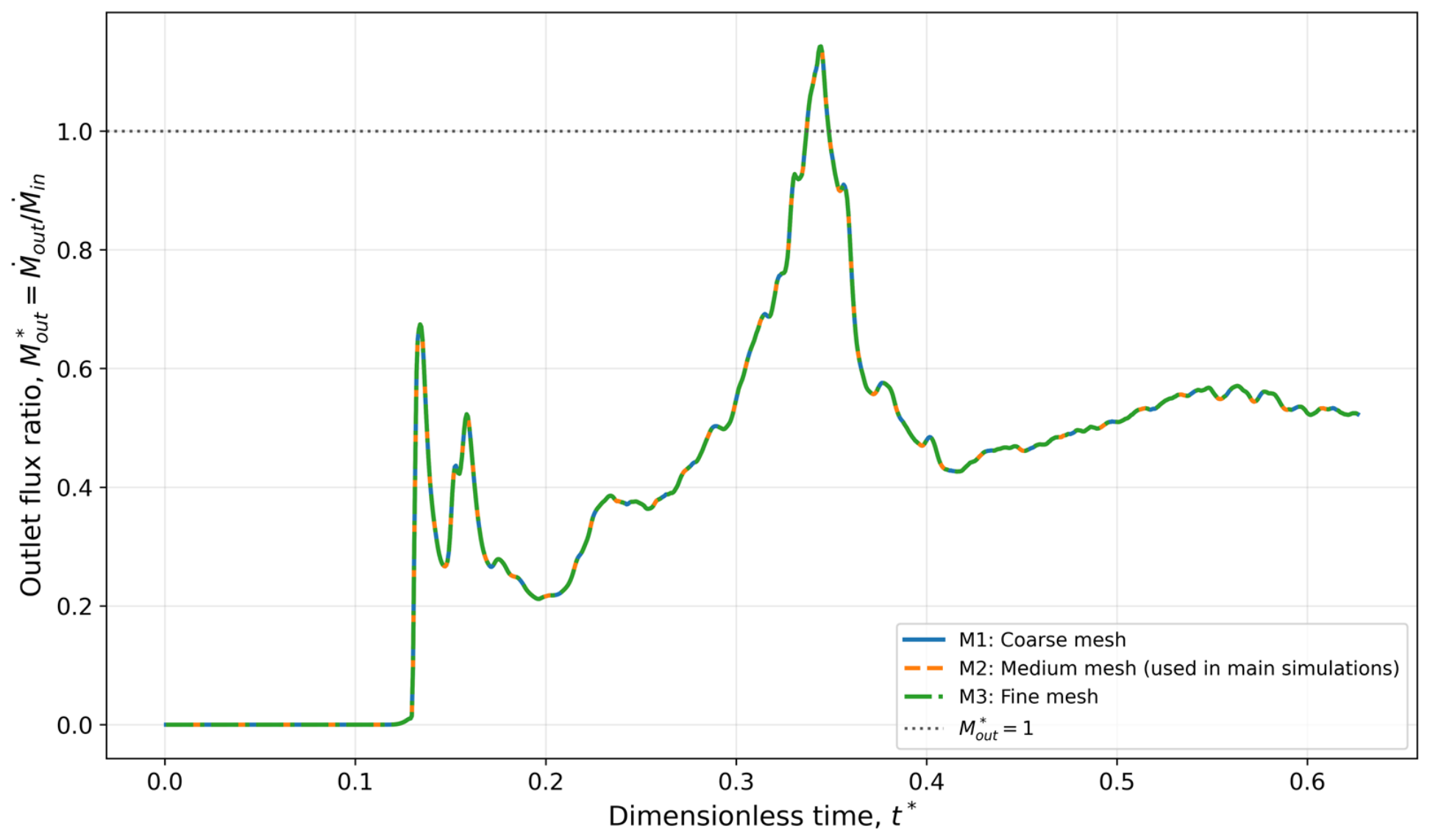
Appendix A.2. Vertical Profile Comparison
To supplement the scalar response comparison, vertical profiles of velocity magnitude and sediment mass concentration were compared at five streamwise sections: The vertical coordinate was defined relative to the local bed elevation as so that corresponded to the local bed at each section. At each height, the water region values were averaged in the lateral direction.
The vertical profile errors of M1 and M3 were additionally evaluated relative to that of M2. For velocity, the error was summarized using the mean absolute percentage error of . For sediment concentration, the error was evaluated in logarithmic space because varies over several orders of magnitude and approaches near-zero values in the upper water column:
where , is the number of vertical bins, and is a small positive value introduced to avoid the logarithm of zero. Figure A2 and Figure A3 show the vertical profiles of velocity magnitude and sediment mass concentration, respectively. Figure A4 summarizes the profile error metrics relative to M2. The fine mesh M3 was closer to M2 than the coarse mesh M1 for both the velocity and sediment concentration profiles. The velocity profile, of M3 remained approximately 4–7% across the five sections, whereas that of M1 showed larger deviations, particularly in the upstream sections. The sediment concentration increased downstream because the upper-column concentration became very small and the logarithmic comparison became more sensitive. Nevertheless, M3 showed lower concentration profile errors than M1 at all sections. These results, together with the negligible scalar sediment flux differences shown in Figure A1, support the use of the medium mesh M2 for the main simulations.
Figure A2.
Vertical profiles of velocity magnitude at , 200, 300, 400, and for the completed meshes.
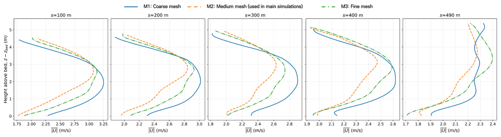
Figure A3.
Vertical profiles of sediment mass concentration at , 200, 300, 400, and for the completed meshes.
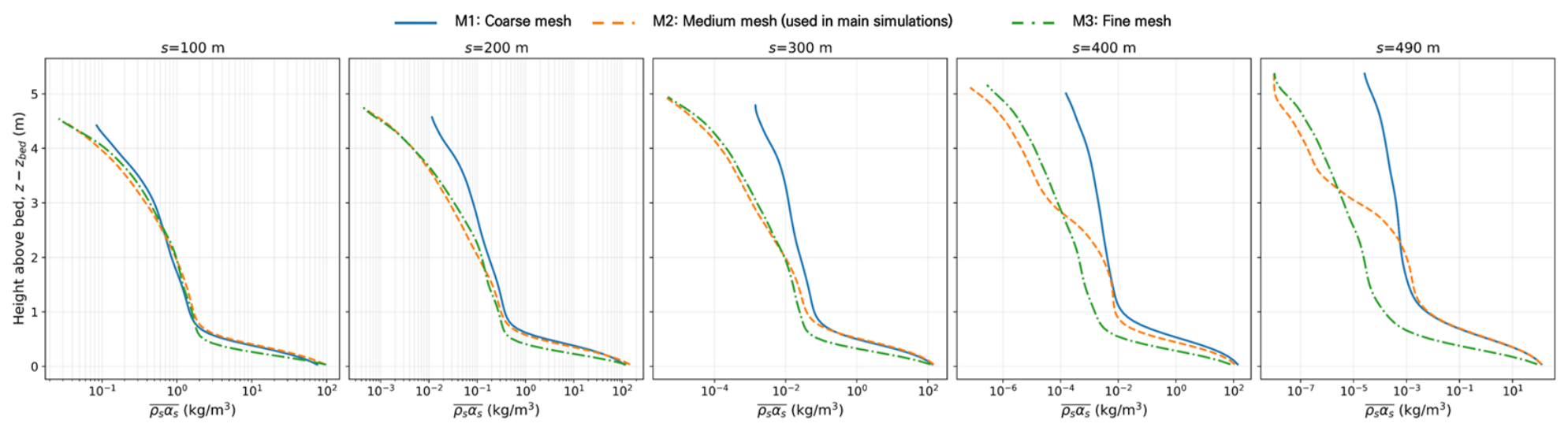
Figure A4.
Vertical profile error metrics relative to M2: (a) velocity profile and (b) sediment concentration profile .
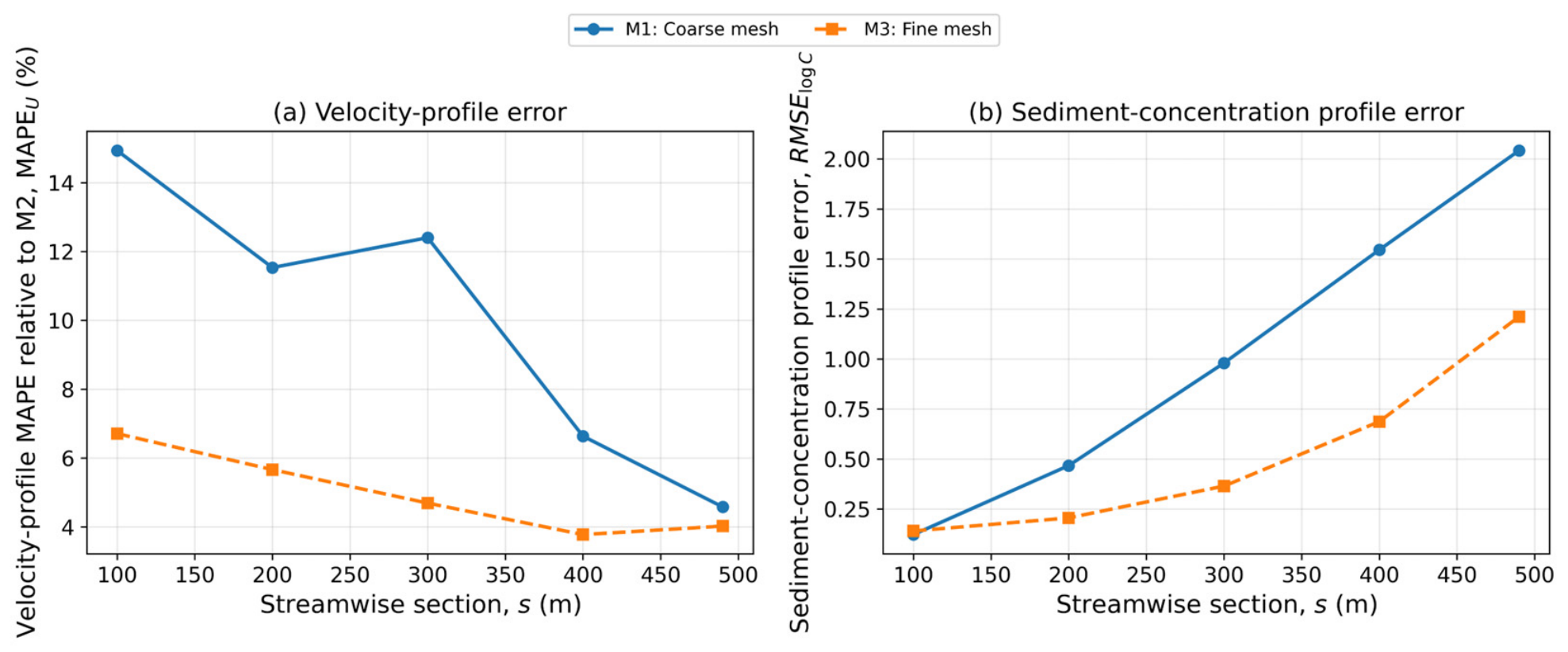
Appendix B
Reference Conditions and Regression Coefficients for the Proposed Dimensionless Deposition Formula
Appendix B provides the reference conditions and regression coefficients used in the proposed USLE-style dimensionless deposition formula. Table A2 summarizes the normalization basis used in Equations (43)–(45), while Table A3 reports the regression coefficients and error statistics associated with Equation (46).
Table A2.
Reference conditions and normalization basis used for the proposed dimensionless deposition formula.
Table A3.
Regression coefficients and error statistics of the proposed USLE-style dimensionless deposition formula.
Appendix C. Supplementary Field-Based Results for Concentration-Dependent Deposition
Longitudinal TKE and Distributions for Cases 1–8
Appendix C provides supplementary field-based results supporting the concentration-dependent deposition interpretation in Section 4.2.4. The main text presents the longitudinal sediment concentration distribution and the near-bed TKE-based diagnostic results directly needed for the interpretation, while Appendix C provides the corresponding longitudinal TKE and Rsus distributions for Cases 1–8, together with the field-based metrics summarized in Table A4.
Table A4.
Near-bed sediment retention and concentration-weighted turbulence metrics for the analysis reach –.
Figure A5.
Longitudinal TKE fields for Cases 1–8. The contours show the water-masked , with the local bed and free surface indicated by solid and dashed lines, respectively.
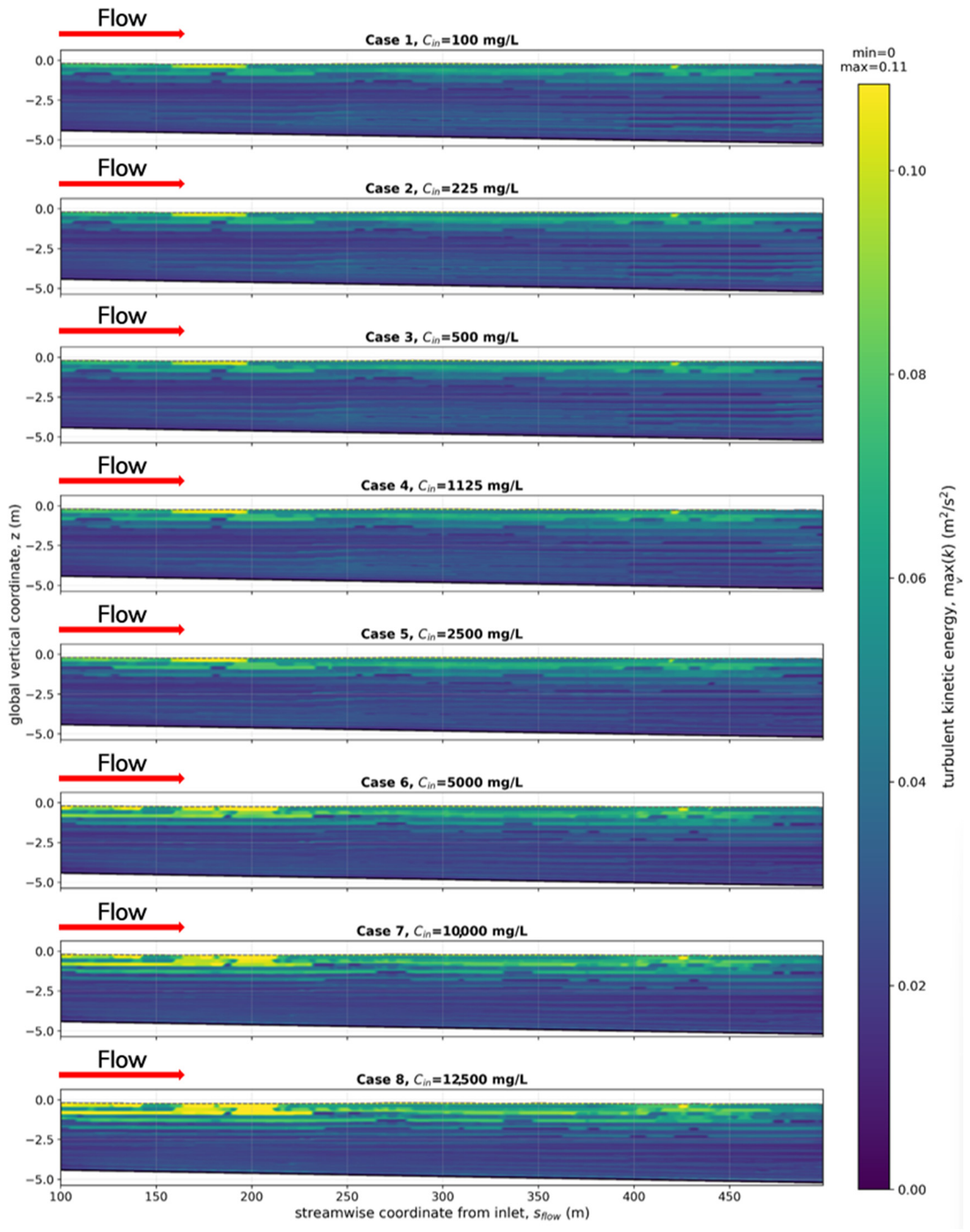
Figure A6.
Longitudinal fields for Cases 1–8. Contours show water-masked , where .
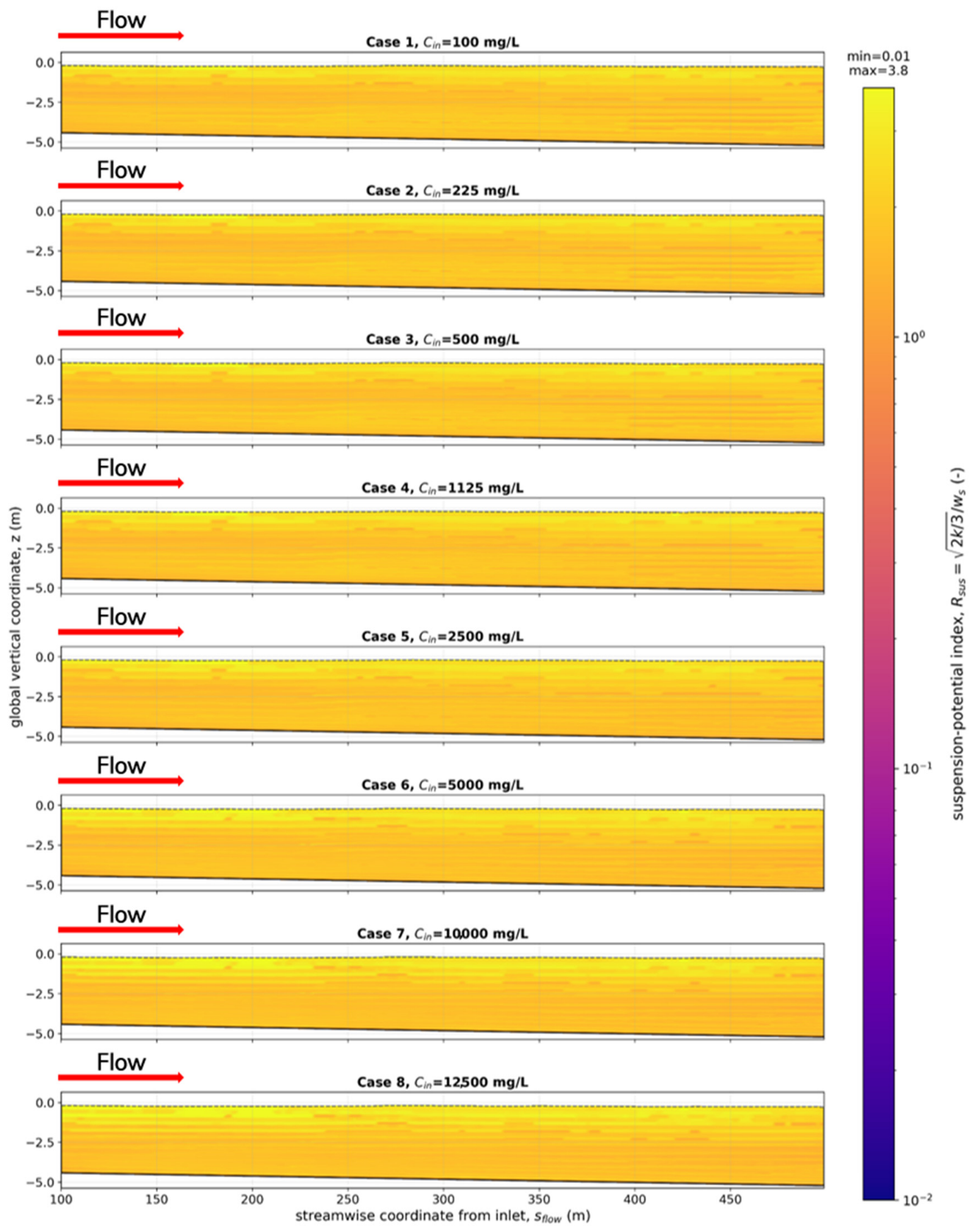
References
- Vasconcelos, J.G.; Wright, S.J. Anticipating Transient Problems during the Rapid Filling of Deep Stormwater Storage Tunnel Systems. J. Hydraul. Eng. 2017, 143, 06016025. [Google Scholar] [CrossRef] [Scilit]
- Hwang, S.H.; Kim, M.S.; Yoon, S.G.; Lee, Y.S. Improvement Plan for Multi-Purpose Utilization of Deep Underground Tunnels in Seoul; The Seoul Institute: Seoul, Republic of Korea, 2025. [Google Scholar]
- Yang, Z.; Huang, B.; Zhu, D.Z. Quantifying sediment deposition in sewers through hydraulic performance analysis. Water Sci. Technol. 2025, 91, 1058–1076. [Google Scholar] [CrossRef] [Scilit] [PubMed]
- Murali, M.; Hipsey, M.R.; Ghadouani, A.; Yuan, Z. SewerSedFoam: A Model for Free Surface Flow, Sediment Transport, and Deposited Bed Morphology in Sewers. Water 2020, 12, 270. [Google Scholar] [CrossRef] [Scilit]
- Alihosseini, M.; Sægrov, S.; Thamsen, P.U. CFD-DEM modelling of sediment transport in sewer systems under steady and unsteady flow conditions. Water Sci. Technol. 2020, 80, 2141–2147. [Google Scholar] [CrossRef] [Scilit]
- Alihosseini, M.; Thamsen, P.U. Numerical and Experimental Investigation of Flow in Partially Filled Sewer Pipes. Tech. Mech. 2019, 39, 113–124. [Google Scholar]
- Cho, Y.J. Optimal design of deep stormwater drainage tunnels to address urban flooding in Korea. Sci. Rep. 2024, 14, 24896. [Google Scholar] [CrossRef] [Scilit] [PubMed]
- Kim, S.Y.; Kim, J.S.; Yoon, S.E. Analysis of Discharge Capacity for Intake Structure at Deep Underground Storm Water Tunnel Using Fluent Model. J. Korean Soc. Hazard Mitig. 2014, 14, 255–262. (In Korean) [Google Scholar] [CrossRef] [Scilit]
- Park, S.; Kim, J.; Kang, J. Exploring optimal deep tunnel sewer systems to enhance urban pluvial flood resilience in the Gangnam region, South Korea. J. Environ. Manag. 2024, 357, 120762. [Google Scholar] [CrossRef] [Scilit] [PubMed]
- Montes, C.; Kapelan, Z.; Saldarriaga, J. Predicting non-deposition sediment transport in sewer pipes using Random forest. Water Res. 2021, 189, 116639. [Google Scholar] [CrossRef] [Scilit] [PubMed]
- Lee, J.H.; Cho, Y.J.; Bang, K.W. Characteristics of stormwater quality and particle-size distribution from urban roadways. J. Korean Soc. Environ. Eng. 2005, 27, 777–784. (In Korean) [Google Scholar]
- Kim, Y.I.; Kim, S.G.; Kang, S.W.; Yoon, S.L.; Kim, S.J. Stormwater pollutant characteristics from non-point source on urban roadway. J. Korean Soc. Environ. Eng. 2006, 28, 104–110. (In Korean) [Google Scholar]
- Lee, J.H.; Bang, K.W. Characterization of urban stormwater runoff. Water Res. 2000, 34, 1773–1780. [Google Scholar] [CrossRef] [Scilit]
- Coleman, N.L. Effects of suspended sediment on the open-channel velocity distribution. Water Resour. Res. 1986, 22, 1377–1384. [Google Scholar] [CrossRef] [Scilit]
- Meyer-Peter, E.; Müller, R. Formulas for Bed-Load Transport. In Proceedings of the 2nd Meeting of the International Association for Hydraulic Structures Research, Stockholm, Sweden, 7–9 June 1948; pp. 39–64. [Google Scholar]
- Yang, C.T. Incipient Motion and Sediment Transport. J. Hydraul. Div. 1973, 99, 1679–1704. [Google Scholar] [CrossRef] [Scilit]
- Shen, H.W.; Hung, C.S. An Engineering Approach to Total Bed Material Load by Regression Analysis. In Proceedings of the Sedimentation Symposium, Berkeley, CA, USA, 21–22 June 1971; pp. 14-1–14-17. [Google Scholar]
- Ackers, P.; White, W.R. Sediment Transport: New Approach and Analysis. J. Hydraul. Div. 1973, 99, 2041–2060. [Google Scholar] [CrossRef] [Scilit]
- Engelund, F.; Hansen, E. A Monograph on Sediment Transport in Alluvial Streams; Teknisk Forlag: Copenhagen, Denmark, 1967; 62p. [Google Scholar]
- Toffaleti, F.B. Definitive Computations of Sand Discharge in Rivers. J. Hydraul. Div. 1969, 95, 225–248. [Google Scholar] [CrossRef] [Scilit]
- Wischmeier, W.H.; Smith, D.D. Predicting Rainfall Erosion Losses—A Guide to Conservation Planning; USDA Agriculture Handbook 537; U.S. Government Printing Office: Washington, DC, USA, 1978.
- Mathieu, A.; Kim, Y.; Hsu, T.-J.; Bonamy, C.; Chauchat, J. sedInterFoam 1.0: A three-phase numerical model for sediment transport applications with free surfaces. Geosci. Model Dev. 2025, 18, 1561–1573. [Google Scholar] [CrossRef] [Scilit]
- Hirt, C.W.; Nichols, B.D. Volume of fluid (VOF) method for the dynamics of free boundaries. J. Comput. Phys. 1981, 39, 201–225. [Google Scholar] [CrossRef] [Scilit]
- Chauchat, J.; Cheng, Z.; Nagel, T.; Bonamy, C.; Hsu, T.-J. SedFoam-2.0: A 3-D two-phase flow numerical model for sediment transport. Geosci. Model Dev. 2017, 10, 4367–4392. [Google Scholar] [CrossRef] [Scilit]
- Lun, C.K.K.; Savage, S.B.; Jeffrey, D.J.; Chepurniy, N. Kinetic theories for granular flow: Inelastic particles in Couette flow and slightly inelastic particles in a general flow field. J. Fluid Mech. 1984, 140, 223–256. [Google Scholar] [CrossRef] [Scilit]
- Auton, B.J.; Hunt, J.C.R.; Prud’homme, M. The force exerted on a body in inviscid unsteady non-uniform rotational flow. J. Fluid Mech. 1988, 197, 241–257. [Google Scholar] [CrossRef] [Scilit]
- Colby, B.R.; Hembree, C.H. Computations of Total Sediment Discharge, Niobrara River near Cody, Nebraska; U.S. Geological Survey Water-Supply Paper 1357; U.S. Government Printing Office: Washington, DC, USA, 1955; 187p. [CrossRef] [Scilit]
- Einstein, H.A. The Bed-Load Function for Sediment Transportation in Open Channel Flows; USDA Soil Conservation Service, Technical Bulletin No. 1026; U.S. Government Printing Office: Washington, DC, USA, 1950; 71p.
- Laursen, E.M. The Total Sediment Load of Streams. J. Hydraul. Div. 1958, 84, 1–36. [Google Scholar] [CrossRef] [Scilit]
- Hubbell, D.W.; Matejka, D.Q. Investigations of Sediment Transportation, Middle Loup River at Dunning, Nebraska: With Application of Data from Turbulence Flume; U.S. Geological Survey Water-Supply Paper 1476; U.S. Government Printing Office: Washington, DC, USA, 1959; 123p. [CrossRef] [Scilit]
- Jordan, P.R. Fluvial Sediment of the Mississippi River at St. Louis, Missouri; U.S. Geological Survey Water-Supply Paper 1802; U.S. Government Printing Office: Washington, DC, USA, 1965; 89p. [CrossRef] [Scilit]
- Nordin, C.F. Aspects of Flow Resistance and Sediment Transport, Rio Grande near Bernalillo, New Mexico; U.S. Geological Survey Water-Supply Paper 1498-H; U.S. Government Printing Office: Washington, DC, USA, 1964; 41p.
- Yang, C.T.; Stall, J.B. Applicability of Unit Stream Power Equation. J. Hydraul. Div. 1976, 102, 559–568. [Google Scholar] [CrossRef] [Scilit]
- ASCE Task Committee on Relations Between Morphology of Small Streams and Sediment Yield of the Committee on Sedimentation of the Hydraulics Division. Relationships between morphology of small streams and sediment yield. J. Hydraul. Div. 1982, 108, 1328–1365.
- Alonso, C.V.; Neibling, W.H.; Foster, G.R. Estimating sediment transport capacity in watershed modeling. Trans. ASAE 1981, 24, 1211–1220. [Google Scholar] [CrossRef] [Scilit]
- Yang, C.T.; Wan, S. Comparisons of Selected Bed-Material Load Formulas. J. Hydraul. Eng. 1991, 117, 973–989. [Google Scholar]
- Einstein, H.A.; Chien, N. Transport of Sediment Mixtures with Large Ranges of Grain Sizes; M.R.D. Sediment Series Report No. 2; U.S. Army Corps of Engineers, Missouri River Division: Omaha, NE, USA, 1953.
- Lee, D.S. Understanding of Deep Stormwater Drainage Tunnels (Underground Floodwater Conduits). In Proceedings of the 2nd Discussion Forum of the Water Resources Issues Committee, Korea Water Resources Association (KWRA), Seoul, Republic of Korea, 27 June 2023; Available online: https://www.kwra.or.kr/media/staticdata_uploads/2023/06/27/2-_.pdf (accessed on 8 June 2026). (In Korean)
- Park, S.H.; Oh, J.O.; Park, J.H.; Park, C.K. A study on the inflow characteristics according to design conditions of vertical inlet of Sinwol rainwater storage and drainage facility. J. Korea Water Resour. Assoc. 2017, 50, 99–108. (In Korean) [Google Scholar]
- Seoul Metropolitan Government, Urban Infrastructure Headquarters. Operation Manual of the Sinwol Rainwater Storage and Drainage Facility; Seoul Metropolitan Government: Seoul, Republic of Korea, 2020. (In Korean)
- Lee, Y.S.; Jeong, C.J.; Seo, G.W.; Lee, S.O. Suggestion for the sediment classification system for underground stormwater tunnels. In Proceedings of the 2025 KSMI Conference, Daejeon, Republic of Korea, 18 April 2025. [Google Scholar]
- Winterwerp, J.C. On the flocculation and settling velocity of estuarine mud. Cont. Shelf Res. 2002, 22, 1339–1360. [Google Scholar] [CrossRef] [Scilit]
- Cellino, M.; Graf, W.H. Sediment-laden flow in open-channels under noncapacity and capacity conditions. J. Hydraul. Eng. 1999, 125, 455–462. [Google Scholar]
- Brune, G.M. Trap Efficiency of Reservoirs. Trans. Am. Geophys. Union 1953, 34, 407–418. [Google Scholar] [CrossRef] [Scilit]
- Roache, P.J. Quantification of Uncertainty in Computational Fluid Dynamics. Annu. Rev. Fluid Mech. 1997, 29, 123–160. [Google Scholar] [CrossRef] [Scilit]
- Celik, I.B.; Ghia, U.; Roache, P.J.; Freitas, C.J.; Coleman, H.; Raad, P.E. Procedure for Estimation and Reporting of Uncertainty Due to Discretization in CFD Applications. J. Fluids Eng. 2008, 130, 078001. [Google Scholar] [CrossRef] [Scilit]
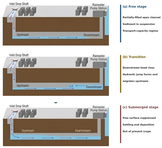
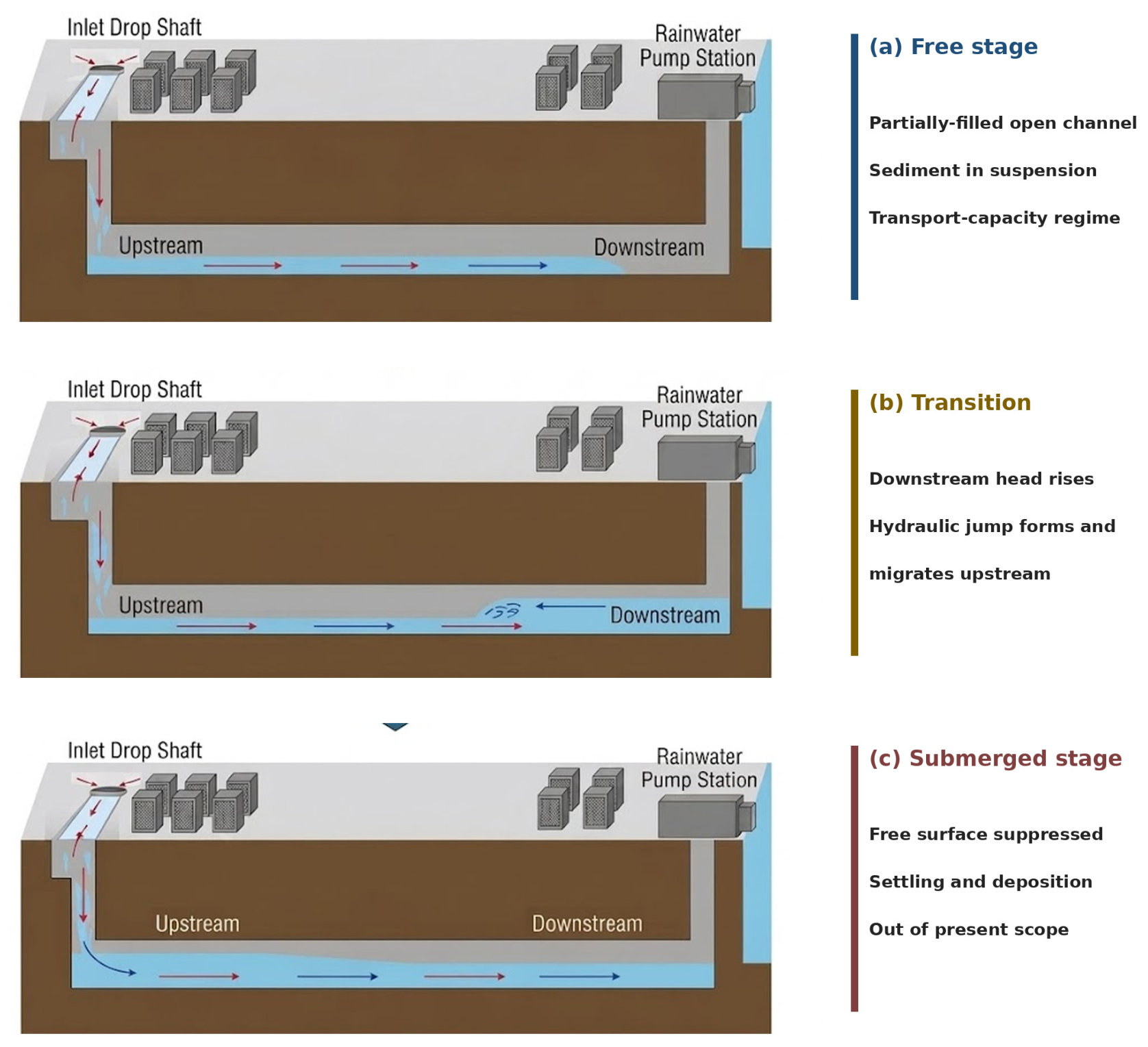


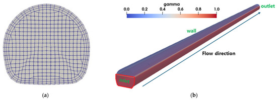
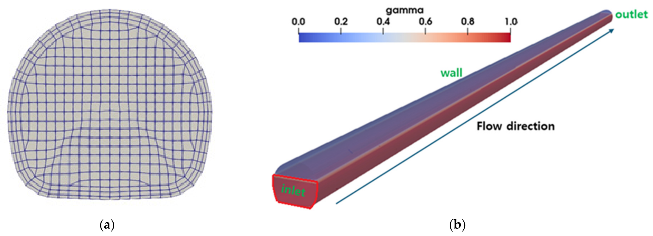
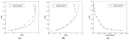
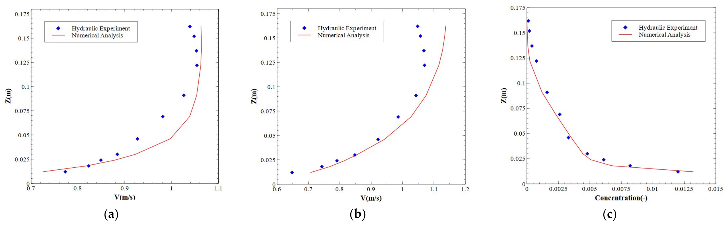
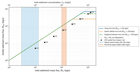
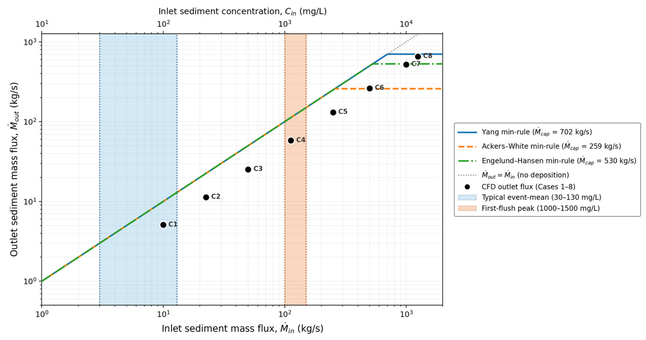
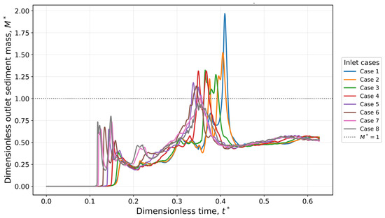
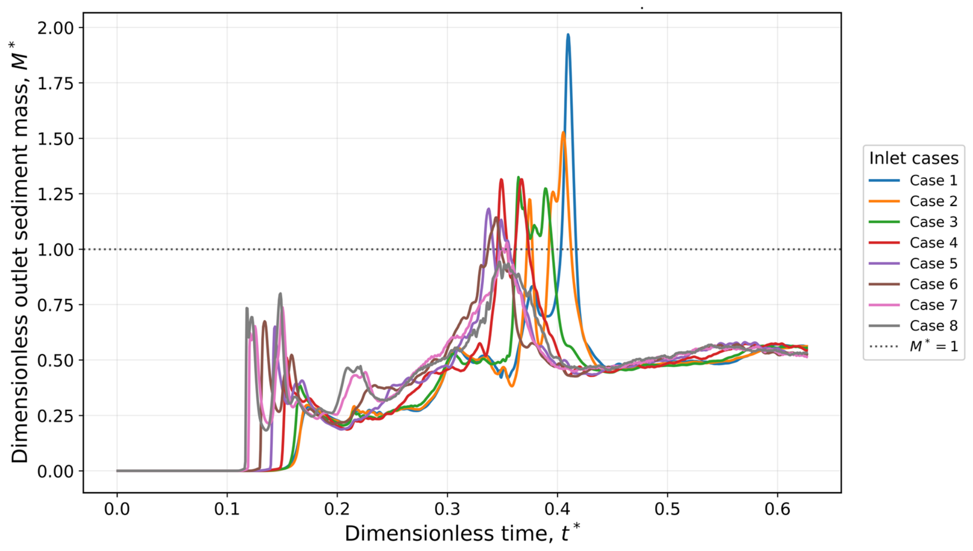
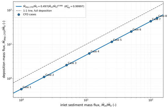
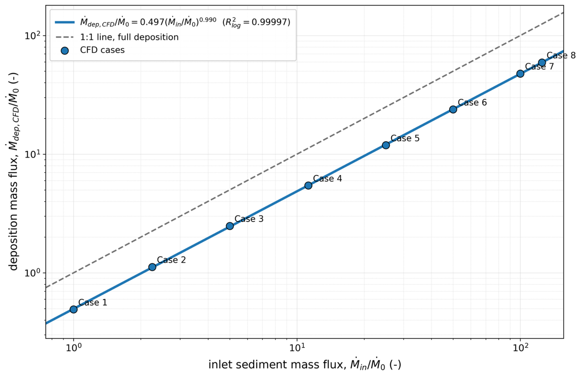
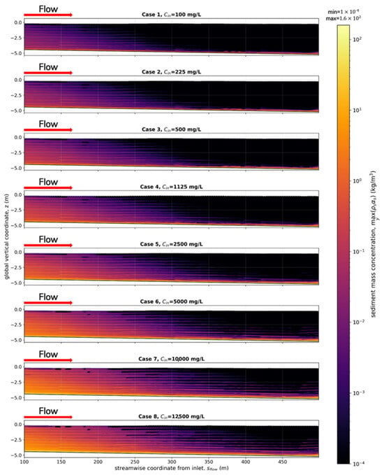
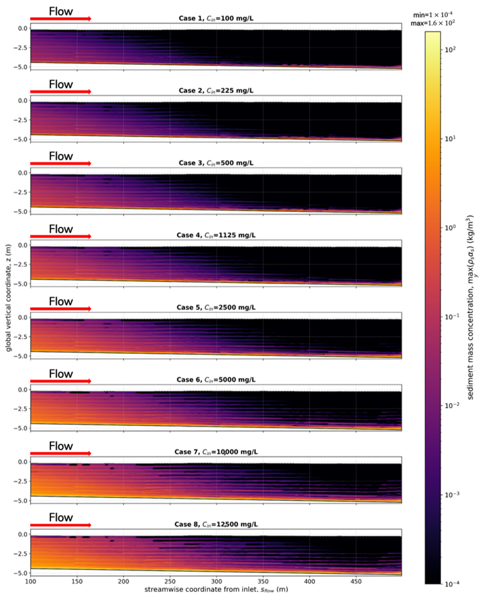
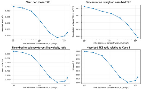
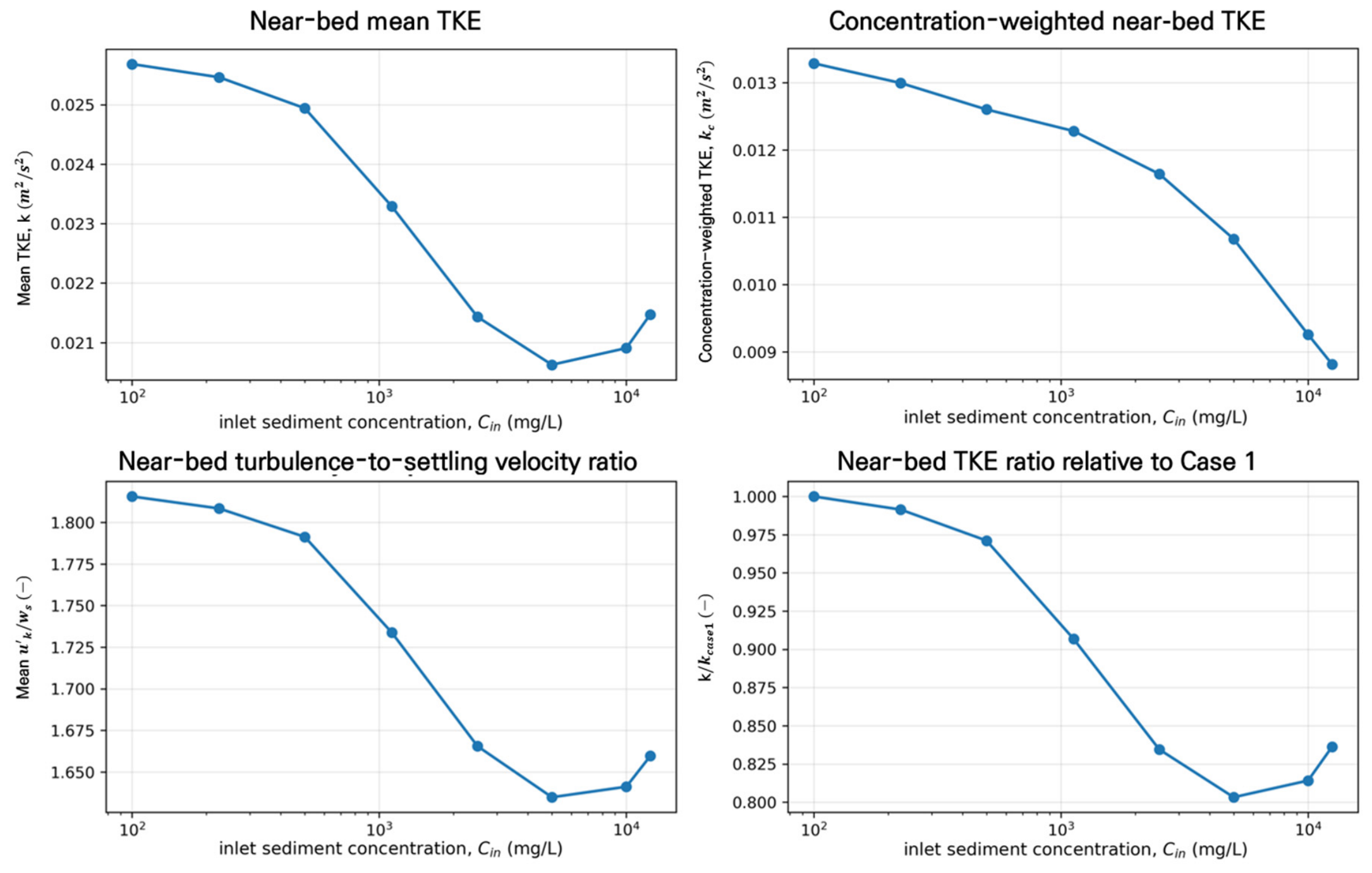

Disclaimer/Publisher’s Note: The statements, opinions and data contained in all publications are solely those of the individual author(s) and contributor(s) and not of MDPI and/or the editor(s). MDPI and/or the editor(s) disclaim responsibility for any injury to people or property resulting from any ideas, methods, instructions or products referred to in the content. |
© 2026 by the authors. Licensee MDPI, Basel, Switzerland. This article is an open access article distributed under the terms and conditions of the Creative Commons Attribution (CC BY) license.