


Abstract
This study investigates the spatiotemporal dynamics and driving mechanisms of Water Supply Ecosystem Service Value (ESV) in the North China Plain from 2002 to 2022. Addressing the critical challenges of water scarcity and ecological degradation in this densely populated and agriculturally intensive region, the research develops an integrated framework to quantify the relative contributions of multi-dimensional drivers to the water supply service (quantified by biophysical supply, W). A Particle Swarm Optimization (PSO) algorithm was employed to automate hyperparameter tuning for XGBoost and Random Forest models, with model interpretability enhanced via SHAP (SHapley Additive exPlanations) to elucidate non-linear feature importance and directional impacts. Results demonstrate that the PSO-XGBoost model outperforms PSO-Random Forest in predictive performance (R2 = 0.8013 vs. 0.7443). The total water supply exhibited a significant annual decline of 1.98 billion m3 (p < 0.05), with 53.4% of the study area showing significant pixel-level temporal trends. The supply structure is dominated by soil moisture (80–90%), while externally transferred water, despite increasing rapidly, exhibits high interannual variability. SHAP analysis identifies vegetation cover (NDVI), clay content, GDP, and population density as the predominant drivers. Notably, GDP shows a strong negative correlation with water supply, reflecting a trade-off where intensive socio-economic expansion increases water consumption at the expense of ecosystem supply capacity. Methodologically, the PSO-XGBoost-SHAP framework enables both high predictive accuracy and detailed attribution of driving factors. These findings highlight the strategic importance of soil water (“Green Water”) conservation and offer actionable insights for adaptive water resource management, providing a replicable analytical approach for other regions facing similar hydrological challenges.
1. Introduction
Recent studies have highlighted the importance of ecosystem service value (ESV) assessment in the field of water resource management, particularly for water-scarce regions facing severe ecological degradation [1,2]. In the North China Plain, the escalating prevalence of groundwater overexploitation and surface water depletion has intensified concerns regarding regional water security and sustainable development [3,4]. Consequently, understanding the dynamics of water supply has become essential, as these processes are shaped by complex interactions between natural hydrological cycles and intensive human interventions [5]. However, accurately quantifying these spatiotemporal dynamics remains challenging. Current evaluative frameworks often lack the capacity to integrate multi-dimensional drivers—such as climatic, topographic, and anthropogenic factors—and fail to capture their non-linear interactions [6,7]. Furthermore, the neglect of regional heterogeneity within these oversimplified models restricts their effectiveness in informing targeted and adaptive water management policies [8].
Despite its importance, the complex interplay between natural climate variability and intensive human activities in shaping water supply remains poorly understood, particularly through the lens of spatial heterogeneity and temporal evolution. The inherent non-linearity of these drivers poses a significant challenge for traditional analytical models. Consequently, the lack of research leveraging advanced machine learning coupled with explainable AI (e.g., SHAP) represents a major bottleneck. Without such interpretable frameworks, it is difficult to move beyond descriptive analysis toward the development of precise, evidence-based water management strategies [9].
This study aims to unravel the spatiotemporal dynamics of water supply ESV in the North China Plain from 2002 to 2022 by quantifying the relative importance of multi-dimensional drivers through an integrated PSO-XGBoost-SHAP analytical framework. Specifically, it investigates the non-linear interactions among climatic variables (precipitation, temperature, PET), topographic factors (DEM, slope, AWC), vegetation indicators (NDVI), and anthropogenic metrics (population density, GDP) to identify dominant control mechanisms and their spatial variations. By integrating pixel-level trend analysis with interpretable machine learning, this research provides a granular understanding of water resource drivers in this critical agricultural and population hub.
By disentangling the differential impacts of natural and anthropogenic drivers, this study fills a crucial gap in regional ESV research and advances our understanding of human-water-ecosystem interactions under intensive pressure, ultimately supporting the sustainability of vital ecosystem services.
The main contributions of this study are summarized as follows: (1) Integrated Assessment Framework: We developed a pixel-level framework that couples biophysical water supply modeling with dynamic value assessment, overcoming the limitations of traditional administrative-scale or static LULC-based evaluations. (2) Interpretable Machine Learning Approach: By introducing the PSO-XGBoost-SHAP framework, we successfully captured the complex non-linear interactions and threshold effects of multi-dimensional drivers, providing a more granular understanding of water supply dynamics. (3) Long-term Spatiotemporal Insight: This research quantifies the 20-year evolution of water supply ESV in the North China Plain, identifying critical degradation “hotspots” and the shifting dominance between natural climate variability and anthropogenic interventions.
2. Overview of the Study Area and Data Sources
2.1. Overview of the Research Area
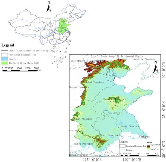
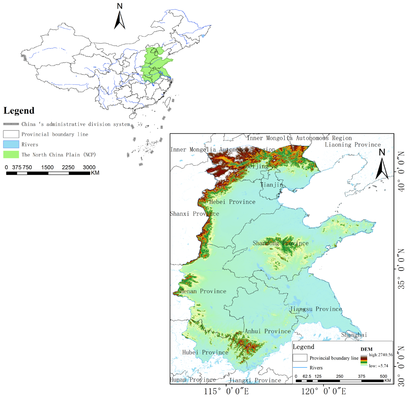
The North China Plain (Figure 1) is located in eastern China, situated in the lower reaches of the Yellow River, Huai River, and Hai River, with a total area of approximately 300,000 square kilometers. The North China Plain encompasses the vast majority of the Hai River Basin as well as parts of the Yellow River Basin and Huai River Basin [10]. In water resources management and valuation, the Hai River Basin is the core component of the water resources system of the North China Plain. The region is characterized by flat and gentle terrain, with plains accounting for more than 95% of the area [11]. From west to east, it consists of alluvial tilted plains, alluvial plains, and coastal plains, with elevations mostly between 5–100 m. It falls under a temperate monsoon climate, with annual precipitation of 500–800 mm (only 60–80% of the national average), 70% of which occurs in summer (June to August), and with significant interannual variability (the ratio of wet to dry years can reach 3–5 times); potential evapotranspiration ranges from 800–1200 mm, far exceeding precipitation, forming a water deficit hydrological pattern. The total natural water resources are about 50 billion cubic meters, accounting for only 1.5% of the national total, with per capita water resources of less than 300 cubic meters (one-seventh of the national average of 2100 cubic meters, far below the international “extreme water scarcity” threshold of 500 cubic meters), comparable to the levels of desert countries in the Middle East. The main rivers in the region (Hai River, Yellow River, Huai River) have low runoff and uneven seasonal distribution. The utilization rate of surface water has exceeded 80%, with long-term reliance on groundwater (accounting for more than 60% of total water supply), forming a “shallow-deep” composite over-extraction system [12].
Figure 1.
Overview of the Research Area (North China Plain).
As the nation’s main grain-producing region (with a cultivated land area of approximately 350 million mu, accounting for 23% of the country) and a densely populated area (hosting about 350 million people, or 18% of the national population), the water demand of the North China Plain far exceeds its ecological carrying capacity. Agricultural irrigation accounts for 70% of total water usage (mainly through flood irrigation, with an efficiency of less than 50%), while industrial (such as steel and chemical industries) and domestic water use account for 30%. Additionally, the urbanization rate has risen from 35% in 2000 to 65% in 2020, further intensifying water scarcity. Over the past 40 years, groundwater over-extraction has cumulatively exceeded 180 billion cubic meters, forming the 180,000 km2 “North China Funnel” (accounting for 60% of the plain’s area), leading to surface water shrinkage (for instance, the area of Baiyangdian Lake decreased from 560 km2 in 1950 to 250 km2 in 2020, a reduction of 55%), wetland ESV loss exceeding 60%, land subsidence (with the maximum in Tianjin exceeding 3 m), and soil salinization (covering 12,000 km2), among other cascading ecological problems [13].
2.2. Data Sources
The data for this study encompass water resource supply data, topographical factors, climatic factors, and human activity factors (Table 1). Climatic and topographical factors include annual average temperature (Avg. Temp), annual average precipitation (Precip.), potential evapotranspiration (ET0), normalized difference vegetation index (NDVI), field capacity to wilting point ratio (FC-WP), digital elevation model (DEM), and slope data. Regarding human activity factors, indicators such as population density and GDP were considered.
Table 1.
Factor and data sources (500 m resolution).
The data for Pvalue (Yuan/m3) and the adjustment coefficient K in Table 2 are sourced from the “China Water Resources Bulletin” published by the Ministry of Water Resources of the People’s Republic of China. This bulletin, compiled by the national authoritative department as an annual report on water resources, systematically records core data on the status of water resources and their development and utilization across the country and in each provincial-level administrative region, including key indicators such as precipitation, surface and groundwater resources, total water resources, water supply, water usage, and water use efficiency. The data collection strictly follows the national water use statistical survey standards and is jointly compiled and calculated by the Ministry of Water Resources together with watershed management agencies, provincial water authorities, and research institutions. It possesses a high degree of scientific accuracy and authority, providing reliable official data support for water resource management, policy-making, and academic research.
Table 2.
Data Source (Water Resources Bulletin of the People’s Republic of China).
3. Research Methods and Framework
3.1. ESV Estimation
ESV assessment is a fundamental approach for quantifying the benefits that ecosystems provide to humans. Among these services, water supply, as a key provisioning service, plays a crucial role in evaluating regional water resource management and informing ecological compensation policies. In ESV assessments, the main driving factors are typically categorized into two dimensions: biophysical and anthropogenic. These factors directly influence the hydrological processes of “precipitation–evapotranspiration–infiltration–runoff,” thereby shaping the spatiotemporal dynamics of regional water supply capacity.
The concept of water resource assets represents a shift from viewing water solely as a utilizable resource to recognizing its multifaceted value within both natural ecosystems and socio-economic systems. According to the hydrological cycle, water evaporates and condenses to form precipitation. A portion enters rivers, lakes, and reservoirs to become available for human use, while the remainder contributes to surface water flows. Surface water regulates infiltration into the soil, interacts with groundwater, and generates runoff, ultimately returning to the atmosphere through evaporation and plant transpiration, completing a cyclical process. Within the economic system, water resources exhibit ‘asset’ value through their allocation and use, reflecting significant economic attributes.
The ESV of water supply services essentially represents the economic value of the dynamically available water resources provided by the ecosystem. It can be calculated using the following formula:
In this formula, ESVw denotes the ecosystem service value of water supply (yuan per year); W represents the water supply quantity (dynamically available total volume, m3/year); P is the unit value of water supply (yuan/m3); and K is a regional correction factor (dimensionless), which accounts for natural and economic variations.
Specifically, the water supply W consists of several components:
Here, W denotes the total water resource supply; Wsa represents available surface water, Wge denotes exploitable groundwater, Wse indicates effective soil water, and Wo refers to externally transferred, recycled, or other sources of water. Units are typically expressed in m3/year or 108 m3/year; the total volume is used for regional assessments, while m3/(ha·year) is used for per-unit-area evaluations.
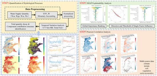
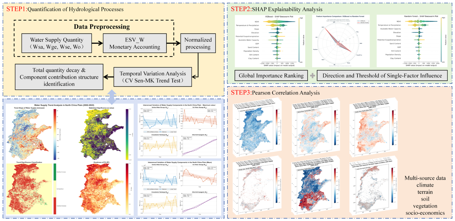
The technical framework is shown in Figure 2.
Figure 2.
Technical Flowchart.
This study constructs a technical framework of ‘multi-source data–process quantification–driver analysis–management application’: based on multi-source data including climate, topography, soil, vegetation, and socioeconomics, it quantifies water supply components (Wsa/Wge/Wse/Wo) and monetarily accounts for ESV-W. Through temporal variation analysis (CV Sen-MK), it identifies total decline and component contributions; by optimizing XGBoost modeling with PSO, combined with SHAP interpretability and spatial correlation mapping, it reveals the heterogeneity of driving forces, ultimately proposing adaptive management recommendations.
3.2. Calculation of CV Coefficient of Variation
Introducing the coefficient of variation (CV) in the ESV assessment of water resource supply services can quantify the temporal and spatial variability (degree of dispersion) of driving factors, identify key factors that are more ‘unstable’ in their impact on ESV, and provide a basis for risk assessment and refined management [14].
- Time Series CV (Interannual Coefficient of Variation)
For factors with significant interannual variation (such as precipitation, temperature, NDVI, and external water diversion), calculate the CV of the 2002–2022 series to assess their interannual volatility.
Among them, -interannual: interannual standard deviation; -interannual: interannual mean.
- 2.
- Spatial Distribution CV (Coefficient of Variation within a Region)
For factors with significant spatial heterogeneity (such as DEM, slope, and soil effective moisture content), calculate the CV within the study area to assess the unevenness of their spatial distribution.
Among them, the space: the standard deviation of pixel values within the study area; the space: the mean of pixel values within the study area.
3.3. Sen’s MK Trend Analysis
Sen’s MK trend analysis is a combination of Sen’s slope estimator and the Mann–Kendall (MK) non-parametric test, used to quantitatively describe the monotonic trend (increasing/decreasing) of a time series and to determine the statistical significance of the trend [15]. Because it does not rely on the assumption of normally distributed data and is resistant to outlier interference, it is widely applied in long-term time series analysis in fields such as climatology, hydrology, and ecology (e.g., precipitation, runoff, temperature, and changes in water resource supply).
- Sen’s Slope Estimation (Quantifying the Magnitude of Trends)
Consider a time series , , …, , where n is the sample size. For all pairs of data (, ) with i < j, the slope is computed as:
Sen’s slope , is defined as the median of all values:
Here, denotes the k-th value after all values have been sorted in ascending order. The interpretation of β is as follows:
β > 0: upward trend; β < 0: downward trend; β = 0: no trend.
- 2.
- Mann–Kendall Test (Determine Trend Significance)
Determining whether a trend is significant through statistical testing (excluding the impact of random fluctuations) primarily involves calculating the S statistic and the Z value (standardized statistic).
Construct the sign function: for i < j, define
Calculate the S statistic (sum of signs for all data pairs).
Standardized to Z-score (eliminating the effect of sample size)
The significance of a trend is assessed using the test statistic Z at a predetermined significance level α. In this study, α is set to 0.05, corresponding to a critical value of under the standard normal distribution. A time series trend is considered statistically significant if |Z| ≥ 1.96; otherwise, it is not significant. Furthermore, a positive Z indicates a significant upward trend, while a negative Z indicates a significant downward trend.
By constructing a cross-classification matrix of Sen’s slope (rate of change) and the Mann–Kendall test (statistical significance), the dynamic evolution of water resource supply in the study area is categorized into nine levels (Table 3). Specifically, when the absolute value of Sen’s slope is greater than or equal to 0.1, further subdivisions into moderate, significant, and extreme changes are determined based on the MK test results (p < 0.05 indicates significance, 0.05 ≤ p < 0.1 indicates marginal significance). When Sen’s slope lies between −0.1 and 0.1, the trend is considered stable (including slight increases or decreases), regardless of statistical significance. This classification system enables a two-dimensional, precise identification of hydrological sequence trends in terms of “magnitude-confidence,” providing a quantitative basis for subsequent spatiotemporal pattern analysis.
Table 3.
Trend Categories of Sen-MK Test.
3.4. Driving Mechanism Analysis Framework Based on PSO-Optimized Machine Learning and SHAP
To investigate the driving mechanisms underlying ESVW, this study adopts an integrated framework coupling ensemble machine learning with explainable artificial intelligence (XAI). By quantifying the contributions of diverse environmental and socioeconomic factors, we aim to pinpoint the primary determinants influencing water supply variations. In the valuation model, since the price factor (P) and the social developmental stage coefficient (K) remain constant across the study area or are fixed for specific years, the driving analysis conducted on the physical water supply (W) is mathematically equivalent to the analysis of the spatial heterogeneity of ESVW. This methodological alignment allows for a focused investigation into the biophysical and anthropogenic drivers that fundamentally govern the provisioning and valuation of this ecosystem service.
- Principles of the Particle Swarm Optimization Algorithm
The Particle Swarm Optimization (PSO) algorithm, proposed by Kennedy and Eberhart in 1995, is a swarm intelligence optimization algorithm inspired by the foraging behavior of birds [16,17]. This algorithm simulates the collective cooperative behavior found in nature and searches for the global optimal solution in the solution space through information sharing and experience transmission among individuals. The PSO algorithm has the advantages of a simple structure, fast convergence speed, and few parameters, and it has been widely applied in function optimization, machine learning, engineering design, and other fields.
In the PSO algorithm, each potential solution is regarded as a ‘particle’ in the search space. Let the search space be D-dimensional, and the position vector and velocity vector of the i-th particle at time t are represented as:
The Particle Swarm Optimization (PSO) algorithm was employed to determine the optimal hyperparameters for the machine learning models. In this heuristic search process, each particle i represents a potential solution set in the d-dimensional parameter space, characterized by its position and velocity. The velocity and position of each particle are updated iteratively according to Equations (11) and (12):
where ω denotes the inertia weight, which controls the influence of the particle’s previous velocity. and represent the cognitive and social learning factors, respectively. r1 and r2 are random numbers uniformly distributed within the interval [0,1]. denotes the personal best position of particle i, while represents the global best position of the swarm. d = 1, 2, …, D indicates the dimensional index.
To ensure algorithm stability, particle velocity is usually subject to the following constraints:
Here, is the maximum velocity in the d-th dimension, usually set to 20% of the search range in that dimension.
- 2.
- X-G BOOST Regression Analysis Based on Particle Swarm Optimization Algorithm
To address the nonlinear, high-dimensional characteristics and hyperparameter sensitivity in water resource supply forecasting, this study proposes a regression framework that integrates Particle Swarm Optimization (PSO) with Extreme Gradient Boosting (XGBoost), hereafter referred to as PSO-XGBoost. This framework leverages the global search capability of PSO to automatically optimize the hyperparameters of XGBoost, with the objective of minimizing prediction errors and improving model accuracy. It further supports robust modeling and mechanism analysis of water resource supply.
The main advantages of this approach include automated hyperparameter tuning (eliminating manual trial-and-error), strong nonlinear fitting capability based on the XGBoost gradient boosting framework, and efficient global optimization enabled by the swarm intelligence mechanism of PSO.
XGBoost is an ensemble learning algorithm based on Gradient Boosting Decision Trees (GBDT). It constructs an additive model by integrating multiple weak learners (CART regression trees) and incorporates regularization terms to control model complexity and prevent overfitting. The core principle is described as follows.
Let the training set be denoted as , where represents the feature vector and denotes the observed value of water resource supply. The XGBoost prediction model can then be expressed as an ensemble of K regression trees:
where: denotes the predicted value of the i-th sample, fk represents the k-th regression tree, xi is the input feature vector, and K is the total number of trees.
The objective function of XGBoost consists of two components: a loss function and a regularization term.
where denotes the loss function that measures the discrepancy between the observed and predicted values, and represents the regularization term that controls model complexity.
The complexity of an individual tree, , is defined as follows:
where T denotes the number of leaf nodes, represents the weight of the j-th leaf node, and γ and λ are regularization parameters.
XGBoost employs a forward stagewise additive algorithm. At the t-th iteration, the objective is to determine an optimal tree that minimizes the following objective function:
where and denote the first- and second-order derivatives (gradients) of the loss function, respectively.
Among these,
For a given tree structure q, the optimal weight of the j-th leaf node, denoted as , and the corresponding objective function value (i.e., the structure score) are given by:
where denotes the set of samples assigned to the j-th leaf node.
The splitting gain, denoted as , is used to determine the optimal splitting feature and corresponding threshold:
where and denote the sums of the first-order gradients of the left and right child nodes, respectively, while and represent the corresponding sums of the second-order gradients. The split that yields the maximum gain is selected as the optimal partition.
- 3.
- Random Forest Regression Analysis Based on Particle Swarm Optimization Algorithm
XGBoost is a powerful gradient-boosted decision tree (GBDT) framework designed for speed and performance [18,19]. Unlike traditional boosting methods, XGBoost implements a Taylor expansion of the loss function to improve computational efficiency and incorporates a regularization term to control model complexity and prevent overfitting. The objective function is expressed as:
where l is the loss function measuring the difference between the prediction and the target . The regularization term is defined as:
where T represents the number of leaves in the tree and is the norm of the leaf weights. To maximize the predictive performance of XGBoost, Particle Swarm Optimization (PSO) was employed to automate hyperparameter tuning. The iterative update of the swarm followed the velocity and position mechanisms previously described in Equations (11) and (12). The primary hyperparameters optimized included the learning rate, maximum tree depth, number of estimators, subsample ratio, and regularization parameters ( and ). This integration ensures that the XGBoost model achieves optimal generalizability for mapping water supply dynamics across the North China Plain.
- 4.
- Variable Importance Analysis Based on the SHAP Algorithm
In this study, the SHAP (SHapley Additive exPlanations) algorithm was used to analyze variable importance in the random forest model to assess the impact of various driving factors on changes in farmland use efficiency [20,21]. SHAP (SHapley Additive exPlanations) is a game theory-based model interpretation method that quantifies each driving factor’s ‘responsibility share’ for the outcome by calculating its marginal contribution (Shapley value) to the target variable (e.g., water resource supply W). The core idea is to treat the model prediction as a ‘team effort,’ where the contribution of each factor (feature) equals its ‘average marginal gain’ across all possible combinations of factors.
For the target variable y (water resource supply) and the driving factors (such as precipitation and groundwater extraction), the SHAP value satisfies:
Here, is the baseline value (the predicted result when all factors take their mean values), and is the SHAP value of factor . A positive indicates that the factor promotes an increase in y, while < 0 indicates that it inhibits the increase in y. The larger the absolute value, the stronger the contribution.
3.5. Statistical Metrics for Model Validation
To evaluate the predictive performance of the machine learning models (RF, XGBoost, and PSO-XGBoost) in simulating the Drivers of the Water Supply Service (represented by W), three statistical metrics were employed: the coefficient of determination (R2), Root Mean Square Error (RMSE), and Mean Absolute Error (MAE). The formulas for these metrics are as follows:
where n is the total number of samples, is the actual observed value for the i-th sample, is the predicted value for the i-th sample, and represents the mean of the actual observed values.
3.6. Modeling Workflow and Validation Strategy
The modeling workflow was implemented in Python 3.10 using XGBoost (v1.7.6), scikit-learn (v1.2.2), SHAP, NumPy, and rasterio. To prepare the input data, environmental and socioeconomic driver variables were extracted from raster datasets, resampled to the target resolution, and aligned with the water supply raster. Samples containing missing values in either the drivers or the target were removed to ensure data integrity and complete cases.
Water resource supply was modeled using both XGBoost and Random Forest. To enhance performance while managing computational costs, hyperparameter optimization for both models was conducted via Particle Swarm Optimization (PSO) on a random subset of 200,000 samples. A 5-fold cross-validation strategy was applied within PSO, using the mean squared error (MSE) as the objective function to guide the search. For XGBoost, the tuned hyperparameters included learning rate (0.01–0.2), maximum tree depth (3–8), number of estimators (50–150), subsample ratio (0.6–0.9), column sample ratio (0.6–0.9), L1 regularization (0–2), and L2 regularization (0–5). For Random Forest, optimized parameters included the number of trees (80–180), maximum depth (4–10), minimum samples per split (2–8), minimum samples per leaf (1–4), and maximum features (0.1–0.9). PSO was configured with a swarm size of 12 particles and a maximum of 15 iterations.
Upon identifying the optimal hyperparameters, both models were retrained on the full dataset using multi-core computation, with XGBoost employing early stopping to prevent overfitting. Model performance was rigorously evaluated using MSE, mean absolute error (MAE), and the coefficient of determination (R2). Additionally, residual diagnostics and Q–Q plots were used to verify the stability and approximate normality of the model residuals. To interpret the influence of drivers, SHAP (Shapley Additive Explanations) values were computed using a 50,000-sample subset. This allowed for the quantitative assessment of global feature importance and marginal effects through bar and beeswarm plots, providing a transparent understanding of the factors governing water supply dynamics.
4. Results
4.1. Temporal Variation of Water Resource Supply (W)
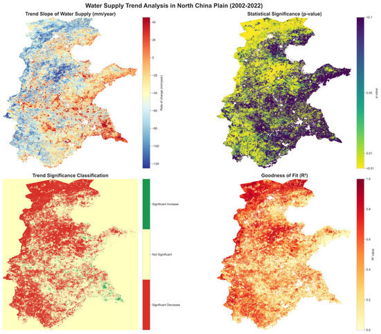
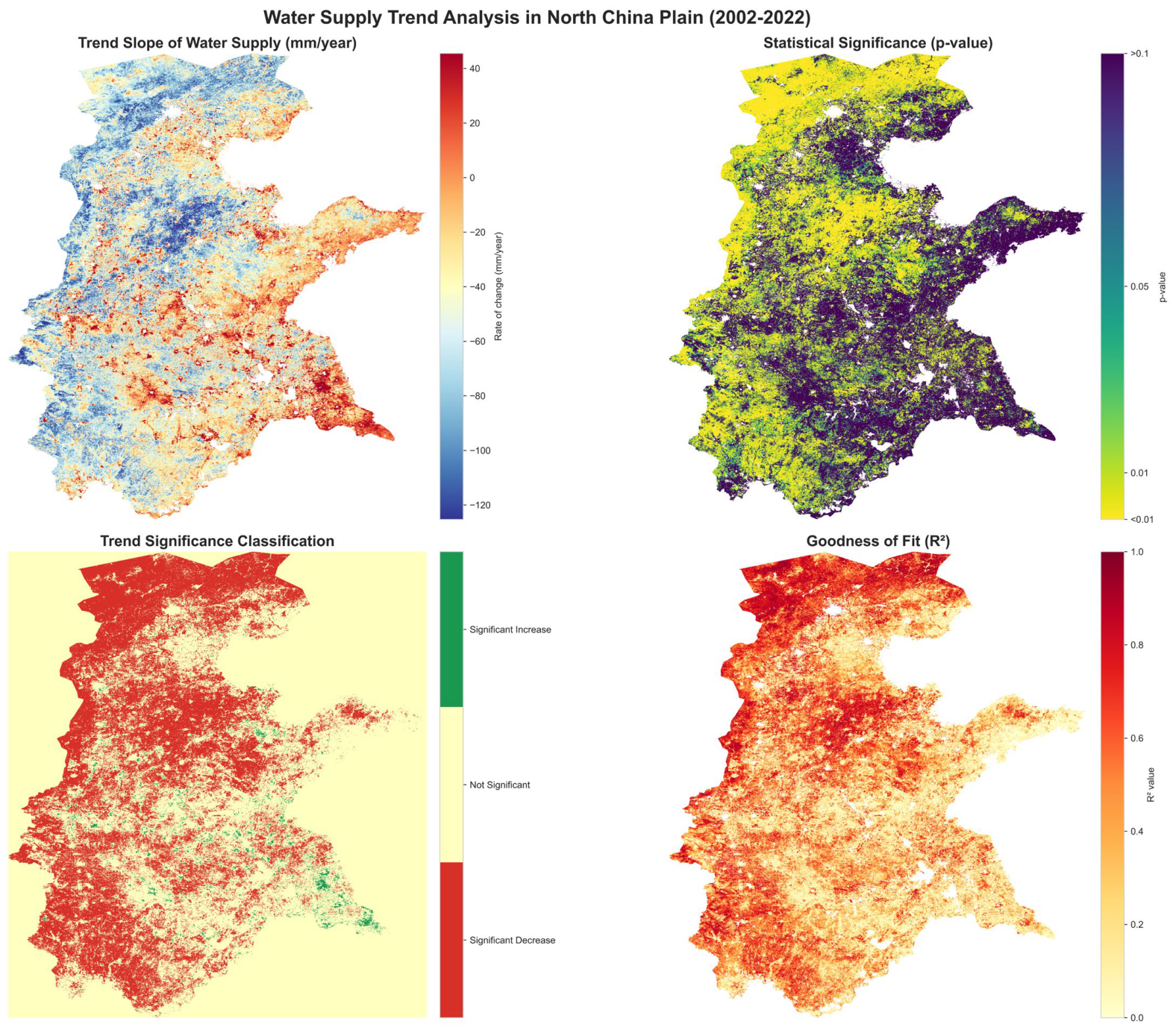
The MK test results provide a more nuanced understanding of these temporal shifts at the pixel level. Approximately 53.4% of the study area exhibits significant temporal trends (p < 0.05), indicating that over half of the North China Plain has undergone non-random, systematic changes in water resource supply over the past two decades. Within these significant areas, the distribution is highly asymmetrical: significant increases are primarily localized in the southeastern and coastal sectors, while significant decreases occupy a more extensive proportion of the central and western regions (Figure 3).
Figure 3.
Spatial Patterns of Water Supply Trends and Statistical Significance in the North China Plain (2002–2022).
This high proportion of pixel-level significance stands in contrast to the regional average, where opposing local trends often mask one another, leading to a non-significant overall mean trend. The prevalence of significant decreases over significant increases further underscores the growing pressure on regional water availability. In addition, the relatively low to moderate goodness-of-fit (R2) values suggest that while over half the region shows a clear directional shift, the remaining 46.6% of the area is dominated by strong interannual fluctuations driven by complex interactions between climatic variability and human interventions.
The pixel-level spatiotemporal characteristics of water supply changes in the North China Plain from 2002 to 2022 were analyzed through four dimensions: water supply trend slope, statistical significance (p-value), trend significance classification, and goodness of fit (R2). At the pixel level, among 3,076,782 valid pixels, 53.4% showed significant changes (p < 0.05), with “significant increase” and “significant decrease” accounting for 2.2% and 51.3%, respectively. At the overall regional level, water supply exhibited a declining trend (average slope−42.9949 mm/year). Although the average p-value (0.1736) did not reach the strong significance threshold of p < 0.05, the average R2 (0.3966) indicates that the model has a certain explanatory power for changes in water supply. Spatially, both the magnitude and significance of water supply trends displayed notable heterogeneity (as visually reflected in the blue-to-red gradient in the trend slope map and the widespread distribution of “significant decrease” in the trend significance classification map).
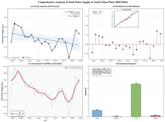
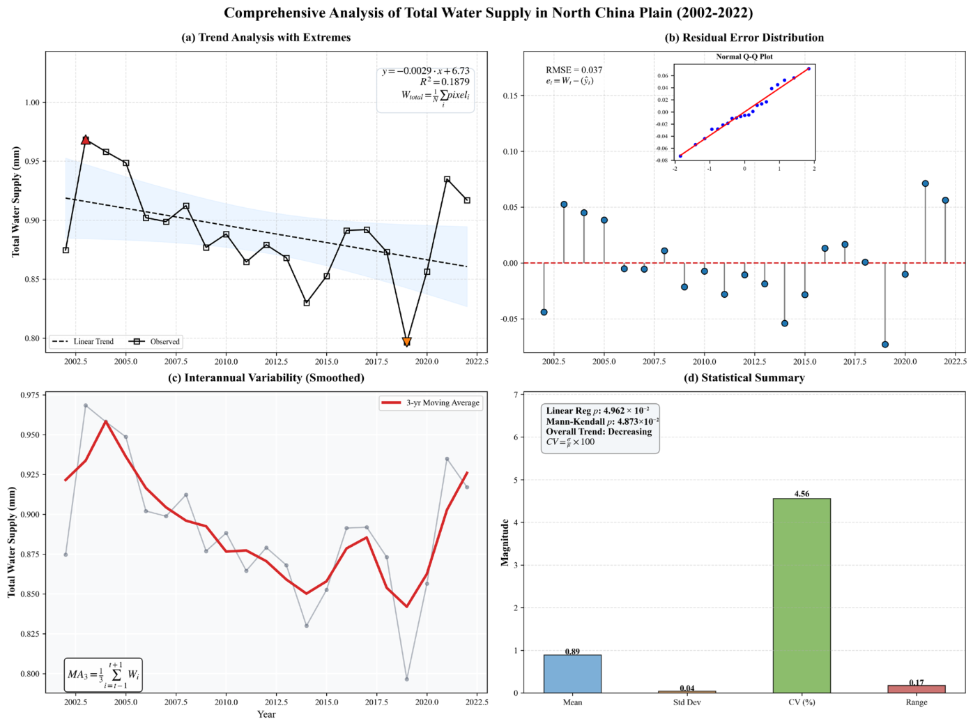
A systematic analysis based on observational data from 2002 to 2022 (Figure 4) indicates a significant declining trend in water resource supply in the North China Plain (linear slope = −1.97722 billion m3/year, p = 0.0475), suggesting a continuous deterioration of water resource availability in this region. Statistical analysis shows that the average annual water resource supply is 602.187 billion m3, with a standard deviation of 28.065 billion m3 and a coefficient of variation of 4.66%, reflecting a moderate degree of interannual fluctuation. Residual analysis (RMSE = 246.330, MAE = 196.899) and the Q-Q plot confirm that the model residuals are approximately normally distributed, enhancing the reliability of the trend analysis. The 3-year moving average curve further reveals the overlapping characteristics of short-term fluctuations and the long-term declining trend in water resource supply, which peaked in 2003 and reached a pronounced low in 2019. This changing trend poses a severe challenge to water security in the North China Plain, necessitating the implementation of adaptive water resource management strategies to address the continuously declining water supply situation.
Figure 4.
Comprehensive Temporal Analysis of Total Water Supply in the North China Plain (2002–2022).
Taken together, the observed long-term decline in water resource supply, combined with the increasing pressures from population growth and rapid economic development, poses a significant challenge to regional water security in the North China Plain and highlights the urgent need for adaptive and sustainable water resource management strategies.
- Trend: The contribution of external water transfer has increased significantly, while changes in natural components are minimal.
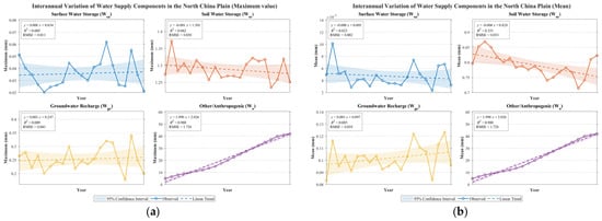
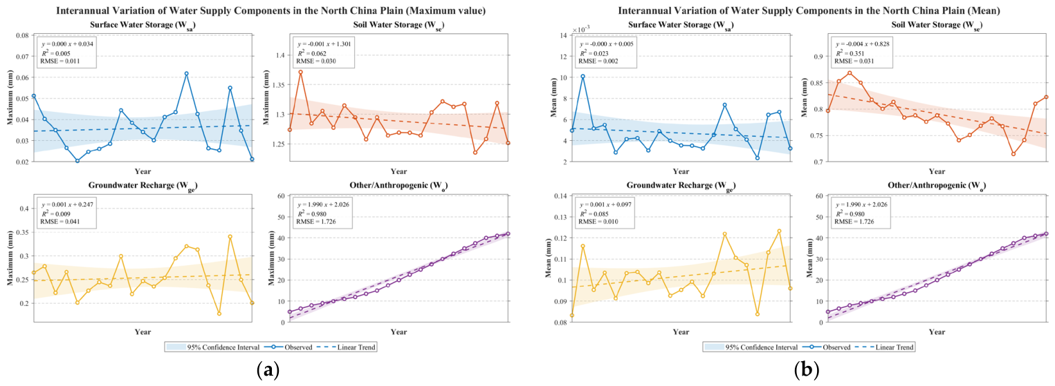
Figure 5a shows that the linear trend slopes of each component differ significantly: Wo exhibits a significant positive trend (slope = 1.990 mm/yr), indicating that in years of extreme drought or under high water demand scenarios, the water supply contribution from inter-basin transfer projects increases sharply; Wse shows a slight decline (slope = −0.001 mm/yr), Wsa shows a slight increase (slope = 0.001 mm/yr), and Wsa has no significant trend (slope = 0.000 mm/yr). Figure 5b (mean dimension) further confirms that the mean slope of Wsa is close to 0 (−0.000 mm/yr) with an RMSE of only 0.002, indicating that the average level of surface water storage has no long-term change. Comparatively, external water transfers are the only water supply component showing a significant increasing trend, highlighting the key role of human-engineered regulation in addressing regional water scarcity; in contrast, the natural components (Wse, Wge) show weak trends, reflecting their slow adjustment under climate change and local water use pressures.
Figure 5.
Interannual Variation of Water Supply Components in the North China Plain. (a) Maximum Values; (b) Mean. (Different colors denote distinct components: blue for surface water storage (Ws), orange for soil water storage (Wv), yellow for groundwater recharge (Wg), and purple for other/anthropogenic contributions (Wo). Solid lines represent observations, dashed lines indicate linear trends, and shaded regions correspond to the 95% confidence intervals).
- 2.
- Volatility: The uncertainty of external water supply is high, while natural hydrological processes are relatively stable.
The reliability of the model is quantified using RMSE and a 95% confidence interval. The RMSE of Wo reaches 1.726, significantly higher than that of the natural components (0.011–0.041), which directly reflects that the external water supply is affected by multiple human and natural factors such as engineering scheduling, inflows from water source areas, and policy objectives, resulting in large interannual variability and high uncertainty. In contrast, the low RMSE values of Wse (RMSE = 0.030), Wge (RMSE = 0.041), and Wsa (RMSE = 0.011–0.002) indicate that natural hydrological processes are mainly dominated by climate sequences (precipitation-evapotranspiration), with relatively stable interannual variability and stronger predictability. The 95% confidence interval shows that the positive trend of Wo is highly likely not to include 0, indicating a significant trend, whereas the slopes of the natural components are close to 0 and their confidence intervals cover 0, not reaching statistical significance.
- 3.
- Contribution Structure: Soil Water as the Absolute Dominant, External Water as a Key Supplement
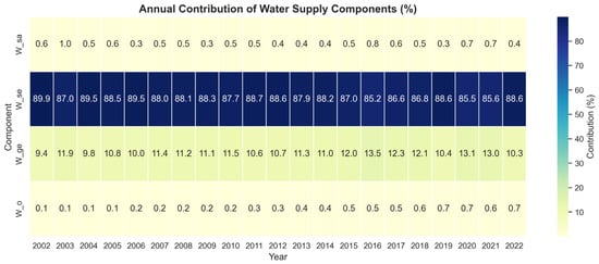
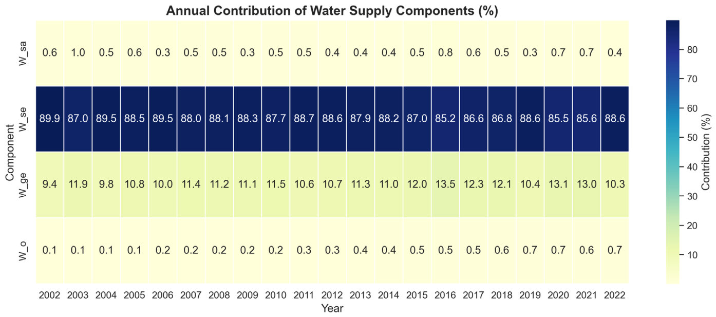
Figure 6 clearly reveals the long-term structure of regional water supply contributions: Wse accounts for as much as 80–90%, making it the absolute core and stable cornerstone of water supply in the North China Plain, thanks to the region’s strong soil water storage capacity in the vadose zone; Wge comes next (10–15%), with its proportion fluctuating in response to interannual variations in precipitation infiltration; Wsa and Wo each account for a very small share (about 1%), making limited direct contributions to total water supply. However, combined with trend analysis, although Wo’s annual average proportion is low, its significant upward trend in peak values clearly indicates its role as a ‘strategic emergency reserve’ during extreme drought years or peak water usage periods. The dominant position of Wse also implies system vulnerability—if its slight declining trend continues, it will directly undermine the foundation of regional water supply security.
Figure 6.
Annual Contribution of Water Supply Components (%).
- 4.
- Driving Mechanisms and Insights
The low trend slopes and low RMSE of the natural components (Wse, Wge, Wsa) indicate that the natural water cycle processes determined by regional climate models remain relatively stable on an interannual scale. However, the slight degradation suggests that soil reservoirs are under long-term depletion pressure. The high growth trend and high volatility of Wo accurately characterize the features of large-scale water transfer projects as external water sources: they are key human solutions to local water resource deficits, but their supply is constrained by distant water source conditions, project capacity, and operational decisions, thereby introducing new uncertainties.
Overall, the water supply system of the North China Plain has developed a dual structure characterized by ‘primarily stable soil water, supplemented by externally transferred water.’ In the future, water resource management should focus on protecting and restoring local natural water storage capacity (particularly Wse), while optimizing the scheduling and efficiency of externally transferred water use, and evaluating its long-term sustainability to mitigate the risks associated with its variability.
4.2. Analysis of the Driving Factors of Water Resource Supply
4.2.1. Selection of the Main Driving Factors for Water Resource Supply
This study focuses on the water resource system of the North China Plain, aiming to systematically identify the key driving factors of water resource dynamic evolution through the integration of machine learning methods, and to conduct an in-depth comparison of the performance differences between XGBoost and Random Forest, two ensemble learning algorithms, in evaluating the importance of hydrological features. The research integrates a multi-source dataset covering four major dimensions: climate, soil, topography, and socio-economics. Specifically, the core indicators include: NDVI, Temp&Prec, PET, Clay, AWC, Sand, Silt, Elev, Slope, GDP, and PopDens.
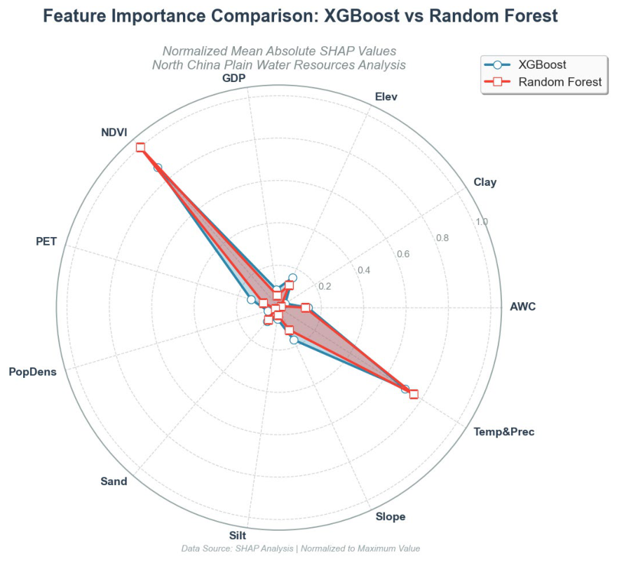
Methodologically, this study employs SHAPvalues to quantify the marginal contribution of each feature to the model’s predictive output. This approach, based on the principles of cooperative game theory, provides a theoretically sound explanatory framework for feature importance assessment. By combining multidimensional visualization with quantitative evaluation, the study constructs a comprehensive model interpretation system: (1) radar plots visualize the priority ranking of feature importance, revealing the similarities and differences between models in identifying driving factors; (2) beeswarm plots depict the nonlinear response relationship between feature values and SHAP values, elucidating feature action mechanisms; (3) a comprehensive evaluation metric system (mean squared error MSE, root mean squared error RMSE, mean absolute error MAE, coefficient of determination R2) quantifies the model’s predictive accuracy, ensuring the reliability of the interpretation results. This multi-scale analysis framework not only achieves precise identification of the key driving factors of the water resource system but also provides methodological support for the interpretable application of machine learning models in the hydrology and water resources field.
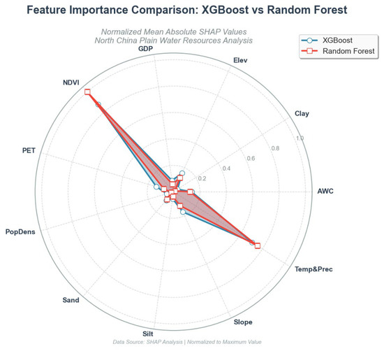
Model interpretability analysis (Figure 7) reveals that the two ensemble learning algorithms, XGBoost and Random Forest, exhibit a high degree of consistency in the ranking of key feature importance. SHAP value analysis indicates that NDVI and Clay dominate the feature importance spectrum, with their mean absolute SHAP values significantly higher than those of other variables. Following them are socioeconomic indicators such as GDP and PopDens, while features like PET, AWC, and Slope have relatively lower importance. This finding carries significant hydro-ecological implications: vegetation coverage regulates surface energy balance and water cycle processes, soil texture characteristics influence water infiltration and retention capacity, and human socioeconomic activities affect the intensity of water resource utilization. Together, these constitute the three core driving dimensions of water resource system evolution in the North China Plain. This result is highly consistent with the theoretical expectations of the vegetation-soil-human activity synergistic regulation mechanism under the ‘nature-society’ dual water cycle framework, providing empirical support for understanding the complex response mechanisms of water resource systems in areas of high-intensity human activity.
Figure 7.
Radar Chart Comparing Feature Importance of XGBoost and Random Forest Models.
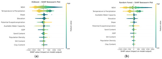
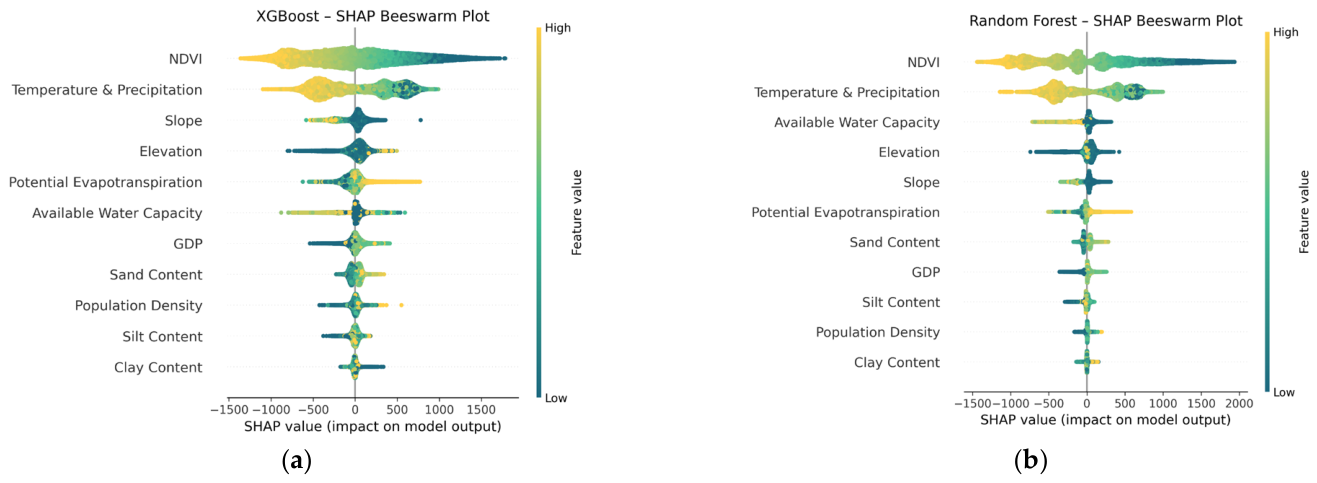
A deep analysis of the SHAP summary plot (As shown in Figure 8a,b) further reveals the directionality and intensity heterogeneity of feature effects. In the XGBoost model, NDVI exhibits a significant threshold effect: when NDVI values are in the high range (corresponding to warm-colored data points in the figure), SHAP values are concentrated in the positive range of 0~1500, indicating that high vegetation coverage has a significant positive driving effect on water resource system output variables (such as surface runoff and groundwater recharge); conversely, low NDVI values (cool-colored data points) mainly cluster in the negative SHAP value region, revealing the inhibitory effect of vegetation degradation on water resource maintenance. Notably, high-value samples of Temp&Prec also significantly shift to the positive SHAP value region (p < 0.05), a phenomenon that mechanistically validates the fundamental role of climatic and hydrological factors in regional water resource replenishment processes. Comparative analysis shows that the Random Forest model exhibits unique nonlinear response characteristics: the distribution range of NDVI SHAP values significantly expands (−1500~2000), and the separation of data points in high and low value ranges is more pronounced (Kolmogorov–Smirnov test, D = 0.68, p < 0.01), reflecting the model’s stronger capability to capture complex nonlinear responses to vegetation cover changes. However, topographic factors (such as Elevation and Slope) in both models show a dispersed distribution of SHAP values (standard deviation > 400), and this spatial heterogeneity suggests that the influence of topographic elements on water resources exhibits significant scale-dependency and regional specificity, potentially arising from the complex surface-groundwater interaction mechanisms in the North China Plain.
Figure 8.
Direction and Distribution of Feature Influence. (a) SHAP Beeswarm Plot of the XGBoost Model; (b) SHAP Beeswarm Plot of the Random Forest Model.
After optimization with the Particle Swarm Optimization (PSO) algorithm, the predictive performance metrics of the XGBoost and Random Forest models indicate that XGBoost outperforms the Random Forest model in mean squared error (MSE = 251,634), root mean squared error (RMSE = 501.63), mean absolute error (MAE = 367.23), and coefficient of determination (R2 = 0.8013), whereas the corresponding metrics for Random Forest are MSE = 323,775, RMSE = 569.01, MAE = 424.23, and R2 = 0.7443. Both models markedly surpass the baseline performance of predicting only the mean without a model (R2 = 0.0000), confirming the effectiveness of the optimized gradient boosting tree models for this task. The evaluation metrics of the optimized models (Table 4) show that XGBoost significantly outperforms Random Forest across all error and goodness-of-fit indicators.
Table 4.
Performance Evaluation of XGBoost and Random Forest.
4.2.2. Analysis of Interannual Variations of Major Driving Factors
Obtain the following information from the above image (Figure 9):
Figure 9.
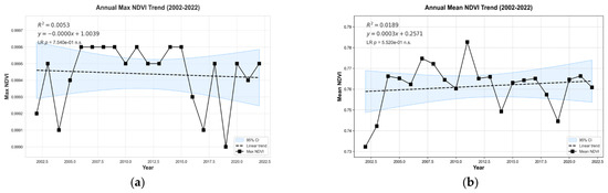
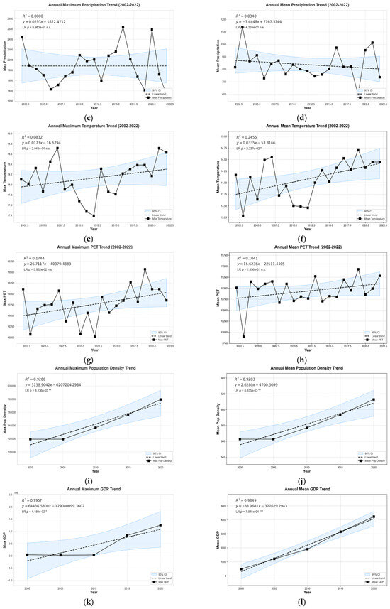
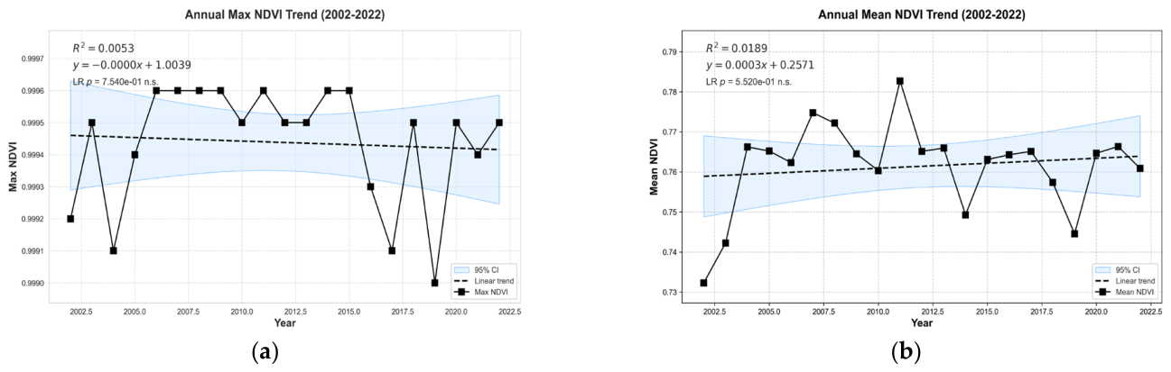
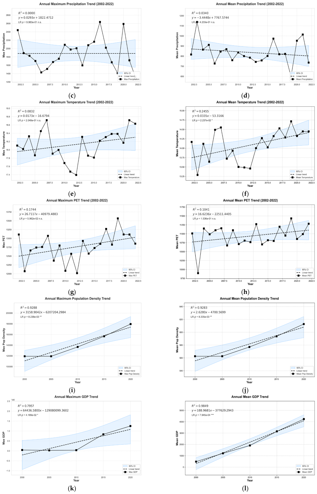
Annual trends of NDVI, climatic, and socioeconomic factors. (a) Annual Max NDVI Trend (2002–2022); (b) Annual Mean NDVI Trend (2002–2022); (c) Annual Maximum Precipitation Trend (2002–2022); (d) Annual Mean Precipitation Trend (2002–2022); (e) Annual Maximum Temperature Trend (2002–2022); (f) Annual Mean Temperature Trend (2002–2022); (g) Annual Maximum PET Trend (2002–2022); (h) Annual Mean PET Trend (2002–2022); (i) Annual Maximum Population Density Trend; (j) Annual Mean Population Density Trend; (k) Annual Maximum GDP Trend; (l) Annual Mean GDP Trend. Note: *, **, and *** indicate statistical significance at the p < 0.05, p < 0.01, and p < 0.001 levels, respectively. ‘n.s.’ stands for not significant (p ≥ 0.05).
PET, as a key indicator of regional energy balance and water consumption, exhibited relatively weak fluctuations in both its maximum and mean values (Figure 9g,h). Between 2002 and 2022, the maximum PET ranged from 12,000 to 13,600 mm, with a linear regression goodness-of-fit of R2 = 0.174 and a slope of 26.03 mm/year. Although the MK test indicated a significant upward trend (p = 4.197 × 10⁻² *), the linear regression p-value (5.962 × 10⁻²) did not reach significance, suggesting considerable interannual variability in PET peaks. The mean PET remained within 9500–11,500 mm (R2 = 0.104), with neither linear regression nor MK tests reaching significance (p > 0.05), indicating that overall regional evapotranspiration and water consumption were relatively stable. As a core hydrological driver, precipitation maxima showed no significant trend, fluctuating between 16 and 20 mm from 2002 to 2022 (R2 = 0.08), with a near-zero linear regression slope and non-significant statistical tests (p > 0.05) (Figure 9c). In contrast, mean precipitation exhibited a significant increasing trend, rising from 12 mm in 2002 to 16 mm in 2022 (R2 = 0.25), with both linear regression (p = 2.237 × 10⁻²) and MK test (p = 1.868 × 10⁻²) achieving significance (Figure 9d). The Sen’s slope of 0.04 mm/year indicates a gradual increase in regional water input, which may provide favorable conditions for enhanced ecosystem productivity.
The NDVI maximum (Figure 9a) has consistently remained in a high range of 0.9990–0.9996, indicating that regional vegetation coverage has nearly reached saturation. The linear regression R2 is only 0.005, with a slope approaching 0, and statistical tests are not significant (p > 0.05), indicating that vegetation coverage has been stable over the long term, without significant impact from human activities or climate fluctuations, and that the vegetation component of the ecosystem exhibits strong resistance to disturbances.
The proportion of irrigated farmland, as a direct indicator of agricultural production activities, exhibited a highly significant decreasing trend between 2002 and 2022, declining from 0.06 to 0.05 (R2 = 0.94). Both the linear regression (p = 5.472 × 10⁻¹³) and the MK reached highly significant levels, with a Sen’s slope of −0.0004 per year. This trend suggests that the regional agricultural planting structure may be shifting toward dryland farming or non-agricultural land, or that improvements in irrigation efficiency have led to a reduced proportion of irrigated area. In contrast, the maximum NDVI has consistently remained within a high range of 0.9990–0.9996 (Figure 9a), indicating that regional vegetation coverage has nearly reached saturation. The linear regression goodness-of-fit is low (R2 = 0.005), the slope is near zero, and both linear regression and MK tests are not significant (p > 0.05), suggesting that vegetation coverage has remained stable over the long term. These results imply that the vegetation component of the ecosystem exhibits strong resistance to disturbances, with minimal impact from human activities or interannual climate fluctuations.
Population density and GDP, as direct indicators of human activity, both exhibited highly significant upward trends between 2000 and 2020. The maximum population density increased from approximately 100,000 people/km2 to over 200,000 people/km2 (R2 = 0.93), with both linear regression (p = 8.236 × 10⁻³ *) and the MK test (p = 2.298 × 10⁻²) reaching significance. The Sen’s slope of 3611.69 people/(km2·year) reflects a strong regional population agglomeration effect. The mean population density also steadily increased from 500 people/km2 to 675 people/km2 (R2 = 0.93), with similarly significant statistical tests (p < 0.01), indicating continuously increasing population pressure as shown in Figure 9i,j. Economic development, represented by GDP, grew even more rapidly. The maximum GDP increased from nearly 0 million yuan/km2 in 2000 to 250,000 million yuan/km2 in 2020 (R2 = 0.83), with a linear regression slope of 8667.0 million yuan/(km2·year), indicating a highly significant upward trend. The mean GDP also rose from 1000 million yuan/km2 to 2600 million yuan/km2 (R2 = 0.99), with a slope of 172.1 million yuan/(km2·year), reflecting an almost perfect linear growth and highlighting the profound impact of rapid regional economic development on land use and ecological processes as shown in Figure 9k,l.
The driving factors in the study area exhibit a ‘two increases, two stabilities, and one decrease’ evolutionary pattern: population density and GDP show a highly significant increase, mean precipitation shows a significant increase, PET and NDVI remain stable, and the proportion of irrigated farmland decreases significantly. This combination may have complex impacts on ESVw: economic growth and population aggregation may increase ecological pressure, but increased precipitation and reduced irrigated farmland may alleviate some of this pressure, while stable vegetation coverage provides a fundamental guarantee for ESVw. Subsequent studies need to quantify the relative contributions of each factor through a coupled model to provide scientific support for watershed ecological protection and sustainable development.
4.2.3. Analysis of the Correlation Between Major Driving Factors and Water Resource Supply
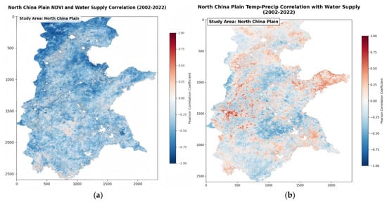
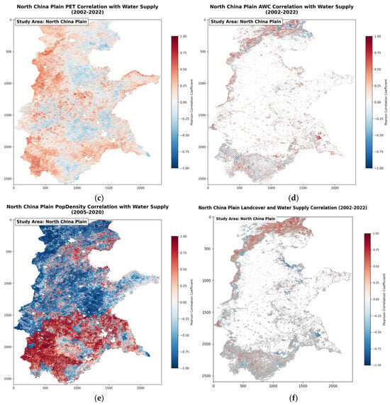
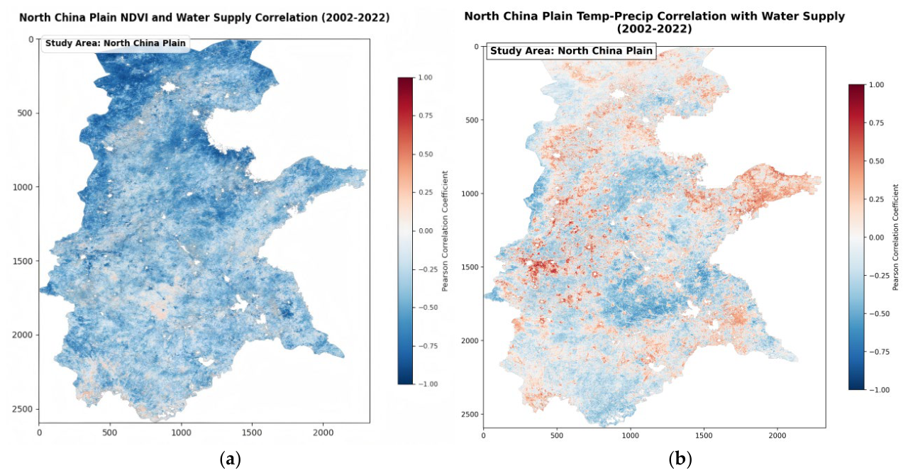
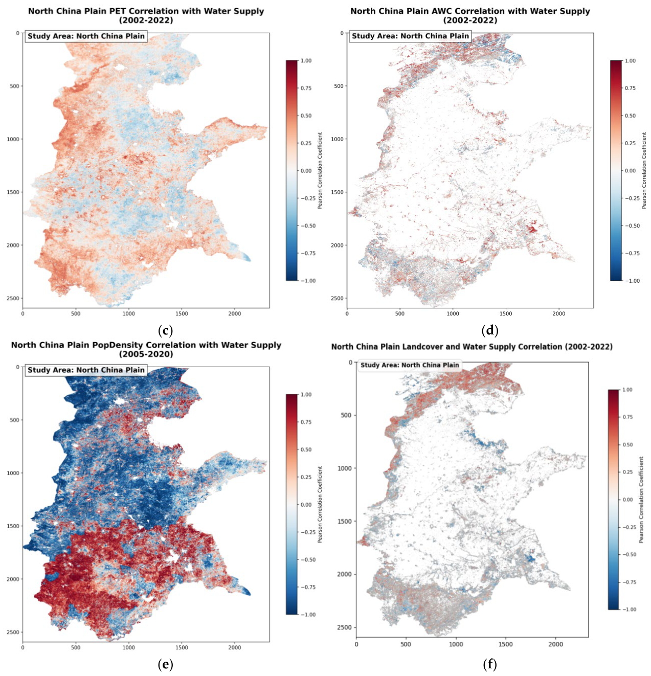
A comprehensive spatial correlation analysis of multi-source data from the North China Plain for 2002–2022 (Note: population density data are from 2005–2020) As shown in Figure 10 indicates that the core driving mechanism of water resource supply in this region is characterized by ‘being dominated by socio-economic pressures, exhibiting regional differentiation in natural hydrological conditions, and involving complex interactions between humans and the environment’.
Figure 10.
Analysis of the Correlation Between Major Driving Factors and Water Resource Supply. (a) Correlation with NDVI (2002–2022); (b) Correlation with Temperature-Precipitation (2002–2022); (c) Correlation with Potential Evapotranspiration (PET) (2002–2022); (d) Correlation with Available Water Capacity (AWC) (2002–2022); (e) Correlation with Population Density (2005–2020); (f) Correlation with Landcover (2002–2022).
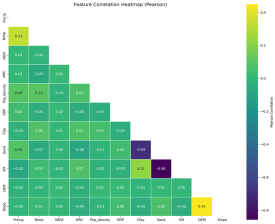
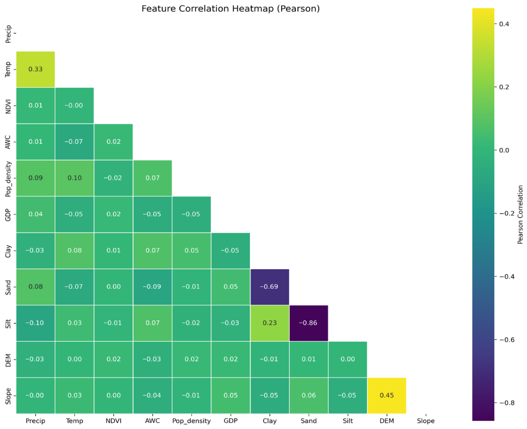
This Pearson correlation coefficient heatmap (Figure 11) visually represents the strength and direction of linear correlations between various features through a color gradient (yellow to purple), where yellow areas indicate strong positive correlations and purple areas indicate strong negative correlations.
Figure 11.
Feature Correlation Heatmap (Pearson).
- Natural Ecological Factors: Bidirectional Regulation and Spatial Trade-offs between Vegetation and Soil
Natural ecological factors regulate water resources through the dual pathways of ‘vegetation water consumption-conservation’ and ‘soil water storage-leakage.’ The correlation between NDVI and water resource supply (Figure 10a) shows a pattern of ‘overall negative correlation, local positive correlation’: most areas of the North China Plain (especially agricultural intensive and semi-arid transitional zones) appear light blue to blue (correlation coefficient −0.25 to −1.00), indicating that high vegetation cover (high NDVI values) is accompanied by intense evapotranspiration, exacerbating water resource depletion; only in ecological conservation areas (such as the forested slopes of the Taihang Mountains) do light red patches appear (correlation coefficient 0.1 to 0.5), confirming the nonlinear threshold effect whereby high vegetation coverage enhances water supply through root water retention and canopy interception. The correlation of AWC (Figure 10c) further reveals the regulatory role of soil texture: areas with higher clay content (such as around the old course of the Yellow River) appear red (correlation coefficient 0.3 to 1.00), indicating that high AWC enhances soil water reservoir regulation capacity and mitigates precipitation fluctuations; sandy soil areas (such as the coastal plains) appear blue (correlation coefficient −0.5 to −1.00) due to intensified leakage leading to the loss of available water resources. The correlation of land cover (Figure 10f) highlights the impact of human activities on the underlying surface: forested and wetland-covered areas in the southern slopes of the Yanshan Mountains in the north and the Huang-Huai Plain in the south appear red (correlation coefficient 0.5 to 1.00), playing a positive conservation role by intercepting precipitation and increasing infiltration; central plain inland areas (central and southern Hebei) in which construction land and farmland are expanding appear blue (correlation coefficient −0.5 to −1.00), as hardened surfaces and water-intensive crop cultivation reconstruct the water cycle, resulting in runoff loss and encroachment on ecological water use.
- 2.
- Hydrological and Climatic Factors: Background Drivers of Climate Fluctuations and Evapotranspiration Stress
Hydro-climatic factors constitute the primary exogenous drivers governing water resource supply, with their spatiotemporal coupling representing a dynamic equilibrium between “precipitation recharge” and “evapotranspiration depletion.” The spatial heterogeneity of the correlation between the Temperature–Precipitation (Temp-Precip) nexus and water supply (Figure 10b) delineates distinct hydro-climatic regimes: positive correlations (red zones, r = 0.4 to 1.00) dominate the southeastern monsoon-influenced regions (e.g., the Shandong Peninsula), indicating that abundant precipitation effectively offsets thermal losses, thereby sustaining water replenishment. Conversely, negative feedback loops (blue zones, r = −0.3 to −1.00) are observed in the northwest (e.g., west of the Taihang Mountains), where warming exacerbates evapotranspiration (ET) losses, manifesting as a “precipitation-evapotranspiration deficit.” Furthermore, the correlation analysis of Potential Evapotranspiration (PET) (Figure 10d) quantifies the spatial intensity of atmospheric water demand. In the Central Plains (e.g., Shijiazhuang), strong negative correlations (dark blue, r = −0.8 to −1.00) signify that high-temperature and low-humidity regimes induce a surge in PET, acting as a primary constraint on water availability. In contrast, marginal high-altitude areas (e.g., the Yanshan Mountains) show weak positive correlations (light red, r = 0.2 to 0.6), reflecting lower water consumption pressures and a relatively stable supply–demand balance.
- 3.
- Human Activity Factors: The Bidirectional Stress of Population Density and Land Cover
Human activity factors fundamentally reshape regional water resource patterns through demand-side pressures and supply-side modifications. The correlation between PopDens and water supply (Figure 10e) manifests a distinct “red-blue mosaic” spatial pattern: Southeastern irrigated agricultural zones (e.g., eastern Henan) exhibit positive correlations (correlation coefficient: 0.25–1.00, red zones), reflecting the capacity of water resources to underpin population agglomeration and industrial-agricultural layouts. In contrast, the Beijing-Tianjin-Hebei urban agglomeration and groundwater overdraft regions display negative correlations (coefficient: −0.25 to −1.00, blue zones), indicating that intensive multi-sectoral water consumption (domestic, industrial, and agricultural) drives resource depletion. Notably, transitional areas characterized by light red or light blue patches suggest that human-water conflicts are mediated by local industrial structures (e.g., water-saving agriculture versus non-agricultural industrialization). Concurrently, Landcover dynamics reinforce these findings (Figure 10d): Negative correlations (−0.5 to −1.00) dominate in rapidly urbanizing central plains, where construction land expansion and high-intensity farming degrade hydrological regulation capacity. Conversely, positive correlations (0.5–1.00) prevail in forested and wetland ecosystems of northern and southern margins, underscoring their role in sustaining water retention and recharge. This dichotomy confirms that anthropogenic land-system modifications directly restructure natural eco-hydrological cycles.
5. Discussion
5.1. The Impact of Topography and Climate Factors on Water Resource Supply
From the perspective of topography, the SHAP value distributions for elevation and slope are scattered and exhibit relatively low average contributions, reflecting that the North China Plain’s predominantly flat terrain (plains covering over 95% of the area) limits the redistributive influence of topography on runoff accumulation and groundwater recharge. However, the high variability of SHAP values for topographic factors (standard deviation > 400) in the SHAP swarm plot indicates that, at the local scale, microtopographic variations can still exert nonlinear regulatory effects on water resource supply by influencing surface flow paths and soil water retention times. Climatic factors show more pronounced directional and threshold characteristics. High-value samples of the combined temperature–precipitation index are skewed toward positive SHAP values, confirming that precipitation input is a primary controlling variable for regional water supply. Notably, the spatial correlation between potential evapotranspiration (PET) and water supply exhibits a distinct northeast–southwest differentiation: in the water-rich southwest, high PET coexists with high water supply, indicating that net water resources (precipitation minus evapotranspiration) remain sufficient; in contrast, in the precipitation-deficient northeast, high PET exacerbates drought stress and negatively correlates with water supply. This spatial heterogeneity underscores the critical role of hydrological and thermal balance in shaping regional water resource endowment. Furthermore, the overall negative correlation between NDVI and water supply confirms the complex coupling between climate and vegetation processes: in this high-intensity agricultural region, maintaining vegetation cover often depends on irrigation rather than natural precipitation, forming a unique human–water–ecology relationship characterized by “green growth through irrigation” rather than “water abundance nurturing greenery.”
5.2. The Impact of Human Activity Factors on Water Resource Supply
From an economic perspective, GDP and water resource supply are strongly negatively correlated across most regions (Pearson coefficient near −1), indicating that the water demand driven by industrialization and urbanization often exceeds local water resource capacity. High-GDP areas coincide with hydrogeological units experiencing substantial groundwater over-extraction and surface water utilization rates exceeding 80%, illustrating the trade-off between economic development and water security. Population density exhibits a clear north–south differentiation pattern. In southern regions (Henan and central–southern Shandong), population density is positively correlated with water supply, reflecting targeted water allocation to densely populated areas via inter-basin transfer projects such as the Middle Route of the South-to-North Water Diversion Project. Conversely, in northern regions (Hebei and Shanxi), population density negatively correlates with water supply, demonstrating that in areas without effective external water transfers and with limited local water endowment, population aggregation intensifies supply–demand tensions. These findings provide empirical evidence for the spatial restructuring effects of water transfer projects on regional human–water interactions. Regarding agricultural activities, the continuous decline in irrigated farmland (Sen’s slope −0.0004/year, p < 0.01), combined with the dominant role of soil water (accounting for 80–90% of total supply), suggests that while crop structure adjustments and water-saving technologies may alleviate some pressures, deep soil water reservoirs remain under long-term extraction, representing a potential vulnerability to regional water security. The rapid growth and high volatility of externally transferred water further illustrate the dual nature of human-engineering interventions: while they provide strategic reserves to compensate local deficits, their reliability is constrained by source-area inflows and scheduling decisions, introducing additional uncertainty into regional water security.
5.3. Policy and Management Recommendations
Based on the above analyses, this study proposes targeted management strategies along three dimensions: water resource allocation optimization, ecological resilience enhancement, and institutional collaborative governance.
1. Regionally differentiated water resource management. Spatial correlations indicate significant north–south disparities in the effects of GDP and population density on water supply, suggesting that management zones should be delineated according to driving factor intensity. In northern regions with strong negative correlations (Hebei, Shanxi), strict dual control over groundwater extraction and water levels is recommended, along with accelerated adoption of water-saving technologies and optimized crop structures to reduce high-water-consuming crops. In southern regions with positive correlations, scheduling flexibility for inter-basin transfer projects and strengthened ecological compensation mechanisms are crucial to mitigate risks associated with long-distance water transfers.
2. Synergistic soil water conservation and vegetation restoration. Given that soil water constitutes 80–90% of total supply and exhibits slight degradation, it should be integrated into a unified management framework. Agronomic practices such as conservation tillage, straw return, and enhanced organic fertilization are recommended to improve soil water retention. Considering the negative NDVI–water supply correlation, restoration projects should prioritize drought-tolerant native species and avoid indiscriminate greening that exacerbates water consumption.
3. Climate-adaptive water allocation. Rising PET and hydrothermal zonation differences highlight potential drought exacerbation under warming scenarios. Incorporating meteorological forecasts into annual allocation planning, dynamically adjusting surface–groundwater ratios, and maintaining ecological water red lines are recommended to preserve river, lake, and wetland functions.
4. Collaborative governance of the natural–economic water cycle. The increasing contribution of external water transfers emphasizes human engineering in the regional water cycle. Given their volatility, cross-basin risk warning and reserve systems should be established. Additionally, integrating ecosystem service value (ESV) assessments into planning and compensation mechanisms, alongside market-based water rights trading, can align economic development with water resource protection.
5.4. Limitations and Future Research Directions
The modeling framework proposed in this study, which integrates Particle Swarm Optimization (PSO) with XGBoost and Random Forest, provides a robust approach for high-precision prediction and mechanism analysis of regional water resource supply. This combination enables automated hyperparameter optimization, strong nonlinear fitting, and systematic evaluation of the contributions of environmental and socioeconomic drivers via SHAP values, representing a methodological advancement in the quantitative assessment of water ecosystem services. While the classification methods employed in this study are well established, they do not incorporate some of the latest advances in time-series modeling. Recent studies have demonstrated that temporal–contextual self-supervised learning leverages the inherent temporal and contextual structure of time-series data to achieve efficient automated fault detection without requiring extensive labeled samples, enhancing sensitivity to both short-term fluctuations and long-term trends [22]. Similarly, class-aware temporal and contextual contrastive frameworks integrate class information with contrastive learning to improve semi-supervised fault detection, enabling the model to distinguish rare or minority events and utilize unlabeled data to strengthen feature representations [23]. Future research could explore integrating these approaches into water resource supply modeling to enhance robustness and capture richer temporal–contextual patterns.
6. Conclusions
Between 2002 and 2022, the water resource supply in the North China Plain showed a significant declining trend, decreasing by approximately 1.98 billion cubic meters per year on average (p < 0.05). The regional water supply structure is dominated by soil moisture, accounting for 80% to 90% of the total, while water transferred from other regions, though limited in total proportion, exhibited a prominent growth rate and notable interannual fluctuations.
Analysis of driving mechanisms indicates that vegetation cover (NDVI), clay content, gross domestic product (GDP), and population density are the primary factors controlling the dynamics of water supply. Notably, GDP shows a strong negative correlation with water resource supply across most areas. This negative relationship underscores the “trade-off” between socio-economic expansion and ecological maintenance; higher GDP levels typically signify intensive industrial clusters and advanced urbanization, which inevitably increase water withdrawal for production and domestic consumption, thereby exerting substantial pressure on the natural water cycle and diminishing ecosystem-based supply capacity. In contrast, population density exhibits a significant north–south differentiation closely associated with inter-basin water transfer projects, indicating that human-induced water reallocation partially mitigates localized water stress. At the climatic level, combined temperature–precipitation indices and potential evapotranspiration play fundamental regulatory roles, while topographic factors have limited influence due to the flat terrain of the North China Plain.
In terms of methodology, this study established a novel comparative analysis framework using dual models of PSO-XGBoost-SHAP and PSO-RF-SHAP. Model evaluation results indicate that the PSO-XGBoost model’s predictive accuracy (R2 = 0.8013) significantly outperforms that of the PSO-RF model (R2 = 0.7443), demonstrating stronger fitting capability in capturing multivariate nonlinear response relationships. This methodological integration not only enhances prediction accuracy but also provides interpretable insights into complex hydrological–human interactions through SHAP values, representing a distinctive contribution beyond previous studies.
Methodological reflections suggest that although ensemble machine learning frameworks excel in identifying drivers, the existing models still have room for improvement in their sensitivity to sudden shifts in water supply during extreme drought years. Additionally, due to data constraints, factors such as actual groundwater extraction intensity and irrigation efficiency were not fully incorporated, which may affect the completeness of attribution results. Future research can be advanced by: (1) incorporating higher-resolution remote sensing ET products and GRACE-based groundwater data; (2) coupling future climate scenarios (SSP-RCP pathways) with land-use simulations; and (3) exploring deep learning models like LSTM or Transformer to enhance early warning capabilities for extreme events.
The academic contributions of this study are highlighted in four key aspects:
1. The PSO–XGBoost–SHAP framework was applied for the first time to analyze water supply driving mechanisms in the North China Plain, achieving a synergistic optimization of accuracy and interpretability.
2. The study quantified the absolute dominant role of soil water (80–90%) and its slight degradation trend, providing critical evidence for shifting the focus of water management from traditional surface-groundwater (“Blue Water”) to soil water reservoirs (“Green Water”) to enhance regional resilience.
3. The dual effects of inter-basin water transfer projects—both as “strategic emergency supplementation” and as a source of “introduced fluctuation risks”—were systematically characterized.
4. From the perspective of spatial heterogeneity, the study clarified the north–south differentiation in the “human–water relationship,” laying a foundation for differentiated policy-making.
In summary, the dynamics of water supply in the North China Plain are the result of the co-evolution of natural hydrological constraints and continuously intensified human activities. Only by integrating a systemic perspective of the “nature–society” dual water cycle, actively coordinating soil water conservation, and implementing fine-tuned demand-side management, can the declining trend of water supply be effectively mitigated. This study provides actionable insights for adaptive water resource management and offers a replicable methodological approach for other water-scarce regions worldwide.
Author Contributions
Conceptualization, X.Z. and M.Y.; methodology, X.Z.; software, X.Z. and Z.L.; validation, Z.L.; formal analysis, X.Z.; investigation, X.Z. and R.C.; resources, M.Y. and Z.X.; data curation, S.W.; writing—original draft preparation, X.Z. and S.W.; writing—review and editing, X.Z., M.Y., and R.C.; visualization, X.Z.; supervision, M.Y. and Z.X.; funding acquisition, M.Y. All authors have read and agreed to the published version of the manuscript.
Funding
This research was funded by the National Natural Science Foundation of China (NSFC), grant number 42474057, and the Guangxi Key Laboratory of Spatial Information and Surveying, grant number 19-050-11–27.
Institutional Review Board Statement
Not applicable.
Informed Consent Statement
Not applicable.
Data Availability Statement
All datasets used in this study are publicly accessible from the aforementioned ERA5-Land, NASA EarthData, MODIS, GPW v4.11, and RESDC sources. The code used for data processing and analysis is available from the corresponding author upon reasonable request.
Conflicts of Interest
The authors declare no conflicts of interest.
Abbreviations
The following abbreviations are used in this manuscript:
| ESV | ecosystem service value |
| Avg. Temp | annual average temperature |
| Avg. Precip | annual average precipitation |
| ET0 | potential evapotranspiration |
| NDVI | normalized difference vegetation index |
| FC-WP | field capacity to wilting point ratio |
| DEM | digital elevation model |
| W | the water resource supply (total amount) |
| Wsa | available surface water |
| Wge | exploitable groundwater |
| Wse | effective soil water |
| Wo | externally transferred water/recycled water/others |
| CV | coefficient of variation |
| MK | Mann–Kendall |
| XGBoost | Extreme Gradient Boosting |
| GBDT | Gradient Boosting Decision Trees |
| SHAP | SHapley Additive exPlanations |
References
- Li, T.; Li, W.; Qian, Z. Variations in ecosystem service value in response to land use changes in Shenzhen. Ecol. Econ. 2010, 69, 1427–1435. [Google Scholar] [CrossRef] [Scilit]
- Cook, B.R.; Spray, C.J. Ecosystem services and integrated water resource management: Different paths to the same end? J. Environ. Manag. 2012, 109, 93–100. [Google Scholar] [CrossRef] [Scilit]
- Priyan, K. Issues and challenges of groundwater and surface water management in semi-arid regions. In Groundwater Resources Development and Planning in the Semi-Arid Region; Springer: Cham, Switzerland, 2021; pp. 1–17. [Google Scholar]
- Liu, C.; Yu, J.; Kendy, E. Groundwater exploitation and its impact on the environment in the North China Plain. Water Int. 2001, 26, 265–272. [Google Scholar] [CrossRef] [Scilit]
- Zhang, Q.; Sun, J.; Zhang, G.; Liu, X.; Wu, Y.; Sun, J.; Hu, B. Spatiotemporal dynamics of water supply–demand patterns under large-scale paddy expansion: Implications for regional sustainable water resource management. Agric. Water Manag. 2023, 285, 108388. [Google Scholar] [CrossRef] [Scilit]
- Yang, L.; Liu, Y.; Liu, Y.; Liu, R. Spatial-temporal dynamics and drivers of ecosystem service interactions along the Yellow River area in Shaanxi Province. J. Clean. Prod. 2025, 496, 145095. [Google Scholar] [CrossRef] [Scilit]
- Li, D.; He, L.; He, Z.; Bai, W.; Jin, R.; Lin, Z.; Huang, Y. Integrating multi-dimensional features for remote sensing–based drought monitoring and driver analysis during the vegetation growing season: A case study in northern Xinjiang. Geomat. Nat. Hazards Risk 2026, 17, 2634962. [Google Scholar] [CrossRef] [Scilit]
- Pagliacci, F.; Pavone, P.; Russo, M.; Giorgi, A. Regional structural heterogeneity: Evidence and policy implications for RIS3 in macro-regional strategies. Reg. Stud. 2020, 54, 765–775. [Google Scholar] [CrossRef] [Scilit]
- Wang, X.; Zhang, S.; Tang, X.; Gao, C. Spatiotemporal heterogeneity and driving mechanisms of water resources carrying capacity for sustainable development of Guangdong Province in China. J. Clean. Prod. 2023, 412, 137398. [Google Scholar] [CrossRef] [Scilit]
- Wu, C.; Xu, Q.; Zhang, X.; Ma, Y. Palaeochannels on the North China Plain: Types and distributions. Geomorphology 1996, 18, 5–14. [Google Scholar] [CrossRef] [Scilit]
- Willis, R.; Finney, B.A.; Zhang, D. Water resources management in north China plain. J. Water Resour. Plan. Manag. 1989, 115, 598–615. [Google Scholar] [CrossRef] [Scilit]
- Wang, E.; Yu, Q.; Wu, D.; Xia, J. Climate, agricultural production and hydrological balance in the North China Plain. Int. J. Climatol. J. R. Meteorol. Soc. 2008, 28, 1959–1970. [Google Scholar] [CrossRef] [Scilit]
- Tan, Y.; Xin, Y.; Guo, C.; Lyu, S.; Zhang, G.; Long, Y.; Zhai, Y.; Packham, H.; Zhou, Y.; Tan, H. Impact of urbanization on baseflow characteristics in the central catchment of North China Plain, China. J. Hydrol. Reg. Stud. 2023, 50, 101527. [Google Scholar] [CrossRef] [Scilit]
- Abdi, H. Coefficient of variation. Encycl. Res. Des. 2010, 1, 169–171. [Google Scholar]
- Ali, R.O.; Abubaker, S.R. Trend analysis using Mann-Kendall, Sen’s slope estimator test and innovative trend analysis method in Yangtze River basin, China. Int. J. Eng. Technol. 2019, 8, 110–119. [Google Scholar]
- Kennedy, J.; Eberhart, R. Particle swarm optimization. In Proceedings of the ICNN’95-International Conference on Neural Networks, Perth, Australia, 27 November–1 December 1995; pp. 1942–1948. [Google Scholar]
- Rini, D.P.; Shamsuddin, S.M.; Yuhaniz, S.S. Particle swarm optimization: Technique, system and challenges. Int. J. Comput. Appl. 2011, 14, 19–26. [Google Scholar] [CrossRef] [Scilit]
- Breiman, L. Random forests. Mach. Learn. 2001, 45, 5–32. [Google Scholar] [CrossRef] [Scilit]
- Biau, G.; Scornet, E. A random forest guided tour. Test 2016, 25, 197–227. [Google Scholar] [CrossRef] [Scilit]
- Li, Z. Extracting spatial effects from machine learning model using local interpretation method: An example of SHAP and XGBoost. Comput. Environ. Urban Syst. 2022, 96, 101845. [Google Scholar] [CrossRef] [Scilit]
- Zhang, H.; Zhu, C.; Jiao, T.; Luo, K.; Ma, X.; Wang, M. Analysis of the Trends and Driving Factors of Cultivated Land Utilization Efficiency in Henan Province from 2000 to 2020. Land 2024, 13, 2109. [Google Scholar] [CrossRef] [Scilit]
- Wang, S. Temporal–Contextual Self-Supervised Time-Series Learning for Automated Fault Detection and Diagnosis of Air Handling Units in Buildings. Build. Environ. 2026, 292, 114300. [Google Scholar] [CrossRef] [Scilit]
- Wang, S. Class-aware temporal and contextual contrastive framework for semi-supervised automated fault detection and diagnosis in air handling units. Energy Build. 2026, 358, 117233. [Google Scholar] [CrossRef] [Scilit]

Disclaimer/Publisher’s Note: The statements, opinions and data contained in all publications are solely those of the individual author(s) and contributor(s) and not of MDPI and/or the editor(s). MDPI and/or the editor(s) disclaim responsibility for any injury to people or property resulting from any ideas, methods, instructions or products referred to in the content. |
© 2026 by the authors. Licensee MDPI, Basel, Switzerland. This article is an open access article distributed under the terms and conditions of the Creative Commons Attribution (CC BY) license.