


Abstract
The increasing number of UAVs performing commercial and amateur flights necessitates the introduction of safe design principles for airborne platform architectures and UAV control algorithms. This article presents an approach to designing such solutions. UAVConfigurator is software designed for simulating the dynamics of a Commercial Off-The-Shelf (COTS) Fighter UAV airframe, developed in the MATLAB/Simulink environment. This application simplifies the design and testing of control software for unmanned systems, and is intended for use by UAV designers, researchers, and students. It serves as a Software-In-the-Loop (SIL) simulator, allowing users to build and test new algorithms in simulated environments before transitioning to real UAVs. The software accurately models UAV dynamics, as confirmed by flight tests, owing to its integration with advanced aerodynamic computations. It includes models of essential UAV components and enables users to simulate sensor failures. Additionally, it features an ISA atmosphere model. The aerodynamics model developed for the airframe enables users to conduct Hardware-In-the-Loop (HIL) simulations without requiring independent calculations of force and moment values, making it a unique tool in UAV simulation. Users also have the flexibility to modify the models of each component, including verifying system performance after using new onboard devices. The presented model allows users to design their own algorithms, coded on the Flight Computer or Mission Computer, to execute missions according to their own ideas.
1. Introduction
Aircraft dynamics models are available in the literature and through examples in MATLAB and Simulink environments. However, a significant issue is that these models are often oversimplified, focusing mainly on controlling forces and moments. This limitation hinders the ability to verify the software and algorithms developed under real-world conditions (see [1]). The software presented by the authors is versatile and, while the example given is a commercially available, affordably priced, and accessible Fighter UAV, it also leverages MATLAB/Simulink’s built-in code generation tools for direct testing in real-world conditions. This approach can significantly accelerate the development and testing processes for aircraft stabilization, control, and navigation algorithms, requiring minimal expertise in mechanics and aerodynamics.
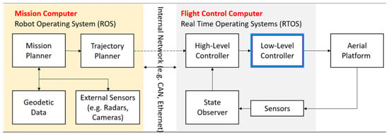
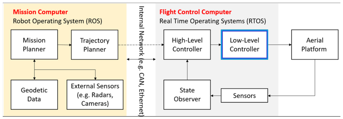
Each high-level algorithm implemented in Mission Computer (waypoint flight supervision) or Flight Computer (emergency handling) has a significant impact on the flight performance of the airborne platform. To verify the feasibility of the designed high-level algorithm, the system user must have access to the platform’s control algorithms via a SIL simulation system. The availability of SIL models developed for a specific platform is crucial for the designer of algorithms executed by an airborne platform’s Mission Computer, particularly one that operates autonomously and has no contact with the Ground Control Station (see Figure 1).
Figure 1.
A diagram of the Flight Computer (autopilot) and Mission Computer architecture. The method of exchanging flight plan information between the two computers is highlighted. The model simulates the Aerial Platform and Sensors, but the example shows a simplified Low-Level Component containing control models based on PID controllers.
The software presented in this article enables the development and testing of advanced control algorithms that account for the actual dynamics of a commercially available flying platform [2]. It allows simulating emergency and specific flight conditions that could cause the platform to crash in real-world situations. It enables a rapid transition from simulation to flight testing. The software was used in the design and testing of the flying platform described in [3]. If there is interest in the software, the repository (see Section 4) is planned to be expanded to include multi-rotor aircraft and VTOL hybrids.
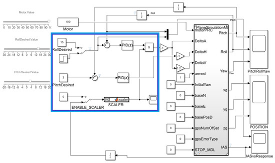
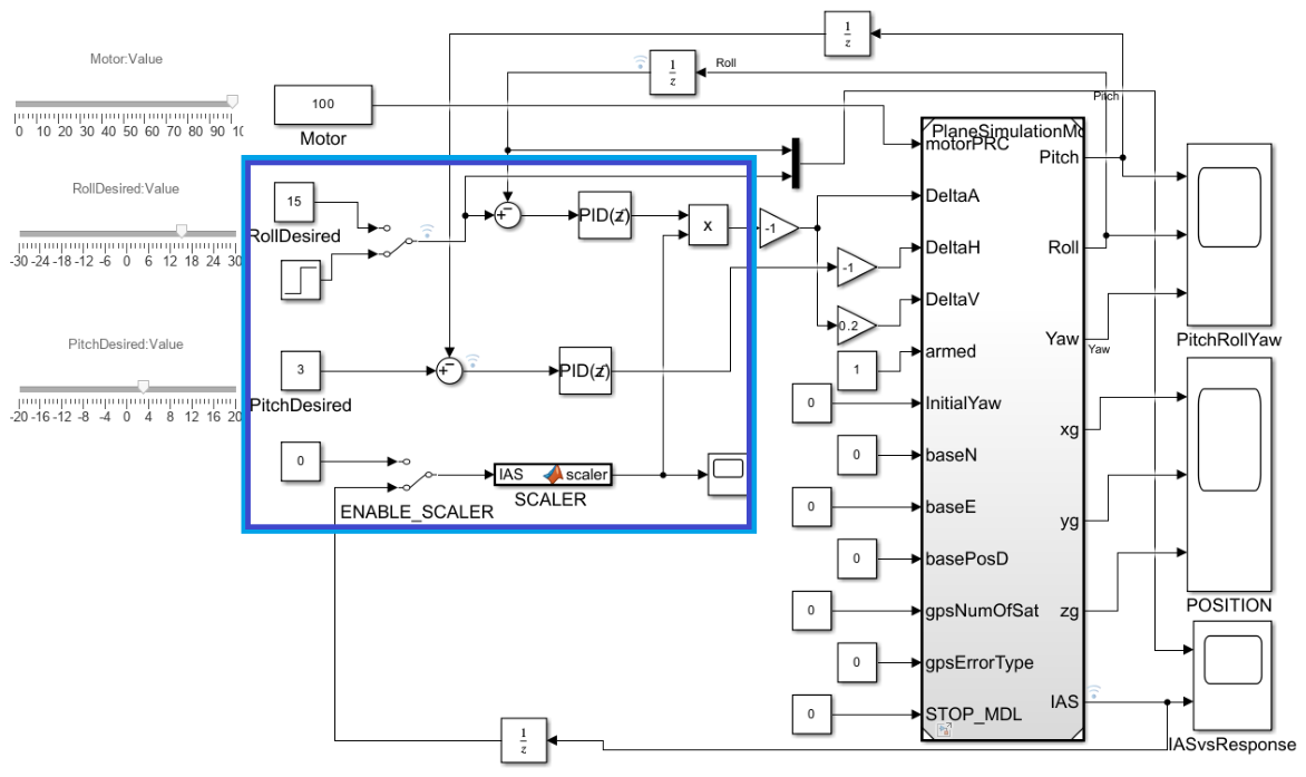
The software is implemented in a MATLAB/Simulink environment across several layers, with each subsequent layer providing greater detail. The top layer is a black box, where the inputs are specified by the pilot, such as engine speed and deflection of control surfaces, which generate the forces and moments that directly influence the UAV’s output state vector (see Figure 2).
Figure 2.
Main Software-In-the-Loop control panel. The pilot can specify the basic control values for UAV flight: pitch set value, roll set value, and motor PRC percent value. A simplified version of the autopilot Low-Level Controller is highlighted in blue.
In the simplest version, the user uses the top layer and can immediately start designing a Low-Level Controller (see Figure 1) using any algorithm (e.g., classical PID, LQR, sliding mode, backstepping, L1 control, etc.). The example in Section 5 shows a simplified Low-Level Component that stabilizes Pitch and Roll angles using PID controllers with an airspeed scaler.
The extended version allows connecting a physical autopilot with the Hardware Additional Blocks, such as ESC-ECL Blockset or https://www.mathworks.com/help/uav/px4/ug/px4-hitl-system-architecture.html (accessed on 8 April 2026).
The second example shows a connected autopilot using the ESC-ECL toolbox with real hardware and a Fighter UAV. Additionally, the user can connect a joystick and 3D visualization using other MATLAB/Simulink packages and perform a flight simulation (see Figure 2).
Kits for building fixed-wing aircraft are available on the civilian market. These kits include the airframe and its accessories, including servos, engines, and autopilots. Any user of such a system can purchase a pre-configured system ready for flight, as the autopilot comes with a preinstalled configuration for a specific platform type. However, if the user of such a system wishes to configure or design autopilot algorithms themselves, or to fly in manual control mode with limited autopilot supervision, a SIL simulation environment is required to introduce and verify defined constraints on UAV parameter control.
The developed software enables users with varying levels of experience in flight mechanics and aerodynamics to design and test UAV control algorithms in a SIL environment and in real flight using the Fighter UAV. Embedded aerodynamic models enable the user to simulate UAV operation without having to independently determine aerodynamic characteristics, a unique feature of the developed model. The problem of modeling the airframe’s dynamics based on the forces and moments acting on it was discussed by Chodnicki et al. [3].
The UAVConfigurator software implements all the necessary functions to simulate a real Fighter UAV. The example shown here illustrates a straightforward autopilot system designed to stabilize pitch and roll angles. The MATLAB/Simulink code is accessible at https://github.com/ESCSystems/UxV-Models (accessed on 1 April 2026).
The novelty presented in this work is the development of a SIL-class simulator for a COTS platform that incorporates aerodynamic models whose calculations are beyond the capabilities of users without in-depth knowledge of the system’s avionics. Thanks to the presented approach, system users can design their own UAV solutions incorporating advanced algorithms stored on the Mission Computer.
The rest of the article is as follows. Section 2 references the most important scientific studies available in the literature on this topic. Section 3 discusses key elements of the aerodynamics model of the described platform. Issues related to the construction of a UAV dynamics model, which relies on accurate calculations of forces and moments acting on the platform, are also presented. Section 4 describes the most important features of the built model (Section 4.1) and presents the system architecture in detail (Section 4.2). Section 5 demonstrates how to use the SIL simulator to design a custom solution for the Fighter platform. Section 6 discusses some of the issues air platform designers must consider when designing new solutions. Section 7 summarizes the results achieved.
2. Related Works
For fixed-wing UAVs, key performance parameters are influenced by aerodynamic factors. If the forces and moments acting on the platform are not accurately determined, catastrophic in-flight failures can occur, especially in unfavorable weather conditions. Therefore, this section primarily focuses on the challenges involved in calculating aerodynamic derivatives.
Most of the methods for determining aerodynamic derivatives presented in the vast body of literature on flight mechanics, which are required to analyze static and dynamic stability and to integrate aircraft equations of motion, are based on highly simplified engineering relations [4,5]. Typically, single values of derivatives are obtained, which are reasonably accurate within the linear range of the characteristics, which is usually the most important for aircraft basic performance analysis. This approach may be considered justified for a certain class of problems, especially those involving high Reynolds numbers and without flow separation effects. A common approach to solving such problems also relies on relatively simple computational aerodynamic methods, such as the vortex lattice method (VLM) [6,7] or potential (inviscid) panel methods [8], which more accurately account for effects like finite wingspan, wing planform, and non-planar aerodynamic configurations (e.g., biplane or wing–winglet layouts).
Cacciola et al. [9] present a procedure for determining flight mechanics models using multiple semi-empirical analyses implemented in a Digital DATCOM system to develop a flight mechanics model for fixed-wing unmanned aerial vehicles. The reference UAV selected to evaluate the proposed procedure is the Dragonfly DS-1, which is an electric vertical takeoff and landing UAV.
Other authors focus on selected elements of UAV aerodynamics. For example, Nikolaou et al. [10] describe unmanned platform winglet models that improve flight performance. Using surrogate-based optimization (SBO), winglet geometries with various geometric parameters, including roll and yaw angles, were developed. Li et al. [11] investigate the aerodynamic effects of rotors on fixed wings during the transition phase of foldable-wing unmanned aerial vehicles. In this type of UAV, during the transition from vertical takeoff to cruise, the rotor wake can be coupled to the fixed wing. Modeling aerodynamic changes allows us to determine the mode of flight-phase transition.
However, in the presence of phenomena that introduce nonlinearities, such as flow separation or formation of laminar separation bubbles (typically occurring at low Reynolds numbers, common in modern UAVs or gliders), such methods may prove significantly inadequate. Advanced flow analysis methods (CFD) (based on solving the Reynolds-averaged Navier–Stokes equations) may also be employed to compute aerodynamic derivatives by iteratively perturbing parameters such as angle of attack, side-slip angle, aircraft angular velocities, or control surface deflections, and subsequently determining the resulting changes in aerodynamic forces and moments. This approach yields significantly better-quality results, enabling the determination of derivatives over a range of angle-of-attack and airspeed values. However, it is computationally expensive, both in terms of mesh generation and in the computations themselves. It is also extremely challenging to account for issues such as the use of turbulators to trigger transition and prevent laminar separation—solutions commonly applied in light UAVs and gliders. In certain situations (particularly at low Reynolds numbers), the quality of contemporary computational methods, with respect to flow phenomena such as laminar–turbulent transition and laminar separation bubbles, still leaves considerable uncertainty about the reliability of the results. To improve accuracy, specific corrections based on wind tunnel testing can be applied, both static and dynamic, but access to such advanced data and analyses is greatly limited for many researchers.
The method presented in this work is based on flow analysis and the determination of aerodynamic characteristics using a panel method (the KK-AERO software package [12,13]) with strong inviscid flow and boundary–layer coupling. This software allows for relatively fast and labor-efficient determination of complete aerodynamic characteristics and derivatives, accounting for phenomena such as flow separation (up to the maximum lift condition), laminar boundary–layer instability and transition, laminar separation bubble formation, forced turbulent transition via turbulators, and control surface or flap deflections. It also enables the determination of hinge moments for simple, plain flaps and controls (without gaps or internal compensation). Without delving into the theoretical details of the method, it should be noted that the numerical scheme used in the above panel method (also known as the boundary element method) is based on an integral equation equivalent to solving the potential, linearized compressible flow Equation (the Prandtl–Glauert equation). The Kutta–Joukowski condition at the trailing-edge is formulated in a specific way. Unlike most similar methods, this is a nonlinear formulation that enforces equal pressures on the upper and lower surfaces of lifting surfaces at the trailing edge, where the vortex sheet begins. This formulation is presumably the most physically accurate for this condition, though it requires an iterative approach to solve the resulting nonlinear problem. Parabolic distributions of potential and linear or constant source distributions are used over quadrilateral elements (panels), which essentially ensures second-order accuracy of the method.
To account for viscous effects, two-dimensional boundary layer equations are applied in subsequent wing sections (the so-called strip method), generally consistent with the formulation used in the XFOIL program [14], which enables determination of 2D airfoil flow. Modifications include taking into account the “spreading” of streamlines (analogous to axisymmetric flow), and certain adjustments in modeling viscous dissipation in the wake and surface friction—changes that were selected to achieve the best agreement with experimental data [15,16,17]. The boundary layer is not calculated on non-lifting components of aircraft, such as the fuselage. The expected viscous drag of such elements must be specified externally. To reduce computational costs, the computational mesh is generated only for the basic aircraft geometry. Modifying boundary conditions model deflections of control surfaces and flaps on those surface segments. As a result, modified distributions of perturbation velocity potential are obtained, while the actual velocities, pressure distributions, and resulting aerodynamic forces and moments are determined on the actual, deformed surface. Numerous validated analyses (comparing results for real modified geometry with those based on simulated deflections) indicate that the error for practically relevant deflections is entirely acceptable, both in terms of pressure distributions and boundary–layer development, as well as in the resulting aerodynamic forces and moments. Using the same principle, aeroelastic deformation (wing bending and twisting) can also be incorporated. Ground effect, useful in analyzing aircraft takeoff and landing scenarios, can likewise be easily included.
3. Materials and Methods
This section presents a mathematical model for a fixed-wing UAV, specifically the commercially available Fighter UAV.
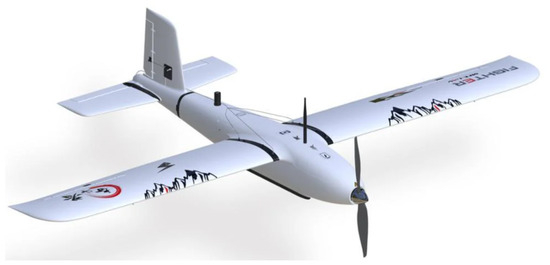
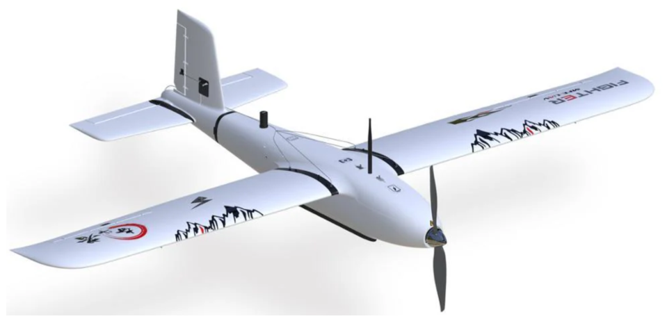
The first part of the section outlines a dynamics model based on the various forces and moments acting on the platform, as illustrated in Figure 3. The following section explains how these forces and moments are incorporated into the platform’s flight dynamics equations.
Figure 3.
Fighter UAV model: https://www.uavmodel.com/collections/fixed-wing-drone/products/makeflyeasy-striver-mini-binary-2100mm-uav-fixed-wing (accessed on 12 March 2026).
To use the developed MATLAB package to verify the operation of the Fighter platform, readers do not need to understand the model described in this section fully. The model is provided to clearly illustrate the approach to constructing simulators of this type for unmanned platforms.
The simplified mathematical model of the UAV is based on rigid-body dynamics and incorporates equations for the forces and moments acting on it. Newton’s second law of motion was used to determine the differential equations of the UAV’s kinematics and dynamics. To speed up the calculations, certain simplifications were made, omitting less important phenomena. First, it is assumed that the object is rigid, not deformable, of constant weight and constant inertia. Second, the center of mass is constant and does not change. This assumption is true for small UAVs equipped with electric motors. Third, the gravitational field is assumed to be uniform.
At the same time, it was assumed that all forces and moments acting on the platform must be expressed as equations derived from aerodynamic studies of the actual platform.
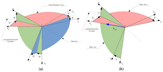
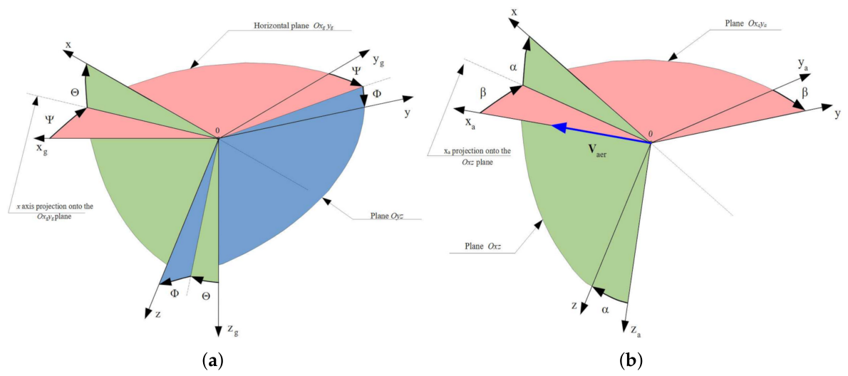
In modeling UAV dynamics, three coordinate systems are conventionally used, as shown in Figure 4, which denote: the Earth’s reference frame (), the UAV’s reference frame (), and the aerodynamic coordinate system ().
Figure 4.
(a) and frames of reference. (b) and frames of reference.
At the same time, transformation matrices between individual reference frames must be determined. depicts the transformation matrix between and , depicts the transformation matrix between and .
The parameter denotes the UAV yaw angle, describes the pitch angle, is the roll angle, is the UAV’s angle of attack, and is the UAV’s slip angle.
The UAV’s state vector is defined by the differential equations described below. These equations can be used to approximate the platform’s behavior, provided that the forces and moments acting on the platform are determined separately for each type of fixed-wing aircraft.
The derivatives of the angular speeds () in the body frame Oxyz are described as:
where:
- —moments that act on the object in the body frame (determining the moment values requires additional models shown later in the section).
- —moments of inertia of the UAV.
The derivatives of the linear velocities () are calculated in the reference frame .
where:
- —linear speeds in the body frame .
- —forces acting on the object in the body frame .
- m—mass of the UAV.
- —roll rate.
- —pitch rate.
- —yaw rate.
In the last step, the change in the position of the air platform is determined, which is defined by the system of equations:
where:
- —linear speeds in the body frame .
- —linear speeds in the Earth’s reference frame.
According to the above equations, the key to properly modeling aircraft dynamics is the correct determination of the forces and moments acting on the aircraft, as well as the mass-inertial parameters. Due to the complexity of determining complete aerodynamic derivatives for each platform type (which in practice involves determining the values of the coefficients (, , , , , ), the calculation principles are described in Section 2.
In this article, we use the results of these calculations, which were implemented in a simulation package shared on GitHub (see Section 4). Aerodynamic derivatives and dynamic pressure influence aerodynamic forces and moments:
where:
- .
- .
- .
- .
- —drag force (aerodynamic coordinate system).
- —lift force (aerodynamic coordinate system).
- —drag force (body frame).
- —side drag force (body frame).
- —lift force (body frame).
- L—roll moment (body frame).
- M—pitch moment (body frame).
- N—yaw moment (body frame).
Often, in modeling unmanned aircraft, especially low-cost ones, aerodynamics are significantly simplified, and autopilot tuning is performed experimentally during flight tests (see [18]). Given the similarity of the models and the information available online about initial settings and auto-tuning functions, the aircraft can usually be tuned for the given flight conditions. However, this approach does not allow for determining the aircraft’s behavior during flight under different environmental conditions, with different flight profiles, or with different dynamic constraints on the autopilot. The absence of an accurate model prevents the identification of platform limitations and the recognition of hazardous conditions in controlled environments.
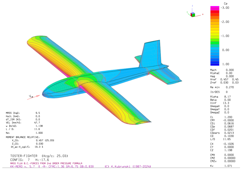
The Fighter UAV platform was tested in flight during various flight profiles and scenarios. In one flight, the platform became uncontrollable (risking destruction), especially at higher speeds. Therefore, additional aerodynamic analyses were performed (see Figure 5 and Figure 6). For aerodynamic calculations, we used the proprietary software KK-AERO (version 1.1), developed by one of the authors of the article (cited in [12,13]). The effectiveness and quality of this software have been validated in the literature (see [19,20]) as well as in the design of flying aircraft structures, including the world-class Diana-2 glider https://pl.wikipedia.org/wiki/SZD-56_Diana (accessed on 12 March 2026).
Figure 5.
Fighter UAV pressure distribution.
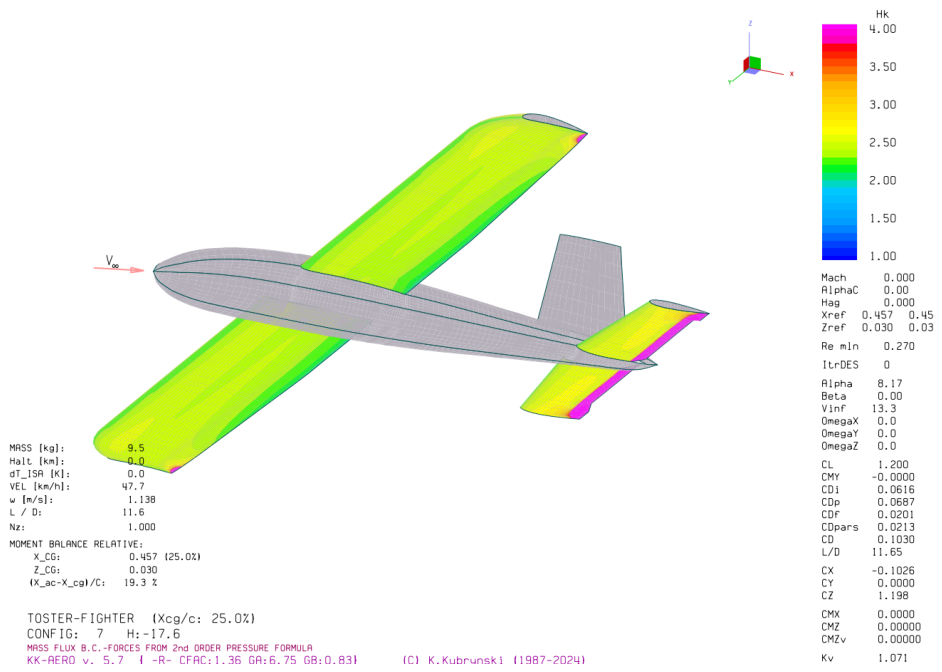
Figure 6.
Fighter UAV shape parameter .
The result of the calculations is a matrix under equilibrium conditions. Trim conditions depend on (, , ) with fixed airflow speed. The results are available in the repository, and part of the table is shown in Table 1.
Table 1.
Aerodynamic derivatives per [rad] with trim conditions for ,,. Only a subset is shown here, with the full dataset provided in the repository (see Section 4).
The simulation software uses current results to interpolate between equilibrium points. With additional programming, it enables smooth transitions between operating points, which is essential for preventing peaks during calculations, which would be significantly amplified, particularly in the derivative control terms.
The applied aerodynamic calculation method accounts for the interaction between the actual, full geometry and its elements; therefore, there is no need to use approximate relationships that introduce imprecise corrections.
For example, the contribution of the vertical tail to the derivative of for the applied approach automatically takes into account the influence of the fuselage on increasing the lateral angle of inflow onto the tail, which is crucial compared to commonly used simplified methods [21] (including those used in AVL, Aerospace Toolbox) and simulation tools (Xplane, Ardupilot SITL), especially aerodynamic, is simplified with Multirotor solutions/projects [22,23]. In addition to simplified aerodynamic calculations, these programs often do not account for variable operating points, assuming constant coefficients regardless of current flight parameters.
Additionally, most examples in MATLAB/Simulink refer to the aerodynamics of well-known, large, and untestable aircraft, such as the Cessna. This feature is another advantage of our model, which has been made available, in that it reflects publicly available real-world UAV models.
PX4/Ardupilot SITL/HITL is a repository in the GitHub ardupilot where one can find the implementation of the plane simulator. At the top of the file (https://github.com/ArduPilot/ardupilot/blob/master/libraries/SITL/SIM_Plane.cpp) (accessed on 4 May 2026), one can find that this is a very simple plane simulator class, not aerodynamically accurate, just enough to be able to debug control logic for new frame types. This simulator is not designed to tune or check the behavior of advanced control algorithms. It is simply used to check the logic of Ardupilot functionality. The Xplane simulator is more accurate than the Ardupilot SITL and allows for preliminary adjustments of controller settings. However, it is a closed, commercial solution, making it impossible to precisely assess its accuracy. However, the available SDKs and descriptions indicate that its aerodynamics are also calculated from an engineering perspective and contain significant simplifications, particularly ignoring the impact of wing–fuselage interactions, which can be found in materials on the Xplane forum (forums.x-plane.org). Comparison of SIL/HIL simulators is presented in Table 2.
Table 2.
Comparison of popular SIL/HIL autopilot simulators.
The detailed expansion of the aerodynamic derivatives used, along with their dependencies on the current state vector and control, is shown below.
where:
Initial values:
—reference span (for Fighter UAV = 2.43 m).
—reference chord (for Fighter UAV = 0.2977 m).
—reference area (for Fighter UAV = 0.721 sq m).
m—weight (for Fighter UAV assumed 9.5 kg).
Aerodynamic coefficients (Table 1):
—frontal drag force coefficient.
—lateral resistance force coefficient.
—lift coefficient.
—roll moment coefficient.
—pitching moment coefficient.
—yaw moment coefficient.
—angle of attack for trim condition.
—horizontal deflection angle (elevator) for trim conditions.
—flap deflection angle for trim conditions.
State vector parameters (Equation (13)):
—current angle of attack.
—current sideslip angle.
p, q, r—current angular rates.
—current aerodynamic speed.
—current vertical acceleration.
Control signals (Section 4.2):
—current aileron deflection angle.
—current horizontal (elevator) deflection angle.
—current vertical (rudder) deflection angle.
—current flap deflection angle (not present in Fighter UAV).
We refer the reader to other works (see [24,25,26]) that describe the principles of modeling and simulation of aerial platforms, where basic models of platform dynamics are presented. An advanced UAV simulation environment was also presented by Dai [27].
The red color in Figure 6 represents a high value of the kinematic shape parameter and flow separation (in the form of laminar separation bubbles or turbulent boundary layer at the trailing edge). It is worth noting that in a clean, horizontal tail configuration, the laminar boundary layer undergoes strong flow separation, leading to strong nonlinearities. Applying turbulators (see description [28]) on both surfaces, there are no separations and many linear characteristics.
This case demonstrates the need for accurate modeling of aircraft dynamics, including complete aerodynamics. The approach presented here demonstrates the methodology and model preparation method. This approach becomes crucial for larger, faster, and, above all, expensive platforms, or for systems with limited real-world testing capabilities, particularly when the aircraft’s dynamic parameters change during flight, requiring the Low-Level Controller to use different algorithms or control settings for each flight phase.
The aerodynamic identification of the object, including its derivatives and coefficients defined by Equations (14)–(21), is shown in detail below, and the derivative table has been placed in the repository along with the model.
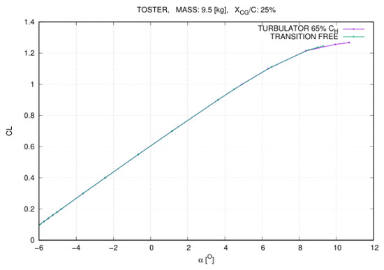
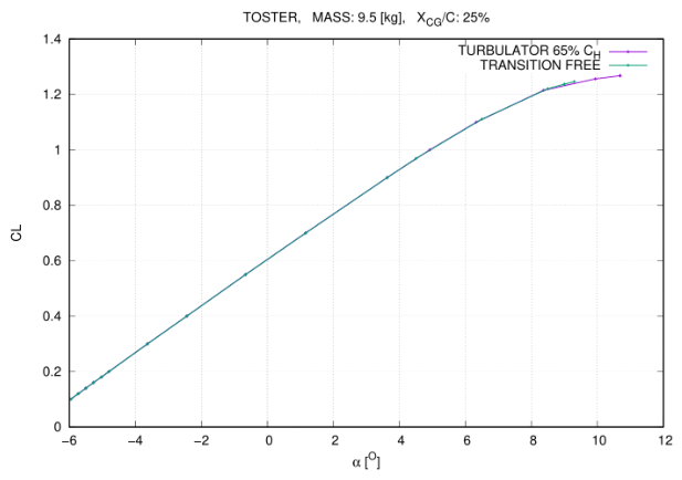
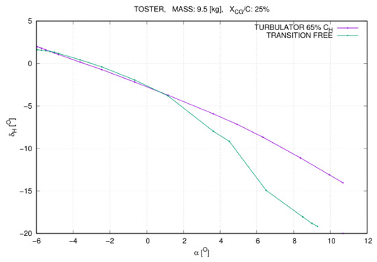
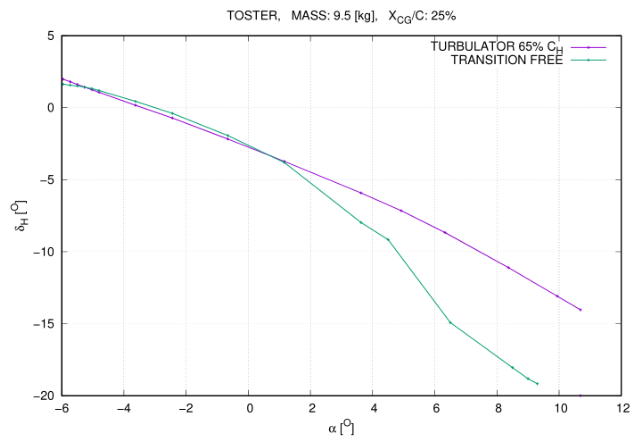
Figure 7 and Figure 8 present calculated lift characteristics () and required elevator deflection angle () to preserve longitudinal trim of the above airplane for the case of clean configuration (Figure 7) and with a turbulator on both sides of the horizontal surface. Strong nonlinearities are evident in the free transition case. At high angles of attack, there exists flow separation on the lower surface of the elevator, while at high speeds (low angles of attack), there is flow separation on the upper side of the elevator (in the form of quite long separation bubbles).
Figure 7.
Calculated lift characteristic in case of free and forced transition (via turbulator).
Figure 8.
Elevator deflection for trim in case of free and forced transition (via turbulator).
Aerodynamic derivatives are determined by establishing equilibrium conditions (elevator deflection) for a given center of gravity location, and subsequently perturbing parameters such as angle of attack, side-slip angle, angular velocities, or control surface and flap deflections. The aerodynamic derivatives are calculated using finite differences with a first-order or second-order (central) scheme. The only remaining challenge is the determination of the derivative with respect to the rate of change of angle of attack (or equivalently, vertical acceleration)—these are unsteady derivatives by nature, reflecting mainly the lag in the influence of wing lift changes on the force generated on the horizontal tail (in the case of conventional configurations). The solution to this problem is based on a classical analytical approach, involving the calculation of the ratio of the tail angle-of-attack deviation to the aircraft angle of attack. This is a two-step process. In the first one, the derivative is determined using a somewhat unorthodox approach: the angle of attack is perturbed, and the horizontal tail surface (treated as a all-moving tailplane) is deflected by an amount that produce the same total force on the horizontal tail as before—meaning the same local tail angle of attack with respect to the flow at the tail’s location. The final values of derivatives with respect to are then obtained from the relation [15]:
The generated forces and moments are significantly influenced by aerodynamic speed. Consequently, wind and turbulence parameters play a crucial role in determining the energy demands for a flight that meets specified criteria.
4. Software Description
The section describes the fundamental elements of the SIL architecture, enabling users of the Fighter UAV system to independently parameterize specific system components (Table 3).
Table 3.
MATLAB/Simulink code metadata.
4.1. Software Functionalities
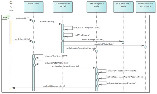
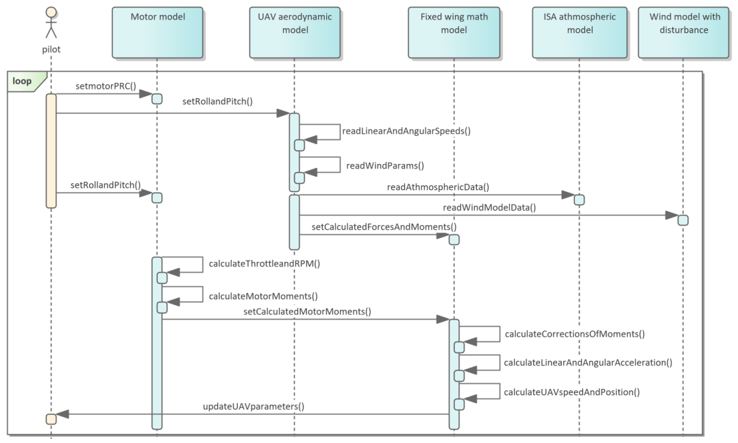
The basic functionality of the developed software involves updating the UAV’s position in flight based on settings entered by the UAV pilot in manual mode. The operating scenario is shown in Figure 9 as a UML sequence diagram.
Figure 9.
Schematic diagram of the UAV position calculation process in UML.
During the flight, every predetermined segment, , the SIL reads the pilot-defined settings (engine power, UAV roll, and yaw). The engine model determines the RPM and throttle position. Data on atmospheric and wind parameters are collected. The moments acting on the UAV (which depend directly on the engine type, pilot settings, and the UAV’s roll and yaw angles) are determined from the engine simulator. The forces acting on the UAV are determined from the UAV’s aerodynamic model (specific to the airframe), and the moments from the engine model are corrected. These values require data on the UAV’s speed and yaw angle, wind parameters, and pilot-defined settings.
The calculated force and moment values, along with current telemetry data, constitute input to the UAV’s mathematical model, described in detail in [3]. The model’s output calculates linear and angular accelerations, along with changes in the UAV’s roll and pitch, which affect its current position.
The output from these models can be used to model real-world devices that influence UAV sensors, such as IMU, GPS/GNSS, or magnetometers.
4.2. Software Architecture
4.2.1. Pilot Control Panel
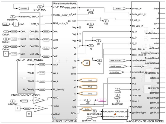
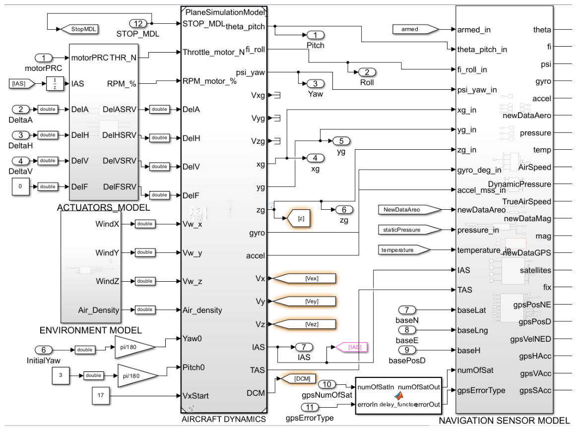
The pilot enters four variable values on the SIL model’s control panel: the engine control level [0–100%], which is set during flight (input “motorPRC”), the aircraft’s elevator (input “DeltaH”), aileron (input “DeltaA”), and rudder (input “DeltaV”). The remaining values (atmospheric and wind parameters) are retrieved from the appropriate models (see Figure 10). The UAV model’s input also includes basic values obtained from the UAV telemetry, such as the current roll, pitch, and yaw angles, linear and angular speeds, and linear and angular accelerations (see [3]), required to calculate the UAV’s position.
Figure 10.
Software-In-the-Loop architecture. SIL consists of components: PlaneSimulationModel, Motor simulation, Atmospheric model, wind with turbulence model.
4.2.2. Plane Simulation Model
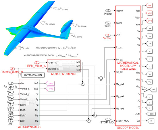
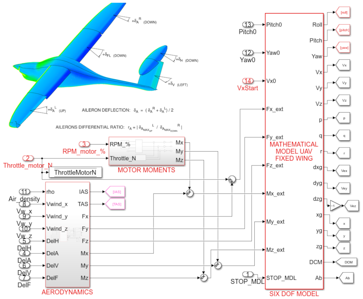
The airframe simulation model (see Figure 11) consists of two main parts: a mathematical model of the UAV that accounts for the forces and moments acting on it in flight, and a model that determines these forces and moments using aerodynamic models. The aerodynamic models are enhanced by incorporating detailed representations of engine and servomechanism operations.
Figure 11.
A plane simulation model consisting of two main parts: the UAV aerodynamics component and the mathematical model of the UAV. Aerodynamics and Motor components calculate forces and moments acting on the UAV. The 6-DOF mathematical model updates the UAV’s position at each time step.
The aerodynamic model is a unique package developed as part of the project and published in this publication. Determining flight parameters solely from moments and forces acting on the UAV does not allow for controlling the airframe in real-world situations, as the interdependencies among parameters are not accounted for. Therefore, providing a complete model of the actual platform is crucial.
4.2.3. Engine Simulation Component
SIL uses a simplified model of the UAV’s electric motor with a propeller. The MOTOR MOMENTS component determines the moments acting on the UAV: the gyroscopic and engine moments. The model’s input data are the UAV’s speed and the pilot-specified RPM as a percentage of the engine’s total power. The output provides moments in each of the three flight axes.
4.2.4. ISA Atmosphere and Wind Simulation Component
The ISA atmosphere and wind simulation components model the effects of atmospheric conditions on UAV flight, serving as the environmental framework for each model. The wind and turbulence model is now finalized and can be implemented using the Dryden model (refer to [29]), which is available in MATLAB. The software employs an atmospheric model that lacks turbulence modeling.
4.2.5. Model of On-Board Equipment
The system model includes simplified blocks to simulate interference from on-board components affecting UAV flight. These blocks are located in the NAVIGATION SENSOR MODEL block (see Figure 10). These primarily include IMU, GPS, and magnetometer models. The model’s input is a set of state vector parameters, including the UAV’s current position and the number of satellites from which the GPS receives data, provided by the user. The output is the UAV’s position, corrected for vertical and horizontal deviation errors and GPS latency, in WGS84 format. Sensor models are available in the MATLAB package [30].
5. Illustrative Example
5.1. Example 1—SIL Simulation
The aircraft is controlled using variables corresponding to the actual control (see Figure 2): motorPRC (engine control in the range of 0–100%), aileron, elevator, and rudder deflection (DelA, DelH, and DelV in the range of ±15 degrees).
Example test_r17 in the GitHub repository demonstrates the design and validation of an autopilot system for pitch and roll angle control, and examines the effect of scaling control signals as a function of airspeed. This scaling, both in reality and in the example simulation, is implemented via feedback from a dynamic pressure sensor. The example demonstrates research that enables the assessment of flight safety when scaling is not possible, for example, in the event of sensor damage during flight due to issues with electrical, pneumatic, or electronic systems. This test is critical for aircraft operating at high speeds from a safety perspective.
Simplified stabilization was achieved using two PID controllers and aileron and rudder feedforward commands (DelV) with a constant gain of 0.2 (see Figure 2). The pitch channel can be adjusted with a slider; however, in this example, the pitch angle was maintained at 3 degrees.
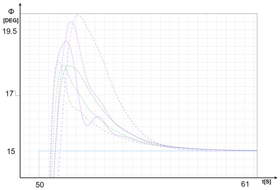
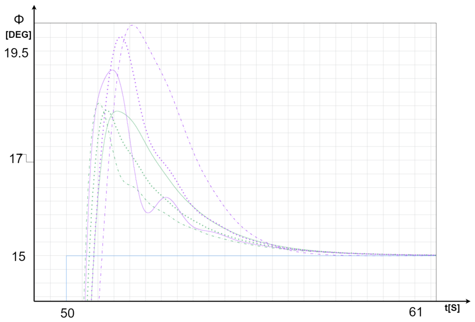
This example demonstrates how the step response of the roll channel changes over time, stabilizing the angle depending on the scaling parameters used.
Each test case was conducted with a single 15-degree roll over a simulation period of 50 s (as shown by the blue line in Figure 12). The scaling block values were adjusted in three ways: disabled (resulting in an output value of 1), with the linear variant enabled, and with the quadratic variant enabled. In addition, the engine control value was increased from 70% to 100%, corresponding to a flight speed of approximately 17 m/s at the minimum and about 29 m/s at the maximum for the aircraft.
Figure 12.
Values of the step response of roll control for the described cases: 1. Scaler off and motor controlled at approximately 70% ( purple graph); 2. Scaler off and motor controlled at approximately 100% ( green graph); 3. Scaler on, linear variant, and motor controlled at approximately 70% (… purple graph); 4. Scaler on, linear variant, and motor controlled at approximately 100% (… green graph); 5. Scaler on, quadratic variant, and motor controlled at approximately 70% (− purple graph); 6. Scaler on, quadratic variant, and motor controlled at approximately 100% (− green graph).
The results should be interpreted as follows. Firstly, the tested aircraft remains stable regardless of the applied scaling. Secondly, with the current PID controller settings, the scaler helps to align the step response signals at different speeds more closely. Among the scalers tested, the quadratic scaler produced the best results, as evidenced by the continuous purple and green graphs being similar. In contrast, when the dash-dot scaler was disabled, the overshoot values and settling times were significantly different.
The example provided serves as a foundation for developing and testing aircraft dynamics. Using MATLAB/Simulink and additional tools such as ESC Embedded Coder Lab [31], we can run the developed algorithms on a real aircraft and conduct flight tests without writing any C code.
5.2. Example 2—HIL Simulation
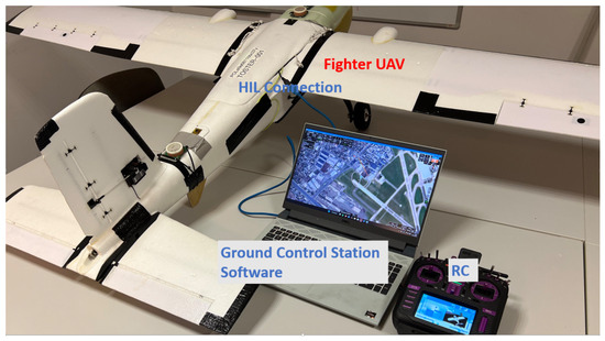
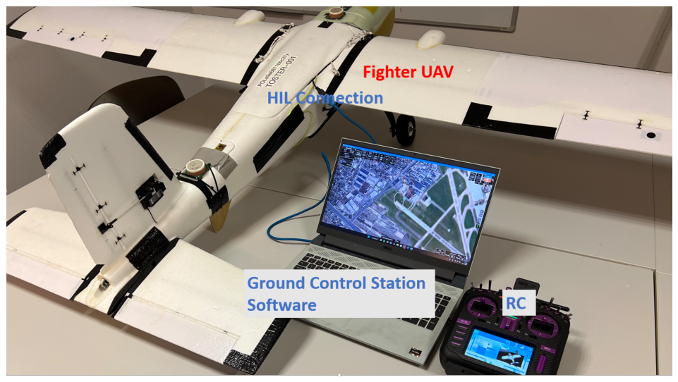
The model described in Section 3 and Section 4 was integrated with the ESCsystems production control system (see [31]) via the ESC Embedded Coder Lab, enabling pre-flight testing using the Hardware-In-the-Loop (HIL) method. The simulation environment is illustrated in Figure 13. HIL testing can also be conducted with other open-source control systems, such as UAV autopilots and third-party platforms. When simulating the operation of a different platform, the aircraft’s physical parameters in the model need to be adjusted to facilitate testing for that specific platform. HIL simulation models for realistic drone or drone swarm control are becoming increasingly common in the literature (e.g., [32,33]). The systems typically integrate physical control modules with SIL simulation.
Figure 13.
Fighter simulation set in HIL configuration with GCS ground control station software (ver.1.0).
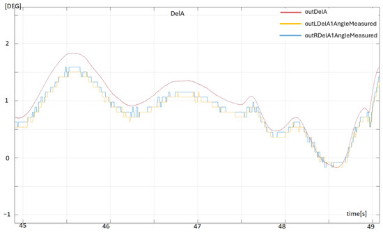
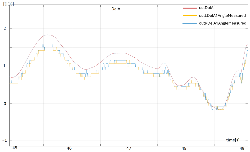
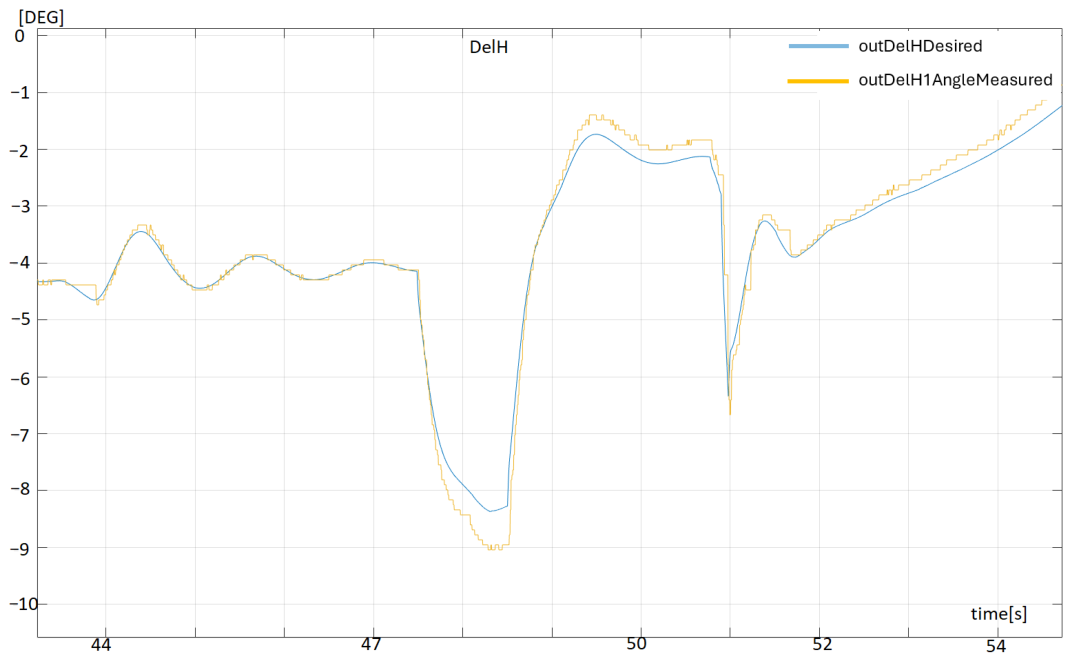
During HIL testing, we conducted a series of simulations and unit tests of the complete system. These tests enabled the UAV operator to verify communication between the Ground Control Station (GCS) and the platform, practice the planned flight scenarios for upcoming flight tests, and ensure proper control of the actuators during maneuvers commanded by the GCS. This paper presents the variations in aileron deflection (see Figure 14) and elevator deflection (see Figure 15) values determined by the autopilot, as well as their physical processing by the servos.
Figure 14.
Changes in the set aileron deflection angle and the values read from the left and right aileron servos.
Figure 15.
Adjustments to the set angle of elevator deflection and the corresponding values obtained from the servos.
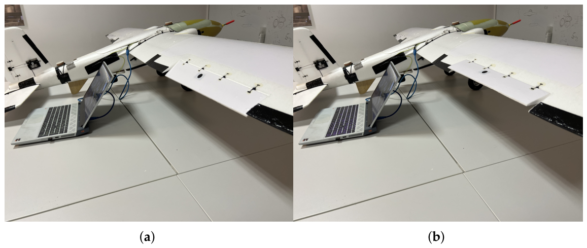
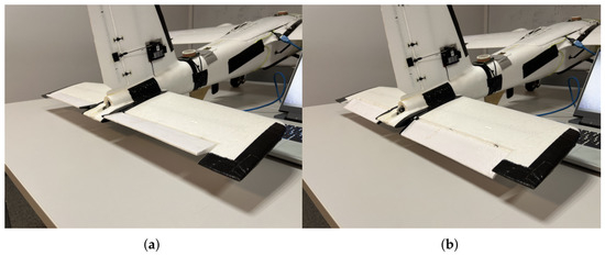
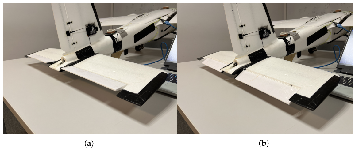
During HIL tests, we evaluate the actuators’ angle calculation accuracy based on several factors, including deflection direction, response speed, transfer frequency, and the absence of oscillation. To verify the tailplane’s performance during flight, we utilize artificial loads. The evaluation results are illustrated in Figure 14 and Figure 15, while visual observations of the aircraft are presented in Figure 16 and Figure 17.
Figure 16.
Aileron deflections: (a) when making a left turn, (b) when making a right turn. The photo shows the Fighter platform integrated with a flight simulator.
Figure 17.
Elevator deflections: (a) during upward flight (b) during descent.
During testing, based on the plots in Figure 14 and Figure 15, it is possible to verify the correctness of the response and the actual deflections of the servomechanisms to the control signals generated by the autopilot system. The plots show differences in signal amplitude, transmission frequency, and sampling rate. All of the above data are logged during flight tests and serve as the basis for model verification and validation.
Figure 16 and Figure 17 show selected extreme positions in response to the commanded flight phases, which is a key pre-flight verification step for both manual and automatic flight operations. It may happen that the pilot has incorrectly set the reverse directions on the control sticks, and in combination with the autopilot settings, the entire system must still produce deflections consistent with the aerodynamic control system.
6. Discussion
The provided software, combined with MATLAB Coder, Simulink Coder, and hardware support packages for STM32 microcontrollers, such as ESC Embedded Coder Lab, allows for the direct transfer of algorithms from the simulation environment to physical hardware and perform HIL tests. Algorithms developed and tested in SIL can be readily and quickly tested in real-world environments using the relatively inexpensive Fighter UAV research platform. Such a widespread and accessible platform enables the verification and comparison of published control and navigation algorithm results not only in simulation but also in real-world environments internationally. All tests were executed in MATLAB 2023b on a computer equipped with an Intel Core i7 processor.
The software is open-source and provides an excellent basis for aircraft simulation and design, for example, for SAE Aero Design competitions. Thanks to MATLAB/Simulink tools, the solution can be used to develop anti-collision algorithms, verify constraints, work in swarms, and more. The main task of the software is to enable easy, almost direct transition from simulation tests to flight tests.
The literature provides numerous implementations of aircraft, including unmanned aircraft. However, the aerodynamic and control coefficients chosen are often empirical and not specific to a particular aircraft. The available software, combined with reliable aerodynamic calculations (unavailable in most UAV studies) and subsequent flight tests, enables the implementation of the developed algorithms.
UAVConfigurator software is expected to become a tool for users who prefer manual flights to configure their own unmanned platform solutions. The designed application can be extended to other commercially available unmanned systems, requiring only the development of appropriate models to calculate the forces and moments acting on the platform as a function of specific control variables.
The software was developed as a result of research and development during larger projects. To make the selected component available, we decided to adapt it to a publicly available airborne platform. Combined with another commercial ESC ECL tool [31], it enables fully automated code generation for STM32 microcontroller-based systems, HIL testing, and the design of advanced control solutions.
The commercial license for the software built on UAVConfigurator enables a designer to develop their own advanced UAV solutions. The academic license allows the design of systems for research purposes.
The presented software has been successfully verified for use in classified projects, primarily for military purposes. A commercial platform was chosen in this article so that the method could be made public, allowing the scientific community and others to validate it in their projects and research. Performed flight tests demonstrated in the attached movie that no modifications to the controller settings were needed after they were tuned in the HIL environment.
Detailed validation and verification of the flight tests will be the subject of a subsequent article. This article aimed to provide a publicly available tool for testing algorithms on an off-the-shelf test aircraft.
7. Conclusions
The SIL-class model presented in this article enables the verification of the developed platform control method while simultaneously enhancing flight safety. The software’s uniqueness is highlighted by its incorporation of an aerodynamic model of a real commercial aircraft, which facilitates the transition from pilot-input forces to the forces and moments acting on the platform. The model primarily uses formal methods to determine aerodynamic coefficients, which are rarely reported in the literature because they are derived for specific aircraft models, and the process is computationally intensive. This modeling method provides a realistic flight simulation experience. An approach utilizing SIL and HIL simulations not only accelerates the design process but also reduces associated costs.
Author Contributions
Conceptualization, M.C. and W.S.; methodology, M.C. and K.K.; software, M.C.; validation, M.C., W.S. and K.K.; formal analysis, K.K.; resources, M.C.; writing—original draft preparation, M.C. and W.S. All authors have read and agreed to the published version of the manuscript.
Funding
This research was financed as part of an internal R&D project at AFIT.
Institutional Review Board Statement
Not applicable.
Informed Consent Statement
Not applicable.
Data Availability Statement
The MATLAB project and the data used for the simulation are available on Github (https://github.com/ESCSystems/UxV-Models, accessed on 11 May 2026).
Conflicts of Interest
The authors declare no conflicts of interest.
Abbreviations
The following abbreviations are used in this manuscript:
| UAV | Unmanned Aerial Vehicle |
| SIL | Software-In-the-Loop |
| HIL | Hardware-In-the-Loop |
| PID | Proportional Integral Derivative regulator |
| LQR | Linear-quadratic regulator |
| DOF | Degrees of Freedom |
| COTS | Commercial Off-The-Shelf |
| IMU | Inertial Measurement Unit |
| GPS | Global Positioning System |
| GNSS | Global Navigation Satellite System |
| RTOS | Real-Time Operating System |
| ROS | Robot Operating System |
References
- Chen, L.; Liu, Z.; Dang, Q.; Zhao, W.; Chen, W. Robust fixed-time flight controller for a dual-system convertible UAV in the cruise mode. Def. Technol. 2024, 39, 53–66. [Google Scholar] [CrossRef] [Scilit]
- Fighter UAV System Description. 2026. Available online: https://rcdrone.top/products/makeflyeasy-fighter-2430mm-mfe-fighter-vtol (accessed on 13 January 2026).
- Chodnicki, M.; Siemiatkowska, B.; Stecz, W.; Stepien, S. Energy Efficient UAV Flight Control Method in an Environment with Obstacles and Gusts of Wind. Energies 2022, 15, 3730. [Google Scholar] [CrossRef] [Scilit]
- Fink, R. USAF Stability and Control DATCOM, AFWAL-TR-83-3048; Flight Dynamics Laboratory, Air Force Aeronautical Laboratories, Air Force System Command, Wright-Patterson AFB: Dayton, OH, USA, 1978. [Google Scholar]
- Smetana, F.O.; Summey, D.C.; Johnson, W.D. Riding and Handling Qualities of Light Aircraft—A Review and Analysis; NASA CR-1975; National Aeronautics and Space Administration: Washington, DC, USA, 1972. [Google Scholar]
- Kay, J.; Mason, W.H.; Durham, W.; Lutze, F.; Benoliel, A. Control Authority Issues in Aircraft Conceptual Design: Critical Conditions, Estimation Methodology, Spreadsheet Assessment, Trim and Bibliography; VPI-Aero-200, (Minor Revisions 1996); Department of Aerospace and Ocean Engineering, Virginia Polytechnic Institute and State University: Blacksburg, VA, USA, 1993; Available online: https://scispace.com/pdf/control-authority-issues-in-aircraft-conceptual-design-26aaqc3sga.pdf (accessed on 1 April 2026).
- Drela, M.; Youngren, H. AVL Software (Athena Vortex Lattice), 1988–2017. Available online: https://web.mit.edu/drela/Public/web/avl/ (accessed on 1 April 2026).
- Goetzendorf-Grabowski, T. PANUKL2024—Package to Compute the Aerodynamic Characteristics of an Aircraft Using Low Order Panel Method. Available online: https://www.meil.pw.edu.pl/add/ADD/Teaching/Software/PANUKL (accessed on 1 April 2026).
- Cacciola, S.; Testa, L.; Saponi, M. A Procedure for Developing a Flight Mechanics Model of a Three-Surface Drone Using Semi-Empirical Methods. Aerospace 2025, 12, 515. [Google Scholar] [CrossRef] [Scilit]
- Nikolaou, E.; Kilimtzidis, S.; Kostopoulos, V. Winglet Design for Aerodynamic and Performance Optimization of UAVs via Surrogate Modeling. Aerospace 2025, 12, 36. [Google Scholar] [CrossRef] [Scilit]
- Ai, L.; Xia, H.; Yang, J.; He, Y.; Tang, W.; Fan, M.; Xiang, J. A Study on the Aerodynamic Impact of Rotors on Fixed Wings During the Transition Phase in Compound-Wing UAVs. Aerospace 2024, 11, 945. [Google Scholar] [CrossRef] [Scilit]
- Kubrynski, K. Design of 3-Dimensional Complex Airplane Configurations with Specified Pressure Distribution via Optimization. In Proceedings of the ICIDES-III Conference, Washington, DC, USA, 23–25 October 1991; Dulikravich, G.S., Ed.; Pennsylvania State University: University Park, PA, USA, 1991; pp. 263–280. Available online: https://ntrs.nasa.gov/api/citations/19920004730/downloads/19920004730.pdf (accessed on 2 May 2026).
- Kubrynski, K. Subsonic Aerodynamic Design via Optimization. In Recent Development of Aerodynamic Design Methodologies—Inverse Design and Optimization; Fuji, K., Dulikravich, G.S., Eds.; Notes on Numerical Fluid Mechanics; Vieweg+Teubner Verlag: Wiesbaden, Germany, 1999; Volume 68. [Google Scholar] [CrossRef] [Scilit]
- Drela, M. XFOIL: An Analysis and Design System for Low Reynolds Number Airfoils. In Low Reynolds Number Aerodynamics; Mueller, T.J., Ed.; Lecture Notes in Engineering; Springer: Berlin/Heidelberg, Germany, 1989; Volume 54. [Google Scholar] [CrossRef] [Scilit]
- van Rooij, R.P.J.O.M. Modification of the Boundary Layer Calculation in RFOIL for Improved Airfoil Stall Prediction; Report IW-96087R; Institute for Wind Energy, Delft University of Technology: Delft, The Netherlands, 1996. [Google Scholar]
- Kubrynski, K. Design of a Flapped Laminar Airfoil for High Performance Sailplane. In Proceedings of the 30’th AIAA Applied Aerodynamics Conference, New Orleans, LA, USA, 25–28 June 2012; AIAA Paper 12-2662. 20pAvailable online: https://www.researchgate.net/profile/Krzysztof-Kubrynski/publication/268562382_Design_of_a_Flapped_Laminar_Airfoil_for_High_Performance_Sailplane/links/56e026e208ae9b93f79c253c/Design-of-a-Flapped-Laminar-Airfoil-for-High-Performance-Sailplane.pdf (accessed on 2 May 2026).
- Hansen, T. Airfoil Optimization for Wind Turbine Application. Wind Energy 2017, 21, 461–603. [Google Scholar] [CrossRef] [Scilit]
- Etkin, B.; Reid, L.D. Dynamics of Flight, Stability and Control, 3rd ed.; Wiley & Sons: Hoboken, NJ, USA, 1996. [Google Scholar]
- Boermans, L.M.M.; Nicolosi, F.; Kubrynski, K. Aerodynamic Design of High-Performance Sailplane Wing-Fuselage Combinations. In Proceedings of the 21st Congress of International Council of the Aeronautical Sciences, Melbourne, VIC, Australia, 13–18 September 1998; Paper ICAS-98-2.9.2. Available online: https://www.icas.org/icas_archive/ICAS1998/PAPERS/292.PDF (accessed on 8 April 2026).
- Kubrynski, K. High Performance Sailplane Design Strategy Using Inverse Design and Optimization Techniques. In Proceedings of the Inverse Problems, Design and Optimization, IPDO-2007, Miami, FL, USA, 16–18 April 2007; Available online: https://www.researchgate.net/publication/309209815_HIGH_PERFORMANCE_SAILPLANE_DESIGN_STRATEGY_USING_INVERSE_DESIGN_AND_OPTIMIZATION_TECHNIQUES (accessed on 2 May 2026).
- Shen, T.-J.; Chen, C.-L. Model-in-the-Loop Design and Flight Test Validation of Flight Control Laws for a Small Fixed-Wing UAV. Drones 2025, 9, 624. [Google Scholar] [CrossRef] [Scilit]
- Santos, M.A.; Becker, L.B.; Esteban, S.; Raffo, G.V. ProVANT Simulator: A Virtual Unmanned Aerial Vehicle Platform for Control System Development. Aerospace 2025, 12, 762. [Google Scholar] [CrossRef] [Scilit]
- Welcer, M.; Sahbon, N.; Zajdel, A. Comparison of Flight Parameters in SIL Simulation Using Commercial Autopilots and X-Plane Simulator for Multi-Rotor Models. Aerospace 2024, 11, 205. [Google Scholar] [CrossRef] [Scilit]
- Silva, W.R.; da Silva, A.L.; Gründling, H.A. Modeling, simulationand control of fixed-wing unmanned aerial vehicle (UAV). In Proceedings of the 24th ABCM International Congress of Mechanical Engineering, Curitiba, Brazil, 3–8 December 2017. [Google Scholar]
- Noureldein, A.; Zakaria, M.; Kamal, A.M. Investigating Tailless UAV Flight Dynamics through Modeling, Simulation, and Flight Testing. Unmanned Syst. 2025, 13, 455–475. [Google Scholar] [CrossRef] [Scilit]
- D’antuono, V.; De Matteis, G.; Trotta, D.; Zavoli, A. Optimization of UAV Robust Control Using Genetic Algorithm. IEEE Access 2023, 11, 122252–122272. [Google Scholar] [CrossRef] [Scilit]
- Dai, X.; Ke, C.; Quan, Q.; Cai, K.-Y. RFlySim: Automatic test platform for UAV autopilot systems with FPGA-based hardware-in-the-loop simulations. Aerosp. Sci. Technol. 2021, 114, 106727. [Google Scholar] [CrossRef] [Scilit]
- WingWheels, Zig Zag & Dimple Turbulator. 2026. Available online: https://wingsandwheels.com/zig-zag-turbulator-dimple-tape.html (accessed on 13 January 2026).
- Liepmann, H.W. On the Application of Statistical Concepts to the Buffeting Problem. J. Aeronaut. Sci. 1952, 19, 793–800. [Google Scholar] [CrossRef] [Scilit]
- MATLAB, Sensor Models. 2026. Available online: https://www.mathworks.com/help/nav/sensor-models.html?s_tid=CRUX_topnav (accessed on 13 January 2026).
- ESCsystems, ESC-ECL Toolbox for STM32. 2026. Available online: https://escsystems.pl/en/mbd-esc-ecl/ (accessed on 15 January 2026).
- Djabin, J.; Kurenda, M.; Kochan, J.; Wojtowicz, K.; Wojciechowski, P.; Marut, A. Scalable Hardware in the Loop (HIL) System for Real-Time Swarm Drone Control Simulation. In Proceedings of the 2024 IEEE International Workshop on Technologies for Defense and Security (TechDefense), Naples, Italy, 11–13 November 2024; pp. 318–322. [Google Scholar] [CrossRef] [Scilit]
- Brzozowski, B.; Daponte, P.; De Vito, L.; Lamonaca, F.; Picariello, F.; Pompetti, M.; Tudosa, I.; Wojtowicz, K. A remote-controlledplatform for UAS testing. IEEE Aerosp. Electron. Syst. Mag. 2018, 33, 48–56. [Google Scholar] [CrossRef] [Scilit]

Disclaimer/Publisher’s Note: The statements, opinions and data contained in all publications are solely those of the individual author(s) and contributor(s) and not of MDPI and/or the editor(s). MDPI and/or the editor(s) disclaim responsibility for any injury to people or property resulting from any ideas, methods, instructions or products referred to in the content. |
© 2026 by the authors. Licensee MDPI, Basel, Switzerland. This article is an open access article distributed under the terms and conditions of the Creative Commons Attribution (CC BY) license.