Numerical Simulation of Water Table Dynamics Under Tidal Influence for Construction Planning in a Coastal Urban Area of Mazatlán, México

Abstract

Coastal construction projects often require excavation below the water table, where tidal variability and urban infrastructure generate complex groundwater conditions. This study presents a numerical simulation of water table dynamics in a coastal urban area of Mazatlán, México, influenced by tidal forcing, a lake, and an impermeable seawall. Six critical scenarios were modeled using MODFLOW 6 and ModelMuse interface, covering the period from November 2023 to April 2024. The scenarios correspond to astronomical tide events during the new moon phase, when maximum and minimum tide levels occurred within 24 h. These conditions are related to the highest piezometric levels observed in field. Model calibration was based on 18 field observations collected at 09:00, 12:00, and 15:00 across the selected dates. Model outputs closely matched the field observations, with a root mean square error (RMSE) of 0.056 m, and a mean absolute error (MAE) of 0.049 m. Although the differences are minimal, they reflect short-term variability and limited fluctuation during calibration. However, the full monitoring period showed groundwater levels ranging from −0.10 to 0.53 m above mean sea level (masl), emphasizing the importance of understanding short-term dynamics. This modeling approach supports construction planning, helping to anticipate risks and promote better and informed construction practices.

1. Introduction

1.1. Background and Context

Urban construction in coastal zones presents unique challenges due to the interaction between surface infrastructure and shallow groundwater systems influenced by tidal variability, surface water bodies, and anthropogenic barriers [1,2,3,4,5,6,7,8,9,10]. Excavation activities below the water table are particularly critical in these environments, as they require an adequate hydrogeological understanding to prevent risks during construction process [10,11,12].

In coastal cities, such as Mazatlán, México, urban development occurs near sea and lake systems where tidal influence causes short-term water table fluctuations that are often not considered during the early planning stages. These variations, although sometimes small in magnitude, can (1) compromise excavation stability, (2) influence the structural design of the project, and (3) affect the selection and performance of groundwater control techniques [13,14].

Despite their importance, fluctuations in the water table level are rarely monitored or estimated in practice, even though they directly affect key decisions during construction [15,16,17]. The estimation of groundwater levels should be integral to excavation design, especially in projects where groundwater is present within the construction zone. However, current local construction standards in Mazatlán (and more broadly in México) [18] lack specific regulations for managing groundwater presence during construction, leaving a regulatory gap that often leads to unanticipated challenges and reactive measures on site. Additionally, it is common for groundwater control strategies to rely on a trial-and-error approach, particularly in pumping operations, without understanding the extent of groundwater fluctuations that often results on settlements impacts and the selection of inadequate dewatering techniques [19,20,21,22,23].

According to [24,25], groundwater systems in coastal environments exhibit dynamic responses to external boundary conditions, including ocean tides, which induce cyclical variations in hydraulic gradients. These interactions often create complex hydrogeological systems, particularly when structural elements such as seawalls modify natural flow patterns [26].

Numerical groundwater models are widely recognized as essential tools in such contexts [27,28,29,30,31,32]. According to [33], they serve as interpretative tools to study system behavior, analytical tools to assess recharge and discharge processes, and predictive tools to evaluate future responses under different transient boundary conditions. Their integration into construction planning supports risk mitigation and well-informed construction practices.

1.2. Research Gap and Objective

Although numerous studies have addressed groundwater behavior in coastal aquifers, many have focused on regional scales or long-term hydrogeological processes [34,35,36,37], often overlooking the short-term fluctuations caused by tidal variation and their effects on construction activities [11,38]. In practice, construction projects in coastal urban areas rarely incorporate groundwater modeling during the planning phase, leading to unanticipated challenges related to groundwater rise, flow direction changes, excavation flooding, instability of slopes and the need for retaining infrastructure or dewatering systems [9,13,14,17,39,40]. Anticipating these conditions in advance enables more effective planning and reduces construction risks [41].

The complexity of these systems increases when multiple boundary conditions interact (e.g., the presence of lakes, underground infrastructure and variable tidal regimes) creating localized groundwater behavior that cannot be easily predicted using traditional hydrogeological assumptions [42]. Furthermore, the lack of high-resolution field data and scenario-based modeling limits the ability of engineers to anticipate and mitigate construction-related groundwater risks in dynamic coastal environments.

Adding to this challenge, the absence of regulatory frameworks in Mexican Construction Codes [43] requires groundwater analysis and control strategies in projects where water table is present.

The present study addresses this gap by developing a numerical model aimed at evaluating water table dynamics under tidal influence. The research focuses on a coastal urban sector in Mazatlán, México, where a construction project requires excavation to −1.25 masl.

Field records indicate that groundwater levels in the study zone vary between −0.10 and 0.53 masl. These fluctuations are associated with tidal variations ranging from 1.527 to −0.407 masl, as well as the hydraulic interaction with the Laguna del Camarón and the presence of an impermeable barrier represented by the Mazatlán seawall.

Given these conditions, this study advances the application of numerical groundwater modeling as a decision-support tool by developing and calibrating a transient model that integrates field measurements, hydrogeological characterization, and simulation using MODFLOW 6 and the ModelMuse interface [44,45]. The model enables (1) simulation of groundwater response under critical scenarios, (2) identification of governing variables, and (3) the contribution of model-based evidence to enhance construction practices through informed decision-making.

2. Materials and Methods

This study integrates field measurements, hydrogeological characterization, and numerical modeling to evaluate groundwater dynamics in a coastal urban environment influenced by tidal fluctuations. The methodology combines multiple data sources to construct a representative conceptual model of the system and simulate water table variations.

A transient numerical model was developed to represent groundwater behavior and the interaction between tidal forcing, lagoon levels, and anthropogenic hydraulic barriers within the study area. Model calibration was performed using maximum observed groundwater levels, and a sensitivity analysis One-at-a-Time was conducted to evaluate the influence of key variables in the system.

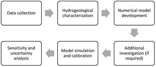
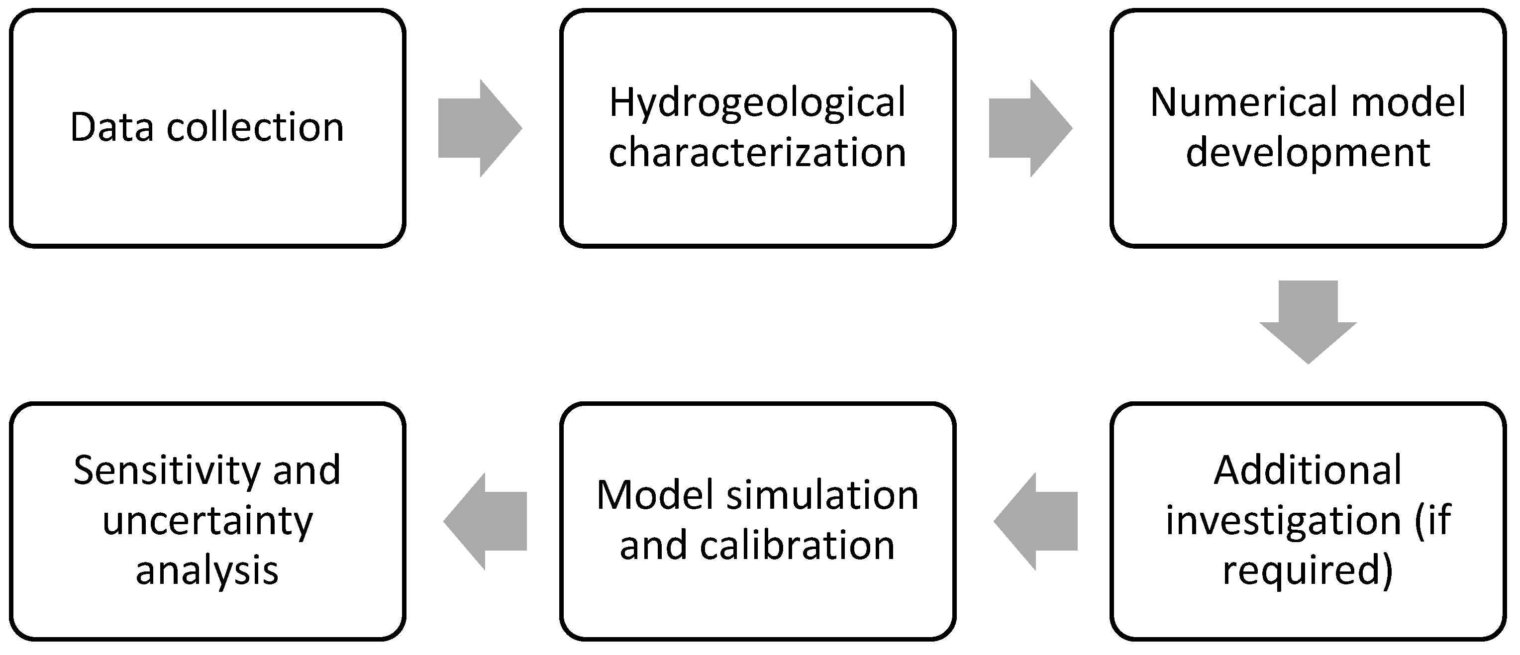
The overall methodological framework is summarized in Figure 1, which presents the sequence of stages followed in this study.

Figure 1. Methodological framework.

2.1. Data Collection

Multiple datasets were compiled to characterize the physical conditions of the study area to support the development of the numerical groundwater model. These datasets include topographic information, groundwater level measurements, tidal records, geotechnical studies, and hydraulic field testing.

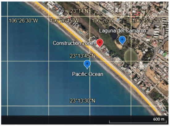
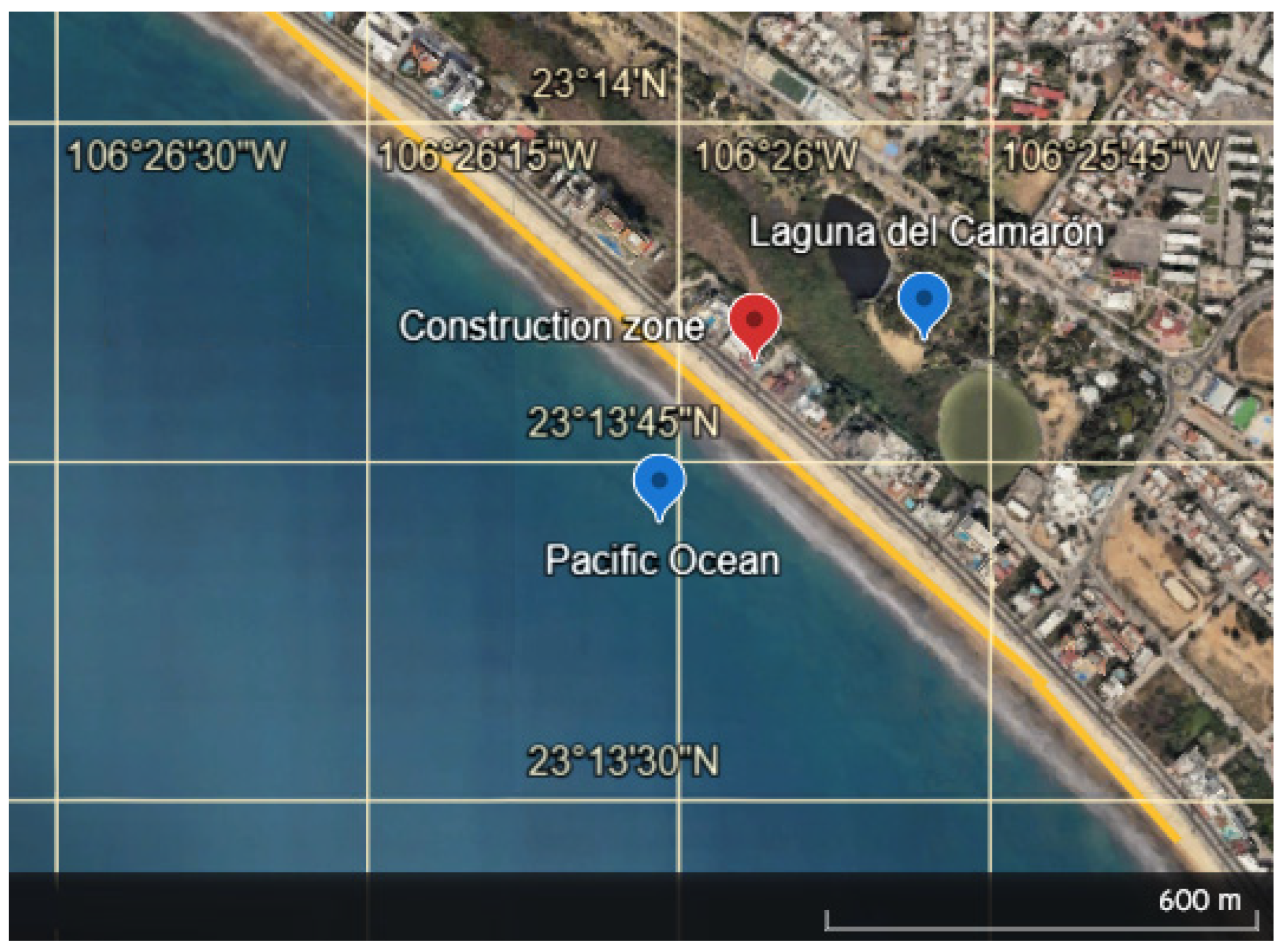
The spatial context of the study area and the main boundaries affecting groundwater dynamics are shown in Figure 2. The figure illustrates the location of the project site within the coastal urban sector of Mazatlán, including its proximity to the Pacific Ocean and the Laguna del Camarón. The Mazatlán seawall, which acts as a structural barrier is also indicated as a yellow line. Additionally, the figure highlights the position of the construction zone where the planned excavation will take place, providing a spatial reference for the hydraulic boundaries considered in the numerical model.

Figure 2. Location of the study area.

Topographic data [46] was obtained from the Instituto Nacional de Estadística y Geografía (INEGI) and processed using QGIS to generate the digital elevation model of the study area with a spatial resolution of 5 m. This information was used to define surface elevations and establish the spatial domain of the numerical model.

According to [47], this manual describes the importance of keeping piezometric record of wells, the techniques available to perform the measurement with different equipment. In this case, groundwater level measurements were collected from an observation well located within the project site. Manual measurements were performed using a Solinst Model 101 P7 water level meter. Monitoring was conducted between November 2023 and April 2024, with measurements recorded three times per day at 09:00, 12:00, and 15:00 h from Monday to Saturday.

Sea level data were obtained from the tide gauge station MZTN0402, operated by the Servicio Mareográfico Nacional [48]. These records were used to characterize tidal variability during the monitoring period and to define the hydraulic boundary condition associated with the marine influence in the numerical model.

Additionally, considering the INEGI guide [49], the hydraulic head of the sea level and the Laguna del Camarón was measured using GNSS equipment using the real time kinematic (RTK) methodology in order to reference the sea and lagoon water level to the same vertical datum.

Hydraulic properties of the aquifer were estimated through a constant-rate discharge test conducted within the study area. The results of this test were used to determine representative hydraulic conductivity values for the numerical model.

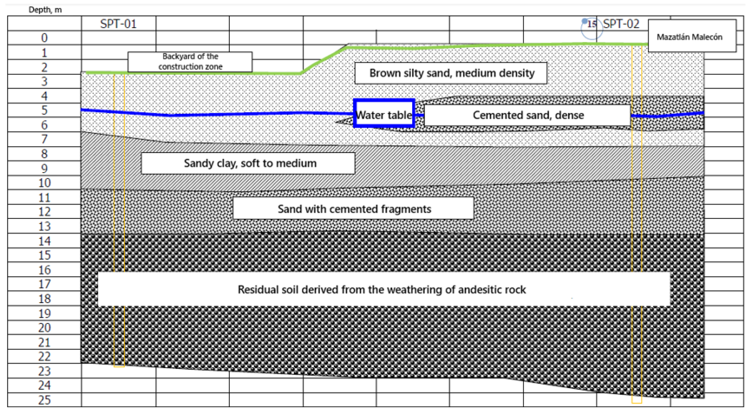
Finally, stratigraphy was obtained from a geotechnical investigation [50] carried out as part of the executive construction project. The geotechnical report provided information on soil types distribution within the study area, supporting the hydrogeological conceptualization of the aquifer system.

2.2. Hydrogeological Characterization

The hydrogeological characterization of the study area was carried out by integrating regional hydrogeological information, geotechnical investigations, and field hydraulic testing in order to define the main physical properties of the aquifer system.

According to the technical report published by CONAGUA [51], the study area is located within the Rio Presidio aquifer system, which extends across the coastal plain of Mazatlán. This aquifer is mainly composed of Quaternary alluvial and coastal deposits.

Although regional hydrogeological studies provide a general understanding of groundwater conditions within the Rio Presidio aquifer, coastal urban environments often exhibit significant local variability due to the interaction between tidal forcing, surface water bodies, and anthropogenic infrastructure. Therefore, a site-specific hydrogeological characterization was required to evaluate groundwater dynamics in the study area.

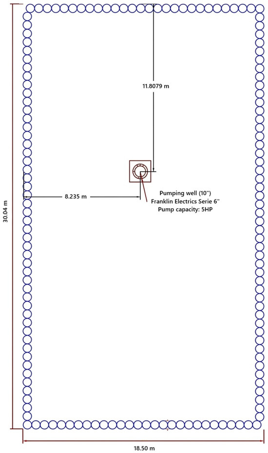
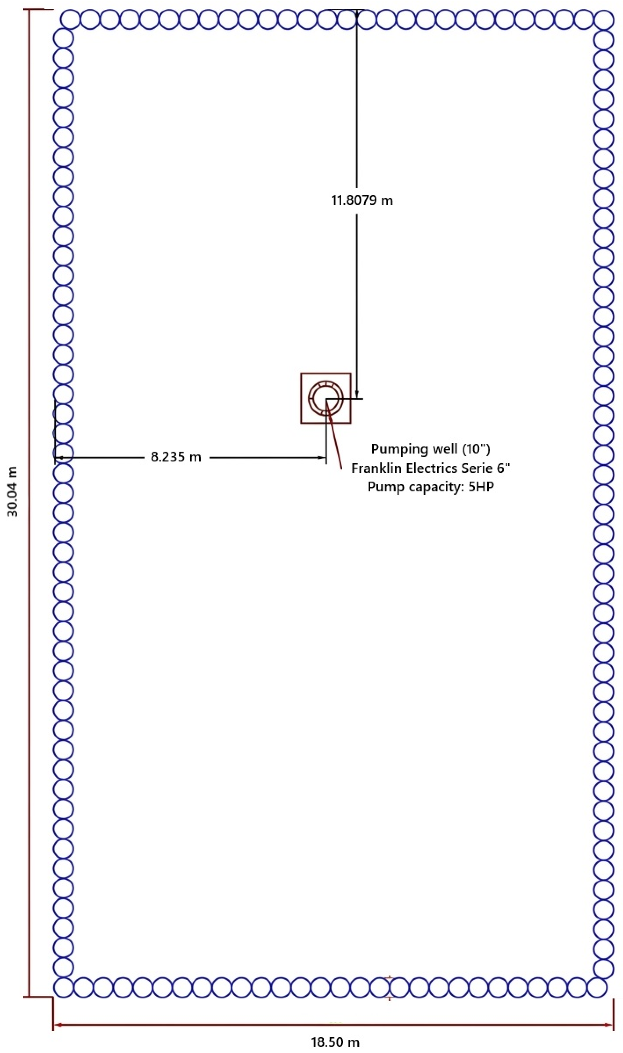
Hydraulic properties of the study area were estimated through a constant-rate pumping test. The test was performed in a 10-inch diameter well with a total depth of 8 m, using a submersible pump operating at a constant discharge rate of 10 lps. Pumping was maintained for a period of 25 min, allowing the observation of aquifer response to the induced hydraulic disturbance. Groundwater levels during pumping were monitored using the Solinst Model 101 P7 water level meter, while recovery of the water level after pumping was also recorded. The location of the pumping well within the project site is presented in Figure 3.

Figure 3. Location of the pumping well in the construction zone.

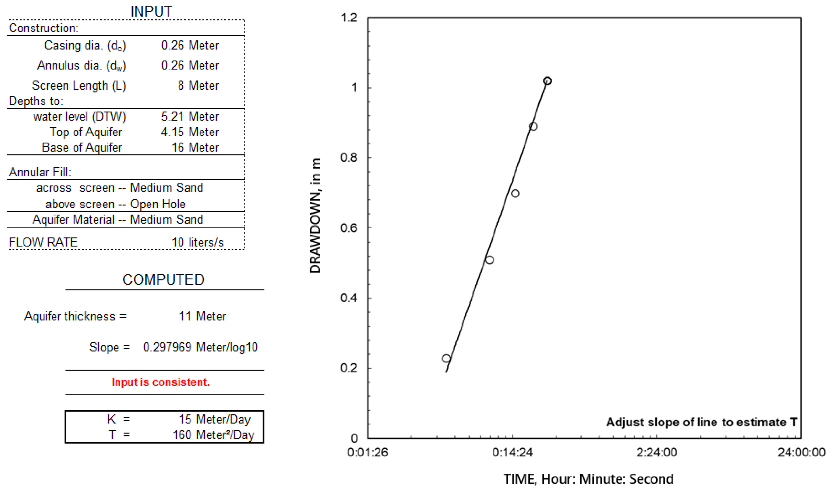
The interpretation of drawdown data was carried out using the Cooper-Jacob approximation method [52,53]. Transmissivity T was calculated as:

$$T={\displaystyle \frac{2.3\mathrm{Q}}{4\mathsf{\pi }∆\mathrm{s}}},$$

(1)

where

T = transmissivity (m²/day),

Q = pumping rate (m³/day),

∆s = change in drawdown (m).

Hydraulic conductivity K was subsequently estimated from transmissivity using the relationship:

$$K={\displaystyle \frac{T}{\mathrm{b}}},$$

(2)

where

K = hydraulic conductivity (m/day),

T = transmissivity (m²/day),

b = saturated thickness of the aquifer (m).

The hydraulic parameters from the pumping test were compared with the ranges reported in the CONAGUA report to confirm consistency with the materials identified in the study area.

Finally, climatological data were reviewed using data from operating climatological stations provided by CONAGUA near the study area [54]. Since none were available, information from private climatological stations with free access to information on the MeteoStat platform was considered [55]. Climatic conditions during the monitoring period corresponded to the dry season, with no significant precipitation events recorded. Consequently, groundwater recharge from rainfall was considered negligible based on typical runoff coefficients for urban environments [56], allowing the numerical model to focus on the hydraulic influence of tidal fluctuations, lagoon interaction and urban hydraulic boundaries.

2.3. Numerical Model Development

Groundwater dynamics were simulated using a transient numerical model developed with MODFLOW 6 [44], implemented through the graphical interface ModelMuse [45], both developed by the United States Geological Survey (USGS). The numerical code solves the three-dimensional groundwater flow equation using a finite-difference approach derived from Darcy’s law and the principle of mass conservation. The model was developed to evaluate the variability of groundwater levels under the influence of tidal fluctuations, the lagoon interaction, and a structural element present in the coastal urban system.

Groundwater flow in the aquifer system is governed by the three-dimensional transient groundwater flow equation:

$${\displaystyle \frac{\partial }{\partial x}}\left(Kx{\displaystyle \frac{\partial h}{\partial x}}\right)+{\displaystyle \frac{\partial }{\partial y}}\left(Ky{\displaystyle \frac{\partial h}{\partial y}}\right)+{\displaystyle \frac{\partial }{\partial z}}\left(Kz{\displaystyle \frac{\partial h}{\partial z}}\right)+\mathrm{W}=\mathrm{S}\mathrm{s}{\displaystyle \frac{\partial h}{\partial t}},$$

(3)

where

Kx, Ky, Kz = hydraulic conductivity in the x, y and z directions (m/day),

h = hydraulic head (m),

W = volumetric flux per unit volume (1/day),

Ss = specific storage (1/m),

t = time (day).

This equation describes groundwater flow under transient conditions, allowing the simulation of hydraulic head variations caused by time-dependent boundary conditions. It is important to note that the Complementary Technical Standards for Construction and Design of Foundations [57] specify that the analysis of groundwater flow must be carried out under the transient state condition.

According to [58], the conceptual model considers the hydraulic interaction between groundwater and the main boundaries in the system, including the Pacific Ocean, the Laguna del Camarón, and the Mazatlán seawall, which acts as a barrier modifying natural groundwater flow patterns.

The model domain was defined with dimensions of 1.39 km in length and 0.74 km in width. The spatial discretization was implemented using a finite-difference grid generated in ModelMuse. Considering the spatial resolution of available topographic data, this value was obtained from the INEGI digital elevation model with a resolution of 5 m.

The aquifer system was represented by a single model layer, consistent with hydrogeological conditions identified in the study area. The top elevation of the model layer was derived from the processed digital elevation model.

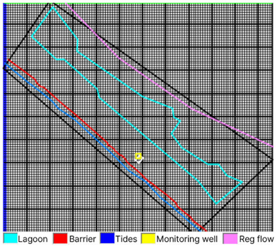
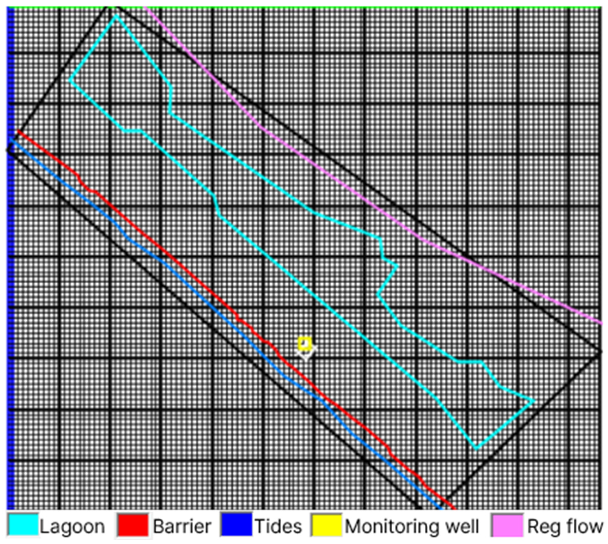
Hydraulic boundary conditions were defined to represent the principal external controls governing groundwater flow in the system. The spatial configuration of the model is illustrated in Figure 4. The figure shows the extent of the computational domain, the grid and the relative position of the main boundaries influencing the system.

Figure 4. Numerical model grid within main boundaries.

The hydraulic influence of the Pacific Ocean (tides) was represented using the General Head Boundary (GHB) package in MODFLOW 6.

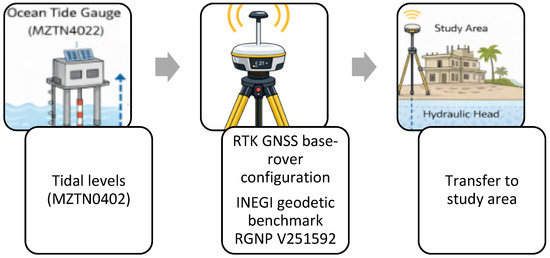
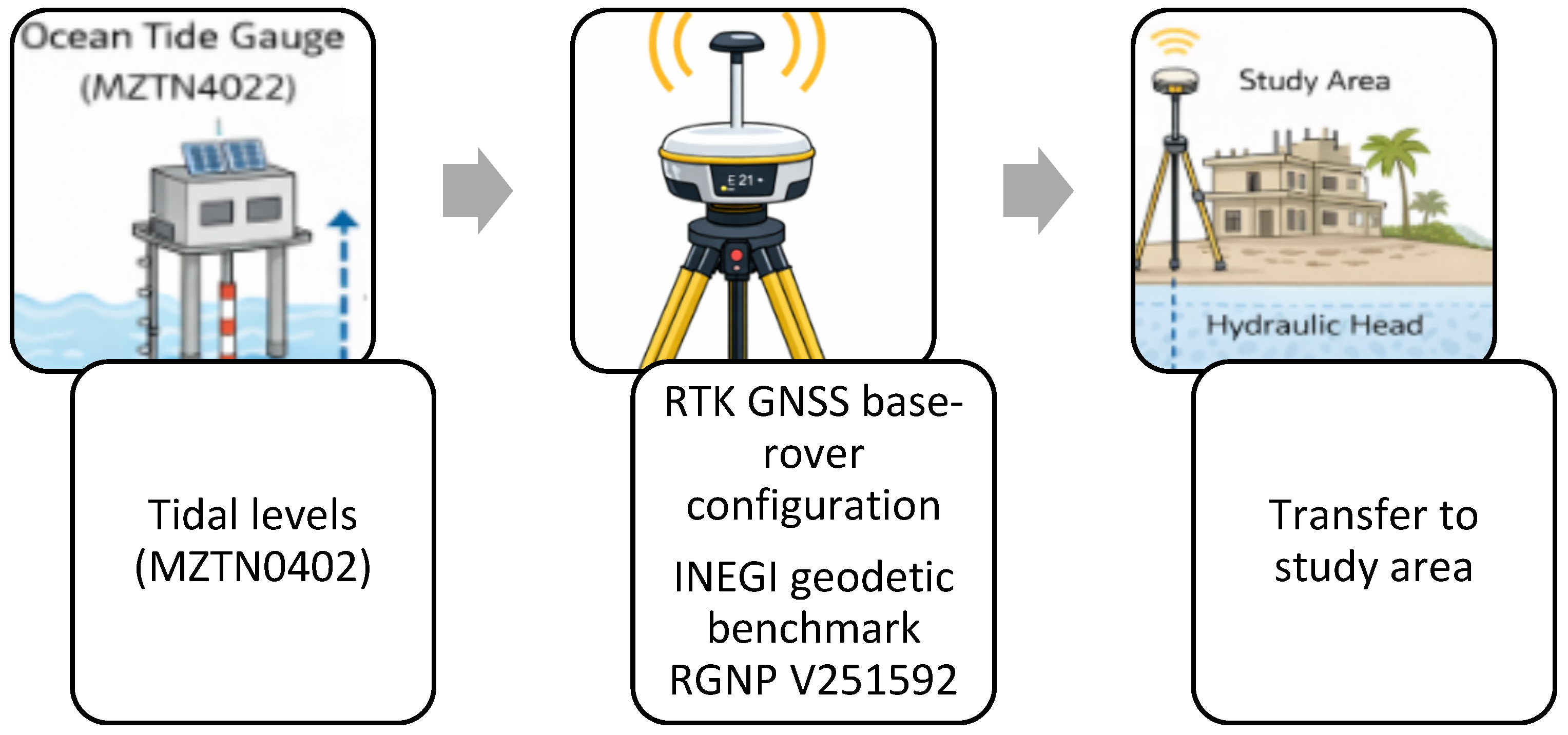
Time-dependent hydraulic heads used for this boundary were derived from tidal records obtained at the Mazatlán tide gauge station (MZTN0402). To ensure consistency between the vertical datum of the tide gauge and the project site, RTK GNSS surveying techniques were used to transfer elevation references [49]. The survey was conducted using a dual-frequency differential GNSS system (SingularXYZ, model E1) operating in a base-rover configuration, with the official INEGI geodetic benchmark RGNP V251592 serving as the reference point. The procedure used to transfer the vertical reference and determine the hydraulic head at the study site is illustrated in Figure 5.

Figure 5. Transfer of tidal elevation reference to the study area.

After transferring the vertical reference from the tide gauge station to the study area, the tidal elevations were adjusted to the local vertical datum used in the numerical model. The hydraulic head applied to GHB was analyzed by adding the elevation correction between the tide gauge reference and the study area datum. This correction can be expressed as:

$$H_{GHB}\left(t\right)=H_{tide}\left(t\right)+ ∆z,$$

(4)

where

H_GHB (t) = Hydraulic head applied to GHB at time t (masl),

H_tide (t) = Tidal elevation recorded at the MZTN0402 tide station (m),

∆z = vertical correction used to transfer the tidal datum to the study area (m).

The hydraulic interaction between groundwater and the Laguna del Camarón (lagoon) was represented using the LAK package, which simulates groundwater–surface water exchange through a conductance-controlled flux. Lagoon water levels were defined based on discrete observations from GNSS-RTK measurements, corresponding to specific time intervals, and were assumed to remain constant throughout each day. These values were implemented using stress periods, where each assigned water level remains constant within the corresponding time step simulated. Transitions between different water levels occur at the boundaries of consecutive stress periods, resulting in a discretized temporal representation of water level variations.

Additionally, the Mazatlán seawall (barrier) was incorporated using the Horizontal Flow Barrier (HFB) package, which reduces hydraulic connectivity between adjacent model cells along the barrier alignment.

Beyond the local boundary conditions associated with tidal and lagoon interaction, a regional flow condition was incorporated with a GHB package to represent the natural hydraulic gradient of the aquifer.

To evaluate groundwater level variations, an observation point (monitoring well) was defined using the Observation (OBS) utility available in MODFLOW 6. The observation point represents the well located outside the immediate construction area, where groundwater levels were periodically measured. The simulated groundwater levels obtained at this monitoring well were subsequently compared with field measurements. This comparison allowed the evaluation of model performance and served as the basis for the calibration procedure described in the following section.

The numerical simulations were performed under transient conditions, allowing groundwater levels to respond dynamically to time-varying boundary conditions. This approach enables the evaluation of groundwater level under conditions relevant to construction planning.

2.4. Additional Investigation (If Required)

Additional investigation was conducted to identify potential factors influencing the observed dynamic in groundwater levels. This analysis aimed to determine whether the maximum piezometric levels observed each month were associated with specific external forces.

The investigation focused on evaluating the relationship between groundwater level fluctuations and boundary-condition variations in the hydrogeological system. Three main variables were considered: (1) precipitation events, (2) astronomical tides, and (3) hydraulic interaction with the lagoon.

Precipitation data were obtained from the meteorological station 76,459 (nearest station), available through the Meteostat climate data platform [55]. Meteostat is an open access meteorological database that presents weather observations, providing quality-controlled information. The selected station provides representative information, allowing the identification of precipitation events during the evaluation period between November 2023 and April 2024.

Tidal records obtained from the Mazatlán tide gauge station were analyzed to identify periods associated with astronomical tidal conditions. To further evaluate whether groundwater levels could be related to specific lunar phases, the lunar phase records for Mazatlán were reviewed using the database available at the platform time and date [59,60]. This platform provides detailed astronomical information, including lunar phases and their timing for specific geographic locations.

The timing of maximum monthly groundwater levels recorded at the observation well was compared with these variables to evaluate and provide contextual information for selecting representative monitoring periods used later in the model simulation and calibration process.

Finally, the information required to feed the HFB package was obtained from an engineer who was present during a modification process of the seawall in 2019, confirming that for the study area the height of the seawall was 5 m.

2.5. Model Simulation and Calibration

The numerical model was simulated under transient conditions to reproduce groundwater level variations during the monitoring period. The transient simulation allowed the representation of time-dependent hydraulic responses.

Groundwater level observations were obtained from a monitoring well outside the immediate construction zone. Measurements were collected three times per day (09:00, 12:00, and 15:00) during selected days corresponding to where maximum levels were observed monthly.

Simulated groundwater levels used for calibration were extracted using the OBS package implemented in MODFLOW 6.

Model calibration consisted of comparing simulated groundwater levels with observed measurements. Model performance was evaluated using statistical indicators that quantify the agreement between simulated and observed values [24].

The root mean square error (RMSE) was calculated as (5) and the mean absolute error (MAE) was calculated as (6):

$$RMSE=\sqrt{{\displaystyle \frac{1}{n}}{\displaystyle {\sum }_{i=1}^n}{(hobs-hsim)}^2},$$

(5)

$$MAE={\displaystyle \frac{1}{n}}{\displaystyle {\sum }_{i=1}^n}{(hobs-hsim)}^2,$$

(6)

where

hobs = observed groundwater level (m),

hsim = simulated groundwater level (m),

n = total number of observations.

These statistical indicators were used to assess the ability of the numerical model to reproduce groundwater level variations [61,62].

2.6. Sensitivity and Uncertainty Analysis

A sensitivity and uncertainty analysis were conducted to identify the parameters that most strongly affect the response of the numerical model [62,63]. The sensitivity analysis was performed using a One-at-a-Time (OAT) approach. The parameters selected for the analysis were: tidal boundary condition, hydraulic interaction with the Laguna del Camarón, and hydraulic conductivity.

For each parameter (p), a reference value (p₀) corresponding to the calibrated model was defined. As mentioned in [64], a relative perturbation of ±20% was applied to generate two additional parameter values:

$$p^{+}=p_0(1+0.20),$$

(7)

$$p^{-}=p_0\left(1-0.20\right).$$

(8)

To further support the selected perturbation magnitude, its physical implications were evaluated for key boundary conditions, particularly those associated with tidal forcing and lagoon interaction.

Each perturbed parameter produced an independent model simulation, ensuring that the resulting variation in groundwater levels could be attributed to the modified parameter.

The response variable used to quantify model sensitivity was the maximum simulated hydraulic head at the observation well. This variable was defined as:

$$y=h_{max},$$

(9)

where

y = response variable (m),

h_max = maximum simulated groundwater level (m).

The influence of each parameter on the system response was evaluated through the absolute change in the response variable:

$${∆y}^{+}=y\left(p^{+}\right)-y\left(p_0\right),$$

(10)

$${∆y}^{-}=y\left(p^{-}\right)-y\left(p_0\right).$$

(11)

This procedure allows us to identify the parameters that dominate the hydrogeological system.

Following the sensitivity analysis, a deterministic uncertainty propagation analysis was conducted. For each parameter p_i, an uncertainty interval was defined around the calibrated value p_i,0:

$$p_i\in \left[p_{i,0}\left(1-\delta \right), p_{i,0}\left(1+\delta \right)\right] ,$$

(12)

where

p_i,0 = calibrated parameter value,

δ = relative uncertainty (±20).

Assuming independence among parameters, the combined uncertainty of the simulated groundwater level was estimated through the quadratic propagation of individual effects:

$${\sigma }_y =\sqrt{{(∆y_{tide})}^2+{(∆y_{lagoon})}^2+{(∆y_K)}^2},$$

(13)

where

∆y_tide = groundwater level variation induced by tidal boundary (m),

∆y_lagoon = variation associated with lagoon interaction (m),

∆y_K = variation associated with hydraulic conductivity (m).

This methodology provides a quantitative estimation of the uncertainty range associated with the simulated groundwater levels and allows the identification of the dominant factors controlling the hydrogeological response of the system.

3. Results

3.1. Identification of Critical Piezometric Conditions

Groundwater level monitoring was conducted between November 2023 and April 2024. Measurements were taken three times per day, generating a dataset that allowed the identification of the days with the highest monthly piezometric levels.

These days were selected as representative critical conditions for the system, since they correspond to periods when the groundwater level approaches its maximum elevation; this condition is relevant for construction activities involving excavations below the groundwater table.

Table 1 summarizes the 18 piezometric observations (the day with the highest piezometric level observed monthly during the monitoring period).

Table 1. Selected day of the month where highest groundwater level was recorded.

Date	Time	Observed Groundwater Level (masl)
14 November 2023	09:00	0.24
	12:00	0.36
	15:00	0.53
13 December 2023	09:00	0.17
	12:00	0.29
	15:00	0.46
11 January 2024	09:00	0.14
	12:00	0.26
	15:00	0.44
9 February 2024	09:00	0.11
	12:00	0.25
	15:00	0.38
9 March 2024	09:00	−0.06
	12:00	0.14
	15:00	0.35
9 April 2024	09:00	−0.10
	12:00	0.01
	15:00	0.31

The observed groundwater levels ranged between −0.10 to 0.53 masl, indicating significant fluctuations in the system.

3.2. Hydrological Conditions During the Monitoring Period

To understand the factors controlling groundwater dynamics, the hydrological conditions during the monitoring period were analyzed considering three potential factors:

• precipitation;
• tidal forcing;
• lagoon interaction.

Meteorological data obtained from the Meteostat platform were analyzed to evaluate whether precipitation could have contributed to groundwater recharge during the monitoring period. For this purpose, the day with the highest piezometric level recorded each month (Table 1) was evaluated together with a 48 h observation window to determine if rainfall events occurred prior to the groundwater measurements that could have influenced the system.

The analysis indicated that no significant precipitation events occurred during the evaluated period that could represent a relevant recharge factor. Only one rainfall event was identified on 12 November 2023, with a cumulative precipitation of 18.2 mm recorded two days before the selected critical day.

To estimate the potential contribution of this event to groundwater recharge, a runoff coefficient was considered. According to [56], typical runoff coefficients in urban environments range between 0.7 and 0.95, which implies that only 5–30% of the total precipitation may infiltrate. Based on this range, the effective infiltration associated with the recorded event would be between 0.91 and 5.46 mm, with an average value of 3.18 mm. This level of recharge is relatively small when compared to the observed groundwater fluctuations during the monitoring period, which ranged from −0.10 to 0.53 masl. In addition, groundwater levels influenced by tidal forcing ranged between −0.407 to 1.527 masl, indicating that tidal dynamics contribute significantly more to groundwater level variations than precipitation. Furthermore, the study area is predominantly impermeabilized due to concrete and the presence of drainage infrastructure, which reduces infiltration capacity.

Another precipitation event of 12.6 mm was recorded on 15 February, but rainfall occurred several days after the critical piezometric day identified for February. Consequently, this event was not considered relevant to the numerical model evaluation for that month.

Overall, the monitoring period corresponded to the regional dry season, indicating that precipitation did not play a significant role in groundwater fluctuations. These results support the interpretations that tidal forcing may represent the primary factor of groundwater variations in the study area.

In contrast, the analysis of tidal records from the Mazatlán tide gauge station (MZTN0402) revealed a strong correspondence between the days with maximum piezometric levels and periods of astronomical tides associated with the new moon phase.

The lunar phases were verified using the timeanddate platform, which confirmed that the selected critical days coincided with periods of maximum tidal amplitude. Table 2 summarizes the day and hour of maximum tidal levels recorded, together with the corresponding astronomical tidal date and hour.

Table 2. Date and time of tidal maximum and new moon phase relationship.

Month	Date and Time of Tidal Maximum	Date and Time of New Moon Phase
November	14 November 2023–15:07	13 November 2023–02:27
December	13 December 2023–14:51	12 December 2023–16:31
January	11 January 2024–15:01	11 January 2024–04:57
February	9 February 2024–15:07	9 February 2024–15:59
March	9 March 2024–14:45	10 March 2024–02:00
April	9 April 2024–03:11	8 April 2024–11:20

The results indicate that the maximum tidal levels consistently occurred during periods associated with the new moon phase. This correspondence suggests that groundwater levels observed are strongly influenced by astronomical tides (new moon phase) in the study area.

3.3. Input Data and Numerical Model Configuration

Once the critical hydrological conditions were identified, the 18 observed piezometric measurements were used as reference data for the numerical model calibration.

The model was parameterized using hydrogeological information obtained from multiple sources (see Appendix A), including:

• In situ pumping tests used to estimate hydraulic conductivity (Appendix A.1),
• Geotechnical soil exploration (Appendix A.2),
• Regional hydrogeological information from the Rio Presidio aquifer report,
• Tidal records obtained from the Mazatlán tide gauge station MZTN0402 (Appendix A.3),
• Hydraulic head measurements associated with the Laguna del Camarón.

The hydraulic conductivity of the aquifer was estimated from the pumping test. The analysis of the drawdown data using the Cooper–Jacob approximation yielded a hydraulic conductivity value of 15 m/day and a transmissivity of 160 m²/day, values consistent with the sandy materials identified in the geotechnical investigation. The technical report of Río Presidio aquifer from CONAGUA provides regional estimates of hydraulic properties and groundwater conditions that were used as reference values during the model parameterization.

The numerical model was discretized using a structured grid with horizontal cell dimensions of 10 m × 10 m in 139 columns and 74 rows. The model was represented using a single-layer configuration, consistent with aquifer conditions observed at the site.

The principal boundary conditions incorporated in the model include: (1) tidal influence from the Pacific Ocean, represented with the GHB package, (2) interaction with the Laguna del Camarón, represented with LAK package, and (3) the Malecón seawall, represented with the HFB package.

The vertical transfer indicated that the reference elevation at the study site differs from the tide gauge datum by ∆z = 1.735 m. Consequently, tidal elevations recorded were corrected before in the numerical model. It is important to mention that groundwater level measurements were taken three times per day at 09:00, 12:00, and 15:00 h. Because tidal data obtained from the MZTN0402 tide gauge station are recorded at one-minute intervals, the tidal elevations were temporally matched with the corresponding piezometric observation times and the hydraulic head associated with the Laguna del Camarón. Table 3 presents the paired dataset used in the analysis.

Table 3. Observed piezometric levels and time-dependent hydraulic head values (GHB and LAK).

Day	Hour	Piezometric Observed Level (masl)	Tidal Elevation in the Study Area (masl)	Hydraulic Head Associated with the Lagoon (m)
14 November 2023	09:00	0.24	0.436	0.77
	12:00	0.36	0.937
	15:00	0.53	1.527
13 December 2023	09:00	0.17	0.475	0.82
	12:00	0.29	0.979
	15:00	0.46	1.481
11 January 2024	09:00	0.14	0.395	0.73
	12:00	0.26	0.911
	15:00	0.44	1.451
9 February 2024	09:00	0.11	0.242	0.64
	12:00	0.25	0.832
	15:00	0.38	1.474
9 March 2024	09:00	−0.06	−0.035	0.68
	12:00	0.14	0.696
	15:00	0.35	1.359
9 April 2024	09:00	−0.10	−0.407	0.71
	12:00	0.01	0.001
	15:00	0.31	0.944

Finally, Table 4 summarizes the principal input parameters used in the numerical configuration.

Table 4. Parameters input for the numerical model configuration.

Parameter	Value	Units	Source
Hydraulic conductivity (K)	15	m/day	Pumping test
Transmissivity (T)	160	m2/day	Pumping test
Model cell size	10 × 10	M	Model discretization
Model domain	1.39 × 0.74	Km	Study area
Aquifer type	Unconfined	-	Technical report
Stratigraphy	Medium sand	-	Geotechnical investigation

The transient simulations were performed to the selected critical days identified in Section 3.1.

3.4. Numerical Simulation

The numerical results indicate that the aquifer responds dynamically to tidal fluctuations, producing short-term groundwater level variations. The simulated groundwater levels show a clear temporal response to the variations in the tidal boundary condition, confirming that tidal forcing is the dominant mechanism controlling the short-term groundwater dynamics of the study zone.

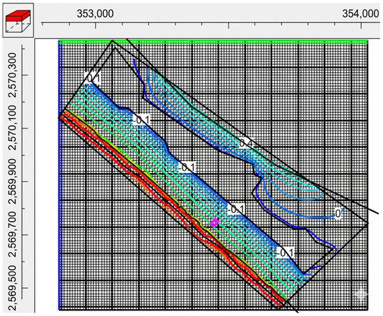
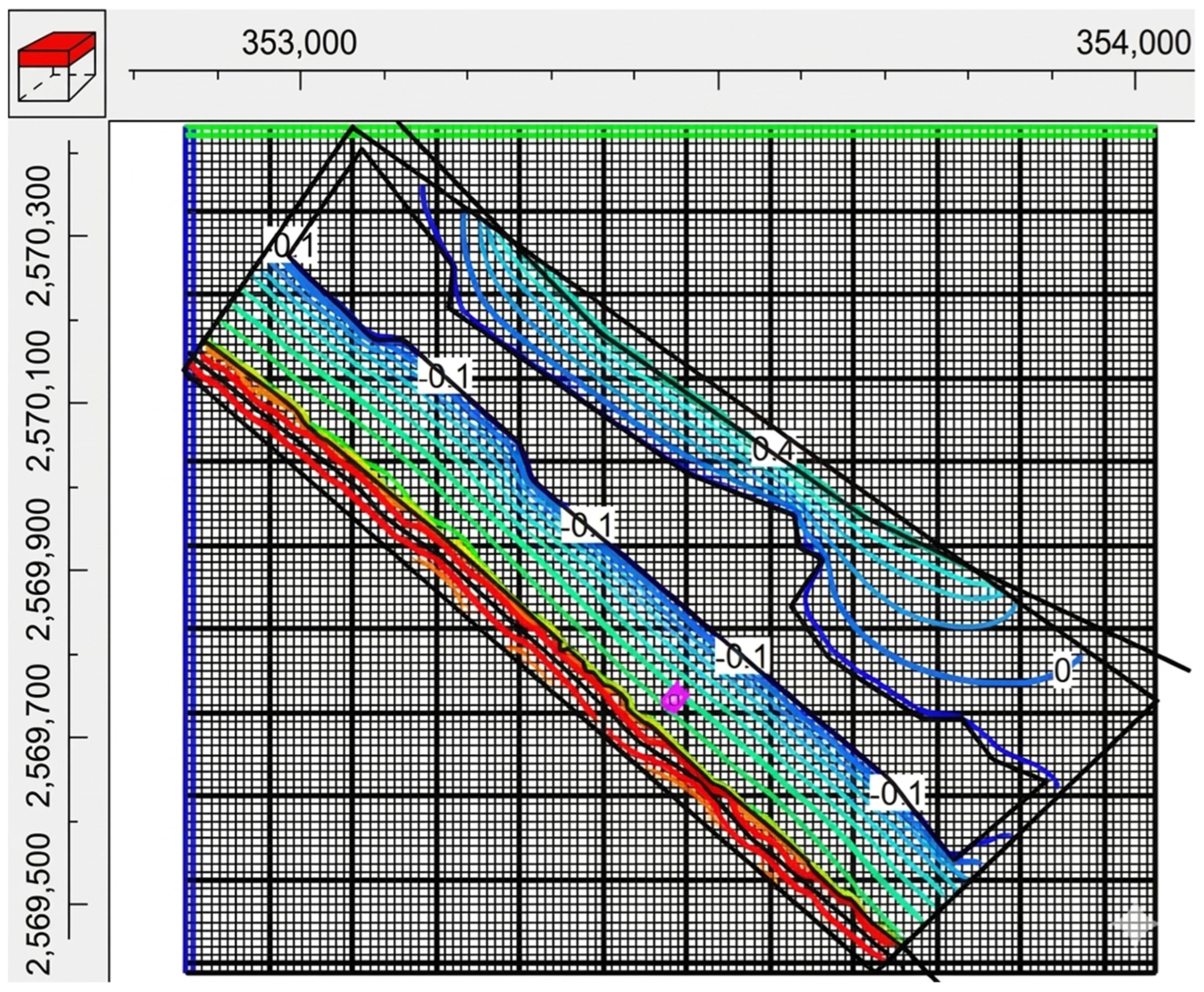
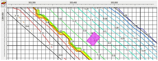
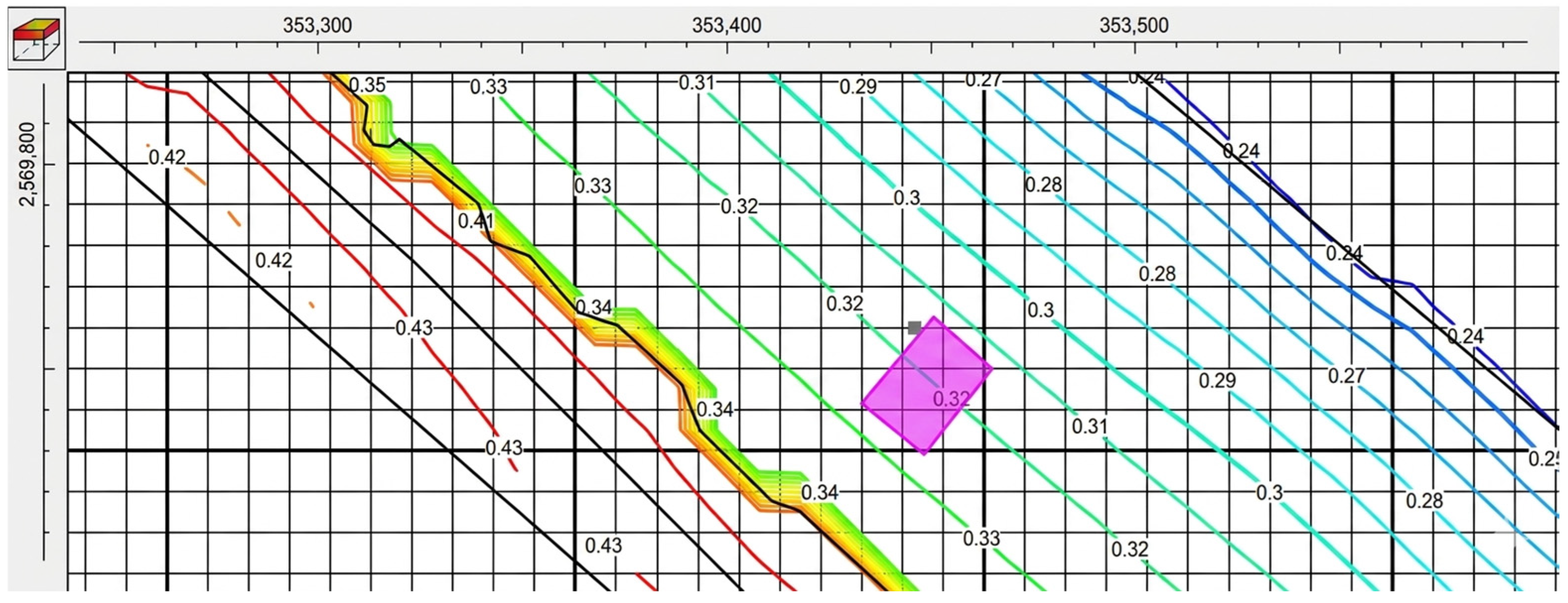
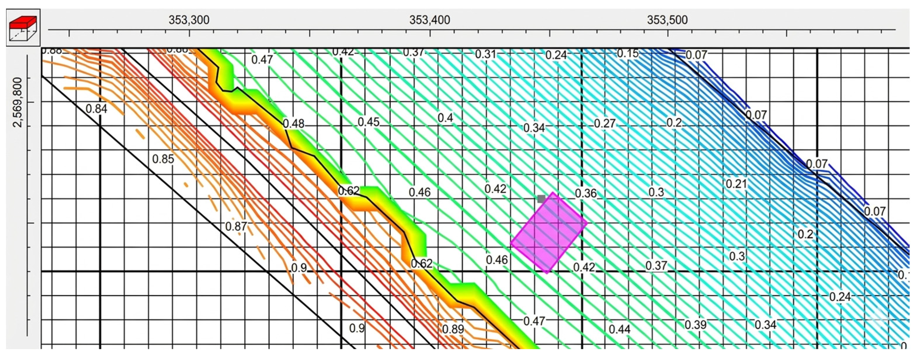
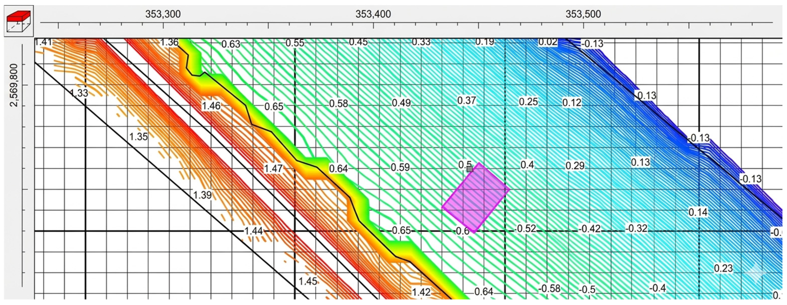
The contour maps presented in Figure 6, Figure 7, Figure 8 and Figure 9 correspond to isolines of hydraulic head (equipotential lines), displayed using a rainbow color scheme to represent the spatial distribution of groundwater levels (in masl) across the model domain. Each contour line connects points of equal hydraulic head, allowing visualization of the groundwater flow field.

Figure 6. Numerical model result for November (the entire domain).

Figure 7. Numerical model result for November (09:00).

Figure 8. Numerical model result for November (12:00).

Figure 9. Numerical model result for November (15:00).

Figure 6 shows the complete numerical model domain, including its spatial discretization and the general simulated hydraulic head distribution for the critical scenario of 14 November 2023. The model domain has approximate dimensions of 1390 m × 740 m, with a uniform grid discretization of 10 × 10 m, as described in Table 4. In Figure 6, the area of interest for the planned construction process is identified by a solid pink polygon. This highlighted zone corresponds to the region analyzed in subsequent figures.

Figure 7, Figure 8 and Figure 9 present detailed views of the highlighted zone, focusing on the local groundwater response under transient conditions at 9:00, 12:00 and 15:00 h, respectively. These figures illustrate the temporal variation of groundwater levels in the vicinity of the construction site. Additionally, a gray point located adjacent to the pink polygon represents the observation well used during the calibration process to compare simulated and observed groundwater levels.

Although the spatial distribution of the hydraulic head is illustrated for the November scenario, numerical simulations were performed for all the selected monitoring days and time steps. To facilitate comparison between observed and simulated groundwater levels, the results for the 18 conditions (six days and three-time steps per day) are summarized in Table 5.

Table 5. Observed piezometric levels and simulated levels.

Day	Hour	Observed Hydraulic Head (masl)	Simulated Hydraulic Head (masl)
14 November 2023	09:00	0.24	0.315866
	12:00	0.36	0.398107
	15:00	0.53	0.501742
13 December 2023	09:00	0.17	0.230834
	12:00	0.29	0.348725
	15:00	0.46	0.477942
11 January 2024	09:00	0.14	0.196723
	12:00	0.26	0.320904
	15:00	0.44	0.468210
9 February 2024	09:00	0.11	0.061378
	12:00	0.25	0.205320
	15:00	0.38	0.381399
9 March 2024	09:00	−0.06	0.018105
	12:00	0.14	0.182957
	15:00	0.35	0.350492
9 April 2024	09:00	−0.10	−0.06316
	12:00	0.01	−0.082544
	15:00	0.31	0.219072

The comparison between observed and simulated groundwater levels indicates that numerical model reproduces the temporal response of the water table to tidal forcing.

3.5. Numerical Calibration

The calibration of the numerical model was carried out by comparing the observations recorded for the monthly maximum piezometric conditions with the simulated groundwater levels.

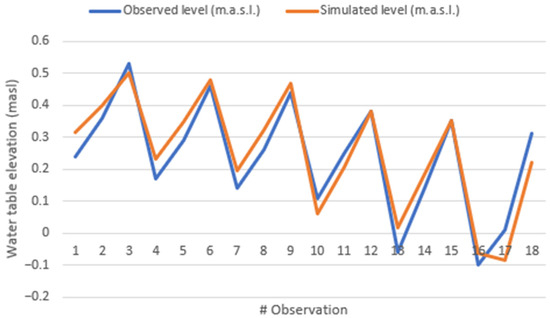
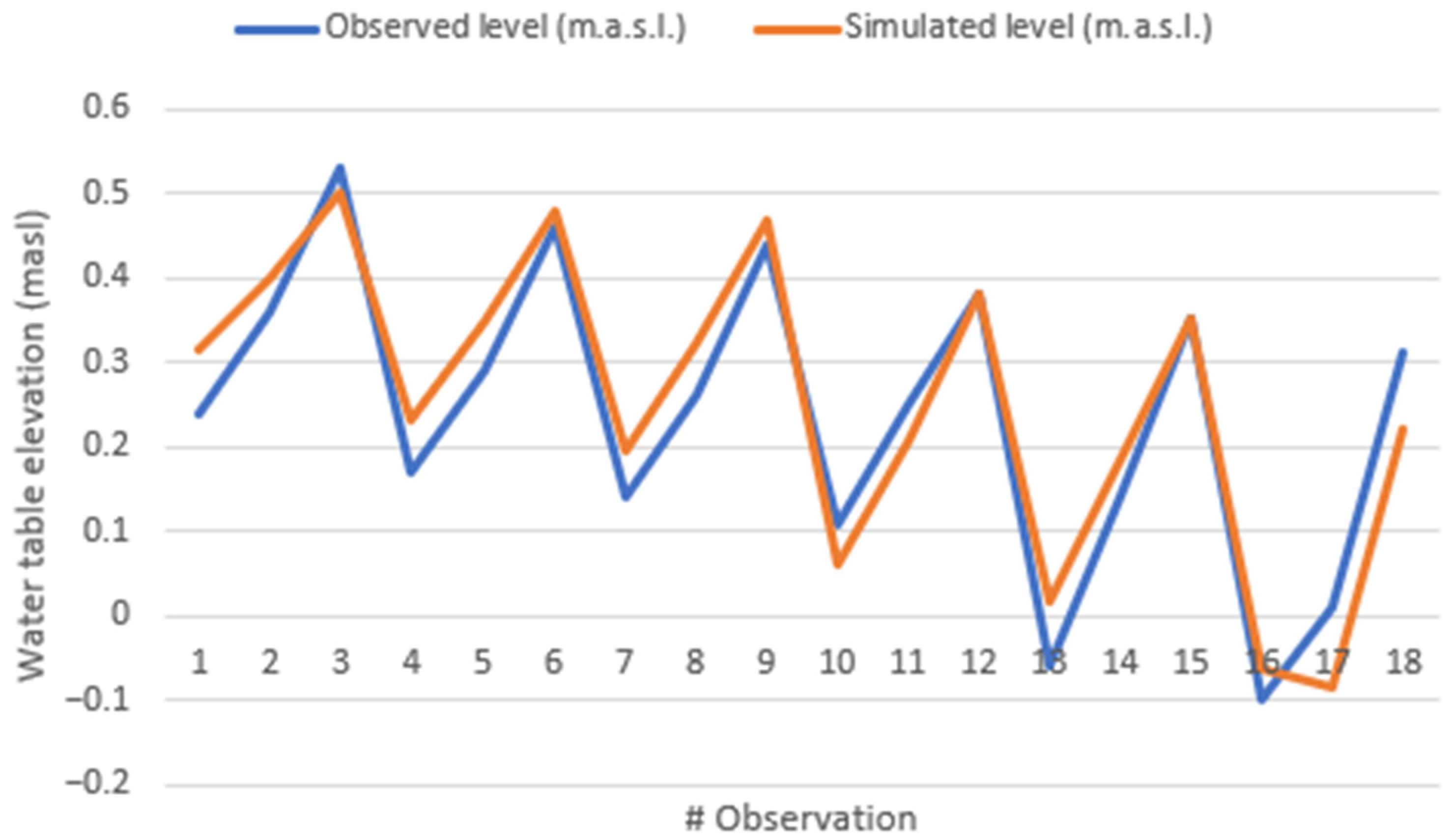
Model performance was evaluated using the RMSE, and the MAE, which quantify the difference between observed and simulated groundwater levels. Considering the 18 observations, the numerical model produced an RMSE of 0.056 m and an MAE of 0.049 m, indicating a strong agreement between simulated and observed groundwater levels. Table 6 summarizes the residual differences between both datasets, while Figure 10 illustrates the comparison between simulated and observed groundwater levels for the evaluated conditions.

Table 6. Observed and simulated level comparison (Residual).

Day	Hour	# Observation	Observed Level (masl)	Simulated Level (masl)	Residual (masl)
14 November 2023	09:00	1	0.24	0.315866	−0.075866
	12:00	2	0.36	0.398107	−0.038107
	15:00	3	0.53	0.501742	0.028258
13 December 2023	09:00	4	0.17	0.230834	−0.060834
	12:00	5	0.29	0.348725	−0.058725
	15:00	6	0.46	0.477942	−0.017942
11 January 2024	09:00	7	0.14	0.196723	−0.056723
	12:00	8	0.26	0.320904	−0.060907
	15:00	9	0.44	0.468210	−0.028210
9 February 2024	09:00	10	0.11	0.061378	0.048622
	12:00	11	0.25	0.205320	0.044680
	15:00	12	0.38	0.381399	−0.001399
9 March 2024	09:00	13	−0.06	0.018105	−0.078105
	12:00	14	0.14	0.182957	−0.042957
	15:00	15	0.35	0.350492	−0.000492
9 April 2024	09:00	16	−0.10	−0.06316	−0.036840
	12:00	17	0.01	−0.082544	0.092544
	15:00	18	0.31	0.219072	0.090928

Figure 10. Simulated and observed groundwater levels.

During the six-month evaluation period, groundwater levels ranged from −0.10 to 0.53 masl, representing fluctuations of approximately 0.63 m. This information is particularly relevant for construction planning in coastal environments where excavations may occur near or below the water table. Such variability can influence excavation stability, the performance of dewatering systems, and the selection of construction methods. Therefore, understanding the temporal variability of groundwater levels is essential for anticipating critical conditions and optimizing construction practices.

3.6. Sensitivity and Uncertainty Results

The analysis was conducted using the OAT method, in which a single parameter is varied while the remaining parameters are kept constant at their calibrated values. This allows the individual influence of each parameter on the model response to be isolated and quantified.

The parameters selected for the sensitivity analysis where those considered relevant for controlling groundwater dynamics. These included: (1) Hydraulic conductivity (K), (2) tidal elevation with the GHB package, and (3) hydraulic head of the lagoon with the LAK package.

For the sensitivity analysis, each parameter was varied within a ±20% range relative to the calibrated value (considering the positive as a critical scenario for construction activities). This assumption reflects the need to evaluate the possible increase in groundwater levels that could affect excavation stability and groundwater control strategies.

The resulting changes in simulated groundwater levels indicate that the numerical model is most sensitive to tidal influence. In contrast, the model showed lower sensitivity to variations in the hydraulic conductivity. Table 7 shows the impact of the +20% parameters perturbations on simulated groundwater level.

Table 7. Sensitivity analysis (perturbation of +20%).

Parameter	Value	Value (+20%)	Groundwater Level Variation	Relative Influence (Qualitative)
Hydraulic conductivity (K)	15 m/day	18 m/day	+0.05 m	Low
Tidal elevation	1.575 masl	1.89 masl	+0.30 m	High
Hydraulic head (lagoon)	0.82 m	0.984 m	+0.17 m	Medium

The selected perturbation magnitude of +20% is justified as follows: (i) for tidal influence, considering a maximum recorded tidal elevation of 1.93 masl (up to 2024) from [48], the maximum hydraulic head observed within the study area during the analysis period was 1.575 masl. A 20% increase results in a value of 1.89 masl, which is very close to the historical maximum recorded level. This represents a realistic critical scenario that has already occurred and may occur again under extreme conditions.

Similarly, for the Laguna del Camarón, which was simulated using the LAK package, the maximum hydraulic head observed was 0.82 masl. A +20% perturbation yields a value of 0.984 masl, which is close to the maximum storage capacity of the lagoon of 1.0 masl as determined from GNSS-RTK field measurements.

This indicates that the selected perturbation magnitude generates physically meaningful scenarios that approach known critical thresholds without exceeding realistic system limits, thereby supporting its suitability for sensitivity analysis.

To evaluate model uncertainty, the range of simulated groundwater levels resulting from the parameter perturbations was analyzed. Based on the previous result, a deterministic propagation of uncertainty was performed to estimate the expected range of variation of the maximum groundwater level. This analysis quantifies the contribution of each parameter to the total uncertainty of the simulated groundwater level. The result of the total uncertainty is presented in Table 8.

Table 8. Contribution of parameters to groundwater level uncertainty.

Source of Uncertainty	Groundwater Level Variation	Total Uncertainty
Hydraulic conductivity (K)	+0.05 m
Tidal elevation	+0.30 m	+0.35 m
Hydraulic head (lagoon)	+0.17 m

Overall, the estimated total uncertainty of +0.35 m represents the expected range of variation in simulated groundwater levels under the evaluated conditions. This result highlights the importance of accurately characterizing tidal boundary conditions when modeling groundwater dynamics in coastal environments and provides a quantitative range for potential groundwater level variability, which is particularly relevant for the planning of excavation and groundwater control strategies in coastal construction projects.

4. Discussion

4.1. Interpretation of Results

The results obtained from the numerical model indicate that tidal forcing is the dominant factor controlling groundwater fluctuations of the study area. The calibration metrics obtained for the model (MAE = 0.049 m and RMSE = 0.056 m) demonstrate that the implemented numerical model framework is capable of reproducing the observed groundwater dynamics with accuracy.

It is important to emphasize that the calibration process was focused on maximum piezometric records, which represent the most critical conditions for construction purposes. Unlike generalized hydrogeological studies that aim to reproduce long-term average behavior, this approach prioritizes short-term extreme conditions that directly affect excavation stability, flooding into the excavation and groundwater control design [17,65]. The use of local data allows for an accurate representation of groundwater behavior and supports decision-making within shorter time scales relevant to construction activities.

A key finding of this study is the relationship between maximum groundwater levels and astronomical tidal conditions. The analysis of piezometric records showed that the peak groundwater levels consistently occur during periods of new moon, indicating that this phase significantly influences inland groundwater dynamics. However, it is important to note that every study area is different and the dominant lunar phase influencing groundwater levels may vary. A study [2] reported three cases in which two areas exhibited a stronger influence from full moon tides, whereas one zone was primarily driven by new moon conditions. In this study, the results clearly indicate that, during the analyzed period, new moon tidal conditions were the primary factor controlling maximum groundwater levels. This reinforces the need to identify site-specific dominant processes rather than assuming uniform behavior across the system.

The sensitivity analysis further confirmed that tidal forcing is the most influential parameter, producing groundwater level variations of approximately +0.30 m. The hydraulic interaction with the Laguna del Camarón showed a secondary but still relevant influence of +0.17 m. In contrast, hydraulic conductivity showed a relatively minor influence of +0.05 m in the simulated groundwater level. This behavior can be attributed to the fact that hydraulic conductivity values used in the model were derived from site-specific field tests, which allowed an accurate characterization of the local aquifer condition. This finding highlights the importance of proper hydrogeological characterization at the local scale, particularly for construction applications, as it improves model reliability and reduces uncertainty associated with parameter assumptions [35,66].

Regarding recharge processes, although [4,37] has identified precipitation and tidal forcing as main drivers of groundwater variability in coastal aquifers, precipitation was excluded from the transient simulations in this study. This decision was based on the absence of significant rainfall events during the analyzed period, as well as the urban characteristics of the study area, which limit effective infiltration.

The uncertainty analysis demonstrated that the combined effect of parameter variability may produce groundwater level variations of approximately +0.35 m. This result highlights the importance of evaluating uncertainty in terms of its direct impact on groundwater level estimation, which is the main variable of interest in construction-related applications. Although each parameter behaves differently, their combined effect contributes to the overall system response, reinforcing the need for integrated analysis approaches.

4.2. Implications for Construction

The findings of this study have direct implications for the planning and execution of construction projects located below the groundwater table in coastal environments. The identification of tidal forcing as the dominant factor controlling groundwater levels highlights the necessity of incorporating temporal variability into engineering design and construction regulations.

In practical terms, groundwater control systems should be designed considering peak groundwater conditions. The demonstrated relationship between maximum piezometric levels and new moon tides suggests that construction planning must account for critical periods associated with astronomical tides.

The results also emphasize the importance of using specific-site numerical models in construction projects. While regional or large-scale models may provide a general understanding of aquifer behavior, they often lack the resolution and specificity required to represent short-term variations relevant to construction processes. In contrast, the use of site-specific data allows for more precise simulations and supports informed decision-making during critical stages of construction.

From an engineering perspective, the integration of multiple interacting factors (tidal influence, surface water bodies, subsurface infrastructure) often leads to complex hydrogeological systems. Therefore, numerical modeling provides the necessary flexibility to integrate these variables into a single framework, allowing for a more comprehensive understanding of the aquifer [29].

In addition, the quantified uncertainty range (+0.35 m) represents a critical parameter for engineering design. In construction scenarios where excavation levels are close to or below the water table, this level of variability can significantly influence pumping requirements and design. Therefore, incorporating uncertainty analysis into the design process enables engineers to adopt more conservative and reliable groundwater control strategies considering peak groundwater conditions identified in the simulations [33].

Beyond the technical implications, the results of this study also highlight the need to incorporate numerical modeling approaches for assessing groundwater variability into construction guidelines and regulatory frameworks in México [67]. As mentioned previously, current engineering practice often relies on trial-and-error approaches, and existing regulations provide limited guidance on how to evaluate and control temporal fluctuation of the groundwater level.

Consequently, it is uncommon in construction practice to perform time-dependent piezometric analyses or to explicitly consider groundwater variability during the planning of construction processes. In this context, the implementation of observation wells becomes a critical component [68,69], as they provide essential data for monitoring groundwater levels over time, enabling model calibration and improving the reliability of hydrogeological assessments.

Finally, insufficient consideration of these variations may lead to unforeseen groundwater inflows, construction delays, and significant redesign efforts that could have been anticipated through proper hydrogeological assessment, systematic monitoring, and the use of numerical modeling. As highlighted in the 6th International Electronic Conference on Applied Sciences [70] in Supplementary Materials, understanding the dynamics of groundwater systems is essential for anticipating construction challenges.

4.3. Limitations and Future Work

Despite the robustness of the methodology and the relevance of the results, some limitations should be acknowledged.

First, the calibration of the model was based on data from a single monitoring point, which may limit the spatial representation of groundwater dynamics across the study area where spatial variability cannot be fully captured by a single observation point. However, as discussed in the previous section, the use of observations wells in construction projects is uncommon, particularly for monitoring time-dependent piezometric fluctuations. In practical terms, the installation of observation wells is often constrained by site accessibility, existing infrastructure, and project logistics, meaning that monitoring wells cannot always be placed at ideal locations. Nevertheless, even a single monitoring point provides a valuable reference for model calibrations. Also, it is important to highlight that the observation well is located in close proximity to the construction site, which makes it representative for capturing the temporal variability of groundwater levels. This limitation highlights the need for future work incorporating observation wells for advancing current engineering practices and supporting the development of regulatory frameworks that incorporate time-dependent groundwater behavior and numerical modeling as key design considerations.

Additionally, although no independent dataset was reserved for validation, the model performance was evaluated under representative extreme conditions. The calibration process focused on reproducing maximum piezometric levels observed during critical periods, which are particularly relevant for construction-related applications. Furthermore, the model response was assessed using datasets that include not only maximum groundwater conditions. For example, during April at 9:00 h, minimum piezometric value observed was −0.10 masl, while the corresponding simulated value was −0.063 masl. This approach allows verification that the model adequately captures the full range of groundwater fluctuations observed in the system, providing confidence in its ability to represent maximum and minimum groundwater conditions. However, it is acknowledged that the inclusion of an independent dataset would further strengthen the validations process and improve the predictive capability of the model.

Another limitation is related to the temporal scope of the analysis. The study focused on critical periods characterized by maximum tidal influence and absence of significant precipitation from November 2023 to April 2024. While this approach is relevant to construction, future studies should consider longer monitoring periods that include different hydrological scenarios involving intense rainfall events. This would allow a more comprehensive assessment of system response under different forcing conditions.

Finally, future research should also explore the simulation of different groundwater control strategies under transient conditions, including pumping systems, cutoff walls, or hybrid solutions. Evaluating these alternatives within a calibrated numerical model is essential for modern normative frameworks to incorporate these methodologies as a requirement. Through the lens of applied sciences in construction, the integration of these models promotes more sustainable practices, ensuring projects avoid costly delays while optimizing performance in complex coastal environments.

5. Conclusions

This study presented a transient numerical modeling approach to evaluate groundwater behavior in a coastal urban environment influenced by tidal force, surface water interaction and subsurface infrastructure. Based on the results obtained, the main findings of this study are summarized as follows:

• The implementation of a MODFLOW 6 transient model, supported by site-specific data, allowed for an accurate representation of groundwater level fluctuations under critical conditions.
• The calibration focused on maximum piezometric levels (a particular interest for construction perspective) confirmed that localized models provide a more precise understanding of short-term groundwater variability compared to generalized or regional approaches.
• The results indicate that tidal forcing is the dominant factor controlling groundwater dynamics in the study area. In particular, maximum groundwater levels were associated with astronomical tides during the new moon phase. This highlights the importance of identifying site-specific dominant processes, as the influence of lunar phases may vary across different coastal systems.
• The sensitivity analysis demonstrated that external boundary conditions, particularly tidal influence, represent the principal factor of groundwater fluctuations. The low sensitivity of hydraulic conductivity reflects the use of field parameter values, which constrain uncertainty and reduce the variability when generalized parameter ranges are applied.
• The exclusion of precipitation as a recharge component was justified by the absence of significant rainfall during the analyzed period and the limited infiltration capacity associated with urban conditions.
• The uncertainty analysis showed that groundwater level predictions may vary within a range of approximately +0.35 m due to the combined influence of parameter variability. This level of uncertainty is significant for construction applications, where small changes in groundwater levels can affect excavation stability, dewatering system performance, and overall project safety.
• The calibrated numerical model for future work serves as a robust predictive tool for designing and optimizing dewatering systems. It allows for the strategic optimization of pumping rates and well locations, reducing environmental impact and operational costs.
• Finally, the study emphasizes the importance of using numerical models that incorporate site-specific data and dynamic boundary conditions. This approach enables the evaluation of groundwater behavior over short-time scales, supporting more informed and reliable decision-making during construction planning and execution.

In addition to the findings presented above, it is important to consider their broader implications for construction practice, risk management, and regulatory development in coastal urban environments:

• Beyond these findings, the results highlight the critical role of groundwater conditions in construction projects. Inadequate consideration of groundwater dynamics may lead to risks such as excavations instability, slope failure, and uncontrolled groundwater inflow, potentially compromising project integrity and construction safety.
• In this context, the application of numerical modeling, supported by site-specific data, provides a valuable framework for evaluating groundwater behavior under variable conditions. Given the inherent uncertainty and spatial variability of hydrogeological systems, methods should remain flexible and supported by continuous monitoring. Therefore, the use of observation wells is strongly recommended, as they provide information for model calibration and for tracking piezometric variations.
• Finally, these results emphasize the need to incorporate time-dependent groundwater behavior into construction guidelines and regulatory frameworks. While numerical modeling is increasingly required in other areas of engineering, its application in groundwater flow analysis should be further integrated into construction practice as a standard tool for risk assessment, design optimization, and decision support in construction environments.

Appendix A.1

Figure A1. Water table response during pumping test.

Figure A1. Water table response during pumping test.

Figure A2. Cooper–Jacob analysis.

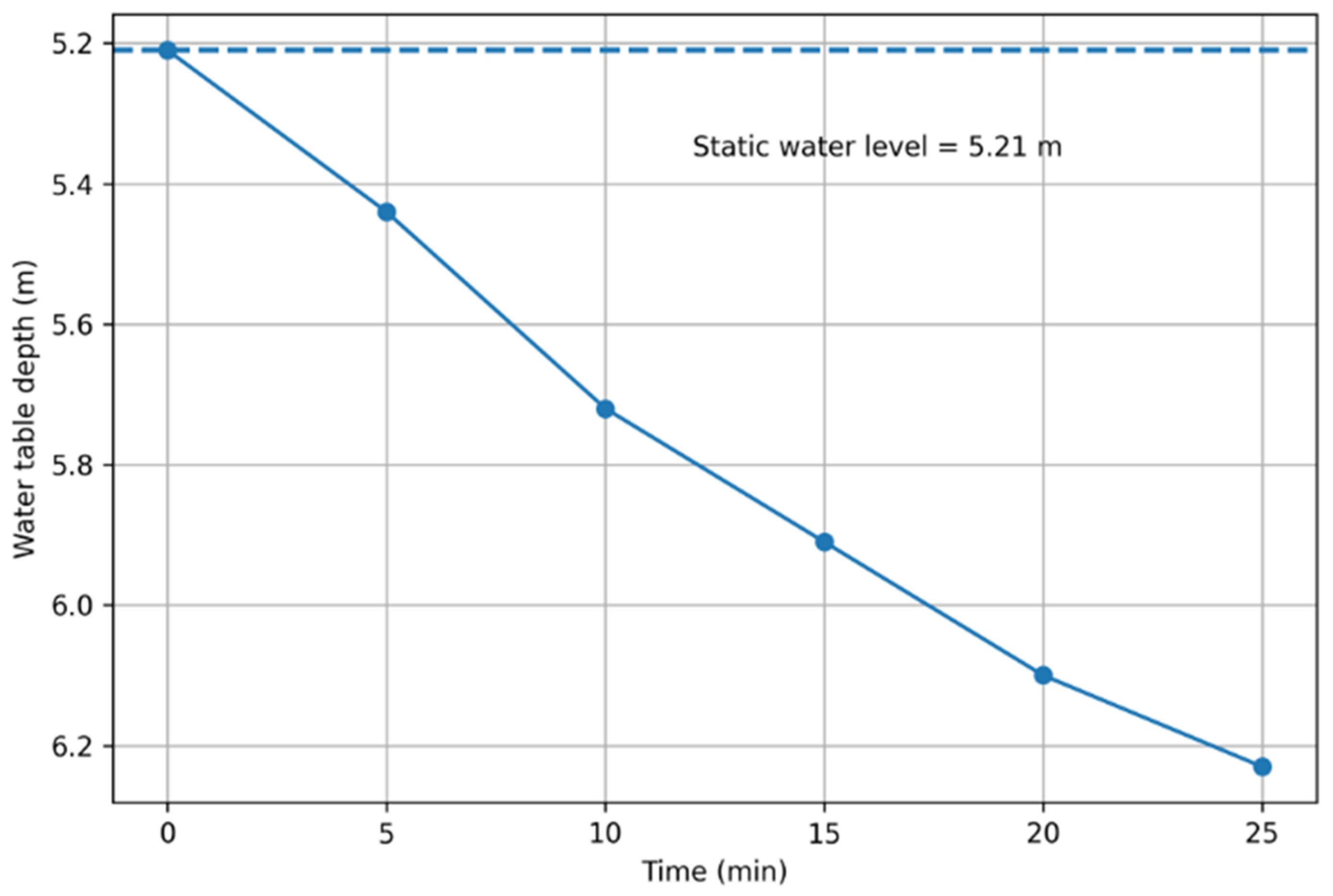
Figure A2. Cooper–Jacob analysis.

Appendix A.2

Figure A3. Stratigraphic profile of the study zone.

Figure A3. Stratigraphic profile of the study zone.

Appendix A.3

Table A1. Adjustment of tidal datum to the study area.

Date (mm/dd/yy)	Hour	Max or Min Value	Tidal Elevation from Tide Gauge Station	Tidal Elevation Transferred to the Study Area (masl)
14 November 2023	15:07	Max	3.31	1.575
12 December 2023	14:51	Max	3.232	1.497
11 January 2024	15:01	Max	3.208	1.473
9 February 2024	15:07	Max	3.246	1.511
9 March 2024	14:45	Max	3.143	1.408
9 April 2024	09:44	Min	1.252	−0.483

Table A1. Adjustment of tidal datum to the study area.

Date (mm/dd/yy)	Hour	Max or Min Value	Tidal Elevation from Tide Gauge Station	Tidal Elevation Transferred to the Study Area (masl)
14 November 2023	15:07	Max	3.31	1.575
12 December 2023	14:51	Max	3.232	1.497
11 January 2024	15:01	Max	3.208	1.473
9 February 2024	15:07	Max	3.246	1.511
9 March 2024	14:45	Max	3.143	1.408
9 April 2024	09:44	Min	1.252	−0.483

References

- Ataie-Ashtiani, B.; Volker, R.E.; Lockington, D.A. Tidal effects on groundwater dynamics in unconfined aquifers. Hydrol. Process. 2001, 15, 655–669. [Google Scholar] [CrossRef] [Scilit]
- Singaraja, C.; Chidambaram, S.; Jacob, N. A study on the influence of tides on the water table conditions of the shallow coastal aquifers. Appl. Water Sci. 2018, 8, 11. [Google Scholar] [CrossRef] [Scilit]
- Purnomo, A.D.; Marfai, M.A.; Husrin, S. Identifying The Effect of Tides on Groundwater Level Fluctuations on Gili Ketapang Island, Indonesia. J. Environ. Eng. Landsc. Manag. 2021, 29, 215–228. [Google Scholar] [CrossRef] [Scilit]
- Yao, D.; Yang, L.; Song, X. Dynamic response of groundwater to rainfall events and sea tides in coral island. Hydrol. Process. 2024, 38, e15254. [Google Scholar] [CrossRef] [Scilit]
- Paule-Mercado, M.C.; Rabaneda-Bueno, R.; Porcal, P.; Kopacek, M.; Matiatos, I.; Huneau, F.; Vystavna, Y. The role of groundwater connectivity in sustaining European lake water systems. Sci. Total Environ. 2025, 994, 180038. [Google Scholar] [CrossRef] [Scilit]
- Toran, L. Groundwater–Surface Water Interaction. In Encyclopedia of Water; Wiley: Hoboken, NJ, USA, 2019; pp. 1–12. [Google Scholar] [CrossRef] [Scilit]
- Fienen, M.N.; Haserodt, M.J.; Leaf, A.T.; Westenbroek, S.M. Simulation of Regional Groundwater Flow and Groundwater/Lake Interactions in the Central Sands, Wisconsin; U.S. Geological Survey: Reston, VA, USA, 2022. [CrossRef] [Scilit]
- Pujades, E.; López, A.; Carrera, J.; Vázquez-Suñé, E.; Jurado, A. Barrier effect of underground structures on aquifers. Eng. Geol. 2012, 145, 41–49. [Google Scholar] [CrossRef] [Scilit]
- Zeng, C.-F.; Chen, H.-B.; Liao, H.; Xue, X.-L.; Chen, Q.-N.; Diao, Y. Behaviours of groundwater and strata during dewatering of large-scale excavations with a nearby underground barrier. J. Hydrol. 2023, 620, 129400. [Google Scholar] [CrossRef] [Scilit]
- Preene, M.; Brassington, R. Potential Groundwater Impacts from Civil-Engineering Works. Water Environ. J. 2003, 17, 59–64. [Google Scholar] [CrossRef] [Scilit]
- Roberts, T.; Preene, M.; Powrie, W. The changing nature of groundwater control for temporary works. Proc. Inst. Civ. Eng.-Civ. Eng. 2023, 176, 11–20. [Google Scholar] [CrossRef] [Scilit]
- Pujades, E.; Jurado, A. Groundwater-related aspects during the development of deep excavations below the water table: A short review. Undergr. Space 2021, 6, 35–45. [Google Scholar] [CrossRef] [Scilit]
- Cashman, P.M.; Preene, M. Groundwater Problems for Excavations in Soils. In Groundwater Lowering in Construction, 3rd ed.; CRC Press: Boca Raton, FL, USA, 2020; pp. 131–164. [Google Scholar]
- Blower, T.; Preene, M. Chapter 3 Problems caused by groundwater. Geol. Soc. Lond. Eng. Geol. Spec. Publ. 2025, 31, 107–144. [Google Scholar] [CrossRef] [Scilit]
- Taylor, C.J.; Alley, W.M. Ground-Water-Level Monitoring and the Importance of Long-Term Water-Level Data; Circular 1217; U.S. Geological Survey: Denver, CO, USA, 2001. Available online: https://pubs.usgs.gov/circ/circ1217/pdf/circular1217.pdf (accessed on 19 November 2025).
- Condon, L.E.; Kollet, S.; Bierkens, M.F.P.; Fogg, G.E.; Maxwell, R.M.; Hill, M.C.; Fransen, H.H.; Verhoef, A.; Van Loon, A.F.; Sulis, M.; et al. Global Groundwater Modeling and Monitoring: Opportunities and Challenges. Water Resour. Res. 2021, 57, e2020WR029500. [Google Scholar] [CrossRef] [Scilit]
- Blower, T.; Preene, M. Chapter 9 Managing groundwater in practice. Geol. Soc. Lond. Eng. Geol. Spec. Publ. 2025, 31, 329–342. [Google Scholar] [CrossRef] [Scilit]
- de Mazatlán, H.A. Reglamento de Construcción de Mazatlán. 2002. Available online: https://www.ordenjuridico.gob.mx/Estatal/SINALOA/Municipios/Mazatlan/MAZREG02.pdf (accessed on 4 January 2026).
- Somerville, S.H. Control of Groundwater for Temporary Works; Construction Industry Research and Information Association: London, UK, 1986. [Google Scholar]
- Huang, C.; Mayer, A.S. Pump-and-treat optimization using well locations and pumping rates as decision variables. Water Resour. Res. 1997, 33, 1001–1012. [Google Scholar] [CrossRef] [Scilit]
- Preene, M.; Loots, E. Optimisation of dewatering systems. In Proceedings of the XVI ECSMGE Geotechnical Engineering for Infrastructure and Development; Winter, M.G., Smith, D.M., Eldred, P.J.L., Toll, D.G., Eds.; ICE Publishing Limited: London, UK, 2015. [Google Scholar] [CrossRef] [Scilit]
- Pujades, E.; De Simone, S.; Carrera, J.; Vázquez-Suñé, E.; Jurado, A. Settlements around pumping wells: Analysis of influential factors and a simple calculation procedure. J. Hydrol. 2017, 548, 225–236. [Google Scholar] [CrossRef] [Scilit]
- Mohammed, O.Y.; Shiekha, A.A. Effect of uncontrolled dewatering on adjacent building. AIP Conf. Proc. 2023, 2651, 020017. [Google Scholar] [CrossRef] [Scilit]
- Ansarifar, M.-M.; Salarijazi, M.; Ghorbani, K.; Kaboli, A.-R. Simulation of groundwater level in a coastal aquifer. Mar. Georesour. Geotechnol. 2020, 38, 257–265. [Google Scholar] [CrossRef] [Scilit]
- Leal-Alves, D.C.; Weschenfelder, J.; Gonzaga, B.A.; Espinoza, J.M.d.A.; Albuquerque, M.d.G.; Ferreira-Cravo, M. Seasonal water table dynamics and effects of a rising sea-level in the low-lying sandy coast of Cassino Beach, southern Brazil. Reg. Stud. Mar. Sci. 2022, 50, 102157. [Google Scholar] [CrossRef] [Scilit]
- Lee, W.-D.; Yoo, Y.-J.; Jeong, Y.-M.; Hur, D.-S. Experimental and Numerical Analysis on Hydraulic Characteristics of Coastal Aquifers with Seawall. Water 2019, 11, 2343. [Google Scholar] [CrossRef] [Scilit]
- Zhou, Y.; Li, W. A review of regional groundwater flow modeling. Geosci. Front. 2011, 2, 205–214. [Google Scholar] [CrossRef] [Scilit]
- Anderson, M.P.; Woessner, W.W.; Hunt, R.J. Applied Groundwater Modeling: Simulation of Flow and Advective Transport; Academic Press: Cambridge, MA, USA, 2015. [Google Scholar]
- Pathak, R.; Awasthi, M.K.; Sharma, S.K.; Hardaha, M.K.; Nema, R.K. Ground Water Flow Modelling Using MODFLOW—A Review. Int. J. Curr. Microbiol. Appl. Sci. 2018, 7, 83–88. [Google Scholar] [CrossRef] [Scilit]
- Thomas, S.D.; French, G.; Watson, J.; Casal, B. Design and modelling for groundwater engineering and control. In Geotechnical Engineering Challenges to Meet Current and Emerging Needs of Society; CRC Press: London, UK, 2024; pp. 2675–2680. [Google Scholar] [CrossRef] [Scilit]
- Langevin, C.D.; Hughes, J.D.; Provost, A.M.; Russcher, M.J.; Panday, S. MODFLOW as a Configurable Multi-Model Hydrologic Simulator. Groundwater 2024, 62, 111–123. [Google Scholar] [CrossRef] [Scilit]
- Ali, M.; Khalil, M.N.; Rehman, F.U.; Farooq, E.O. Hydrogeological Modeling of Aquifer Systems for Sustainable Groundwater Management. Policy Res. J. 2026, 4, 631–639. [Google Scholar] [CrossRef]
- White, J.T.; Fienen, M.N.; Barlow, P.M.; Welter, D.E. A tool for efficient, model-independent management optimization under uncertainty. Environ. Model. Softw. 2018, 100, 213–221. [Google Scholar] [CrossRef] [Scilit]
- Barthel, R.; Banzhaf, S. Groundwater and Surface Water Interaction at the Regional-scale—A Review with Focus on Regional Integrated Models. Water Resour. Manag. 2016, 30, 1–32. [Google Scholar] [CrossRef] [Scilit]
- Srzić, V.; Lovrinović, I.; Racetin, I.; Pletikosić, F. Hydrogeological Characterization of Coastal Aquifer on the Basis of Observed Sea Level and Groundwater Level Fluctuations: Neretva Valley Aquifer, Croatia. Water 2020, 12, 348. [Google Scholar] [CrossRef] [Scilit]
- Itoua-Tsele, C.J.; Tathy, C.; Malonza, D.M. Groundwater Flow Assessment Using Modflow 6 and Model Muse: Application to Pointe-Noire Coastal Aquifers, Congo-Brazzaville. J. Water Resour. Prot. 2021, 13, 900–914. [Google Scholar] [CrossRef]
- Sathish, S.; Chanu, S.; Sadath, R.; Elango, L. Impacts of regional climate model projected rainfall, sea level rise, and urbanization on a coastal aquifer. Environ. Sci. Pollut. Res. 2022, 29, 33305–33322. [Google Scholar] [CrossRef] [Scilit]
- Mathiasen, R.F.; Haugan, E.P.; Andersen, T.R.; Hansen, H.H.; Medhus, A.B.; Poulsen, S.E. Short-Term Ocean Rise Effects on Shallow Groundwater in Coastal Areas: A Case Study in Juelsminde, Denmark. Water 2023, 15, 2425. [Google Scholar] [CrossRef] [Scilit]
- Khosravi, M.; Khosravi, M.H.; Najafabadi, S.H.G. Determining the portion of dewatering-induced settlement in excavation pit projects. Int. J. Geotech. Eng. 2021, 15, 563–573. [Google Scholar] [CrossRef] [Scilit]
- Preene, M.; Roberts, T.O.L. Chapter 8 Groundwater control. Geol. Soc. Lond. Eng. Geol. Spec. Publ. 2025, 31, 299–328. [Google Scholar] [CrossRef] [Scilit]
- Shi, C.; Cao, C.; Lei, M.; Peng, L.; Jiang, J. Optimal design and dynamic control of construction dewatering with the consideration of dewatering process. KSCE J. Civ. Eng. 2017, 21, 1161–1169. [Google Scholar] [CrossRef] [Scilit]
- Sikdar, P.K. Numerical Groundwater Modelling. In Groundwater Development and Management; Springer International Publishing: Cham, Switzerland, 2019; pp. 191–207. [Google Scholar] [CrossRef] [Scilit]
- Reglamento de Construcciones del Distrito Federal. Norma Técnica Complementaria para Diseño y Construcción de Cimentaciones. Ciudad de Mexico. 2023. Available online: https://www.uteycv.esiaz.ipn.mx/comunidad/estructuras/comunicados/NTC%2006.nov.202_cimentaciones.pdf (accessed on 14 July 2025).
- Langevin, C.D.; Hughes, J.D.; Banta, E.R.; Niswonger, R.G.; Panday, S.; Provost, A.M. Documentation for the MODFLOW 6 Groundwater Flow Model; U.S. Geological Survey: Reston, VA, USA, 2017. [CrossRef] [Scilit]
- Winston, R.B. ModelMuse Version 4: A Graphical User Interface for MODFLOW 6; U.S. Geological Survey: Reston, VA, USA, 2019. [CrossRef] [Scilit]
- Instituto Nacional de Estadística y Geografía. Modelo Digital de Elevación Tipo Terreno con 5m de Resolución Derivado de Datos de Sensores Remotos Satelitales y Aerotransportados. F13A45C1. 2015. Available online: https://www.inegi.org.mx/app/biblioteca/ficha.html?upc=889463089599 (accessed on 31 March 2026).
- Comisión Nacional del Agua. Manual de Monitoreo Piezométrico de Acuíferos. México City. 2015. Available online: https://www.gob.mx/cms/uploads/attachment/file/779903/ManualDeMonitoreoPiezometricoDeAcuiferos2008_c.pdf (accessed on 28 February 2026).
- SMN. Universidad Nacional Autónoma de México, Instituto de Geofísica, Servicio Mareográfico Nacional, México. 2025. Available online: https://www.mareografico.unam.mx (accessed on 5 March 2026).
- Instituto Nacional de Estadística y Geografía. Guía Metodológica de la Red Geodésica Vertical. 2017. Available online: https://www.inegi.org.mx/contenidos/productos/prod_serv/contenidos/espanol/bvinegi/productos/nueva_estruc/702825095390.pdf (accessed on 5 March 2026).
- Cueto Díaz, J.d.D.; Heras, J.Z. Estudio de Mecánica de Suelos para un Edificio de 19 Niveles y dos Sótanos, Ubicado Sobre av. del Mar Esq. Calle isla de Chivos, en Mazatlán, Sinaloa. Culiacán, Sinaloa. 2022.
- Subdirección General Técnica Gerencia de Aguas Subterráneas. Actualización de la Disponibilidad Media Anual de Agua en el Acuífero río Presidio (2509), Estado de Sinaloa; Subdirección General Técnica Gerencia de Aguas Subterráneas: Ciudad de México, México, 2024.
- Anomohanran, O.; Iserhien-Emekeme, R.E. Estimation of Aquifer Parameters in Erho, Nigeria Using the Cooper-Jacob Evaluation Method. Am. J. Environ. Sci. 2014, 10, 500–508. [Google Scholar] [CrossRef] [Scilit]
- Ali, H.; Zaman, H.; Biswas, P.; Islam, A.; Karim, N.N. Estimating Hydraulic Conductivity, Transmissibility and Specific Yield of Aquifer in Barind Area, Bangladesh Using Pumping Test. Eur. J. Environ. Earth Sci. 2022, 3, 90–96. [Google Scholar] [CrossRef] [Scilit]
- Servicio Meteorológico Nacional and Comisión Nacional del Agua. Información Estadística Climatológica—Información de Estaciones Climatológicas. Available online: https://smn.conagua.gob.mx/es/climatologia/informacion-climatologica/informacion-estadistica-climatologica (accessed on 4 July 2025).
- MeteoStat. Información de Estación 76459 Mazatlán—El Confital. Available online: https://meteostat.net/es/station/76459?t=2023-10-01/2024-05-31 (accessed on 4 July 2025).
- Mijares, F.J.A. Fundamentos de Hidrología de Superficie; Limusa: México City, México, 2015. [Google Scholar]
- del Distrito Federal, G. Normas Técnicas Complementarias para Diseño y Construcción de Cimentaciones; Academia de la Investigación Científica, A.C.: México City, México, 2004. [Google Scholar]
- Banks, V.J.; Mansour, M.M.; Bricker, S.H.; Lawrence, U.L.; Lelliott, M.R.; Vasu, N.N. Chapter 5 Conceptual models. Geol. Soc. Lond. Eng. Geol. Spec. Publ. 2025, 31, 157–213. [Google Scholar] [CrossRef] [Scilit]
- Thorsen, S. Moon Phases for Mazatlan, Sinaloa, Mexico in 2023. Available online: https://www.timeanddate.com/moon/phases/mexico/mazatlan?year=2023 (accessed on 6 January 2026).
- Thorsen, S. Moon Phases for Mazatlan, Sinaloa, Mexico in 2024. Available online: https://www.timeanddate.com/moon/phases/mexico/mazatlan?year=2024 (accessed on 6 January 2026).
- Hill, M.C.; Tiedeman, C.R. Effective Groundwater Model Calibration; Wiley: Hoboken, NJ, USA, 2007. [Google Scholar] [CrossRef] [Scilit]
- Mai, J. Ten strategies towards successful calibration of environmental models. J. Hydrol. 2023, 620, 129414. [Google Scholar] [CrossRef] [Scilit]
- Razavi, S.; Jakeman, A.; Saltelli, A.; Prieur, C.; Iooss, B.; Borgonovo, E.; Plischke, E.; Piano, S.L.; Iwanaga, T.; Becker, W.; et al. The Future of Sensitivity Analysis: An essential discipline for systems modeling and policy support. Environ. Model. Softw. 2021, 137, 104954. [Google Scholar] [CrossRef] [Scilit]
- Kennedy, D.; Dagon, K.; Lawrence, D.M.; Fisher, R.A.; Sanderson, B.M.; Collier, N.; Hoffman, F.M.; Koven, C.D.; Kluzek, E.; Levis, S.; et al. One-at-a-Time Parameter Perturbation Ensemble of the Community Land Model, Version 5.1. J. Adv. Model. Earth Syst. 2025, 17, e2024MS004715. [Google Scholar] [CrossRef] [Scilit]
- Preene, M. The John Mitchell Lecture 2022: Thinking conceptually about groundwater problems. Q. J. Eng. Geol. Hydrogeol. 2025, 58, qjegh2024-143. [Google Scholar] [CrossRef] [Scilit]
- Panchanathan, A.; Ahrari, A.; Ghag, K.S.; Mustafa, S.; Haghighi, A.T.; Kløve, B.; Oussalah, M. An overview of approaches for reducing uncertainties in hydrological forecasting: Progress and challenges. Earth. Sci. Rev. 2024, 258, 104956. [Google Scholar] [CrossRef] [Scilit]
- Beltrán-Vargas, D.; García-Páez, F.; Martínez-Morales, M.; Rentería-Guevara, S.A. Numerical Models for Groundwater Flows: Key in Construction. In Proceedings of the 8th International Electronic Conference on Water Sciences Session Numerical and Experimental Methods, Data Analyses, Digital Twin, IoT Machine Learning and AI in Water Sciences, Basel, Switzerland, 11 October 2024; Available online: https://sciforum.net/paper/view/18864 (accessed on 4 March 2026).
- Peck, R.B. Advantages and Limitations of the Observational Method in Applied Soil Mechanics. Géotechnique 1969, 19, 171–187. [Google Scholar] [CrossRef] [Scilit]
- Nicholson, D.; Tse, C.-M.; Penny, C. The Observational Method in Ground Engineering: Principles and Applications; CIRIA: London, UK, 1999. [Google Scholar]
- Beltrán-Vargas, D.; García-Páez, F.; Martínez-Morales, M. Numerical Simulation of Water Table Dynamics for Construction Planning in a Coastal Urban Area of Mazatlán, Mexico. In Proceedings of the 6th International Electronic Conference on Applied Sciences, Online, 9–11 December 2025; Available online: https://sciforum.net/paper/view/27815 (accessed on 4 March 2026).
Disclaimer/Publisher’s Note: The statements, opinions and data contained in all publications are solely those of the individual author(s) and contributor(s) and not of MDPI and/or the editor(s). MDPI and/or the editor(s) disclaim responsibility for any injury to people or property resulting from any ideas, methods, instructions or products referred to in the content. |
© 2026 by the authors. Licensee MDPI, Basel, Switzerland. This article is an open access article distributed under the terms and conditions of the Creative Commons Attribution (CC BY) license.