Determination of Material Permeability and Conductivity Based on Electrical Measurements Using FEM and Optimization Methods

Featured Application

Producers of electromagnetic devices are highly dependent on the quality and specifications of the input materials for production. To keep production running continuously and maintain the same output quality, it may be necessary to buy from reserve suppliers or to check every batch of the input material. Sometimes the delivered material is labeled incorrectly and can be a totally different steel. For general devices, the range of accuracy limits is broader. Our paper introduced a method that, using minimal and inexpensive electrical instruments, leverages a model and optimization to detect and evaluate magnetic and electric properties using a contactless approach. The method is ideal for a fast and inexpensive estimate of the material’s permeability and conductivity. The presented approach is unique.

Abstract

Every day, more and more electrical devices are produced, such as electric motors and actuators, which tend to operate according to their intended purpose with minimal maintenance. This is possible if they are assembled with the right input material, which needs to be tested at various stages of production. The presented approach proposes using the existing measuring equipment, combined with the finite element method and an optimization method, to determine the relative permeability and conductivity—in a contactless manner—from electrical measurements for magnetic steel materials. A comparison was made among three models: a whole 3D model, a 1/8 symmetrical 3D model, and a 2D axisymmetric model. During the research, the importance of using a skin-depth mesh was emphasized to obtain the correct results. A novel approach is used to analyze and optimize both the permeability and conductivity using a single model, optimization, and measurements. The optimized Finite Element Model shows very strong model conditioning, as tested with reference data, yielding great results with the measured data.

1. Introduction

In the current era, rapid adaptability in purchasing materials for production from manufacturers’ sites is necessary to maintain uninterrupted production. Producers need to have more suppliers and regular testing of electromagnetic properties to maintain the same quality of their electromagnetic products. Bigger changes can occur for the material with the same standard name from different vendors. It requires more measuring equipment and takes time and effort to prepare the right testing samples. Using a coil with known properties, a power supply, a measuring instrument, and employing electrical parameters in the finite element method (FEM) [1,2] model, along with optimization [3,4,5,6,7,8,9,10,11,12,13,14,15,16,17,18,19,20,21], can drastically ease the process of detecting differences in the properties of the input material for manufacturing. Using the FEM model of the coil and the tested material with optimization, we can determine two key variables for our case: specific conductivity and relative permeability at the tested frequency.

Eddy current testing is already used in many applications to monitor the evolution of steel microstructure during thermal processing, for quality control, for thickness measurement, and for conductivity and permeability [22,23,24,25,26]. Many methods have been developed, such as analytical methods, for calculating eddy currents (e.g., Dodd and Deeds) and associated simplified models, because analytical methods cannot account for all the effects, and the models must be simplified [27,28,29]. The most common eddy current measurement method uses three coils arranged geometrically, with one coil used to excite the magnetic field and the other two to detect it [30,31,32]. There are also two coils [23,28,33] and a single coil approach [21,22,23,24,25,34,35,36], where some use a cylindrical coil, and in [34] they also present a ferrite cored U-shaped sensor [29] which uses an H-shaped coil, and in [23,25,33,35] a planar coil is used, such as in induction cookers.

Multifrequency methods have been developed because, in different frequency ranges, we can acquire different information about the distance between the measuring coil and the mechanical properties. Typically, high-frequency responses are dominated by lift-off variations, whereas lower frequencies provide information about the thickness and electromagnetic material properties. Additionally, pulsed eddy current techniques enable greater penetration depth, allowing for the inspection of thicker or multilayer conductive structures [22,23,25]. Permeability is estimated from the difference between the real and imaginary parts of inductivity and the lift-off guess [26].

Our model was constructed parametrically, so we can change the parameters as needed without creating new models, including multimodel 3D and 2D models [35,37]. We used Ansys Maxwell 2025 R1 because of the higher frequencies; we need to consider the skin effect and penetration depth [38].

Knowing the material’s true electromagnetic properties, such as conductivity and permeability, is key to correctly dimensioning electromagnetic devices, and to determining losses, device efficiency, device dimensions, and required cooling. Knowing the right material properties is especially important for devices that require tight tolerances on deviations from designed values. The efficiency of the electronic power converter, load resistance, and output voltage are significantly influenced by the selected transformer core material [39]. Designers usually consider data provided by the material supplier, which is measured in unprocessed states. In applications such as high-speed permanent magnet synchronous motors (PMSMs), efficiency is highly dependent on material properties [40]. Increasing demand for induction cooking appliances and rising concerns about the materials used for cookware in terms of energy efficiency make this issue increasingly important [41].

Permeability in the region between the Rayleigh and knee regions is approximately constant, then changes in the knee region towards the saturation region. The field used to determine permeability depends on the application. If the device operates under the knee region, a single determination is sufficient. However, if the device operates in the knee region, the process must be repeated several times with different fields, requiring adjustment of the coil’s current. Additional measuring equipment to determine magnetic flux density is not required, as magnetic flux can be obtained from the FEM model.

The measurements were performed at 1000 Hz. The material being tested is usually intended for a device with known usage frequency. It is recommended to perform measurements at the frequency at which the material will be used. If it is used for different frequencies, the process of identifying the material properties can be repeated for each frequency.

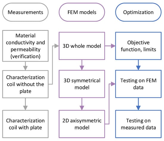
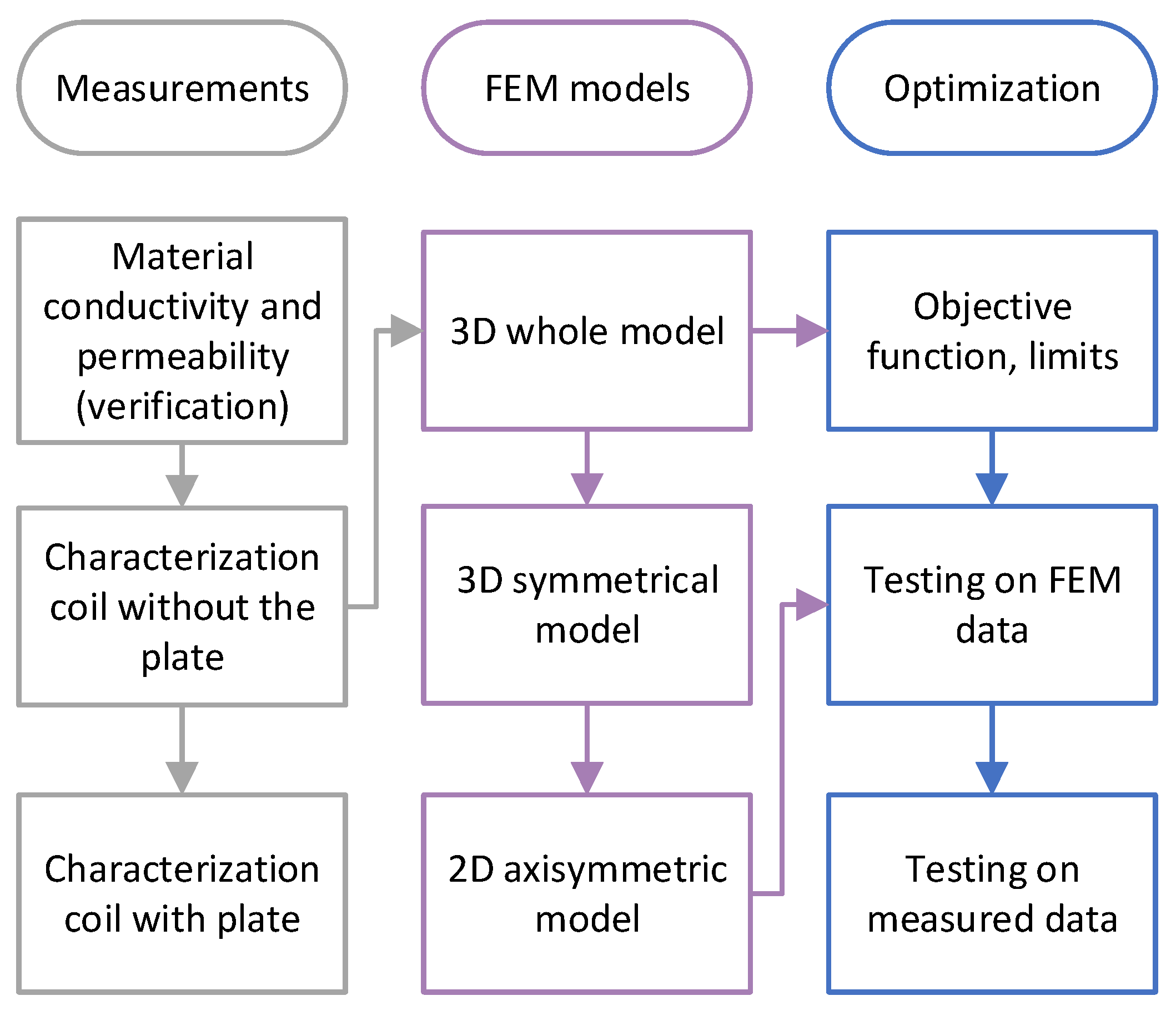
The approach is based on an FEM model, which requires specialized modeling. Because of the AC field and the frequency-dependent penetration depth, it is necessary to adjust the mesh in those regions appropriately. Optimization is used to solve the inverse problem with a direct approach, that is, to determine the unknown material parameters, not to optimize the measurement system or approach. A diagrammatic representation of the used methodology is presented in Figure 1.

Figure 1. Diagrammatic representation of the used methodology.

Our contributions in this work are:

• A multimodel approach, including 3D, 3D symmetrical, and 2D models, was used to assess the differences and the accuracy of the 2D model.
• Consideration and adaptation of the skin-depth mesh width in each iteration, based on the optimization inputs, permeability, and conductivity.
• Using a skin-depth-based mesh is essential, even at entry-level, medium-frequency levels in electrotechnics.
• Since the permeability of low-carbon steel is specified in the producer’s datasheet, it can vary slightly, depending on the applied field, temperature, and production series, and cannot be measured on-site with an instrument. With such an approach, it can be acquired quickly.
• Using already-owned equipment in the laboratory, such as coils and all the used instruments. That means that, with minimal hardware and software, a method can also be implemented using open-source FEM programs.

The paper consists of six Sections. The assembly of the model, the skin mesh, and the measured B-H magnetic curves of the steel plate are described in Section 2. The approach and optimization method are described in Section 3. The results are presented in Section 4, and a brief overview of the process is provided in Section 5. The conclusions are presented in Section 6.

2. Assembly of the Models

2.1. Design and Parametrization

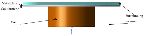
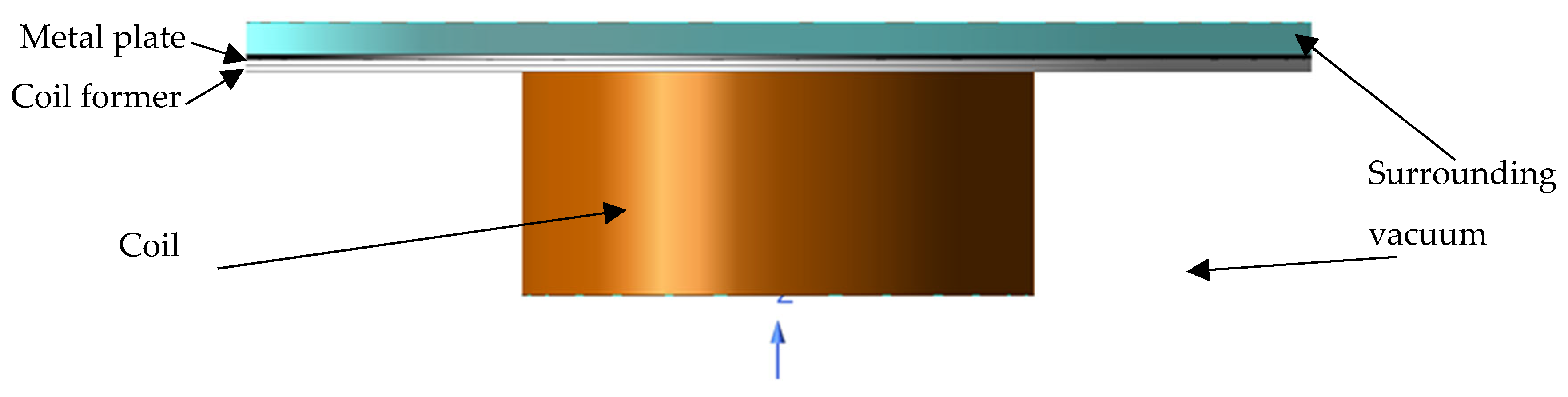
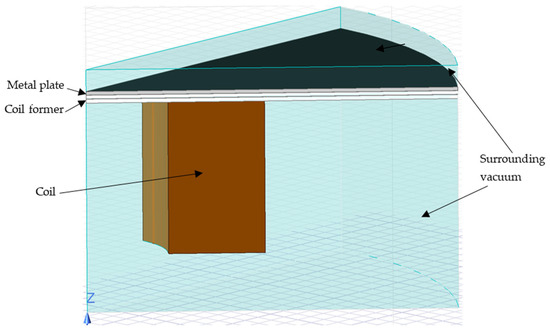
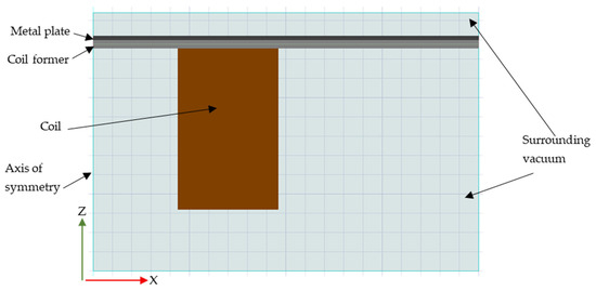
Our goal was to design an accurate, modular FEM model that can be adjusted parametrically for different plate frequencies, thicknesses, and diameters, as well as electrical currents and other parameters. We created three different models to compare their accuracy and the time required to complete the simulations. Because the model is symmetrical, we created the 3D whole model shown in Figure 2, the 1/8 3D Symmetrical Model shown in Figure 3, and the 2D axisymmetric model shown in Figure 4. The whole 3D model in Figure 2 is displayed without the visible layer of surrounding vacuum in the lower part to present the coil better.

Figure 2. The whole 3D model and the material properties used.

Figure 3. The 1/8 symmetrical 3D model and the material properties used.

Figure 4. The 2D axisymmetric model and the material properties used.

The model is composed of a copper coil winding, a metal plate, an air gap between the coil and the plate, and surrounding air, as shown in Table 1.

Table 1. Model components and materials.

Model Component	Material
Coil	Copper
Metal Plate	Used low-carbon steel
Coil Former	Polyethylene Terephthalate (PET)

The presented approach is very flexible and supports the use of different dimensions of coils, plates, and power supplies. We recommend using round samples to create a 2D axisymmetric model for faster analysis. Dimensions used in our case are: an internal coil radius of 20 mm, an external radius of 50 mm, and a length of 46 mm. The distance between the coil and the plate is 2.2 mm, which is the distance of the plastic coil former. The distance of the plastic former is divided into two parts, each 1.1 mm thick, to increase the mesh density. A plate is placed on top of the coil former with a thickness of 1 mm and a radius of 100 mm. Around those elements is a surrounding vacuum on the lower side of the coil former, with a height of 57.8 mm, and on the top of the plate, with a height of 6 mm, both with a radius of 100 mm. Around the model, a region is placed with dimensions of 30 mm in height and 120 mm in radius on the lower side of the coil former, and 17 mm in height and 120 mm in radius on the top of the plate. With these dimensions, we have ensured that the entire field lies within the model’s area.

2.2. Generation of the Mesh and Skin-Depth Mesh

As mentioned before, the mesh density is essential for obtaining accurate results from the calculations. Maxwell Ansys automatically refines the mesh during the solution process to improve accuracy. When considering applications at higher frequencies, it is important to account for skin effect and skin depth, and to increase the mesh density in that region. Considering these, we tried different approaches and, in the end, used a Maxwell skin-depth mesh refined according to the optimized conductivity and permeability, calculated in every iteration of optimization using Equation (1) with the actual input values.

$$\delta =\sqrt{{\displaystyle \frac{\rho }{\pi f{\mu }_r{\mu }_0}}}$$

(1)

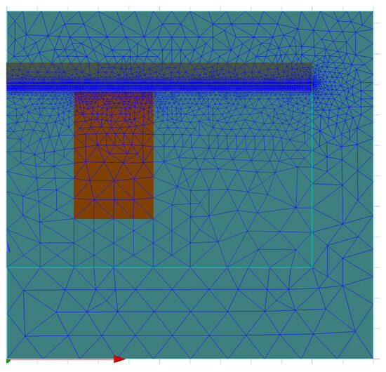
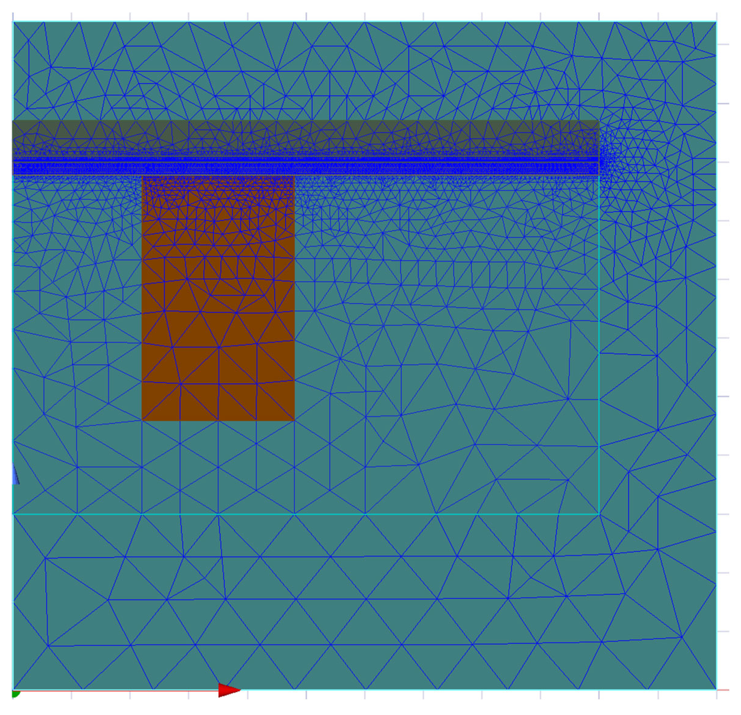
To increase density in the coil former near the plate, we added length-based mesh, which slightly improved accuracy and field distribution in the plate. The adaptive, skin-depth, and length-based meshes are shown in Figure 5.

Figure 5. The 2D meshed model with adaptive, length-based, and skin-depth meshes.

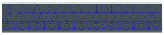
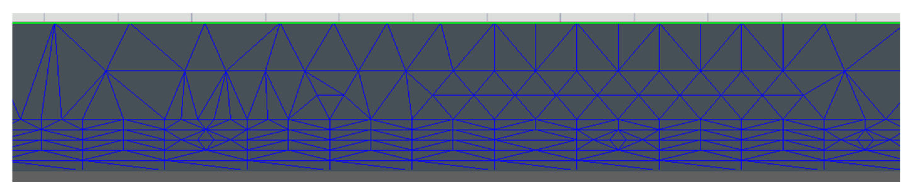
On the plate, we have five layers of mesh in the area of the skin–effect penetration depth, as shown in Figure 6.

Figure 6. Density of the skin-depth mesh in the metal plate.

2.3. Measured Material Properties

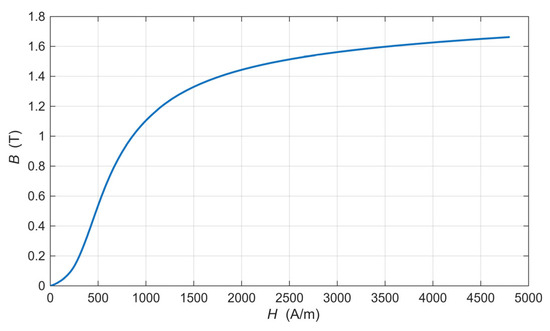
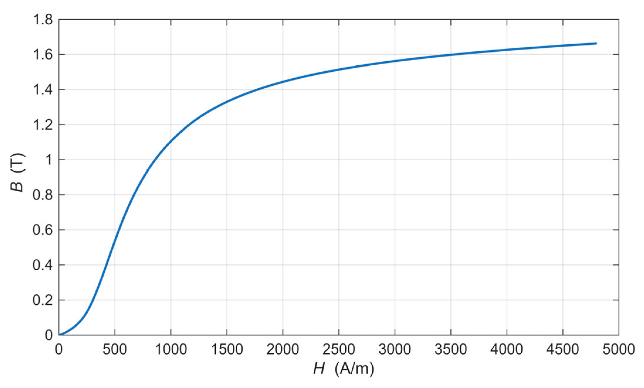
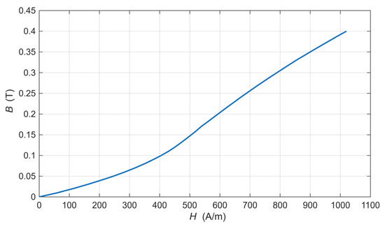
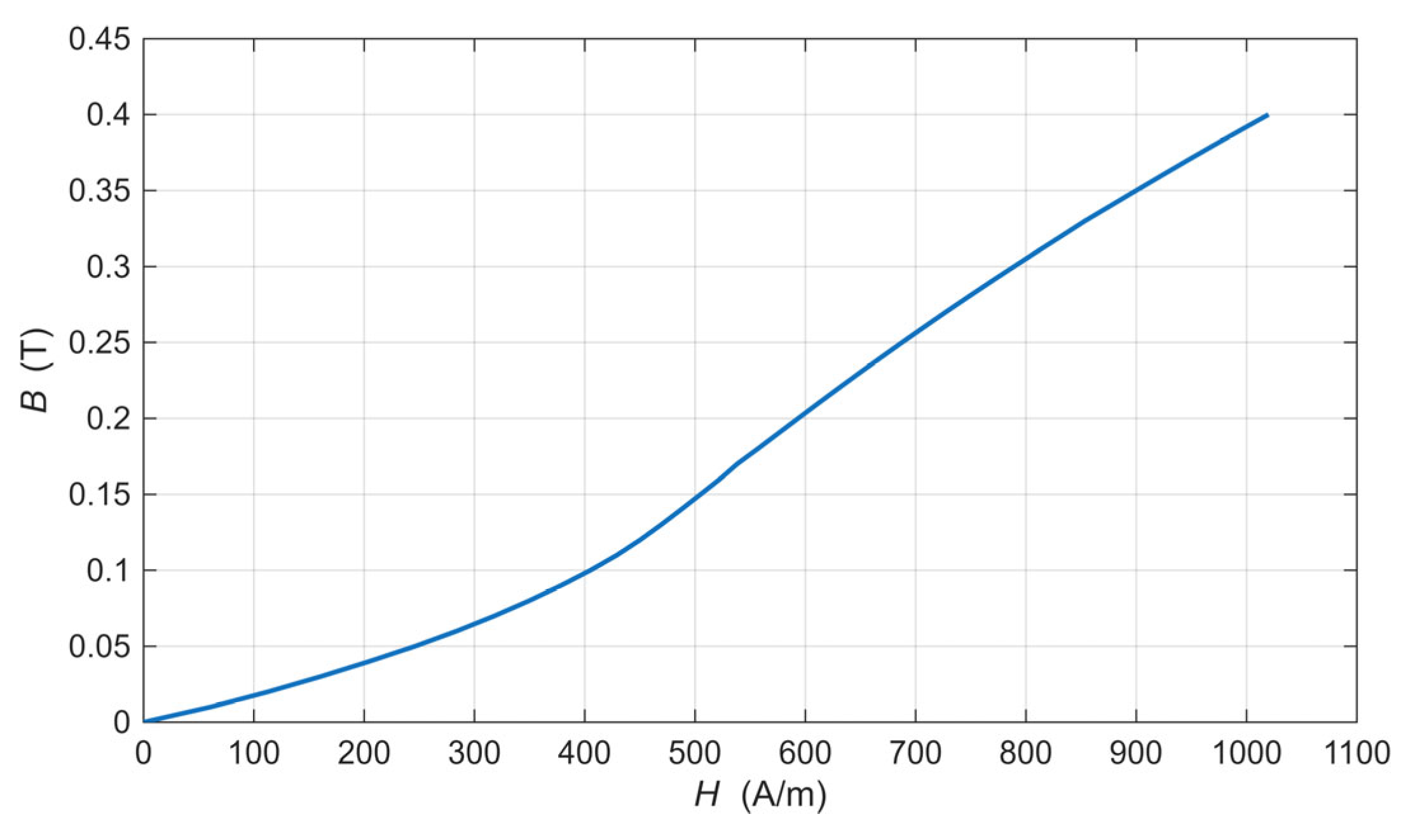
For the tested material, we measured the static magnetization curve at the selected frequency. Figure 7 presents the static magnetization curve measured with an applied direct current (DC) field, and Figure 8 presents the magnetization curve at the selected frequency with an alternating current (AC) field. Because our tested material is used at higher frequencies, we measured and ran the optimization at a frequency of 1000 Hz.

Figure 7. Static magnetization curve of the used low-carbon steel.

Figure 8. Magnetization curve of the used low-carbon steel at 1000 Hz.

From the B-H magnetics curves, we can calculate the relative permeability (2):

$${\mu }_r={\displaystyle \frac{B}{{\mu }_{0}H}}$$

(2)

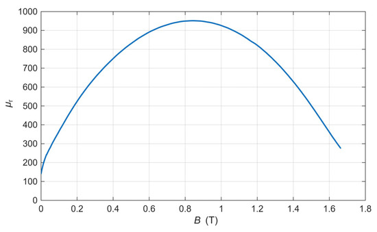
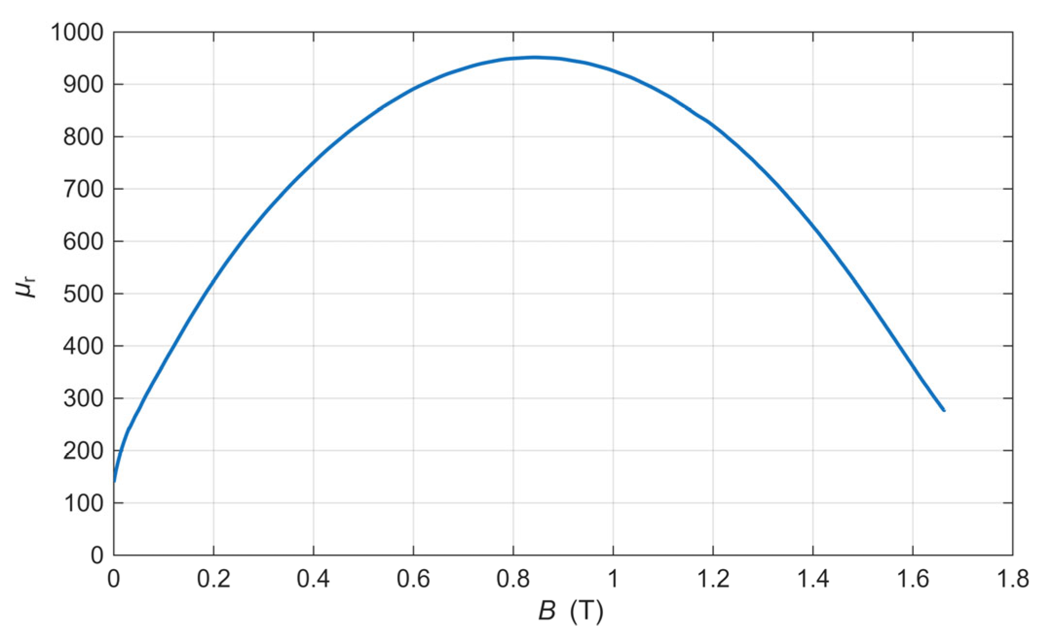
Using that equation, we obtain the relative permeability as a function of the applied magnetic flux. From the static curve, we obtain the intrinsic permeability, which we measured over a wider range, such as 1.6 T, as shown in Figure 9.

Figure 9. Intrinsic permeability curve of the used low-carbon steel.

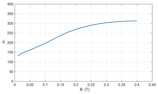
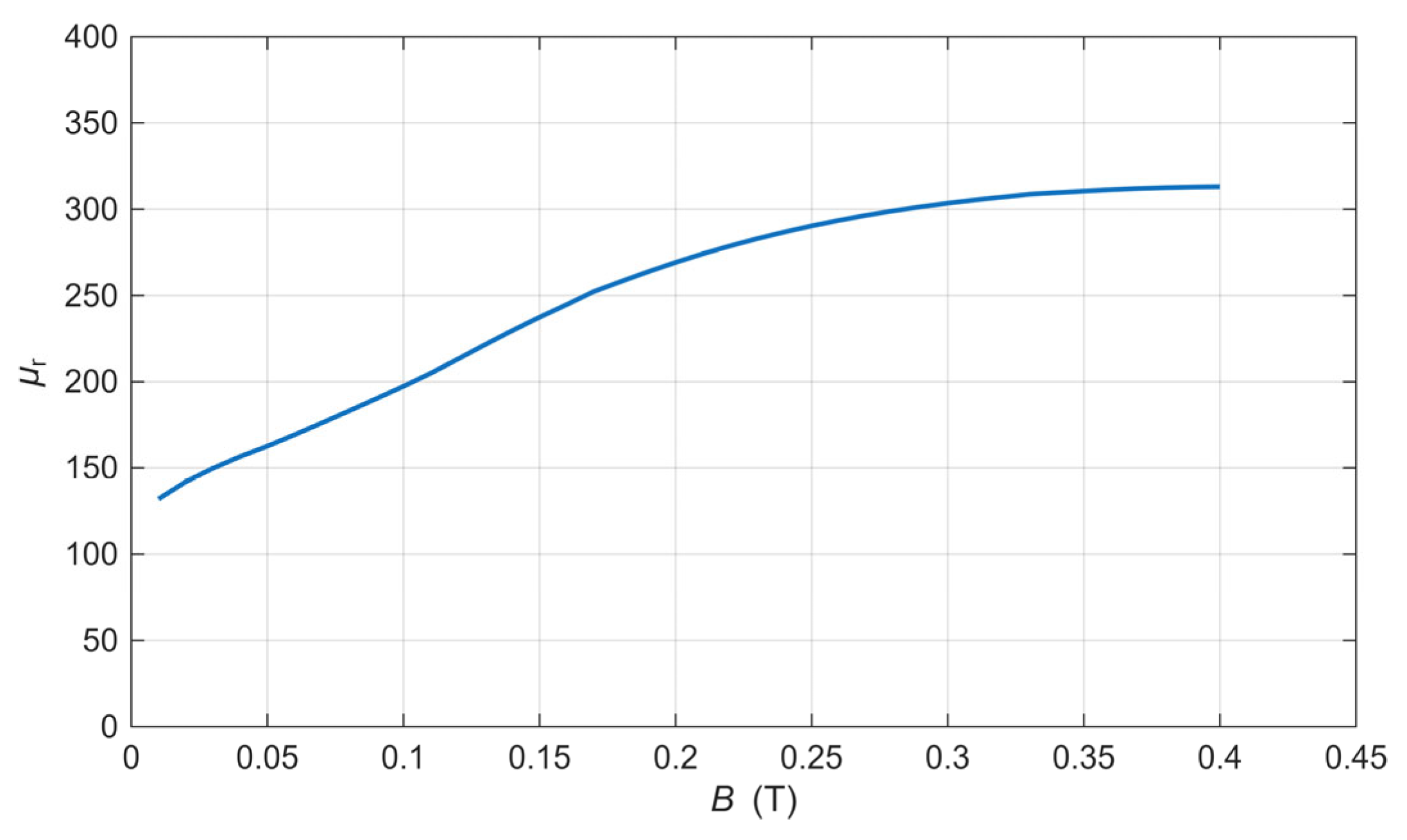
The effective permeability of the material at 1000 Hz was decreased due to saturation effects induced by the eddy currents, as shown in Figure 10. To mitigate the significant heating associated with these currents, the measurements were limited to 0.4 T. In our application, the permeability does not exceed this limit, as the material exhibits saturation behavior that limits further enhancement of the magnetic response.

Figure 10. Effective permeability curve of the used low-carbon steel at 1000 Hz.

3. Approach and Optimization Method

3.1. Approach and FEM Analysis

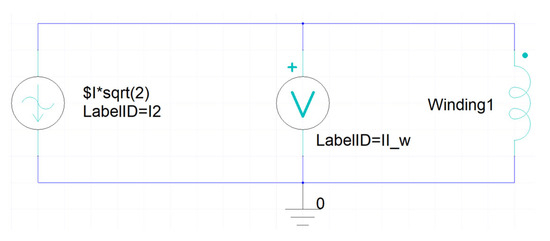
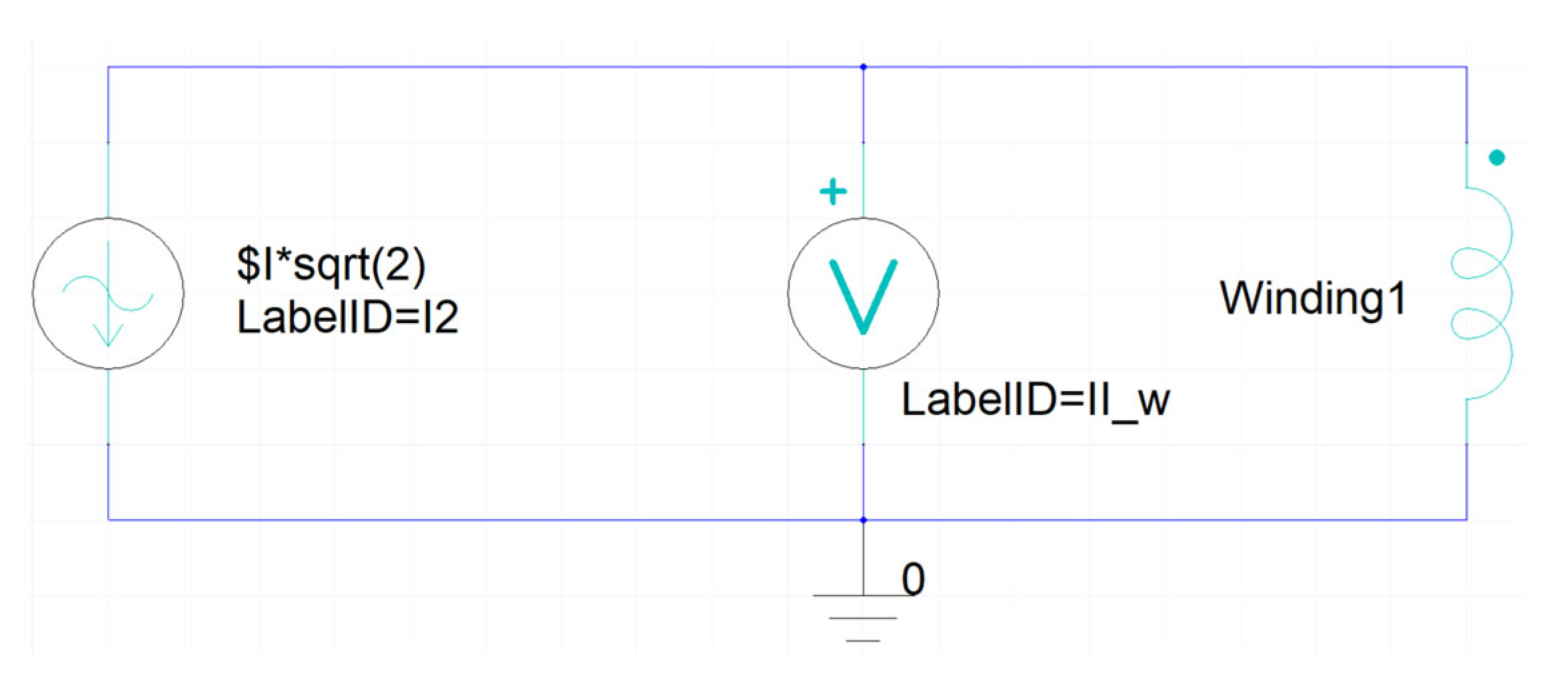
Because of the relatively thin metal plates, similar to skin depth, which would be measured using this method, and to shorten the calculation times significantly, we assumed permeability as a scalar value. The Maxwell Circuit was used to create a simple electrical circuit with a current power source, a winding, and a voltmeter. The circuit was created to analyze the coil as a winding, because of the electrical parameters Ansys calculates, such as induced voltage, flux linkage, coil current, and a matrix that calculates resistance and inductance automatically. We measured the exact voltage on the coil with a voltmeter. The coil was defined as a stranded wire conductor. Figure 11 presents the circuit created in the Maxwell Circuit.

Figure 11. We used a circuit created in a Maxwell Circuit.

Boundary conditions and initial conditions for the whole 3D model, according to Ansys 2025 R1, were set to default, meaning no specific boundary conditions are specified for the surface. The following two treatments are assigned based on surface position. For the boundaries between the objects, Natural boundaries were used, which describe the natural variation between objects. For the external boundaries of the solution domain, a Neumann boundary condition was used.

For the 1/8 symmetrical 3D model, an Independent/Dependent boundary was used. That boundary condition enables us to analyze only one period of the periodic structure. Magnetic fields at the Independent and Dependent boundaries match each other with a set number of symmetries. We analyzed 1/8 of the model, which means analyzing only one part, then multiplying the symmetry by 8.

For the 2D axisymmetric model, a Balloon boundary condition was used, with the region outside the drawing space treated as an infinitely large domain. Magnetic flux lines are neither tangent nor normal to the boundary. The axis of symmetry was along the Z-axis, as shown in Figure 4.

The optimization method code was implemented in Matlab 2025a, connected to Ansys Maxwell for the FEM analysis. A connection between Matlab and Ansys was made using a COM port.

3.2. Reference Values Used for Optimization

The reference value of plate permeability was selected based on the measured magnetic flux near the plate during the coil measurements and the intrinsic permeability curve of the used low-carbon steel (Figure 9). Based on the measured values, we set the assumed reference relative permeability to 300, as shown in Table 2. The limits of plate conductivity were set based on the measurements of the resistance of the used low-carbon steel plate at known dimensions and thickness, using the four-wire method. The conductivity at room temperature is around 6,600,000 S/m, so we used this value as a reference.

Table 2. Reference values of steel plate permeability and conductivity.

Reference Values	Value
Permeability of the Plate µr	300
Conductivity of the Plate σ (S/m)	6,600,000

Permeability is non-linear, meaning it depends on magnetic flux. To analyze other magnetic fields, we need to repeat the measurements at different current values.

3.3. Verification of the FEM Model with the Measurements

Verification of the FEM model against real problem measurements is very important to ensure correct analysis. We did it as presented in Figure 1 (the boxes on the left under the “measurements”). We measure material properties, such as conductivity and permeability, using precise laboratory measurement equipment. The plate’s conductivity was measured in a laboratory using the four-wire method. Relative permeability was obtained as a function of the applied magnetic flux density by measuring the B-H magnetization curve at 1000 Hz. Based on the magnetic flux density measured near the plate, we determined the relative permeability to be around 300.

We measure and characterize the coil without the plate. Using this procedure, we measured the coil losses, which are mostly in the copper winding. Measured were electrical parameters, including coil current, effective voltage, and coil loss power. We did the same in the FEM simulation, simulating only the coil losses. In FEM simulations for this scenario, we set the plate’s conductivity to 0 S/m and its relative permeability to 1, corresponding to air’s permeability. Table 3 presents the results and differences between the real problem and the FEM simulation.

Table 3. Characterization of the measurements of the coil without the steel plate and the FEM model.

Parameter	Measured Value	FEM Simulation Value
Coil Current (A)	0.488	0.488
Effective Voltage (V)	169.831	173.067
Loss Power (W)	1.251	1.113

We continued verification and compared measurements of the real problem with the FEM model using reference permeability and conductivity values (Table 2). We measured the coil current, voltage, and power loss when a steel plate was placed on the coil. We did the same with the FEM model using reference parameters. Because in real problems we cannot measure the separate losses of the coil and the plate, we subtract the coil’s loss power without the plate from the coil’s measured loss power with the plate. Table 4 presents the results and differences between the real problem and the FEM simulation. The measured coil current of 0.488 A was set into the FEM model as an input value. The effective voltage and loss power are the results of the simulation and should be similar to the measured values. Based on the data in Table 4, the differences in effective voltage was 1.7%, and the difference in plate loss power was 2.1%. We observe relatively small differences and conclude that the verification against the real problem and the FEM model is correct.

Table 4. Characterization of the measurements of the coil with the steel plate and the FEM model.

Parameter	Measured Value	FEM Simulation Value
Coil Current (A)	0.488	0.488
Effective Voltage (V)	197.416	200.69
Plate loss Power (W)	7.452	7.297

The same was made before the optimization to see if the model is well-conditioned for optimization. More about that is explained in Section 4.2.

3.4. Optimization Method

Two parameters were optimized using the Differential Evolution (DE) method to identify the minimum of the objective function (OF). The DE/rand/1/exp strategy was employed to search for candidate solutions. The factors for the DE stepsize (F) and the crossover probability (CR) were selected based on prior experience [11,12], resulting in values of F = 0.6 and CR = 0.8. The number of iterations (ITs) was set to IT = 100, and the population size was set to NP = 10. We ran the optimization ten times with the same number of IT. The optimized parameters were permeability and conductivity. The limits of the plate permeability are set based on the effective permeability curve, where the lower limit (100) was lower than the calculated minimal value, and the upper limit (800) was much higher than the saturation value. We set this upper limit so high to see whether the problem always returns the correct values after the selected IT number. We set limits within a broader range of plate conductivity based on the reference values from Table 4 and on iron’s conductivity. The set limits are within a broader range, from the lower limit (2,000,000) to the upper limit (10,000,000). The parameter limits are shown in Table 5.

Table 5. Optimization parameters’ limits.

Parameter	Lower Limit	Upper Limit
Permeability of the Plate µr	150	800
Conductivity of the Plate σ (S/m)	2,500,000	9,000,000

DE stars with variation written by (3) for DE/rand/1/exp

$$v_i^{\left(g\right)}=x_{r1}^{\left(g\right)}·\left({\mathrm{x}}_{\mathrm{r}2}^{\left(g\right)}-x_{r3}^{\left(g\right)}\right)$$

(3)

Crossover follows the variation, and it is made by (4).

$$u_i^{\left(g\right)}=\left\{\begin{array}{c}{v}_{i,j}^{\left(g\right)} if r_j\le CR \mathrm{o}\mathrm{r} j=j_{rand} \\ x_{i,j}^{\left(g\right)} \mathrm{o}\mathrm{t}\mathrm{h}\mathrm{e}\mathrm{r}\mathrm{w}\mathrm{i}\mathrm{s}\mathrm{e}\end{array}\right.$$

(4)

The last step is selection (5), and a new population is obtained.

$$x_i^{\left(g+1\right)}=\left\{\begin{array}{c}{u}_i^{\left(g\right)} \mathrm{i}\mathrm{f} f\left(u_i^{\left(g\right)}\right)\le f\left(x_i^{\left(g\right)}\right) \\ x_{i,j}^{\left(g\right)} \mathrm{o}\mathrm{t}\mathrm{h}\mathrm{e}\mathrm{r}\mathrm{w}\mathrm{i}\mathrm{s}\mathrm{e}\end{array}\right.$$

(5)

The lower-case u, v, and x represent the population members.

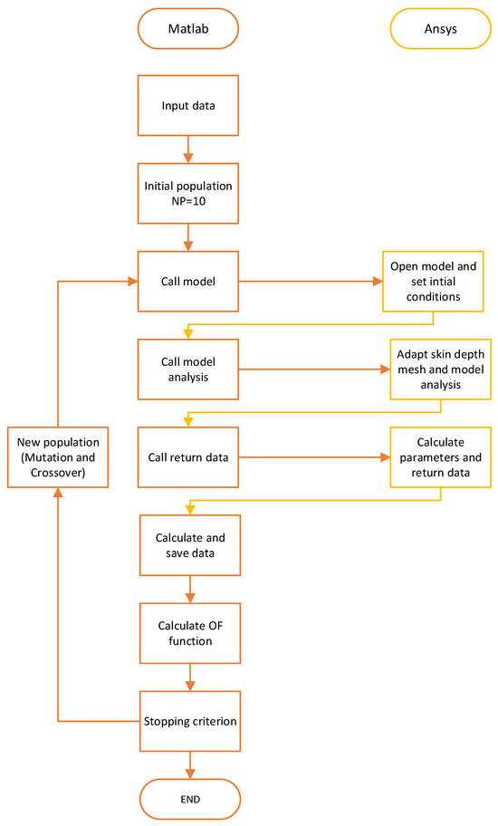
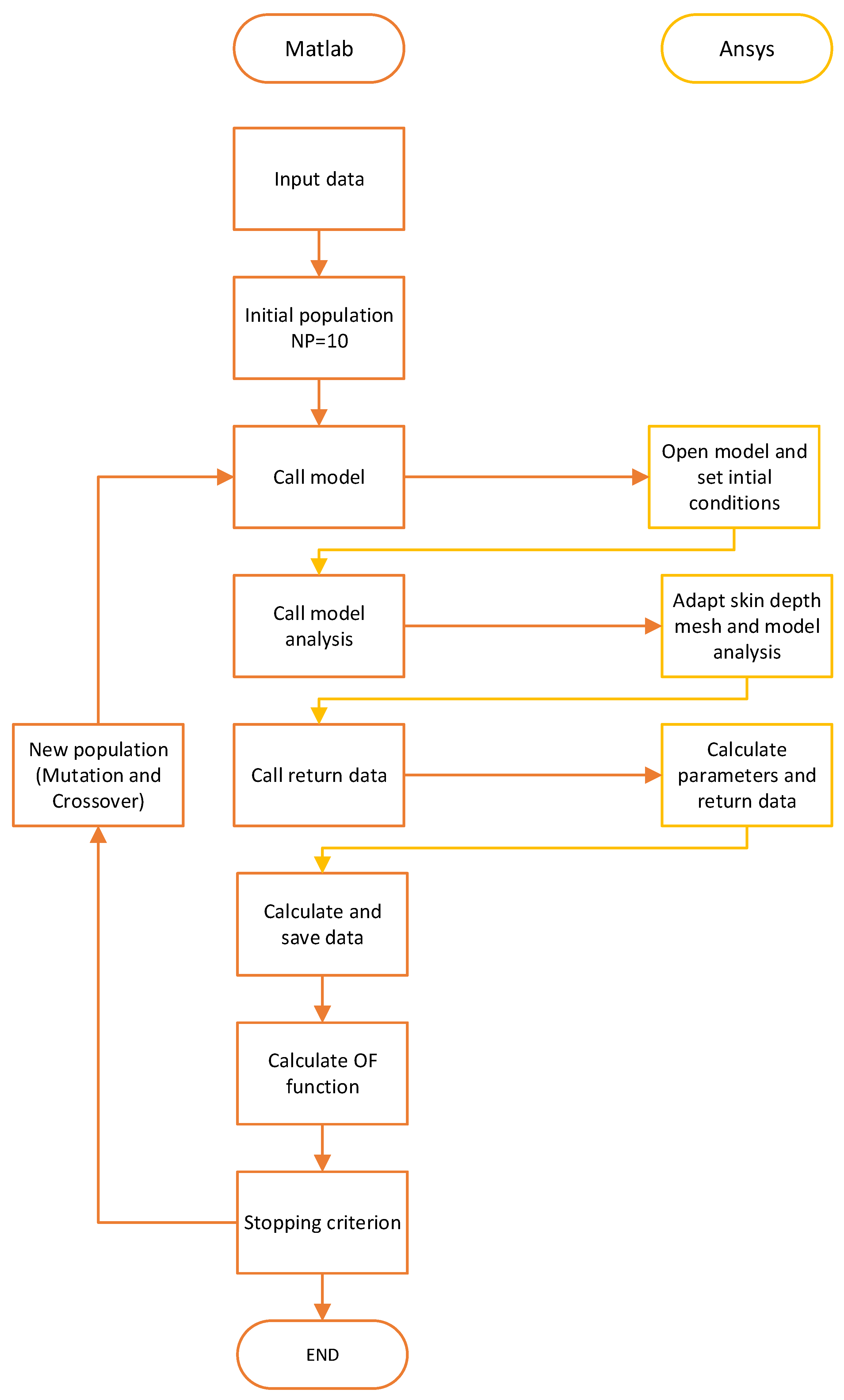
The workflow and connection between Maxwell and Ansys are shown in Figure 12. We can see that, after initialization in Matlab with input data and an initial population, we call the Model in Ansys. The initial population was created within the boundary values using the random function, then we called the Ansys model and set the initial condition. After that, we performed skin-depth mesh refinement based on the input permeability and conductivity parameters, along with model analysis. After the analysis, we called again to receive the calculated data in Ansys, which will, later, be processed in Matlab and the calculated OF. If the stop criteria are not met, we continue with mutations and crossover of the input data until the stop criteria are met.

Figure 12. Flowchart of the connection between Matlab and the Ansys algorithm.

3.5. Objective Function

The objective function was based on the measured electrical parameters and the model’s input parameters. Using a constant-current source, we measured the coil’s voltage and power. They were our parameters for the OF: U_m is the Ansys model’s effective voltage, U_me is the measured effective voltage, and U_ref is the reference effective voltage, selected based on Ansys model calculations to dissipate power in the plate (6). Because both are important and are correlated with the electrical current, we selected the same weight of 0.5, as shown in Table 6.

Table 6. Objective function parameters’ weight values.

Weight	Value
$w_1$—Effective Voltage	0.5
$w_2$—Plate loss Power	0.5

$$OF=w_1{{\left({\displaystyle \frac{U_m-U_{me}}{U_{ref}}}\right)}^2+w_2\left({\displaystyle \frac{P_m-P_{me}}{P_{ref}}}\right)}^2$$

(6)

3.6. Calculation of Power, Voltage, and Verification

Ansys automatically calculates some variables, such as solid and stranded losses. In our case, solid losses occurred in the metallic plate, and stranded losses occurred in the coil winding. The voltages calculated in Ansys are presented in real and imaginary parts, so they need to be converted to effective values for comparison with the measured values (7). Verification was performed by comparing the calculated values with the measured values. The coil winding losses were measured by applying the same current to the coil and subtracting the impedance of the supply wires. As mentioned before, that value needs to be close to the calculated stranded losses. The plate and coil losses were measured in the same way, except for the coil windings, which represent solid losses.

$$U_{eff}={\displaystyle \frac{\sqrt{U_{re}^2+U_{im}^2}}{\sqrt{2}}}$$

(7)

4. Results

4.1. Comparison of the Different Models’ Analysis Results and Analysis Time

Table 7 presents a comparison between the three different models listed in 2.1. Whole 3D, 3D symmetrical, and 2D models. We compared the solid losses and effective voltage between the different mesh setups, with and without the skin-depth mesh. The initial mesh in Ansys was set to auto, with the dynamic surface resolution set to fine or large. That was the most important parameter to be as close as possible to the measurements. In addition to the effective voltage measured on the coil, matching these two shows that our model reflects the real conditions with these parameters. We ran 10 analyses for each scenario, using random input data for permeability and conductivity within the parameter limits listed in Table 5. The values for solid losses and voltages are presented for reference, with a relative permeability of 300 and a conductivity of 6,600,000 S/m (Table 4). Based on that, we calculated the average analysis time for each scenario. The solver setup was set to a maximum of 20 passes, 1 percent error, and convergence to 30 percent refinement per pass, with a minimum of 2 passes. The stranded losses in Ansys are automatically calculated and do not depend on differences in permeability or conductivity.

Table 7. Comparison of 3D, 3D symmetrical and 2D model analysis results.

Model	Skin Mesh Layers	Number of Passes	Number of Tethraedra	Energy Error (%)	Solid Loss (W)	Effective Voltage (V)	Average Time (sec)
3D	0	3	11,908	0.749	0.123	207.006	63
	2	7	109,886	0.921	5.622	195.868	534
	5	14	851,975	0.680	6.434	194.922	2237
3D symmetrical	0	8	58,587	0.877	3.662	191.278	197
	2	5	54,525	0.795	5.867	191.142	182
	5	7	165,952	0.695	6.190	190.736	486
2D	0	11	4733	0.580	7.515	197.044	28
	2	6	17,160	0.699	7.461	197.367	46
	5	3	14,285	0.827	7.452	197.416	39

The results show that a 3D model without a skin mesh has a relatively small average analysis time, but produces very poor results in terms of solid loss. From this, we can conclude that Ansys does not automatically account for skin depth in such scenarios, and users should be aware of this. Including a two-layer skin mesh, we can see that the number of tetrahedra and the average analysis time increased almost tenfold. There is still a difference in solid loss compared to the measured values when the effective voltage is close to the measured value. When using a five-layer skin-depth mesh, we came closer to the measured values with solid losses, but were slightly lower in effective voltage than in the previous scenario. We also increased the mesh across the whole model and came really close to the measured values, but the analysis times were unreasonable, especially for optimization.

The results for the 3D symmetrical model in our case show it to be the worst available option, as the analysis times are quite long due to the large number of tetrahedra required on each symmetry surface. In the first scenario, without using a skin mesh, we saw better results for solid losses than for the 3D model, but we used a fairly large initial skin mesh, a larger number of passes, and a longer analysis time. We expect that such a symmetric model for our scenario will reduce the analysis time slightly and yield results comparable to those from the full 3D model.

For the 2D model in the first scenario without a skin mesh, we observed a high number of passes, quite accurate solid losses, and an effective voltage. Compared to the previous scenarios, Ansys generated a much larger mesh for a much smaller analyzed object. Using skin mesh values, solid losses, and effective voltage, the results slowly approached the measured values. When the five-layer skin mesh analysis time was lower than two layers, and compared to other scenarios, we can conclude that, in such a problem, the most important factor for accuracy is a refined skin mesh.

From the results in Table 7, we can conclude that 2D is sufficiently accurate for optimization. Optimizations using evolutionary methods require a large number of objective function evaluations; in our case, 1000 for each determination of material parameters. The FEM calculation time depends on the number and type of finite elements. Thus, the calculation is significantly faster for an axisymmetric calculation than for a 3D calculation.

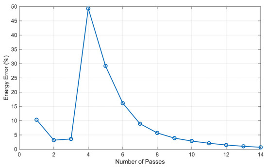
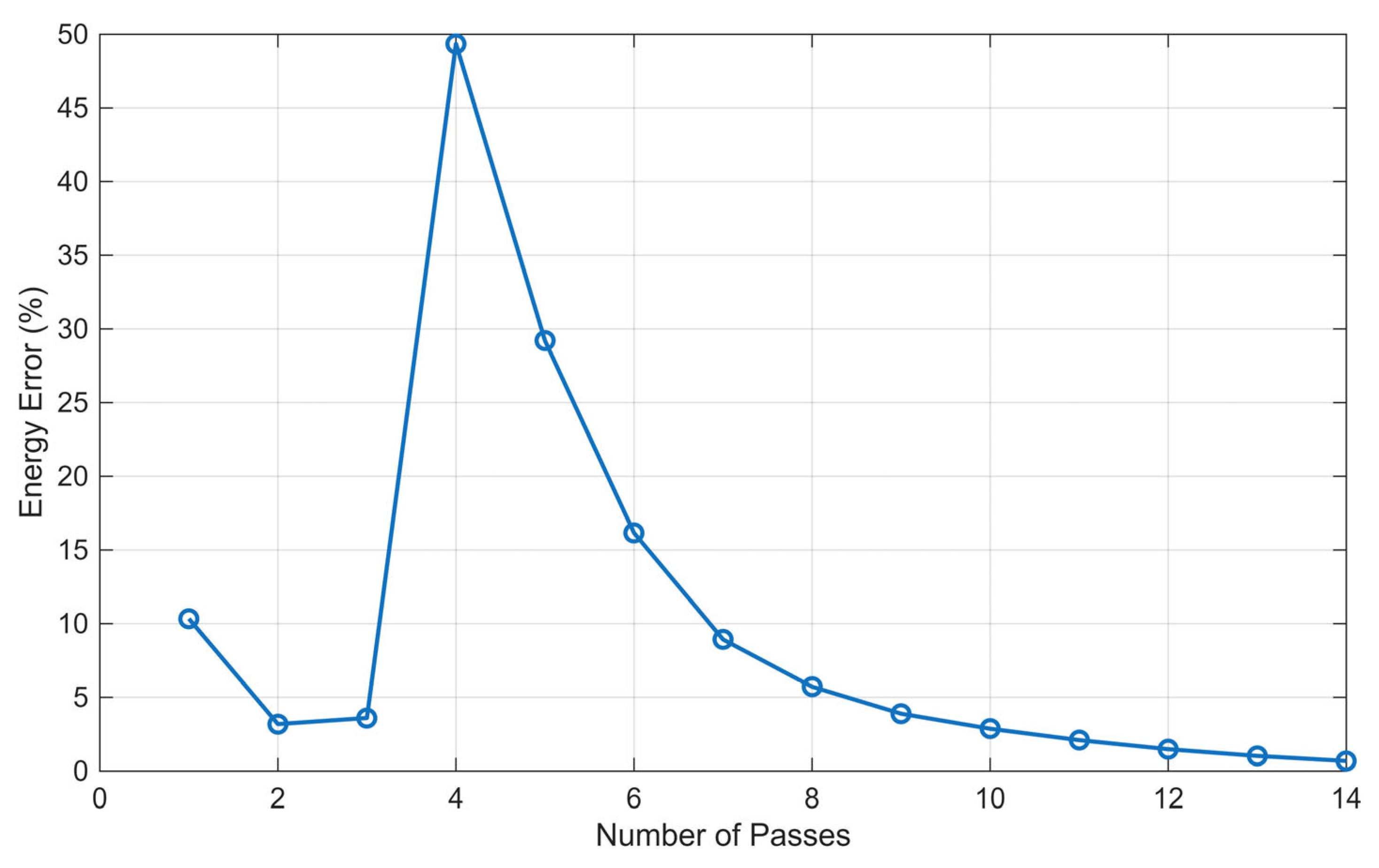
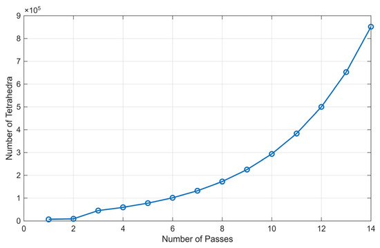
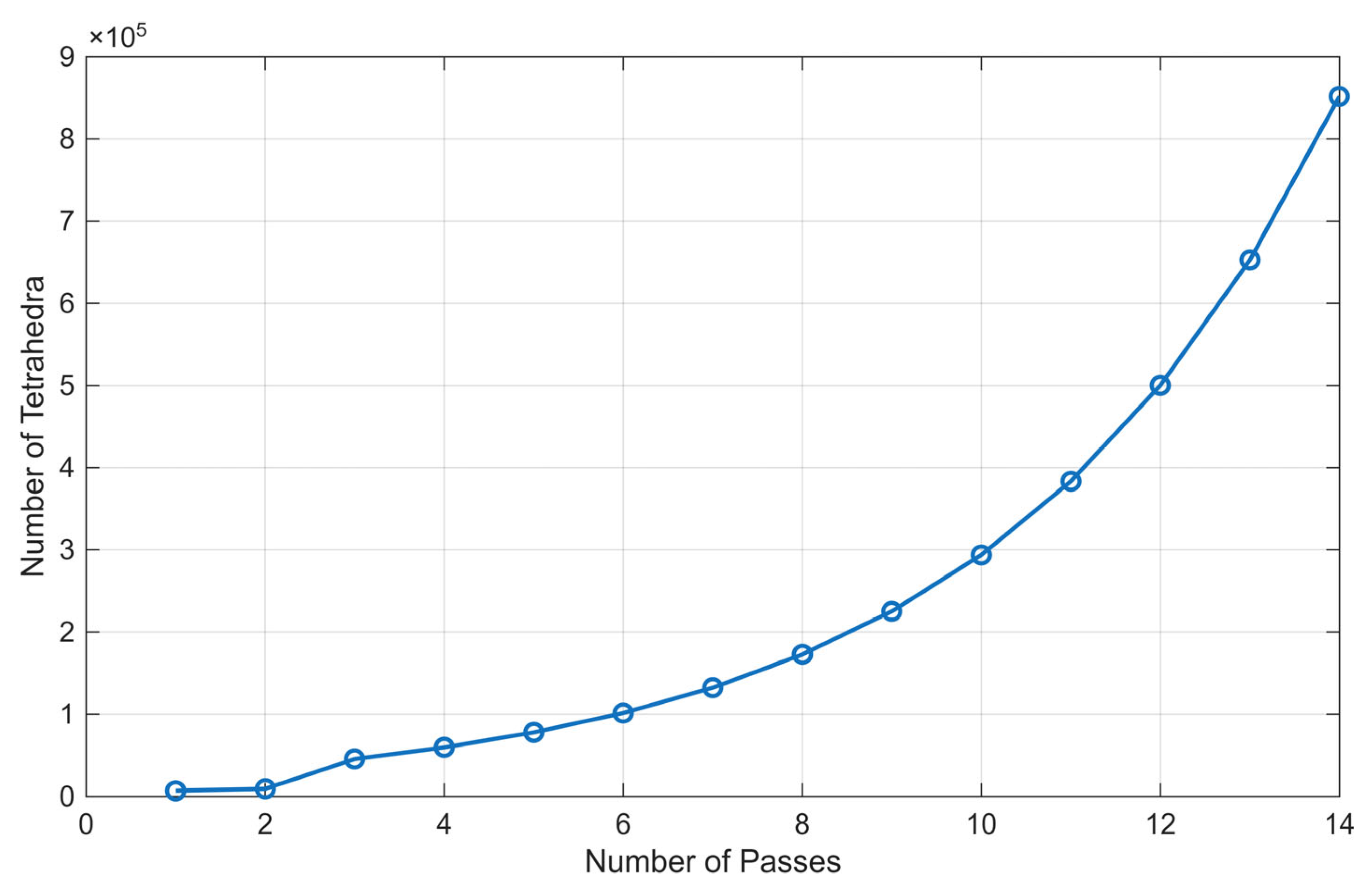
Figure 13 presents the energy error during analysis of the 3D model as a function of the number of solver passes. At the fourth pass, we see a larger spike, and, after each pass, the error decreased until it reached an energy error below 1 percent. Figure 14 shows the number of tetrahedral mesh elements per pass, which increased exponentially. The number of tetrahedra is important for accuracy, but it increases the computation time.

Figure 13. Energy error during analysis for a 3D model with a five-layer skin-depth mesh.

Figure 14. Number of tetrahedra during the analysis for a 3D model with a five-layer skin-depth mesh.

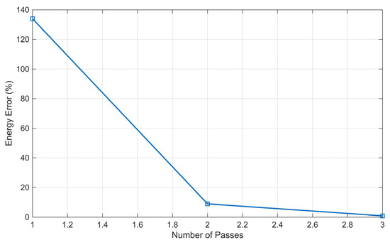
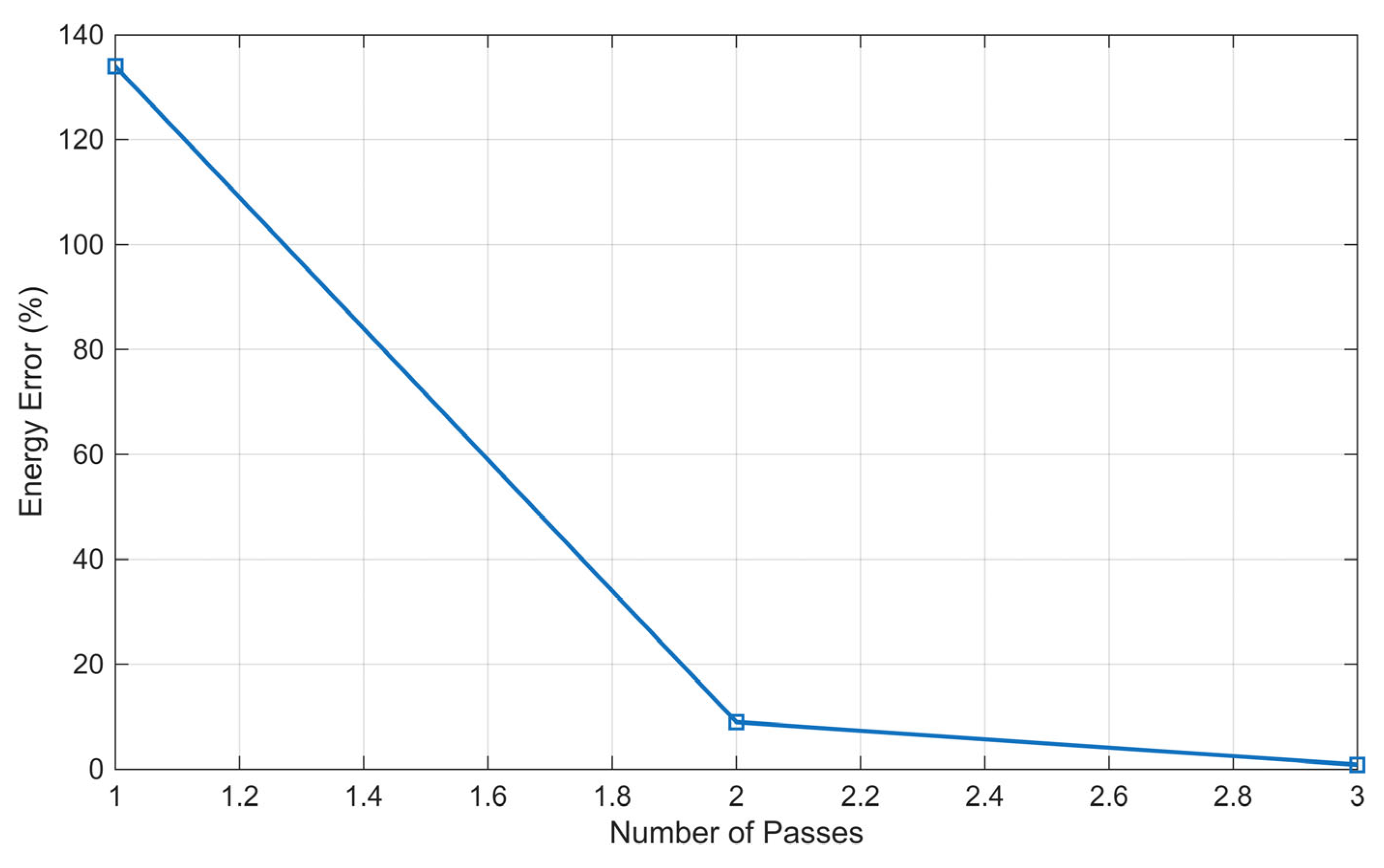
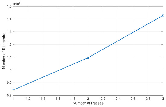
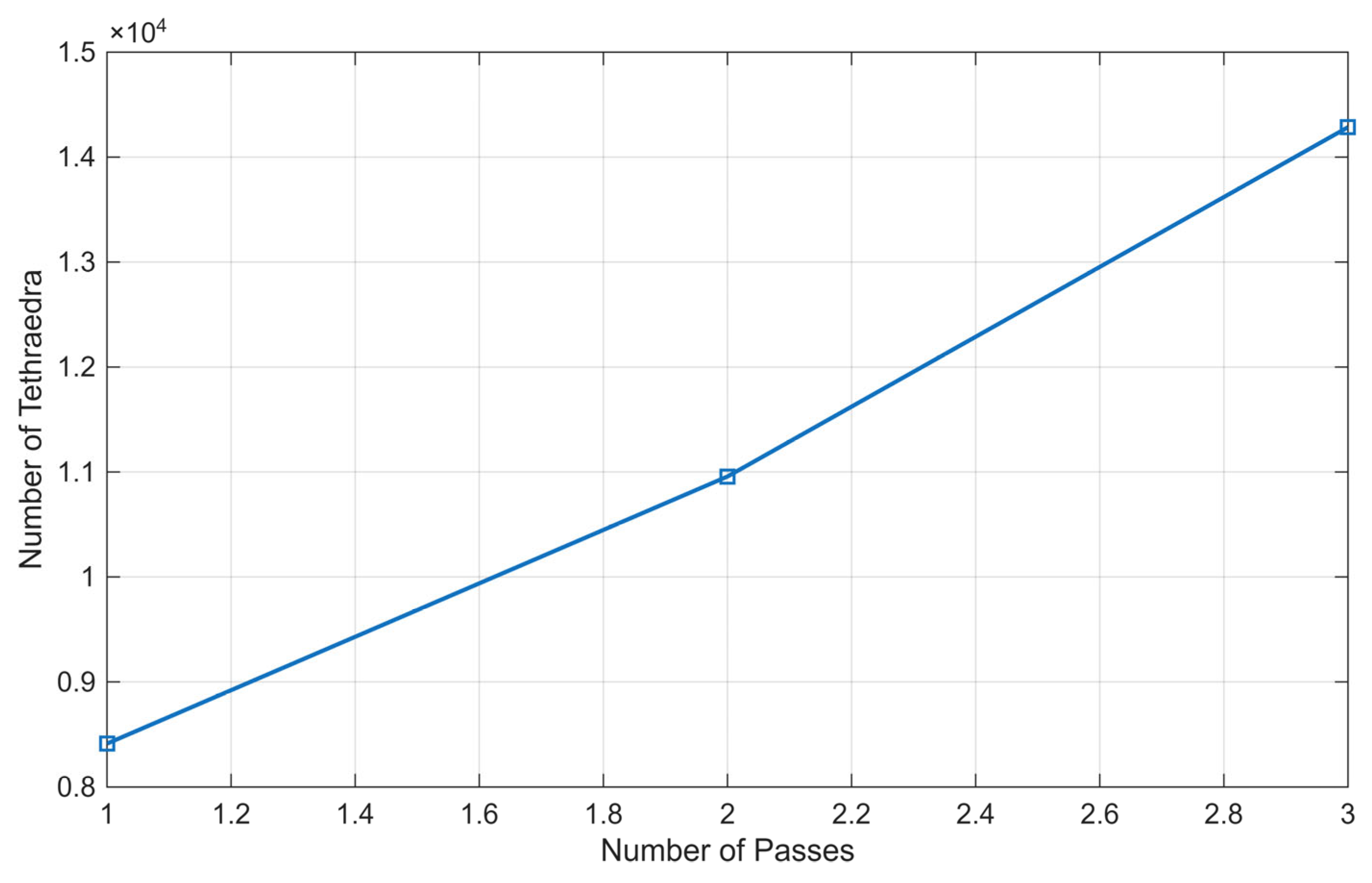
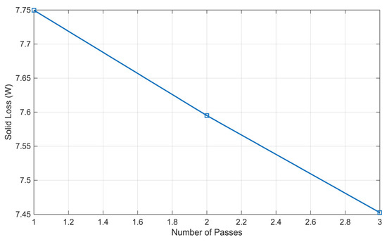
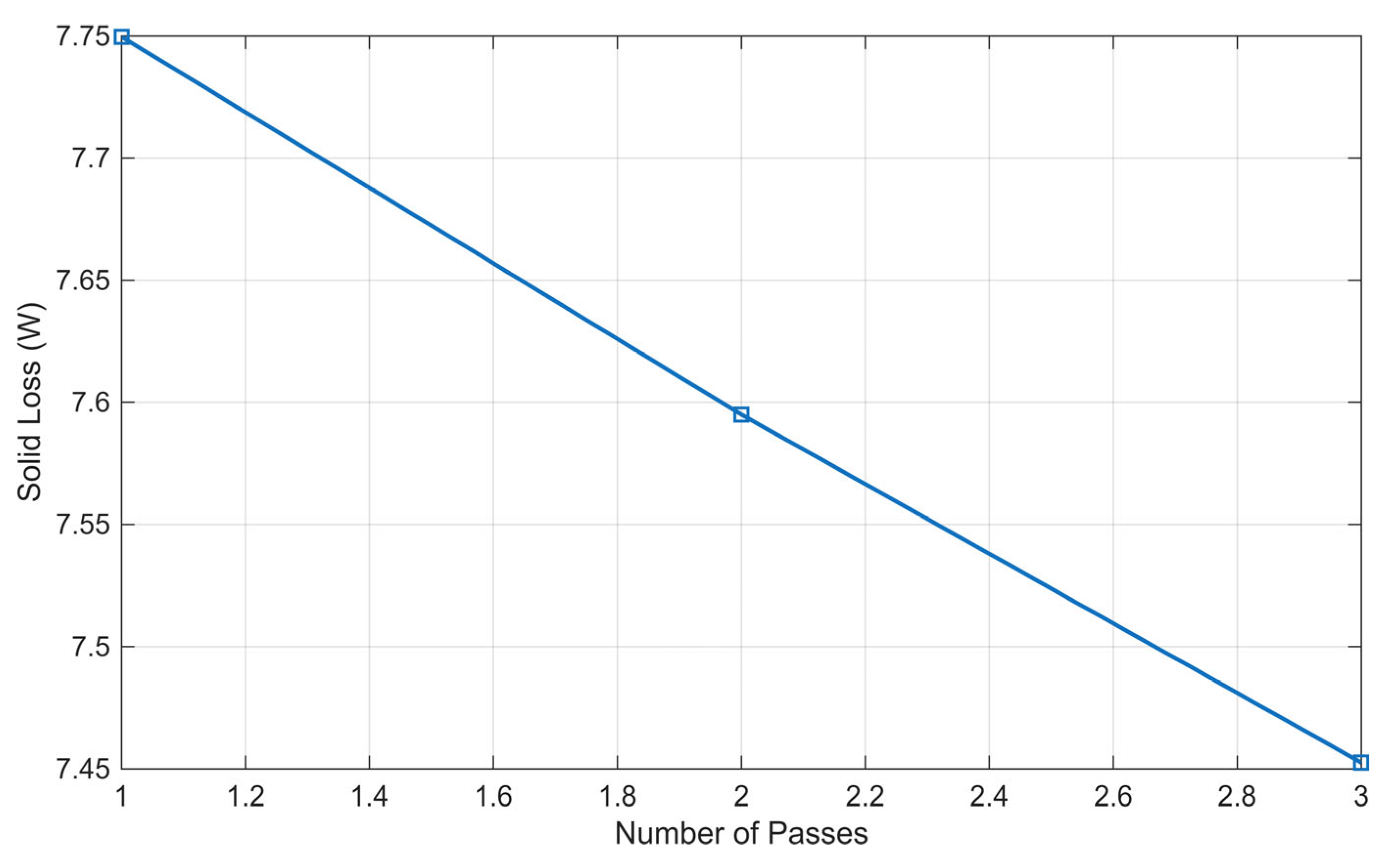
For the 2D, five-layer skin-depth model, we observed different behavior due to only 3 passes. Figure 15 shows the energy error as a function of passes, and we see a slightly higher first-pass error that decreased quickly to under 1% by the third pass. The number of tetrahedra elements increased from 8412 to 14,285, as shown in Figure 16. Changes in the solid loss or steel plate loss between the passes are shown in Figure 17. Compared to the increase in tetrahedra elements, we can conclude that, within the current range, the reference value for the correlated measured one increases with the tetrahedra elements.

Figure 15. Energy error during analysis for 2D model with a five-layer skin-depth mesh.

Figure 16. Number of tetrahedra during analysis for 2D model with a five-layer skin-depth mesh.

Figure 17. Solid loss change during analysis of the 2D model with a five-layer skin-depth mesh.

4.2. Results of the Optimizations Using the FEM Reference Analysis Input Data

Before we started the optimization based on the measured data, we checked the model’s conditionality using the reference parameters (Table 4) and FEM analysis results (Table 8). We used the same OF and parameters; only the measurement parameters were set to the reference values. We made 5 runs, and, based on reference values, the mean OF value was $3.188\times {10}^{-29},$ which we considered as a well-conditioned problem. Since there are no measurement errors in this approach, the calculated conductivity and permeability were identical to those used in the FEM model. This confirms the approach is correct.

Table 8. Reference FEM model analysis results based on plate reference values.

FEM Simulation Parameters	Value
Effective Voltage (V)	197.416
Plate loss Power—Solid loss (W)	7.452
Coil Current (A)	0.488

The differences between the reference input data, results of the optimization using the FEM reference analysis, and the results of the optimization using the FEM reference analysis are shown in Table 9. The differences in the values of permeability are seen at the seventh decimal, and of the conductivity at the second decimal.

Table 9. Reference values of the steel plate compared to the results of the reference analysis input data.

Parameter	Reference Value	Optimized Value
Permeability of the Plate µr	300	300.00000016
Conductivity of the Plate σ (S/m)	6,600,000	6,600,000.038

4.3. Results of the Optimizations Using the Measured Input Data

After we confirmed that the problem was well-conditioned and that the optimization was running as expected, we used the measured data. The measured data used for the optimization are presented in Table 10. The analyses were run 10 times, with 100 iterations per optimization run, for a total of 10,000 analyses. For the optimization analysis, we used a workstation with an Intel Xeon W-2245 processor (3.90 GHz) and 64 GB of random-access memory with a total analysis time of around 10 days.

Table 10. Measured coil data with the steel plate.

Measured Parameters	Value
Effective Voltage (V)	200.69
Plate loss Power (W)	7.297
Coil Current (A)	0.488

In Table 11, the analysis results are presented for four parameters: the OF value, Relative Permeability, Conductivity, and the time for each analysis, where we have best value (B), worst value (W), mean value (M), standard deviation (SD), highest value (H), and lowest value (L).

Table 11. Analysis results using the measured input data for 10 independent runs.

Parameters		Value
OF	B	7.514 × 10−5
	W	7.513 × 10−5
	M	7.513 × 10−5
	SD	5.833 × 10−10
Relative Permeability	H	293.488
	L	292.448
	M	293.033
	SD	0.481
Conductivity (S/m)	H	6,240,726
	L	6,218,796
	M	6,231,127
	SD	10,142.21
Time for each analysis (s)	H	153.511
	L	29.372
	M	84.114
	SD	42.041

Based on the results in Table 11 for OF, the difference between B and W is small and changes to the least decimals, as seen in the values of M and SD. There, we can also confirm good conditionality and robustness of the DE optimization method.

The difference between the H and L values of relative permeability is only around 1, with a mean of 293 and an SD of 0.481. Compared to the reference value of relative permeability of 300, this is around 2.3%.

The fluctuations between the H and L values of conductivity are slightly higher with SD 10,142 S/m and M 6,231,127 S/m. There is also a larger difference compared to the measured conductivity value in Table 4, around 5.5%, which we considered acceptable for our case.

The time for each analysis run ranged from H 153 s (the longest) to L 29 s (the fastest), with M 84 s. Differences can occur when saving the data and when the same value has already been calculated. That is most common after the OF stops changing, and the input parameters are close or identical.

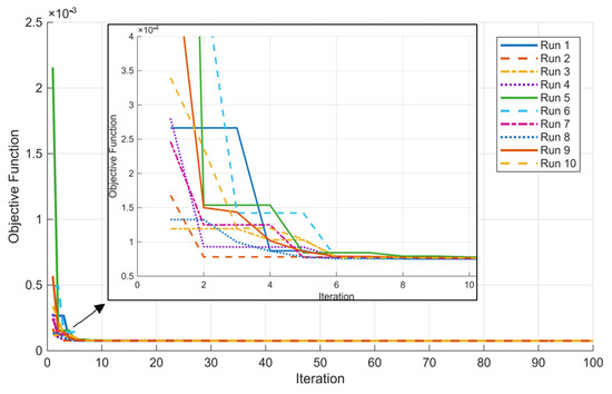
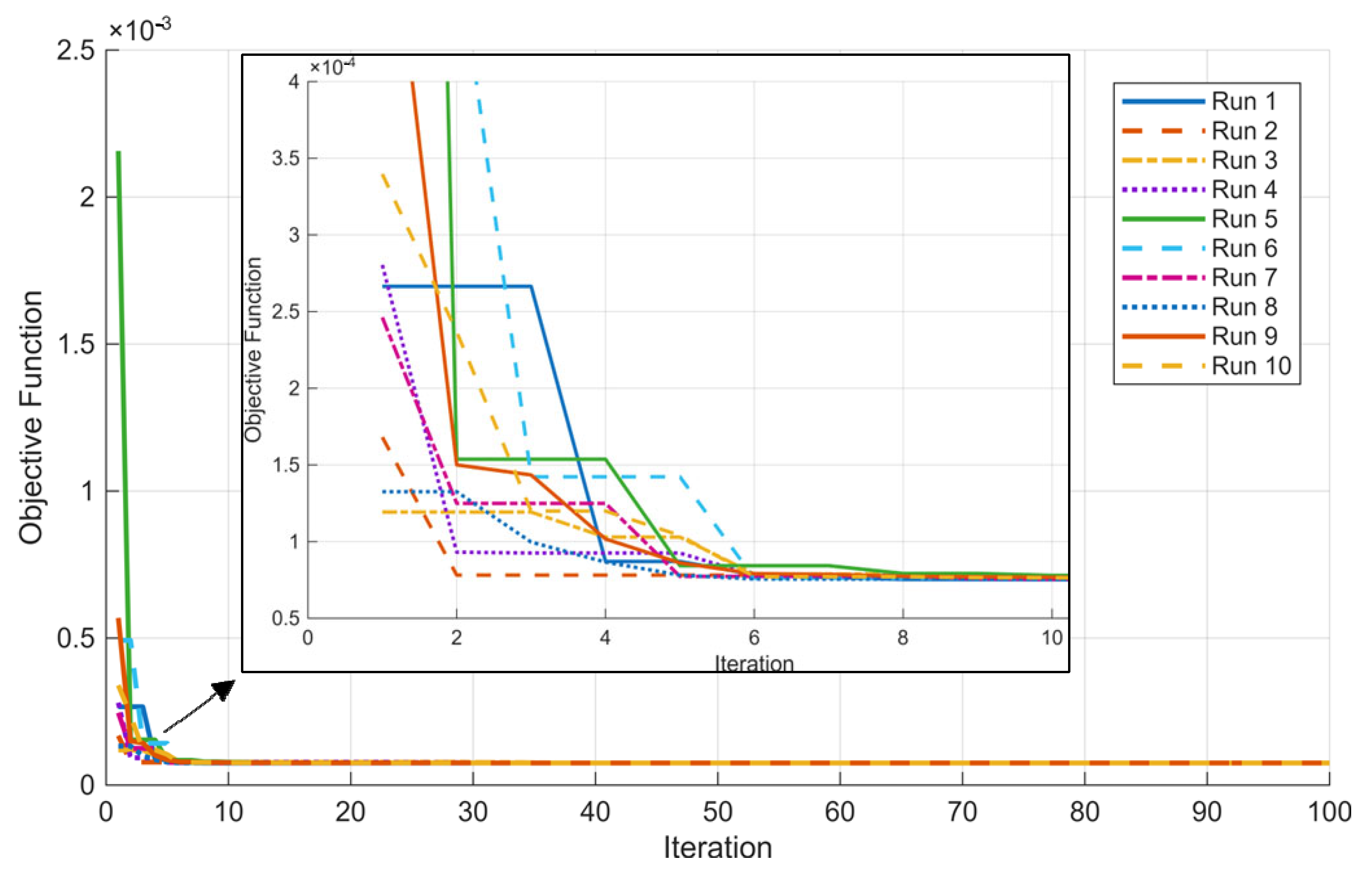
Figure 18 shows changes in the OF over iterations. The largest variance in the OF occurred until the 10th iteration, when we observed different starting values depending on the randomly generated initial population. Smaller variations can be seen up to 30 iterations, whereas some optimization runs needed 40 to 50 iterations to stop changing. The highest OF value was for the fifth run, and the lowest was for the third run.

Figure 18. OF value during optimization for each run.

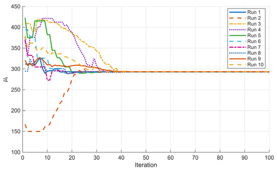
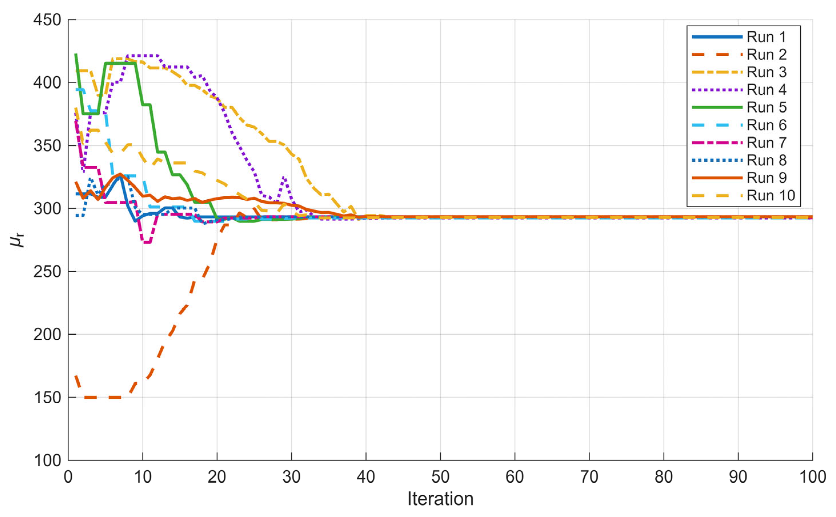
The changes in relative permeability during optimization for each run are presented in Figure 19. Only the second run hits the parameter limit at the lowest limit (Table 5). The fastest run was first, settling after 17 iterations, and the slowest, the second run settled after 43 iterations.

Figure 19. Changes in relative permeability during optimization for each run.

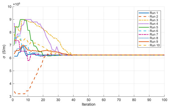
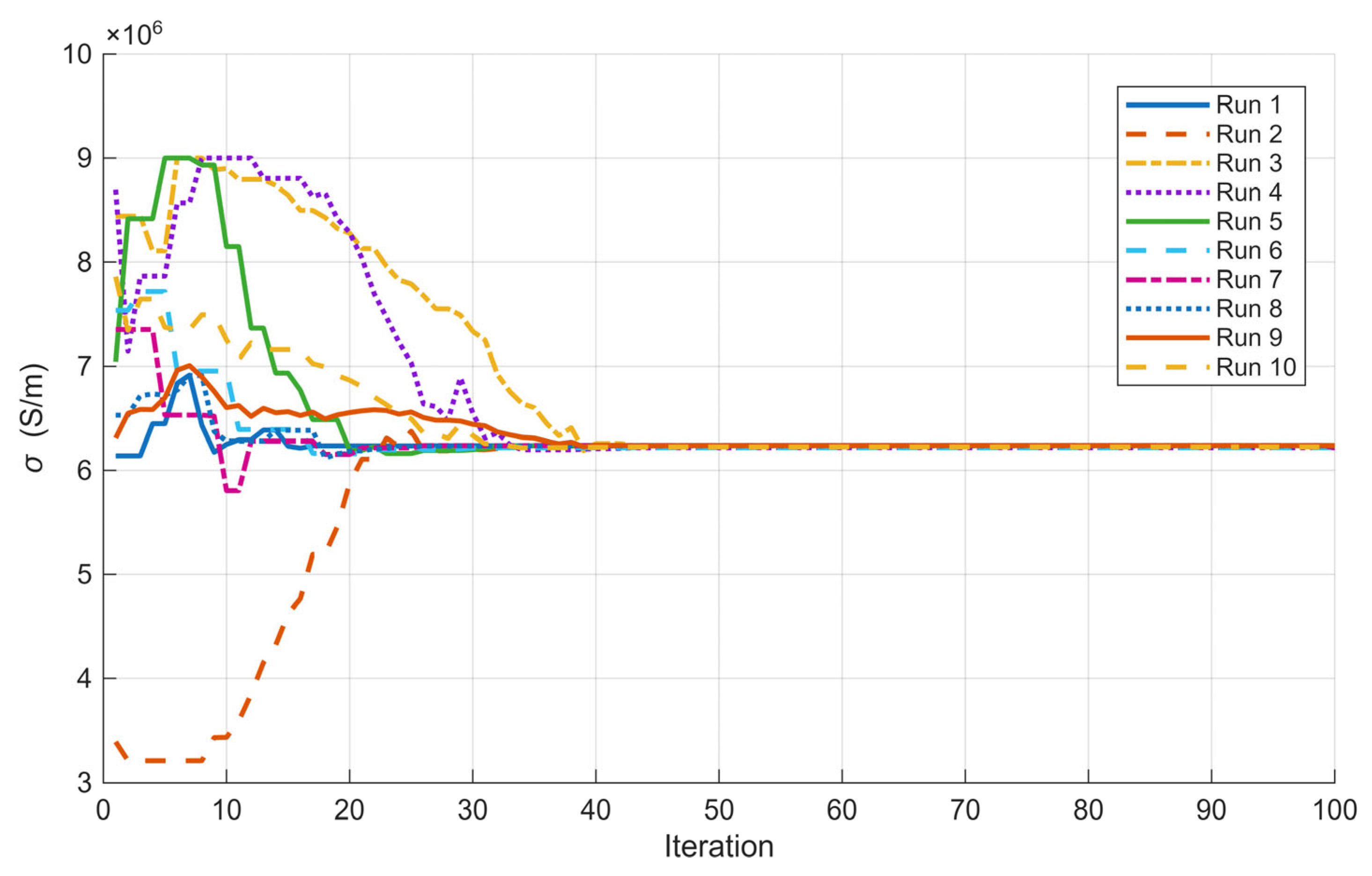
The changes in conductivity during each run’s optimization are shown in Figure 20. There, the second, third, and fifth runs hit the upper limit of the parameters, and none hit the lower limit. The settling of the fastest and slowest parameters was the same as for relative permeability.

Figure 20. Changes in conductivity during each run’s optimization.

In Figure 18, it is evident that the OF experiences a rapid decline and stabilizes in fewer than 10 iterations. In contrast, Figure 19 and Figure 20 show that the desired parameters continue to fluctuate throughout most of the 10 calculations, until approximately 40–50 iterations. Upon examining the variations in relative permeability and conductivity, it becomes apparent that these parameters tend to change in tandem across most of the 10 calculations. When the optimization method generates a new population, both parameters commonly see simultaneous increases or decreases.

5. Brief Overview of the Process

For practical implementation of the presented approach and method, we prepared the following short review in steps for the determination of the conductivity and permeability of the material:

• Step 1: For the measurement of the electrical parameters, we need the following.

A coil and power supply: the coil parameters depend on the power supply we can use. Additionally, the coil needs to be cylindrical. We used a coil with 1112 turns of copper wire, with a diameter of 1.2 mm, an internal diameter of 40 mm, an external diameter of 100 mm, and a length of 46 mm.

The power supply used was an Elgar SW 5250A (Ametek Programmable Power, San Diego, CA, USA).

The measuring instrument can be a true root-mean-square (RMS) multimeter that supports AC measurements up to 600 V. We recommend using an instrument that can measure voltage, current, and power directly, or a power analyzer, as we did. We used the LEM Norma 4000 power analyzer (Fluke Corporation, Everett, WA, USA).

The measured electrical quantities are the basis for determining the material parameters. If there are errors in the measured parameters, they will affect the results. Therefore, electrical parameter measurements must be carried out as carefully as possible.

A steel plate or sample on which we would like to determine the conductivity and permeability is also needed, ideally a little thicker than skin depth and circular, with a diameter larger than the coil’s external diameter. We used a low-carbon circular steel plate with a diameter of 200 mm and a thickness of 1 mm.

The steel plate needs to be placed on the coil, ideally with the centers of each aligned as shown in Figure 2. Wiring connected correctly based on the power instrument and power supply used, with a set frequency of 1000 Hz and the correct supplying values. We measured the voltage, current, and power.

• Step 2: Creation of the FEM model.

For creating the FEM model, the dimensions of the coil and plate used are needed. In our case, the coil had the dimensions listed in Step 1, Section 2.1, and the model was constructed as shown in Figure 4, with the materials listed in Table 1. Depending on the program used, it is important to consider using a skin-depth mesh, as shown in Figure 6, to ensure sufficient mesh layers in that region.

• Step 3: Optimization.

For optimization, we selected a method, coupled it to the FEM model, and performed a search over the plate’s conductivity and permeability. We connected Matlab with Ansys and used DE with the DE/rand/1/exp strategy, which has proven to be robust and reliable.

The presented approach is very flexible and supports the use of different coils, power supplies, and measuring instruments, measuring only electrical parameters, which is more convenient than measuring magnetic parameters. Samples and coils can be different sizes. We recommend using round samples, which allow the creation of a 2D axisymmetric model that has proven to be the most convenient for analysis. Due to the fact that the field ends in the area above the coil, it is important that the plate is larger than the coil.

6. Conclusions

The paper introduced an approach to contactless measurement of relative permeability and conductivity based on measured electrical values and DE optimization. Such an approach can be used to acquire the electromagnetic properties of an unknown low-carbon steel, as in our case, without an expensive, space-consuming installation, using only electrical instruments and an FEM program with optimization.

In Section 2.1, we presented the design and parametrization of the three models used in the first part of the study. The models used were a whole 3D model, a 1/8 symmetrical 3D model, and a 2D model. In the preliminary research runs, we saw the importance of using a skin-depth mesh for our case. We presented an FEM mesh of the 2D Model in Ansys, with particular attention to the mesh in the skin-depth region. We measured the permeability and conductivity of the low-carbon steel plate using laboratory equipment. Then we characterized the coil, both with and without the plate. The results were later used for optimization.

We prepared the model as described in Section 3, using an Ansys Maxwell Circuit to obtain additional parameters for the coil analyzed as a winding. We assumed the plate’s permeability as a scalar value. We defined the reference values used for the optimization and the goal we aimed to reach. The selected optimization method was DE with the DE/rand/1/exp strategy. We set the F and CR values based on prior experience and the number of iterations. Based on the measurements and material properties, we set the lower and upper limits for each optimizing parameter. For the optimization, we established connections with Matlab and Ansys and prepared the flowchart for the optimization algorithm (Figure 12). We proposed OF and determined weight values. We finish the chapter by showing some of the most important calculations and verifications.

The results were presented in Section 4, where we first compared the analysis results and times across the different models. The results were very interesting because they show the importance of the skin mesh in these problems. 3D model analysis without a skin mesh returns a totally irrelevant result, a loss in the plate or solid, as reported in Ansys (Table 7). We considered a 1/8 symmetrical model a good alternative to a 3D model, with much lower analysis time, but that was not the case. Used previously for other 3D-symmetric problem models, such as an alternative to the full 3D model, we obtained comparable results. The 2D model performed well in that scenario, delivering fast, accurate results.

The results from 10 runs showed strong performance, with each run yielding sufficient results and a small SD. That shows strong model conditioning and the right parameter settings for the optimization. The OF reached an M value of 7.513 × 10⁻⁵, which we considered good when compared to the measurements. Based on the results, we can see that the sufficient number of iterations in that case would be 50, but we leave 100 to show that it did not change later. From the results, we can propose, for practical use, determining the optimization parameters by running the optimization three times, and, if the SD is small, treating the resulting values as correct.

In future work, we will focus on implementing the optimization using additional strategies to confirm whether our model is widely applicable and identify its limitations. We will also try introducing additional parameters that can be measured easily in practice. The main goal is to develop an approach for the fast determination of the electromagnetic parameters of steel plates using a contactless method.

References

- Melenk, J.M.; Babuška, J. The partition of unity finite element method: Basic theory and applications. Comput. Methods Appl. Mech. Eng. 1996, 139, 289–314. [Google Scholar] [CrossRef] [Scilit]
- Hansbo, A.; Hansbo, P. A finite element method for the simulation of strong and weak discontinuities in solid mechanics. Comput. Methods Appl. Mech. Eng. 2004, 193, 3523–3540. [Google Scholar] [CrossRef] [Scilit]
- Veček, N.; Mernik, M.; Črepinšek, M. A chess rating system for evolutionary algorithms: A new method for the comparison and ranking of evolutionary algorithms. Inf. Sci. 2014, 277, 656–679. [Google Scholar] [CrossRef] [Scilit]
- Veček, N.; Črepinšek, M.; Mernik, M. On the influence of the number of algorithms, problems, and independent runs in the comparison of evolutionary algorithms. Appl. Soft Comput. 2017, 54, 23–45. [Google Scholar] [CrossRef] [Scilit]
- Mallipeddi, R.; Suganthan, P.N.; Pan, Q.K.; Tasgetiren, M.F. Differential evolution algorithm with ensemble of parameters and mutation strategies. Appl. Soft Comput. 2011, 11, 1679–1696. [Google Scholar] [CrossRef] [Scilit]
- Das, S.; Suganthan, P.N. Differential Evolution: A Survey of the State-of-the-Art. IEEE Trans. Evol. Comput. 2011, 15, 4–31. [Google Scholar] [CrossRef] [Scilit]
- Saruhan, H. Differential evolution and simulated annealing algorithms for mechanical systems design. Eng. Sci. Technol. Int. J. 2014, 17, 131–136. [Google Scholar] [CrossRef] [Scilit]
- Mokan, M.; Sharma, K.; Sharma, H.; Verma, C. Gbest guided differential evolution. In Proceedings of the 9th International Conference on Industrial and Information Systems, Gwalior, India, 15–17 December 2014; IEEE: New York, NY, USA, 2014; pp. 1–6. [Google Scholar]
- Chattopadhyay, S.; Sanyal, S.K.; Chandra, A. Optimization of Control Parameters of Differential Evolution Technique for the Design of FIR Pulse-shaping Filter in QPSK Modulated System. J. Commun. 2011, 6, 558–570. [Google Scholar] [CrossRef] [Scilit]
- He, R.J.; Yang, Z.Y. Differential evolution with adaptive mutation and parameter control using Levy probability distribution. J. Comput. Sci. Technol. 2012, 27, 1035–1055. [Google Scholar] [CrossRef] [Scilit]
- Jesenik, M.; Beković, M.; Hamler, A.; Trlep, M. Analytical modelling of a magnetization curve obtained by the measurements of magnetic materials’ properties using evolutionary algorithms. Appl. Soft Comput. 2017, 52, 387–408. [Google Scholar] [CrossRef] [Scilit]
- Jesenik, M.; Ravber, M.; Trbušić, M. Innovative Approach for the Determination of a DC Motor’s and Drive’s Parameters Using Evolutionary Methods and Different Measured Current and Angular Speed Responses. Mathematics 2024, 12, 42. [Google Scholar] [CrossRef] [Scilit]
- Saad, A.; Engelbrecht, A.P.; Khan, S.A. An Analysis of Differential Evolution Population Size. Appl. Sci. 2024, 14, 9976. [Google Scholar] [CrossRef] [Scilit]
- Wang, X.; Yu, X. Differential Evolution Algorithm with Three Mutation Operators for Global Optimization. Mathematics 2024, 12, 2311. [Google Scholar] [CrossRef] [Scilit]
- Rao, R.V.; Savsani, V.J.; Vakharia, D.P. Teaching-learning-based optimization: A novel method for constrained mechanical design optimization problems. Comput. Aided Des. 2011, 43, 303–315. [Google Scholar] [CrossRef] [Scilit]
- Rao, R.V.; Savsani, V.J.; Vakharia, D.P. Teaching-Learning-Based Optimization: An optimization method for continuous non-linear large scale problems. Inf. Sci. 2012, 183, 1–15. [Google Scholar] [CrossRef] [Scilit]
- Rao, R.V.; Patel, V. An elitist teaching-learning-based optimization algorithm for solving complex constrained optimization problems. Int. J. Ind. Eng. Comput. 2012, 3, 535–560. [Google Scholar] [CrossRef] [Scilit]
- Črepinšek, M.; Liu, S.-H.; Mernik, L. A note on Teaching-learning-based optimization algorithm. Inf. Sci. 2012, 212, 79–93. [Google Scholar] [CrossRef] [Scilit]
- Waghmare, G. Comments on “A note on teaching-learning-based optimization algorithm”. Inf. Sci. 2013, 229, 159–169. [Google Scholar] [CrossRef] [Scilit]
- Deng, W.; Xu, J.; Song, Y.; Zhao, H. Differential evolution algorithm with wavelet basis function and optimal mutation strategy for complex optimization problem. Appl. Soft Comput. J. 2021, 100, 106724. [Google Scholar] [CrossRef] [Scilit]
- Zeng, Z.; Udpa, L.; Udpa, S.S. Finite-Element Model for Simulation of Ferrite-Core Eddy-Current Probe. IEEE Trans. Magn. 2012, 46, 905–909. [Google Scholar] [CrossRef] [Scilit]
- Xiong, L.; Xia, Z.; Huang, R.; Wang, S.; Zheng, X.; Shen, J.; Pang, X.; Yin, W. Through Thickness Inspection of Layered Magnetic Material Using Pulsed Eddy-Current Testing. IEEE Trans. Instrum. Meas. 2023, 72, 6009109. [Google Scholar] [CrossRef] [Scilit]
- Olszewski, E.J.; Cormack, G.D. Contactless measurement of conductivity of metals and semiconductors and of plating thickness of sheet conductors. IEEE Trans. Instrum. Meas. 1976, IM-25, 186–190. [Google Scholar] [CrossRef] [Scilit]
- Yin, W.; Peyton, A.J.; Dickinson, S.J. Simultaneous Measurement of Distance and Thickness of a Thin Metal Plate with an Electromagnetic Sensor Using a Simplified Model. IEEE Trans. Instrum. Meas. 2004, 53, 1335–1338. [Google Scholar] [CrossRef]
- Zheng, X.; Xia, Z.; She, S.; Zou, X.; Yu, K.; Zhang, Z.; Peyton, A.J.; Shen, J.; Yin, W. High-efficiency method for diffusion velocity of eddy current in metallic plates. Measurement 2025, 250, 117046. [Google Scholar] [CrossRef] [Scilit]
- Xia, Z.; Huang, R.; Lu, M.; Yin, W. Thickness and Permeability Estimation of Metallic Plates by Triple-Frequency Eddy-Current Testing with Probe Lift-Off. IEEE Trans. Instrum. Meas. 2024, 73, 6000208. [Google Scholar] [CrossRef] [Scilit]
- Siakavellas, N.J. Two simple models for analytical calculation of eddy currents in thin conducting plates. IEEE Trans. Magn. 1997, 33, 2245–2257. [Google Scholar] [CrossRef] [Scilit]
- Xia, Z.; Huang, R.; Chen, Z.; Yu, K.; Zhang, Z.; Salas-Avila, J.R.; Yin, W. Eddy Current Measurement for Planar Structures. Sensors 2022, 22, 8695. [Google Scholar] [CrossRef] [Scilit]
- Zhu, W.; Yin, W.; Peyton, A.; Ploegaert, H. Modelling and experimental study of an electromagnetic sensor with an H-shaped ferrite core used for monitoring the hot transformation of steel in an industrial environment. NDT E Int. 2011, 44, 547–552. [Google Scholar] [CrossRef] [Scilit]
- He, D.F.; Zhang, K.; Tang, J. A contactless method to measure the electrical conductivity. In Proceedings of the 3rd IEEE International Conference on Control Science and Systems Engineering (ICCSSE), Beijing, China, 17–19 August 2017. [Google Scholar]
- Gencer, N.G.; Tek, M.N. Electrical conductivity imaging via contactless measurements. IEEE Trans. Med. Imaging 1999, 18, 617–627. [Google Scholar] [CrossRef] [Scilit]
- Lu, M.; Xie, Y.; Zhu, W.; Peyton, A.; Yin, W. Determination of the Magnetic Permeability, Electrical Conductivity, and Thickness of Ferrite Metallic Plates Using a Multifrequency Electromagnetic Sensing System. IEEE Trans. Ind. Inform. 2019, 15, 4111–4119. [Google Scholar] [CrossRef] [Scilit]
- Meng, X.; Lu, M.; Yin, W.; Bennecer, A.; Kirk, K.J. Inversion of Lift-Off Distance and Thickness for Nonmagnetic Metal Using Eddy Current Testing. IEEE Trans. Instrum. Meas. 2021, 70, 6003208. [Google Scholar] [CrossRef] [Scilit]
- Yin, W.; Peyton, A.J. Thickness measurement of non-magnetic plates using multifrequency eddy current sensors. NDT E Int. 2007, 40, 43–48. [Google Scholar] [CrossRef] [Scilit]
- Tong, Q.; Hu, L. Optimal Design and Finite Element Simulation of Induction Cooker Magnetic Circuit. In Proceedings of the 3rd Information Technology, Networking, Electronic and Automation Control Conference (ITNEC), Chengdu, China, 15–17 March 2019. [Google Scholar]
- Xia, Z.; Meng, T.; Huang, R.; Fletcher, A.; Shao, Y.; Lu, M.; Peyton, A.; Yin, W. Physics-Guided Deep Learning for Plate Permeability Estimation with Single to Multiple Frequency Transformation of Eddy-Current Testing. IEEE Trans. Ind. Inform. 2024, 20, 6109–6118. [Google Scholar] [CrossRef] [Scilit]
- Naik, S.; Bag, B.; Chandrasekaran, K. A 2D and 3D Analysis on Electromagnetic Parameters of Spoke-shape Interior Permanent Magnet Synchronous Motor Using FEM. Period. Polytech. Electr. Eng. Comput. Sci. 2023, 67, 181–193. [Google Scholar] [CrossRef] [Scilit]
- Khayami, M.; Rassoli, A.; Feizkhah, A. Optimal geometrical selection of skin mesh: Experimental analysis and numerical optimization. Sci. Rep. 2025, 15, 21263. [Google Scholar] [CrossRef] [Scilit] [PubMed]
- Górecki, K.; Detka, K.; Kaczerski, K. The Influence of the Transformer Core Material on the Characteristics of a Full-Bridge DC-DC Converter. Energies 2022, 15, 6160. [Google Scholar] [CrossRef] [Scilit]
- Al-Timimy, A.; Vakil, G.; Degano, M.; Giangrande, P.; Gerada, C.; Galea, M. Considerations on the Effects That Core Material Machining Has on an Electrical Machine’s Performance. IEEE Trans. Energy Convers. 2018, 33, 1154–1163. [Google Scholar] [CrossRef] [Scilit]
- Villacís, S.; Martínez, J.; Riofrío, A.J.; Carrión, D.F.; Orozco, M.A.; Vaca, D. Energy Efficiency Analysis of Different Materials for Cookware Commonly Used in Induction Cookers. Energy Procedia 2015, 75, 925–930. [Google Scholar] [CrossRef] [Scilit]
Disclaimer/Publisher’s Note: The statements, opinions and data contained in all publications are solely those of the individual author(s) and contributor(s) and not of MDPI and/or the editor(s). MDPI and/or the editor(s) disclaim responsibility for any injury to people or property resulting from any ideas, methods, instructions or products referred to in the content. |
© 2026 by the authors. Licensee MDPI, Basel, Switzerland. This article is an open access article distributed under the terms and conditions of the Creative Commons Attribution (CC BY) license.