


Abstract
The Mw 7.8 Gorkha Earthquake of 25 April 2015 triggered over 25,000 landslides across central Nepal, with 4775 events concentrated in Gorkha District alone. Despite substantial advances in landslide susceptibility mapping, existing studies often overlook the compound role of post-seismic rainfall and lack robust spatial validation. To address this gap, we validated an ensemble machine learning framework for co-seismic landslide susceptibility modeling by integrating seismic, geomorphological, hydrological, and anthropogenic variables, including cumulative post-seismic rainfall. Using a balanced dataset of 4775 landslide and non-landslide instances, we evaluated the performance of Logistic Regression (LR), Random Forest (RF), and eXtreme Gradient Boosting (XGBoost) models through spatial cross-validation, SHapley Additive exPlanations (SHAP) explainability, and ablation analysis. The RF model outperformed all others, achieving an accuracy of 87.9% and a Receiver Operating Characteristic (ROC) Area Under the Curve (AUC) value of 0.94, while XGBoost closely followed (AUC = 0.93). Ensemble models collectively classified over 95% of observed landslides into High and Very High susceptibility zones, demonstrating strong spatial reliability. SHAP analysis identified elevation, proximity to fault, peak ground acceleration (PGA), slope, and rainfall as dominant predictors. Notably, the inclusion of post-seismic rainfall substantially improved recall and F1 scores in ablation experiments. Spatial cross-validation revealed the superior generalizability of ensemble models under heterogeneous terrain conditions. The findings underscore the value of integrating post-seismic hydrometeorological factors and spatial validation into susceptibility assessments. We recommend adopting ensemble models, particularly RF, for operational hazard mapping in earthquake-prone mountainous regions. Future research should explore the integration of dynamic rainfall thresholds and physics-informed frameworks to enhance early warning systems and climate resilience.
1. Introduction
Nepal ranks 11th among the seismically most active countries in the world [1]. Most recently, in the history of strong earthquakes in the region, an earthquake of Mw 7.8 struck Barpak Village of Gorkha District in central Nepal at 11:56 local time on 25 April 2015 (often referred to as the 2015 Nepal Earthquake or Gorkha Earthquake). Nepal had not experienced an earthquake of this scale in the last eight decades [2]. The disaster claimed about 9000 people and led to complete and partial collapse of nearly 1.1 million building structures [3]. In about two years after the earthquake, more than 400 aftershocks of Mw 4.0 or greater were recorded, which collectively triggered thousands of landslides in and around the epicentral region.
Co-seismic landslide damage may often surpass the damage caused by an earthquake itself. In fact, the 2015 Gorkha Earthquake exemplified this situation. The ramification of the co-seismic landslides was particularly acute in the areas surrounding Gorkha District, where about 70% of the residential properties were destroyed and a total of 443 people were killed [2].
Landslides on the Nepal Himalayan mountains are particularly devastating because they often have the potential to wipe out entire communities on top of damaging the building structures, social infrastructure, and socio-economic system [4]. Historical earthquake events, such as the 1934 Bihar–Nepal Earthquake and the 1988 Nepal Earthquake, also triggered a large number of landslides, isolating several human settlements and severely damaging the infrastructure [5]. The 2015 earthquake triggered widespread landslides that led to significant structural damage, displacement of a large number of people, and destruction of entire human settlements [6,7]. These events underscore the limitations of conventional methods of landslide susceptibility assessment, which often fail to capture the complex interplay of the contributing factors. These limitations necessitate the use of more robust methods, such as machine learning (ML) and artificial intelligence (AI) techniques, to accurately assess and predict the susceptibility of mountain slopes to earthquake-induced landslides [8].
Landslides on Nepal mountains are particularly influenced by steep topography, young and complex geology, active thrust fault systems, ongoing mountain-building processes, and uncontrolled anthropogenic activities [9,10]. While much of the landslide research focuses on rain-induced landslides, earthquake-induced landslides remain underexplored. Recent studies (e.g., [11,12], etc.) have applied AI and statistical methods for landslide susceptibility analysis because of the ease of handling large datasets and capturing complex, non-linear relationships. These methods can extract meaningful patterns from historical data and are vital for anticipating future landslide occurrences. For instance, Logistic Regression (LR) models were used in the examination of landslide susceptibility by Rasyid et al. [13], while Pyakurel et al. [14] applied the Random Forest (RF) model and Pham et al. [15] employed the eXtreme Gradient Boosting (XGBoost) algorithm. The research carried out by Huang et al. [16], Shrestha et al. [17], and Wang et al. [18] demonstrates the superior performance of ML models compared to traditional statistical or heuristic methods. However, ML models may still struggle when dealing with uncertainties in the predictor variables.
Recent studies have increasingly emphasized the importance of integrating advanced modeling techniques and detailed field investigations to enhance the understanding of landslide mechanisms and susceptibility. For instance, Wen et al. [19] analyzed a medium-sized landslide in Zhenxiong, Yunnan, China, which led to a major disaster, and highlighted how such moderate-scale events can cause significant damage due to complex failure processes and dynamic motion characteristics. Similarly, Wang et al. [18] developed a two-layer stacking ensemble model to assess landslide susceptibility in Jiacha County, demonstrating the improved predictive performance of advanced machine learning approaches over traditional single models. These recent contributions underscore the necessity of combining robust models with contextual geohazard analysis to improve landslide risk assessment.
Although ML models have shown great potential for landslide susceptibility mapping, their effectiveness largely depends on the quality of the input dataset. Since AI models learn from existing data, a reliable and well-curated dataset is essential for training, evaluating, and validating model performance. A critical issue, often overlooked in the literature, is the classification of conditioning factors for earthquake-induced landslides using a broad range of datasets. Moreover, despite the valuable insights offered by Pyakurel et al. [14] and Shrestha et al. [17], research on co-seismic landslides following the 2015 Nepal Earthquake has notable gaps. One key limitation is the inadequate consideration of rainfall influence on post-earthquake slope stability. Rainfall can significantly modify slope hydrology and trigger slope failures even after a long gap from the end of seismic shaking. However, most studies focus only on the immediate effects of an earthquake and ignore the precipitation-led delayed slope response.
In this research work, we adopt a more comprehensive approach by integrating observed rainfall data from not only the month of earthquake occurrence but also the subsequent two months. This enables a better understanding of hydrological ablation dynamics and enhances the predictive power of landslide susceptibility models. Our study introduces a series of methodological innovations aimed at enhancing the accuracy, interpretability, and generalizability of ML models for earthquake-triggered landslide mapping in the Nepal Himalaya. Unlike previous studies, we also conduct a comparative evaluation of LR, RF, and XGBoost models, demonstrating that ensemble learning methods yield higher accuracy and lower false-negative rates. This enables more reliable identification of high-risk areas, which is crucial for informed hazard mitigation.
A novel contribution of this work is the incorporation of observed rainfall ablation data to account for delayed hydrological triggers of the landslides. To reduce spatial autocorrelation and improve model generalization, we implement cluster-based cross-validation and a Leave-One-Cluster-Out (LOCO) approach across distinct geomorphic zones. To further improve model transparency, we apply SHAP (SHapley Additive exPlanations) analysis to determine the relative importance of predictor variables and interpret model behavior. The framework also includes a comprehensive spatial analysis of conditioning factors. Collectively, these innovations address critical methodological limitations and offer a robust, interpretable, and transferable strategy for modeling earthquake-induced landslide susceptibility in tectonically active mountain regions.
2. Materials and Methods
2.1. Study Area
In the aftermath of the 2015 Nepal Earthquake, fourteen out of the seventy-five districts were designated as the most severely affected (crisis-hit) areas, including the epicentral area of Gorkha District [2], which is the study area for this work. As shown in Figure 1, the study area is in the central region of Nepal (84°27′ E–84°58′ E, 27°15′ N–28°45′ N), with an elevation range from 260 m to 8163 m above mean sea level, and covers 3610 square kilometers.
Figure 1.
Location map of the study area (Gorkha District, Nepal) showing the epicenter of the 2015 Gorkha Earthquake (red star), mapped landslide spots, rivers, and district boundaries. The inset map (top-right) illustrates Nepal’s geographic context within South Asia, while the middle-right panel highlights the study area within Nepal.
The annual average precipitation in the study area is approximately 1942 mm, while the temperature fluctuates between 5 °C and 30 °C. The area is characterized by mountainous terrain abundant in natural resources, with the local populace predominantly reliant on agriculture for their livelihood. The area spans from mid-hill mountains to high Himalayan mountains, characterized by rugged terrain with deeply incised gullies. Its delicate topography includes steep to moderate slopes combined with tectonic structures that contribute to higher slope instability.
Geologically, the study area of Gorkha District lies within the Lesser, Higher, and Tibetan Tethys Himalayas. It comprises rocks from the Precambrian to Mesozoic era, including sedimentary, metamorphic, and igneous rocks. Common rock types include phyllites, schists, marbles, quartzites, gneisses, leucogranite, migmatite, sandstone, shale, and limestone [20]. The study area is bisected by the northward-dipping Main Central Thrust (MCT), which serves as the tectonic boundary between the Higher Himalayan Sequence and the Lesser Himalayan Sequence. Historically, the mountainous terrain within the study area has been subjected to a considerable frequency of landslides [9].
2.2. Landslide Inventory
The precise identification of landslide locations is crucial for assessing landslide susceptibility within a specific area. Hence, it is imperative to create a detailed inventory map of co-seismic landslides. In this study, the detection of landslide locations was achieved by combining existing research findings from Roback et al. [7] and the National Disaster Risk Reduction and Management Authority (NDRRMA) [21] along with manual interpretation of images from Google Earth. Earthquake-induced landslides were verified through a comparative analysis of pre- and post-event imagery using Google Earth’s historical timeline feature, as shown in Figure 2. The mapped landslides were then exported to ArcGIS Pro for further processing and spatial analysis.
Figure 2.
Georeferenced Google Earth imagery used for landslide inventory verification: (a) pre-earthquake image with earthquake-induced landslides marked by red polygons and (b) post-earthquake image showing the co-seismic landslides, marked by red polygons and delineated through visual comparison.
The combination of image analysis and field survey efforts resulted in the identification of a total of 4775 co-seismic landslides, ranging in coverage from 28.7 m2 to 308,428 m2, with an average area of 2776 m2. The dataset containing the identified landslides was randomly divided into two subsets: the training dataset of 3820 items (80%) and the model validation dataset of 955 items (20%), as illustrated in Figure 3. Landslide polygons were converted into 4775 point features using ArcGIS Pro, each labeled as ‘1’ to represent a landslide occurrence.
Figure 3.
(a) Earthquake-induced landslide inventory polygon map. (b) Landslide points and random non-landslide points.
To balance the dataset for binary classification, an equal number (n = 4775) of non-landslide points were generated within the same geographic extent and labeled as ‘0’. A buffer-based sampling method was used to ensure that non-landslide points were spatially independent and not influenced by the same geomorphological or triggering conditions. Specifically, a 100 m buffer was created around each landslide point, and non-landslide samples were randomly drawn from outside these buffer zones. Both landslide and non-landslide point data are presented in Figure 3b.
This approach reduced spatial autocorrelation and ensured distinct class separation between landslide and non-landslide samples. All sampled points—both landslide and non-landslide—were validated to fall within the study area boundary and regions with complete and valid conditioning factor data.
2.3. Landslide Conditioning Factors
In this study, a comprehensive set of 14 landslide conditioning factors (LCFs) was compiled from diverse sources and systematically classified into four distinct categories: seismic and geological, topographical, hydrological, and anthropogenic, as detailed in Table 1 and described subsequently. Numerous previous studies, including the works of [22,23,24], have elucidated the critical importance of these LCFs within the context of landslide evaluations, wherein they serve an essential function in the formulation of landslide susceptibility maps. A digital elevation model (DEM) was downloaded from the ASTER Global Digital Elevation Model, accessible through the official NASA website. The DEM resolution is approximately 30 × 30 m, and it offers a precise depiction of the topography. Subsequently, utilizing DEM data, other supplementary topographic contributing factors were converted into raster data to enable a thorough analysis of the region within the ArcGIS Pro environment with Python-assisted model building.
Table 1.
Summary of data used in this research analysis.
2.3.1. Seismic and Geological Factors
Peak ground acceleration (PGA) and the distribution of local faults were considered as critical factors influencing co-seismic landslides, which are typically triggered by intense ground shaking. PGA serves as a quantitative indicator of seismic hazard and shaking intensity. For this study, PGA data associated with the 2015 Gorkha Earthquake were obtained from the USGS ShakeMap database (https://www.usgs.gov/ (accessed on 24 January 2025)). The original PGA values (in units of gravitational acceleration, g) were rasterized to a 30 m spatial resolution to align with the other thematic layers used in the analysis. As illustrated in Figure 4b, the PGA values within the study area ranged from approximately 0.3 g to 0.74 g, with the highest intensities concentrated near the epicenter. These elevated shaking levels likely contributed to the widespread initiation of co-seismic landslides in the region.
Figure 4.
Seismic causative determinants: (a) distance to fault lines and (b) peak ground acceleration (PGA) distribution map.
In addition, slope stability tends to deteriorate near active faults due to structural weakening, leading to increased landslide susceptibility [27]. To capture this, a geological map from the Department of Mines and Geology (DMG) of Nepal was used to digitize the thrust and fault lines. A Euclidean distance map was generated from these faults (Figure 4a) to represent proximity to geological structures.
Furthermore, geology is an indispensable function in determining the spatial distribution of landslides [28]. This is because different lithological units have different physical properties, and they result in dissimilar permeability and strength values of rocks and soils. The influence of geological parameters on landslides has been well documented in numerous studies. For instance, in the context of Nepal, the lithological layers were identified and analyzed through the modification of existing geological maps [20] and the geomorphological data from the geological map produced by the Department of Mines and Geology (DMG), Nepal. The dataset generated from these maps was further classified into 14 lithological units, as depicted in Figure 5, along with the details of each unit and its corresponding formations. Detailed geological descriptions of each geocode used in the analysis are provided in Supplementary Table S1.
Figure 5.
Geological map of the study area with lithological geocodes and their descriptions.
2.3.2. Topographical Factors
The spatial configurations of the topographic features, elevation, slope, aspect, and curvature, were derived from the DEM data, as shown in Figure 6a–d. According to past research, although no direct correlation exists between elevation and landslide frequency, an observable increase in landslide occurrences is found at higher elevations of the study area, where elevation fluctuates from 196 m to 7933 m above mean sea level. Likewise, the slope of a terrain signifies the steepness at each pixel on the surface, which is computed as the first derivative of the DEM data. Within the study area, the slope extends from 0° to 82.77°. Similarly, the aspect refers to the direction in which the slope faces and is a vital factor in landslide susceptibility modeling because it influences solar radiation exposure and weathering processes. Finally, curvature, a measure of directional change of slope in a specific direction, can be used to differentiate between ridges and valleys, based upon which slope is divided into concave, straight, and convex slopes. This information facilitates an understanding of the morphological characteristics of the landscape and can provide insights into potential landslide-prone regions.
Figure 6.
Topographic factors: (a) aspect, (b) curvature, (c) elevation, and (d) slope.
2.3.3. Hydrological Factors
In this study, we consider drainage proximity, the stream power index (SPI), the topographic wetness index (TWI), and rainfall patterns observed in the months following seismic activity as the hydrological factors. During ground-shaking events, slopes composed of saturated or partially saturated soils undergo loss of shear strength, sometimes also behaving akin to liquid. This phenomenon exacerbates the potential for slope instability and subsequent landslides. The topographic wetness index (TWI) is a particularly noteworthy factor employed to quantify the influence of topography on hydrological processes [29]. It provides valuable insights into the distribution and movement of water across a landscape, thereby helping predict areas of potential slope instability. Figure 7a–d present the hydrological layers, and details of the stations and their measurements are listed in Supplementary Table S2.
Figure 7.
Hydrologic factors: (a) drainage proximity, (b) rainfall, (c) stream power index (SPI), and (d) topographic wetness index (TWI).
Despite the critical role of hydrological factors in triggering landslides, many existing studies have overlooked the contribution of precipitation in modeling co-seismic landslide susceptibility. A significant innovation of this study is the incorporation of rainfall data not only from April 2015 (the month of the earthquake) but also from the two subsequent months (May and June 2015), when numerous delayed landslides were reported. Rainfall data were obtained from 10 ground-based meteorological stations managed by the Department of Hydrology and Meteorology (DHM), Nepal. The data were spatially interpolated using the Inverse Distance Weighting (IDW) method to generate continuous rainfall surfaces. This station-based integration offers a more physically realistic representation of post-seismic hydrological conditions, which is crucial for accurate susceptibility modeling.
2.3.4. Anthropogenic Factors
Among anthropogenic influences, proximity to roads plays a significant role in landslide occurrence [30]. Road construction, excavation, and maintenance activities often disturb slope stability and trigger failures [31,32]. The anthropogenic conditioning factors are illustrated in Figure 8a–c.
Figure 8.
Anthropogenic factors: (a) distance to road, (b) LULC, and (c) NDVI.
Additionally, land use and land cover (LULC) changes modify natural surface conditions, altering slope response to external stresses such as rainfall or seismic shaking [33]. For example, deforestation reduces root reinforcement and slope cohesion, increasing landslide vulnerability [34]. To assess these impacts, we used Landsat 8 satellite imagery to derive the Normalized Difference Vegetation Index (NDVI) in ArcGIS Pro, providing a proxy for vegetation cover and slope stability [35]. High NDVI values indicate denser vegetation and generally greater slope stability. Road network data were sourced from the International Centre for Integrated Mountain Development (ICIMOD) (https://www.icimod.org/ (accessed on 25 January 2025)). Multiple buffer zones were generated around road segments to calculate proximity for each point in the study area. The LULC data for the year of the earthquake (2015) were obtained from the Forest Research and Training Centre (FRTC), Nepal. Together, these layers enable a nuanced understanding of human-induced influences on landslide susceptibility.
2.4. Methodology
We evaluated the effectiveness of LR (a statistical analysis technique) and ensemble models (namely, RF and XGBoost) for co-seismic landslide susceptibility modeling. The methodological flow of this study is depicted in Figure 9, while the entire procedural framework can be systematically categorized into three distinct phases as follows.
Figure 9.
Workflow for predicting earthquake-induced landslide susceptibility using ML.
- Data collection: The preliminary phase encompasses the thorough acquisition of landslide inventory data. This compiled dataset is subsequently divided into two subsets: one designated for model training and the other for result validation. This initial phase entails the collection of diverse data types, including digital elevation models (DEMs), precipitation, slope, aspect, curvature, proximity to fault lines, road networks, water streams, elevation, geological features, land use/land cover (LULC), Normalized Difference Vegetation Index (NDVI), peak ground acceleration (PGA), stream power index (SPI), topographic wetness index (TWI), and earthquake-induced landslide inventory data. These datasets are processed to derive landslide conditioning factors (LCFs) utilizing ArcGIS pro and the Python (Ver. 3.11.11) programming environment.
- Model application: The subsequent phase involves the aggregation of landslide causative factors (CFs). These factors are thereafter subjected to analysis through three widely recognized supervised ML models: RF, LR, and XGBoost. The analytical process is conducted using the training dataset. The data are partitioned into a training set (80%) and a testing set (20%). The algorithms undergo training with the training set to discern the most significant factors via feature importance analysis.
- Result validation and prediction: The final phase involves accuracy assessments of the models using performance metrics like the performance evaluation matrix and Area Under the Curve (AUC) values. The results from the ML models are combined to generate a co-seismic landslide susceptibility map.
2.5. Machine Learning Algorithms
The scikit-learn Python [36] (https://scikit-learn.org (accessed on 25 January 2025)) was employed to implement a variety of ML algorithms in this study. These include LR, RF, and XGBoost. These algorithms were chosen on the basis of a preliminary performance evaluation of algorithms. Below is an enhanced and modified introduction to these algorithms.
2.5.1. Logistic Regression (LR)
Logistic Regression is a statistical model that applies a logistic function to represent a binary dependent variable, making it suitable for binary classification tasks [37]. It is a type of generalized linear model (GLM) used for predicting the probability of a categorically dependent variable. The LR framework is predicated on the logistic function, which manifests an S-shaped curve capable of mapping any real-valued input to a value within the range of 0 to 1. The logistic function is defined as follows [38].
Within the context of LR, the log odds (the logarithm of the odds) corresponding to the outcome labeled “1” is expressed as a linear combination of one or more independent variables (“predictors”). The mathematical representation of the model is articulated as follows.
where p is the probability of the positive class, X is the input (or feature), and β values are the parameters of the model, which are learned from the data.
2.5.2. Random Forest (RF)
The RF methodology represents a sophisticated approach to tree-based learning, entailing the generation of a multitude of decision trees during the training phase. These trees are constructed utilizing random subsets of the dataset, which facilitates the evaluation of a random selection of features within each segment [39]. This inherent randomness fosters diversity among the individual trees, subsequently reducing the likelihood of overfitting and augmenting the overall predictive efficacy. In the prediction phase, the RF algorithm integrates the results from all trees, either through a voting mechanism (for classification tasks) or through averaging (for regression tasks). This collaborative process of decision making, bolstered by the insights derived from multiple trees, culminates in stable and precise outcomes [40]. RFa are extensively employed in both classification and regression applications due to their proficiency in addressing complex data structures, mitigating overfitting, and providing reliable predictions across diverse contexts [12].
2.5.3. eXtreme Gradient Boosting (XGBoost)
XGBoost represents a highly effective ML algorithm, distinguished by its efficiency, rapidity, and precision [38]. It is categorized within the family of boosting algorithms, which are ensemble learning methodologies that amalgamate the predictions of several weak learners. XGBoost constructs a predictive model by iteratively combining the predictions of multiple individual models, frequently decision trees, in a systematic manner [41]. This boosting mechanism is employed to develop an extraordinarily accurate ensemble model, wherein each weak learner rectifies the errors made by its antecedents.
2.6. Multicollinearity Assessment of Predictor Variables
2.6.1. Pearson Correlation Matrix
The Pearson correlation matrix constitutes a tabular representation that delineates the correlation coefficients among various sets of variables. Each coefficient spans a range from −1 to 1, signifying the strength and direction of the linear association between two variables. The correlation coefficient elucidates the degree of relationship between two variables, where +1 denotes a perfect positive correlation, 0 signifies no correlation, and −1 indicates a perfect negative correlation [38]. The matrix shown in Figure 10 illustrates that the input variables designated for training ML models are devoid of multicollinearity.
Figure 10.
Pearson correlation matrix.
2.6.2. Variance Inflation Factor (VIF) and Tolerance Analysis
To assess multicollinearity among the 14 landslide conditioning factors used in the machine learning models, we conducted a Variance Inflation Factor (VIF) and Tolerance analysis. While Pearson correlation assesses linear pairwise relationships, VIF and Tolerance provide a more comprehensive evaluation of inter-variable redundancy in multivariate contexts. VIF quantifies the extent to which the variance of a regression coefficient is inflated due to multicollinearity, with values above 10 typically indicating problematic collinearity. Tolerance, defined as the inverse of VIF, provides a complementary measure of variable independence; values below 0.1 are generally considered concerning.
As summarized in Table 2, all predictor variables had VIF values below the critical threshold of 10 and Tolerance values above 0.1, suggesting that multicollinearity does not pose a serious concern in this study. The highest VIF was observed for distance to fault (7.787), followed by elevation (5.618) and peak ground acceleration (PGA) (4.937). These moderate values likely reflect the shared geophysical characteristics of terrain and seismic proximity. In contrast, most topographic and environmental variables, including slope, TWI, SPI, NDVI, LULC, and aspect, exhibited VIFs close to or below 2, indicating low collinearity and strong statistical independence. The combined use of VIF and Tolerance not only verifies the robustness of our feature set but also ensures that redundant predictors do not undermine the reliability of model interpretation or predictive stability.
Table 2.
Variance Inflation Factor (VIF) and Tolerance values used to assess multicollinearity among predictor variables.
3. Results and Discussion
3.1. Spatial Relationship Between Landslide Distribution and Conditioning Factors
To understand the controlling mechanisms of co-seismic landslides triggered by the 2015 Gorkha Earthquake, we investigated the spatial distribution of landslide area, areal density, and number density across ten key landslide conditioning factors (LCFs). These factors include terrain morphology, seismic input, geological settings, hydrological conditions, vegetation cover, and anthropogenic influences. The spatial distribution maps are presented in Figure 11a–j, illustrating the spatial relationships between landslide metrics and key conditioning factors. Each subplot illustrates three metrics: total landslide area (gray bars), areal density (%) (gold line), and number density (1/km2) (red line), across different classes of conditioning factors.
Figure 11.
Spatial distribution of landslide area (gray bars), areal density (%) (gold lines), and number density (1/km2) (red lines) across classes of (a) aspect, (b) curvature, (c) geology, (d) distance to road, (e) distance to fault, (f) distance to stream, (g) elevation, (h) NDVI, (i) PGA, and (j) slope.
Landslides predominantly occurred on slopes ranging between 30° and 50°, with the highest number density observed in the 40–50° class (Figure 11j). This range appears to represent a critical slope threshold where gravitational stresses most effectively exceed the resisting forces. The areal density similarly peaked in the 50–60° range, indicating that not only were more landslides initiated on moderately steep terrain, but that they also tended to cover larger areas. In contrast, landslide occurrence notably decreased in the steepest slope class (>60°), likely due to the presence of exposed bedrock.
Landslide frequency and area display a pronounced directional pattern, with south-facing (S) and southeast-facing (SE) slopes experiencing the highest number density (up to ~2.0/km2) and areal coverage (around 2.5 km2), as in Figure 11a. These aspects are typically exposed to higher solar radiation, which may induce surface desiccation, reduce vegetation density, and lead to diminished root cohesion, collectively weakening slope stability. In contrast, north- and northwest-facing slopes, as well as flat terrain, exhibit relatively lower landslide densities and areas, possibly due to denser vegetation, more stable moisture retention, or reduced weathering intensity.
Landslides occurred predominantly on concave (negative-curvature) slopes, which showed the highest landslide area and number density, as in Figure 11b. These landforms tend to accumulate water, increasing pore pressure and promoting failure. In contrast, flat surfaces exhibited minimal landslide activity, while convex slopes showed moderate susceptibility, likely due to their tendency to shed water and reduce subsurface saturation. Landslides were predominantly concentrated in three key geological formations: the Ghan Pokhara Formation (Gp), the Ranimatta Formation (Rm), and the Higher Himalayan Crystalline (Hm), as in Figure 11c. The Gp unit, rich in carbonaceous slates and shales, showed the highest landslide number density, reflecting its weak and weathered lithology. The Rm unit, composed of phyllites and quartzites with intrusions, exhibited moderate susceptibility due to structural complexity. The Hm unit, though relatively stronger, still recorded notable landslides, likely along foliated zones within its gneisses and schists.
Anthropogenic influences were evident. Over 50% of the total landslide area occurred within 0–1000 m from roads, with both areal and number density showing steep declines beyond 1000 m. This reinforces the destabilizing impact of slope undercutting, improper drainage, and toe removal during road construction in steep terrains. More than 50% of mapped landslides were within 0–3000 m of active faults. The number density was especially elevated in the 0–2000 m range, underscoring the direct influence of strong ground motion amplification and tectonic fracturing near fault zones. A large proportion of landslides were observed within 0–1000 m of streams. High areal densities were evident in the 250–500 m range, suggesting that incision, groundwater accumulation, and undercutting along fluvial corridors play a crucial role in slope destabilization. Mid-elevation belts between 1000 and 2000 m recorded the highest landslide concentrations. Landslides showed higher densities in areas with NDVIs between 0.2 and 0.5. These values reflect moderately vegetated slopes where root cohesion may be insufficient to stabilize disturbed soils during strong shaking. Densely forested zones (NDVIs > 0.6) exhibited a lower landslide frequency, indicating a protective effect of vegetation.
The highest number and density of landslides occurred within the 0.6–0.7 g range, particularly in areas closer to the epicenter. This aligns with zones of intense seismic shaking, confirming PGA as one of the most influential triggers in the study region. Together, these findings highlight the spatially conditioned nature of co-seismic landslides, where the interplay of seismic forces with terrain, lithology, hydrology, and human activities determines the likelihood of failure. The results are consistent with past studies [42,43] and reinforce the need for multifactorial susceptibility modeling.
3.2. Confusion Matrix Evaluation
A confusion matrix serves as a comprehensive framework to evaluate the performance of a classification model against a labeled test dataset. It reports the number of correct and incorrect predictions, categorized as true positives (TPs), false negatives (FNs), false positives (FPs), and true negatives (TNs), and provides insight into the strengths and weaknesses of model performance [38]. This tool is particularly valuable in assessing how well a model performs across different classes, especially in binary classification problems such as landslide vs. non-landslide classification. The classification reports and visual confusion matrices for the selected models (RF, LR, and XGBoost) are presented in Figure 12, while their numerical values and derived metrics are summarized in Table 3.
Figure 12.
Classification report and confusion matrix for models: (a) RF, (b) LR, and (c) XGBoost.
Table 3.
Confusion matrix elements and derived metrics for the RF, LG, and XGBoost models.
To provide a more comprehensive assessment beyond global metrics such as accuracy and AUC, we conducted an in-depth evaluation of confusion matrix-derived indicators. Among the models, the Random Forest classifier demonstrated the highest recall of 90.91%, corresponding to the lowest false-negative rate (FNR) of 9.09%, indicating superior sensitivity to actual landslide occurrences. XGBoost achieved a comparable recall of 89.58% with an FNR of 10.42%, also showing strong capability in detecting hazard-prone zones. In contrast, LR exhibited a lower recall of 82.64% and a higher FNR of 17.36%, suggesting a greater risk of underreporting landslide-susceptible areas. These findings emphasize the importance of incorporating class-specific metrics, particularly recall and FNR, into model evaluation protocols, as relying solely on aggregate measures may obscure critical performance deficiencies. In the context of landslide susceptibility mapping, minimizing false negatives is particularly important, as undetected high-risk zones can lead to severe socio-economic and infrastructural consequences
3.3. Model Performance Parameters
Model performance parameters are metrics that are extrapolated from the confusion matrix, providing a nuanced understanding of the model performance. Below are some key parameters computed using Python on the test data [38].
Accuracy: This metric represents the ratio of the total number of correct instances to the total number of instances. It can be calculated as follows.
Precision: This metric signifies the ratio of correctly predicted positive observations to the total number of predicted positives. It is calculated as follows.
Recall (Sensitivity): This metric represents the proportion of accurately identified positive instances relative to the total number of instances within the actual classification. It is computed as follows.
Matthews Correlation Coefficient (MCC): The MCC serves as a more robust statistical measure that yields elevated scores exclusively when the predictive model demonstrates efficacy across all four categories within the confusion matrix (true positives, false negatives, true negatives, and false positives), while concurrently taking into account the proportionality of both positive and negative instances within the dataset. It functions as an indicator of the performance quality of binary classifiers. This metric integrates both true and false positives, as well as true and false negatives, and is widely acknowledged as a balanced metric applicable even in scenarios where the sizes of the classes diverge significantly. The MCC fundamentally represents a correlation coefficient that ranges from −1 to +1. A value of +1 denotes a flawless prediction, while 0 indicates a prediction equivalent to random chance and −1 signifies an inverse prediction. The formula for the MCC is articulated as follows.
where TP = true positives, TN = true negatives, FP = false positives, and FN = false negatives.
Cohen’s Kappa: Cohen’s Kappa is a statistical measure employed to assess inter-rater reliability (as well as intra-rater reliability) concerning qualitative (categorical) items. It is typically regarded as a more resilient measure in comparison to a straightforward percentage agreement calculation, given that κ incorporates the potential for agreement arising due to chance. Nevertheless, it is important to acknowledge the ongoing discourse surrounding the application of Cohen’s Kappa, attributable to its relative nature, which complicates the interpretation of its resultant values. The formula for Cohen’s Kappa is as follows.
where po is the relative observed agreement among raters (identical to accuracy) and pe is the hypothetical probability of chance agreement.
To evaluate the predictive performance of the models RF, XGBoost, and LR, we computed a comprehensive set of classification metrics beyond overall accuracy. These included precision, recall, specificity, F1 score, Matthews Correlation Coefficient (MCC), and Cohen’s Kappa, as summarized in Table 4. Among the models, Random Forest achieved the highest overall performance, with a recall of 0.909 and an F1 score of 0.885, followed closely by XGBoost. Although Logistic Regression had slightly lower performance, it remains interpretable and helpful in understanding the influence of each variable.
Table 4.
Classification performance metrics for models.
Notably, recall plays a critical role in landslide susceptibility mapping. It quantifies the model’s ability to identify actual landslide occurrences (true positives) correctly. In the context of disaster risk management, high recall is essential to minimize false negatives, that is, locations prone to landslides being misclassified as safe. Such errors could lead to serious safety and infrastructure consequences. Hence, the high recall values obtained by the ensemble models (especially RF and XGBoost) underline their suitability for landslide prediction tasks. This comprehensive metric evaluation ensures robust and balanced interpretation of the models’ classification capabilities, with an emphasis on minimizing the risk of overlooking hazardous zones.
3.4. Statistical Comparison of Model Performance
To determine whether the observed performance difference between RF and XGBoost was statistically significant, we conducted a series of comparative analyses. Although both models achieved similarly high AUC scores (RF = 0.94; XGBoost = 0.93), DeLong’s test [44] revealed a statistically significant difference in their ROC curves (Z = −2.20, p = 0.0278), indicating that RF more consistently ranked positive instances higher than XGBoost across the test set. These results suggest that even subtle differences in AUC can have meaningful implications for the reliability of landslide prediction.
To assess whether the RF and XGBoost models differ significantly in their classification patterns, the McNemar test [45] was applied to the distribution of discordant predictions. Among 111 discordant pairs, RF correctly classified 59 instances that XGBoost misclassified, while XGBoost correctly classified 52 instances that RF misclassified. The resulting McNemar test statistic was χ2 = 0.441, yielding a p-value of approximately 0.507. This indicates no statistically significant difference in the error patterns of the two models (p > 0.05). An exact binomial test, based on the assumption of equally likely discordant outcomes, confirmed this result. These findings suggest that while RF and XGBoost differ slightly in metrics such as AUC and area-based susceptibility zoning, their classification errors are statistically equivalent. Therefore, model selection may be better guided by factors such as interpretability, spatial generalization, or practical mapping outcomes rather than marginal differences in predictive performance.
Compared to previous studies such as Pyakurel et al. [14], which reported 85.7% accuracy and 0.89 AUC using RF, our model achieved improved performance (accuracy = 87.9%; AUC = 0.94 under standard and 0.89 under spatial cross-validation). These gains are attributed to the incorporation of post-seismic rainfall, spatial cross-validation, and advanced tuning. Overall, RF slightly outperformed XGBoost, but both are robust models for co-seismic landslide susceptibility modeling in mountainous terrain.
3.5. Model Validation Using ROC Curve
The receiver operating characteristic (ROC) curve was employed to assess the performance of the landslide susceptibility maps obtained from the three ML models. The ROC curve is a critical tool for comparing the sensitivity and specificity of binary classification models, thereby facilitating the selection of the most suitable model based on the trade-off between the true-positive rate (TPR) and the false-positive rate (FPR).
3.5.1. Cross-Validation Using Coordinate-Based Approach
To evaluate model robustness under spatial heterogeneity, we employed a 10-fold cross-validation strategy based on X and Y coordinates, rather than relying on conventional random K-fold approaches. The dataset used in this approach was well-balanced between landslide and non-landslide classes. This balance helped prevent bias during model training and contributed to the stable and accurate performance observed across all folds.
We evaluated the performance of three machine learning classifiers: LR, RF, and XGBoost. As shown in Figure 13, the RF and XGBoost models outperformed LR in terms of both average AUC and consistency across folds. The mean AUC values achieved were 0.944 for RF, 0.940 for XGBoost, and 0.875 for LR. This demonstrates the superior ability of ensemble tree-based models to capture the complex, non-linear relationships inherent in landslide processes and their robustness in capturing complex and non-linear landslide-triggering mechanisms under spatially heterogeneous conditions. While LR still maintained a relatively high performance, its lower average AUC and greater variability suggest a reduced ability to generalize in the presence of spatial heterogeneity. These findings highlight the importance of adopting cross-validation strategies that account for geographic autocorrelation. Unlike traditional random K-fold methods, coordinate-based partitioning ensures that model performance reflects real-world deployment scenarios. The consistent superiority of RF and XGBoost in this setting validates their application for operational landslide susceptibility mapping in mountainous and spatially complex regions such as the central Nepal Himalayas.
Figure 13.
ROC curves for 10-fold cross-validation using X and Y coordinate-based random partitioning. The colored lines represent the average ROC for each model, the shaded lines show individual fold performance, and the dashed inclined line indicates an AUC value of 0.5. The embedded boxplot displays the AUC score distribution across folds.
3.5.2. Model Performance Across Spatial Clusters
To evaluate spatial generalizability, we applied a Leave-One-Cluster-Out (LOCO) cross-validation scheme by dividing the study area into three distinct clusters (1, 2, and 3), as shown in Figure 14a. Each cluster served as an independent test fold, while the remaining two were used for training. This spatially independent validation simulated realistic deployment scenarios, where predictions had to be made in previously unseen and geologically distinct regions. The performance of three classifiers, LR, RF, and XGBoost, was evaluated using two key metrics: the Area Under the Receiver Operating Characteristic Curve (ROC AUC) and the Area Under the Precision–Recall Curve (PR AUC). The results are summarized in Supplementary Table S3, while fold-wise and mean ROC curves are presented in Figure 14b.
Figure 14.
(a) Spatial clusters used for Leave-One-Cluster-Out (LOCO) cross-validation within the study area. (b) ROC curves illustrating fold-wise and mean AUC performance of models under the LOCO scheme. Bold lines represent mean ROC curves across folds while the dashed inclined line indicates an AUC value of 0.5.
In Fold 1, LR exhibited the weakest performance (ROC AUC = 0.670, PR AUC = 0.735), highlighting its limitations in capturing non-linear spatial patterns. In contrast, RF and XGBoost performed substantially better, with RF achieving an ROC AUC of 0.833 and a PR AUC of 0.864 and XGBoost reaching an ROC AUC of 0.804 and a PR AUC of 0.851. For Fold 2, all models improved. LR achieved an RO AUC = 0.869, while RF and XGBoost reached ROC AUC values of 0.920 and 0.926, respectively. Their PRAUC scores (RF = 0.900, XGBoost = 0.905) also underscore their superiority in predicting landslide-prone zones. In Fold 3, all models maintained relatively high performance. LR recorded an ROC AUC = 0.892 and a PR AUC = 0.836, while RF and XGBoost showed consistent accuracy with ROC AUCs of 0.906 and 0.905 and PR AUCs of 0.863 and 0.857, respectively.
These results (Figure 14) demonstrate that tree-based models consistently outperform LR, especially under spatially independent conditions. The LOCO framework effectively highlights model robustness and minimizes the risks of overfitting due to spatial autocorrelation, making RF and XGBoost reliable tools for operational landslide susceptibility mapping. Overall, the results indicate that tree-based ensemble models (RF and XGBoost) consistently outperform linear classifiers, such as LR, across spatially distinct regions. These findings highlight the advantage of non-linear, ensemble learning methods in capturing complex spatial interactions among landslide conditioning factors. Moreover, the Leave-One-Cluster-Out spatial cross-validation approach emphasizes the importance of accounting for geographic heterogeneity during model training and validation. It mitigates the risk of spatial leakage and overfitting, which are common in random cross-validation settings, and thus provides a more realistic and conservative estimate of model performance for spatial landslide susceptibility prediction.
3.6. Ablation Experiment: Contribution of Rainfall Factor
To assess the specific contribution of post-seismic rainfall in co-seismic landslide susceptibility modeling, an ablation study was performed. The rainfall predictor, primarily based on cumulative rainfall for April to June 2015, was removed from the dataset, and the RF, XGBoost, and LR models were retrained using the reduced feature set. The performance of the modified models was then systematically compared with their full-feature counterparts to quantify the predictive value of rainfall in landslide triggering under post-seismic conditions.
The results (Table 5) show that the exclusion of the rainfall feature led to a noticeable decline in all evaluation metrics, particularly ROC AUC, recall, and F1 score, across all models. This decline confirms that rainfall, despite being a secondary triggering factor following seismic activity, plays a substantial role in the physical processes underlying landslide initiation. Specifically, RF’s AUC dropped from 0.94 to 0.93, while its recall decreased from 0.909 to 0.881, highlighting a reduced capacity to detect true-positive landslide events in the absence of hydrological data.
Table 5.
Model performance with and without rainfall features.
Introducing rainfall into the model not only improved sensitivity but also enhanced model balance, as indicated by elevated F1 scores. RF achieved the best performance among all models with rainfall features, attaining an accuracy of 0.879, a recall of 0.909, and an F1 score of 0.885. XGBoost also experienced performance gains, particularly in precision and F1 score, underscoring the value of rainfall as a contributing factor in ensemble learning models. While Logistic Regression remained the lowest performant of the three, it too benefited from rainfall input, with notable gains in accuracy, recall, and ROC AUC.
Figure 15 provides a comparative visual summary of model behavior through a radar chart illustrating five core metrics: accuracy, precision, recall, F1 score, and ROC AUC. The inclusion of rainfall predictors results in a visibly broader radar footprint, particularly for RF and XGBoost models, reflecting more balanced and improved performance across all metrics. The RF model demonstrates the most consistent and superior performance, followed closely by XGBoost. Even LR, though conservative in its predictions, shows measurable improvement, reinforcing the hydrological relevance of rainfall in post-seismic slope stability.
Figure 15.
Model performance comparison with and without rainfall.
These findings support the incorporation of hydro-meteorological variables into susceptibility models, particularly in earthquake-prone regions where precipitation can act as a secondary but powerful landslide trigger. The enhancement of classification performance upon the inclusion of rainfall data supports the hypothesis that rainfall, especially in the months immediately following a seismic event, makes a significant contribution to the geotechnical destabilization of slopes.
3.7. Feature Contribution Analysis Using SHAP Values
To better understand the non-linear interactions between key landslide conditioning factors, SHAP (SHapley Additive exPlanations) interaction plots were generated. SHAP is a game-theoretic approach that assigns each feature an importance value for a particular prediction. The SHAP value quantifies the impact of an individual feature on the model’s output: positive SHAP values indicate an increase in the predicted probability of landslide occurrence, while negative values suggest a decrease. In the graphical outputs, features are plotted along the Y-axis, and their SHAP values are shown on the X-axis. The color gradient represents feature values, with blue indicating lower values and red indicating higher values.
The SHAP beeswarm summary plot (Figure 16a) and mean SHAP value plot (Figure 16b) reveal the relative importance and directional influence of landslide conditioning factors. Among all features, elevation exhibited the highest mean SHAP value (+1.55), indicating its dominant role in increasing landslide susceptibility, particularly in high-altitude zones. Other prominent features included distance to fault (+0.92), peak ground acceleration (PGA) (+0.78), slope (+0.68), and distance to stream (+0.64). These results underscore the significant contribution of topographic and seismic factors in co-seismic landslide initiation.
Figure 16.
SHAP analysis. (a) Beeswarm plot showing feature impacts on landslide prediction. (b) Bar chart of mean SHAP values.
The beeswarm plot further illustrates how high values of elevation, slope steepness, and ground acceleration contribute positively to landslide probability, as indicated by the clustering of red-colored points with high SHAP values. In contrast, features such as NDVI, distance to road, and aspect showed lower SHAP values, reflecting more modest but still relevant roles in the predictive framework. Notably, the distance to stream displayed both positive and negative SHAP values across its range, indicating a non-linear relationship with landslide susceptibility. This highlights the advantage of SHAP in capturing complex feature interactions that are often overlooked by traditional linear feature importance metrics. The distance to fault and PGA reveal heightened feature importance, which are pivotal conditioning factors for the co-seismic landslides.
Further insights into feature interdependencies were obtained through SHAP interaction plots (Figure 17). The elevation × distance to fault interaction (Figure 17a) revealed that landslide probability was highest at elevated terrains in close proximity to fault lines. This spatial combination likely reflects the presence of structurally weakened lithologies and fractured bedrock in tectonically active zones. Similarly, the PGA × slope interaction (Figure 17b) indicated that steep slopes subjected to high seismic acceleration showed markedly elevated susceptibility. These compound effects suggest that ground shaking and steep terrain amplify landslide hazards synergistically, affirming the geomechanical relevance of multi-variable interactions in co-seismic settings.
Figure 17.
SHAP interaction plots illustrating the compound effects of (a) elevation × distance to fault and (b) peak ground acceleration (PGA) × slope on landslide susceptibility predictions.
Overall, the SHAP-based analysis enhances both the interpretability and geoscientific robustness of the machine learning models. By elucidating how different factors, both alone and in interaction, contribute to landslide probability, this approach supports more transparent and informed susceptibility mapping. It also emphasizes the importance of considering complex, non-linear relationships when modeling natural hazard phenomena, such as earthquake-induced landslides.
3.8. Landslide Susceptibility Mapping and Comparison of Models
Figure 18 presents the earthquake-induced landslide susceptibility maps generated using LR, RF, and XGBoost models. The continuous probability outputs from each model were classified into five susceptibility zones: Very Low, Low, Medium, High, and Very High, using the Jenks natural breaks algorithm to ensure optimal class separation. A comparative spatial analysis reveals that RF and XGB yield highly consistent susceptibility patterns, delineating concentrated zones of High and Very High risk, particularly along steep terrain and fault-aligned valleys. These zones are prominently clustered near the earthquake epicenter and the active faults, underscoring the dominant role of seismic ground motion and structural discontinuities in the occurrence of landslides. In contrast, the LR model produces more generalized and spatially diffused susceptibility patterns, reflecting the limitations of linear modeling in capturing complex terrain interactions. Nevertheless, all three models consistently identify central and southeastern sectors of the study area as prone to landslides.
Figure 18.
Earthquake-induced landslide susceptibility maps developed by (a) LR model, (b) RF model, and (c) XGBoost model.
3.8.1. Area Distribution of Susceptibility Classes
Figure 19 compares the spatial distribution of landslide susceptibility zones across the five classification levels for the three models. Each model displays distinct patterns that reflect their internal decision-making processes. The LR model assigned 46.56% of the study area to the Very Low class and only 5.13% to the Very High class, indicating a conservative estimation approach with broader allocation to lower-risk zones. The RF model, while more refined, allocated 65.94% to the Very Low class and 4.24% to the Very High class, reflecting a slightly more balanced but still cautious delineation. In contrast, XGBoost displayed the most aggressive zoning behavior, allocating 75.87% of the area to the Very Low class and 7.69% to the Very High class, with notably narrow assignments to the Low (6.84%) and Medium (4.88%) categories. This pattern indicates heightened model sensitivity to terrain and seismic variability.
Figure 19.
Comparison of landslide susceptibility classes across three predictive models. Colored horizontal bars represent the total area (km2) in each susceptibility class, while dashed lines with markers denote the corresponding percentage of the study area.
Despite the relatively small proportion of areas falling within High and Very High zones (ranging from 9.37% in RF to 12.4% in XGBoost), these zones spatially coincide with observed landslide clusters, particularly near fault lines and the epicenter. This spatial alignment affirms the credibility of the models in identifying geologically unstable regions. Overall, the comparative area distributions suggest that LR is conservative, RF strikes a balance between caution and specificity, and XGBoost maximizes detection sensitivity by capturing complex geomorphological patterns.
3.8.2. Landslide Count-Based Verification of Susceptibility Classes
Figure 20 presents the spatial distribution of observed landslides across susceptibility classes predicted by the LR, RF, and XGBoost models. Ensemble models, particularly RF and XGBoost, exhibited high classification accuracy, with 98.0% and 95.7% of landslides located in the combined High and Very High zones, respectively. In contrast, the LR model captured 81.2% of landslides in the same zones, indicating a more conservative prediction.
Figure 20.
Horizontal bar chart showing landslide count distributions and percentages across susceptibility classes for three models.
When analyzed individually, the Very High class of XGBoost and RF contained 90.6% and 87.9% of total landslides, compared to 59.8% in LR. Moreover, only 0.1% and 0.4% of landslides fell into the Very Low category under the RF and XGBoost models, compared to 3.0% in the LR model. This clear separation supports the superior discriminatory power of ensemble models, which minimize false negatives in critical zones. These results highlight the operational advantage of RF and XGBoost models for accurate landslide forecasting in seismically active terrains and underscore the superior classification capability of ensemble models, affirming their reliability for operational hazard assessments and early warning applications in seismically active regions.
3.8.3. Landslide Area-Based Verification of Susceptibility Classes
Figure 21 presents the model verification based on the spatial match between predicted susceptibility classes and the actual landslide area. The RF and XGBoost models both assigned over 85% of the total landslide area to the High and Very High zones, with RF slightly outperforming XGBoost at 88.7% versus 85.5%. In contrast, the LR model only assigned 76% of the landslide area to these critical zones, indicating a tendency toward underestimation. Furthermore, LR misallocated 10.3% and 7.1% of the landslide area to the Medium and Low classes, respectively, which values are considerably higher than those of RF and XGBoost, which confined these misclassifications to less than 7% each. These differences indicate a tighter spatial correspondence between ensemble model predictions and actual landslide areas, reinforcing their enhanced mapping accuracy. Overall, the RF and XGBoost models demonstrate superior capacity for accurately classifying high-resolution landslide-prone zones in earthquake-affected terrain. Their robust alignment with both landslide counts and areas confirms their operational utility for seismic hazard zoning and landslide risk mitigation in complex mountainous regions.
Figure 21.
Distribution of total landslide area (in km2 and percentages) across susceptibility classes.
3.8.4. Road and Fault Exposure Across Susceptibility Classes
As shown in Figure 22a, all three models exhibit a comparable degree of fault-line intersection in the Very High landslide susceptibility class, ranging from approximately 30% to 40%. LR displays a progressive increase in overlap across susceptibility levels, culminating in 37.5% in the Very High class. RF shows a slightly more uniform distribution, yet still attributes 31.4% of fault overlap to the Very High zone. XGBoost registers the most significant fault concentrated exposure at 39.1% in this category, reinforcing its responsiveness to terrain features near fault structures.
Figure 22.
Heatmaps showing the percentages of overlap between landslide susceptibility zones and infrastructure for three models: (a) fault overlap and (b) road overlap.
To assess the implications of susceptibility predictions for critical infrastructure, we performed a spatial overlay of road networks with the susceptibility zones generated by the LR, RF, and XGBoost models. As shown in Figure 22b, the overlap percentages reveal notable differences in exposure patterns. The XGBoost model mapped a dominant 49.6% of roads within the Very Low susceptibility zone, suggesting a more conservative risk assignment. Conversely, the RF model distributed road exposure more moderately, with 43.1% in the Very Low zone and a higher proportion (15.9%) intersecting High susceptibility areas. The LR model exhibited a relatively uniform distribution, placing approximately 17–24% of roads across all five classes. These variations underscore how model-specific zoning affects the spatial exposure of transportation infrastructure and highlight the need for careful model selection in applied hazard risk assessments.
Overall, the LR model appears to exhibit a more conservative approach in forecasting lower-risk zones, whereas the RF model demonstrates heightened sensitivity toward lower- and medium-risk classifications. The predictive patterns exhibited by each model can provide guidance for decision making regarding the appropriate model selection, contingent upon the requisite level of conservatism or sensitivity for a specific application. However, this study shows that the XGBoost and RF ensemble models outperformed individual bivariate models in predicting co-seismic landslide susceptibility.
4. Conclusions and Recommendations
This study presents a comprehensive and data-driven framework for co-seismic landslide susceptibility mapping in the central Nepal Himalaya, triggered by the 25 April 2015 Gorkha Earthquake (Mw 7.8). By integrating 14 carefully selected landslide conditioning factors (LCFs) and a balanced dataset of 4775 landslide and non-landslide points, we evaluated the predictive performance of three models: Logistic Regression (LR), Random Forest (RF), and eXtreme Gradient Boosting (XGBoost). Among them, the ensemble models—particularly RF—exhibited superior classification ability, achieving an accuracy of 87.9% and an ROC AUC of 0.94. Comparative model performance metrics, including precision, recall, F1 score, Kappa, and MCC, consistently favored RF and XGBoost over LR.
Interpretability analysis using SHAP values revealed that elevation, distance to the fault, peak ground acceleration (PGA), slope, and post-seismic rainfall were the most influential features governing the occurrence of co-seismic landslides. Notably, the inclusion of cumulative post-seismic rainfall (April–June 2015) significantly improved model sensitivity and overall balance, reinforcing the role of rainfall as a secondary yet critical landslide trigger that exacerbates slope instability in seismically disturbed terrains.
Spatial analysis indicated that more than 50% of observed landslides occurred within 3 km of fault lines and 1 km of road networks, reflecting the intersection of geological and anthropogenic risk factors. Both RF and XGBoost successfully classified over 95% of observed landslide points and over 85% of landslide areas into the High and Very High susceptibility classes. These models also demonstrated strong spatial coherence with mapped landslides, validating their applicability in operational hazard assessment.
Infrastructure exposure analysis showed that susceptibility zones derived from RF and XGBoost models closely aligned with critical infrastructure, including roads and fault lines. Moreover, advanced validation using spatial cross-validation based on Leave-One-Cluster-Out (LOCO), confirmed the robustness and spatial generalizability of the ensemble models, minimizing overfitting caused by spatial autocorrelation.
Based on these findings, we recommend the operational adoption of ensemble machine learning models, especially RF and XGBoost, for landslide susceptibility mapping in tectonically active and mountainous regions like Nepal. Rainfall predictors, particularly post-seismic precipitation, should be routinely integrated into susceptibility models to account for delayed slope failures. Additionally, spatial cross-validation approaches should replace traditional random partitioning to ensure realistic performance evaluation and improve transferability to unseen areas.
Future research should integrate seismic and hydrometeorological factors with high-resolution data to better simulate landslide conditions. Deep learning models, such as CNNs, attention-based networks, and physics-informed neural networks (PINNs), offer strong potential for real-time detection and prediction. PINNs, by embedding physical laws into neural training, enhance modeling even with limited data. Finally, integrating susceptibility maps with infrastructure vulnerability and exposure analysis is essential to inform evidence-based land-use planning, mitigation strategies, and early warning systems in multi-hazard environments.
Supplementary Materials
The following supporting information can be downloaded at https://www.mdpi.com/article/10.3390/app15158477/s1: Table S1: Geocodes and their description [20]; Table S2: Rainfall gauge stations in study area and its surrounding districts and their cumulative rainfall during April, May, and June of 2015; Table S3: Performance of Logistic Regression (LR), Random Forest (RF), and eXtreme Gradient Boosting (XGB) under Leave-One-Cluster-Out spatial cross-validation across three geographic clusters. Metrics include ROC AUC and PR AUC for each cluster held out as the test fold.
Author Contributions
Conceptualization, T.R.B. and N.P.B.; Methodology, T.R.B.; Software, T.R.B.; Validation, T.R.B.; Formal analysis, T.R.B.; Resources, T.R.B.; Writing—original draft, T.R.B.; Writing—review & editing, N.P.B.; Supervision, N.P.B. All authors have read and agreed to the published version of the manuscript.
Funding
This research received no external funding.
Institutional Review Board Statement
Not applicable.
Informed Consent Statement
Not applicable.
Data Availability Statement
The original contributions presented in this study are included in the article. Further inquiries can be directed to the corresponding author.
Conflicts of Interest
The authors declare no conflicts of interest.
References
- GAR. Global Assessment Report on Disaster Risk Reduction 2022: Our World at Risk: Transforming Governance for a Resilient Future; United Nations: Geneva, Switzerland, 2022; ISBN 9789212320281. [Google Scholar]
- National Planning Commission. Post Disaster Needs Assessment, Volume A: Key Findings; Government of Nepal: Kathmandu, Nepal, 2015. Available online: https://www.worldbank.org/content/dam/Worldbank/document/SAR/nepal/PDNA%20Volume%20A%20Final.pdf (accessed on 17 July 2025).
- The Government of Nepal; Ministry of Home affairs (MoHa); Disaster preparedness Network-Nepal (DpNet-Nepal). Nepal Disaster Report 2015; Government of Nepal: Kathmandu, Nepal, 2015; ISBN 9789291392261.
- Lamichhane, S.; Aryal, K.R.; Talchabhadel, R.; Thapa, B.R.; Adhikari, R.; Khanal, A.; Pandey, V.P.; Gautam, D. Assessing the Prospects of Transboundary Multihazard Dynamics: The Case of Bhotekoshi–Sunkoshi Watershed in Sino–Nepal Border Region. Sustainability 2021, 13, 3670. [Google Scholar] [CrossRef] [Scilit]
- Chaulagain, H.; Gautam, D.; Rodrigues, H. Revisiting Major Historical Earthquakes in Nepal. In Impacts and Insights of the Gorkha Earthquake in Nepal; Elsevier: Amsterdam, The Netherlands, 2018; pp. 1–17. [Google Scholar] [CrossRef] [Scilit]
- Gautam, D. Unearthed Lessons of 25 April 2015 Gorkha Earthquake (Mw 7.8): Geotechnical Earthquake Engineering Perspectives. Geomat. Nat. Hazards Risk 2017, 8, 1358–1382. [Google Scholar] [CrossRef] [Scilit]
- Roback, K.; Clark, M.K.; West, A.J.; Zekkos, D.; Li, G.; Gallen, S.F.; Chamlagain, D.; Godt, J.W. The Size, Distribution, and Mobility of Landslides Caused by the 2015 Mw7.8 Gorkha Earthquake, Nepal. Geomorphology 2018, 301, 121–138. [Google Scholar] [CrossRef] [Scilit]
- Dahal, A.; Huser, R.; Lombardo, L. At the Junction Between Deep Learning and Statistics of Extremes: Formalizing the Landslide Hazard Definition. J. Geophys. Res. Mach. Learn. Comput. 2024, 5, e2024JH000164. [Google Scholar] [CrossRef] [Scilit]
- Hasegawa, S.; Dahal, R.K.; Yamanaka, M.; Bhandary, N.P.; Yatabe, R.; Inagaki, H. Causes of Large-Scale Landslides in the Lesser Himalaya of Central Nepal. Environ. Geol. 2009, 57, 1423–1434. [Google Scholar] [CrossRef] [Scilit]
- Dahal, R.K.; Hasegawa, S.; Yamanaka, M.; Dhakal, S.; Bhandary, N.P.; Yatabe, R. Comparative Analysis of Contributing Parameters for Rainfall-Triggered Landslides in the Lesser Himalaya of Nepal. Environ. Geol. 2009, 58, 567–586. [Google Scholar] [CrossRef] [Scilit]
- Dahal, A.; Lombardo, L. Explainable Artificial Intelligence in Geoscience: A Glimpse into the Future of Landslide Susceptibility Modeling. Comput. Geosci. 2023, 176, 105364. [Google Scholar] [CrossRef] [Scilit]
- Khwairakpam, A.; Maji, A.K.; Jasińska, E.; Gono, R.; Leonowicz, Z.; Jasiński, M. Landslide Susceptibility Mapping Using Machine Learning: A Literature Survey. Remote Sens. 2022, 14, 3029. [Google Scholar] [CrossRef] [Scilit]
- Rasyid, A.R.; Bhandary, N.P.; Yatabe, R. Performance of Frequency Ratio and Logistic Regression Model in Creating GIS-Based Landslides Susceptibility Map at Lompobattang Mountain, Indonesia. Geoenviron. Disasters 2016, 3, 19. [Google Scholar] [CrossRef] [Scilit]
- Pyakurel, A.; Dahal, B.K.; Gautam, D. Does Machine Learning Adequately Predict Earthquake Induced Landslides? Soil Dyn. Earthq. Eng. 2023, 171, 107994. [Google Scholar] [CrossRef] [Scilit]
- Pham, K.; Kim, D.; Le, C.V.; Choi, H. Dual Tree-Boosting Framework for Estimating Warning Levels of Rainfall-Induced Landslides. Landslides 2022, 19, 2249–2262. [Google Scholar] [CrossRef] [Scilit]
- Huang, F.; Cao, Z.; Guo, J.; Jiang, S.H.; Li, S.; Guo, Z. Comparisons of Heuristic, General Statistical and Machine Learning Models for Landslide Susceptibility Prediction and Mapping. Catena 2020, 191, 104580. [Google Scholar] [CrossRef] [Scilit]
- Shrestha, S.; Kang, T.S.; Suwal, M.K. An Ensemble Model for Co-Seismic Landslide Susceptibility Using GIS and Random Forest Method. ISPRS Int. J. Geo-Inf. 2017, 6, 365. [Google Scholar] [CrossRef] [Scilit]
- Wang, Z.; Wen, T.; Chen, N.; Tang, R. Assessment of Landslide Susceptibility Based on the Two-Layer Stacking Model—A Case Study of Jiacha County, China. Remote Sens. 2025, 17, 1177. [Google Scholar] [CrossRef] [Scilit]
- Wen, T.; Chen, N.; Huang, D.; Wang, Y. A Medium-Sized Landslide Leads to a Large Disaster in Zhenxiong, Yunnan, China: Characteristics, Mechanism and Motion Process. Landslides 2025, 22. [Google Scholar] [CrossRef] [Scilit]
- Dhital, M.R. Geology of the Nepal Himalaya; Regional Geology Reviews; Springer: Cham, Switzerland, 2015. [Google Scholar] [CrossRef] [Scilit]
- National Disaster Risk Reduction and Management Authority (NDRRMA). Building Information Platform Against Disaster (BIPAD) Portal; Government of Nepal: Kathmandu, Nepal, 2022. Available online: https://bipadportal.gov.np (accessed on 20 January 2024).
- Shahabi, H.; Ahmadi, R.; Alizadeh, M.; Hashim, M.; Al-Ansari, N.; Shirzadi, A.; Wolf, I.D.; Ariffin, E.H. Landslide Susceptibility Mapping in a Mountainous Area Using Machine Learning Algorithms. Remote Sens. 2023, 15, 3112. [Google Scholar] [CrossRef] [Scilit]
- Gautam, P.; Kubota, T.; Aditian, A. Evaluating Underlying Causative Factors for Earthquake-Induced Landslides and Landslide Susceptibility Mapping in Upper Indrawati Watershed, Nepal. Geoenviron. Disasters 2021, 8, 25. [Google Scholar] [CrossRef] [Scilit]
- Dahal, A.; Tanyas, H.; van Westen, C.; van der Meijde, M.; Mai, P.M.; Huser, R.; Lombardo, L. Space–Time Landslide Hazard Modeling via Ensemble Neural Networks. Nat. Hazards Earth Syst. Sci. 2024, 24, 823–845. [Google Scholar] [CrossRef] [Scilit]
- NASA Earth Science Data Systems. ALOS PALSAR Radiometric Terrain Correction. 2024. Available online: https://asf.alaska.edu/datasets/daac/alos-palsar-radiometric-terrain-correction/ (accessed on 17 July 2024).
- Forest Research and Training Centre (FRCT), Department of Forests and Soil Conservation. National Land Cover Monitoring System of Nepal; Ministry of Forests and Environment: Kathmandu, Nepal, 2022. Available online: https://frtc.gov.np/land-cover-monitoring-system/ (accessed on 25 July 2024).
- Song, D.; Che, A.; Chen, Z.; Ge, X. Seismic Stability of a Rock Slope with Discontinuities under Rapid Water Drawdown and Earthquakes in Large-Scale Shaking Table Tests. Eng. Geol. 2018, 245, 153–168. [Google Scholar] [CrossRef] [Scilit]
- Zhang, Y.; Wu, C.; Cui, P.; Yi, S.; Yuan, R.; Jiang, Z.; Li, Y.; Kong, W. Geological Complexity: A Novel Index for Measuring the Relationship Between Landslide Occurrences and Geological Conditions. Bull. Eng. Geol. Environ. 2025, 84, 301. [Google Scholar] [CrossRef] [Scilit]
- O’Neil, G.L.; Saby, L.; Band, L.E.; Goodall, J.L. Effects of LiDAR DEM Smoothing and Conditioning Techniques on a Topography-Based Wetland Identification Model. Water Resour. Res. 2019, 55, 4343–4363. [Google Scholar] [CrossRef] [Scilit]
- Paudyal, P.; Dahal, P.; Bhandari, P.; Dahal, B.K. Sustainable Rural Infrastructure: Guidelines for Roadside Slope Excavation. Geoenviron. Disasters 2023, 10, 11. [Google Scholar] [CrossRef] [Scilit]
- Vuillez, C.; Tonini, M.; Sudmeier-Rieux, K.; Devkota, S.; Derron, M.H.; Jaboyedoff, M. Land Use Changes, Landslides and Roads in the Phewa Watershed, Western Nepal from 1979 to 2016. Appl. Geogr. 2018, 94, 30–40. [Google Scholar] [CrossRef] [Scilit]
- McAdoo, M.; Gnyawali, B.R.; Devkota, S.; Rajbhandari, P.C.L.; Sudmeier-Rieux, K.; Quak, K.R.A. Roads and Landslides in Nepal: How Development Affects Environmental Risk. Nat. Hazards Earth Syst. Sci. 2018, 18, 3203–3210. [Google Scholar] [CrossRef] [Scilit]
- Pacheco Quevedo, R.; Velastegui-Montoya, A.; Montalván-Burbano, N.; Morante-Carballo, F.; Korup, O.; Daleles Rennó, C. Land Use and Land Cover as a Conditioning Factor in Landslide Susceptibility: A Literature Review. Landslides 2023, 20, 967–982. [Google Scholar] [CrossRef] [Scilit]
- Muñoz-Torrero Manchado, A.; Ballesteros-Cánovas, J.A.; Allen, S.; Stoffel, M. Deforestation Controls Landslide Susceptibility in Far-Western Nepal. Catena 2022, 219, 106627. [Google Scholar] [CrossRef] [Scilit]
- Niraj, K.C.; Singh, A.; Shukla, D.P. Effect of the Normalized Difference Vegetation Index (NDVI) on GIS-Enabled Bivariate and Multivariate Statistical Models for Landslide Susceptibility Mapping. J. Indian Soc. Remote Sens. 2023, 51, 1739–1756. [Google Scholar] [CrossRef] [Scilit]
- Pedregosa, F.; Varoquaux, G.; Gramfort, A.; Michel, V.; Thirion, B.; Grisel, O.; Blondel, M.; Prettenhofer, P.; Weiss, R.; Vanderplas, J.; et al. Scikit-learn: Machine learning in Python. J. Mach. Learn. Res. 2011, 12, 2825–2830. [Google Scholar]
- Hosmer, D.W.; Lemeshow, S. Applied Logistic Regression, 2nd ed.; Wiley: New York, NY, USA, 2000; ISBN 9780471654025. [Google Scholar]
- Brownlee, J. Machine Learning Algorithms from Scratch with Python; Machine Learning Mastery: Victoria, Australia, 2016; ISBN 978-1534634311. [Google Scholar]
- Breiman, L. Random Forests. Mach. Learn. 2001, 45, 5–32. [Google Scholar] [CrossRef] [Scilit]
- Biau, G.; Scornet, E. A Random Forest Guided Tour. TEST 2016, 25, 197–227. [Google Scholar] [CrossRef] [Scilit]
- Chen, T.; Guestrin, C. XGBoost: A Scalable Tree Boosting System. In Proceedings of the 22nd ACM SIGKDD International Conference on Knowledge Discovery and Data Mining, San Francisco, CA, USA, 13–17 August 2016; pp. 785–794. [Google Scholar] [CrossRef] [Scilit]
- Fan, X.; Scaringi, G.; Xu, Q.; Zhan, W.; Dai, L.; Li, Y.; Pei, X.; Yang, Q.; Huang, R. Coseismic Landslides Triggered by the 8 August 2017 Ms 7.0 Jiuzhaigou Earthquake (Sichuan, China): Factors Controlling Their Spatial Distribution and Implications for Seismogenic Blind Fault Identification. Landslides 2018, 15, 967–983. [Google Scholar] [CrossRef] [Scilit]
- Wang, F.; Fan, X.; Yunus, A.P.; Subramanian, S.S.; Alonso-Rodriguez, A.; Dai, L.; Xu, Q.; Huang, R. Coseismic Landslides Triggered by the 2018 Hokkaido, Japan (Mw 6.6), Earthquake: Spatial Distribution, Controlling Factors, and Possible Failure Mechanism. Landslides 2019, 16, 1551–1566. [Google Scholar] [CrossRef] [Scilit]
- DeLong, E.R.; DeLong, D.M.; Clarke-Pearson, D.L. Comparing the Areas under Two or More Correlated Receiver Operating Characteristic Curves: A Nonparametric Approach. Biometrics 1988, 44, 837–845. [Google Scholar] [CrossRef] [Scilit] [PubMed]
- McNemar, Q. Note on the Sampling Error of the Difference Between Correlated Proportions or Percentages. Psychometrika 1947, 12, 153–157. [Google Scholar] [CrossRef] [Scilit] [PubMed]
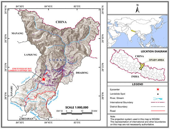
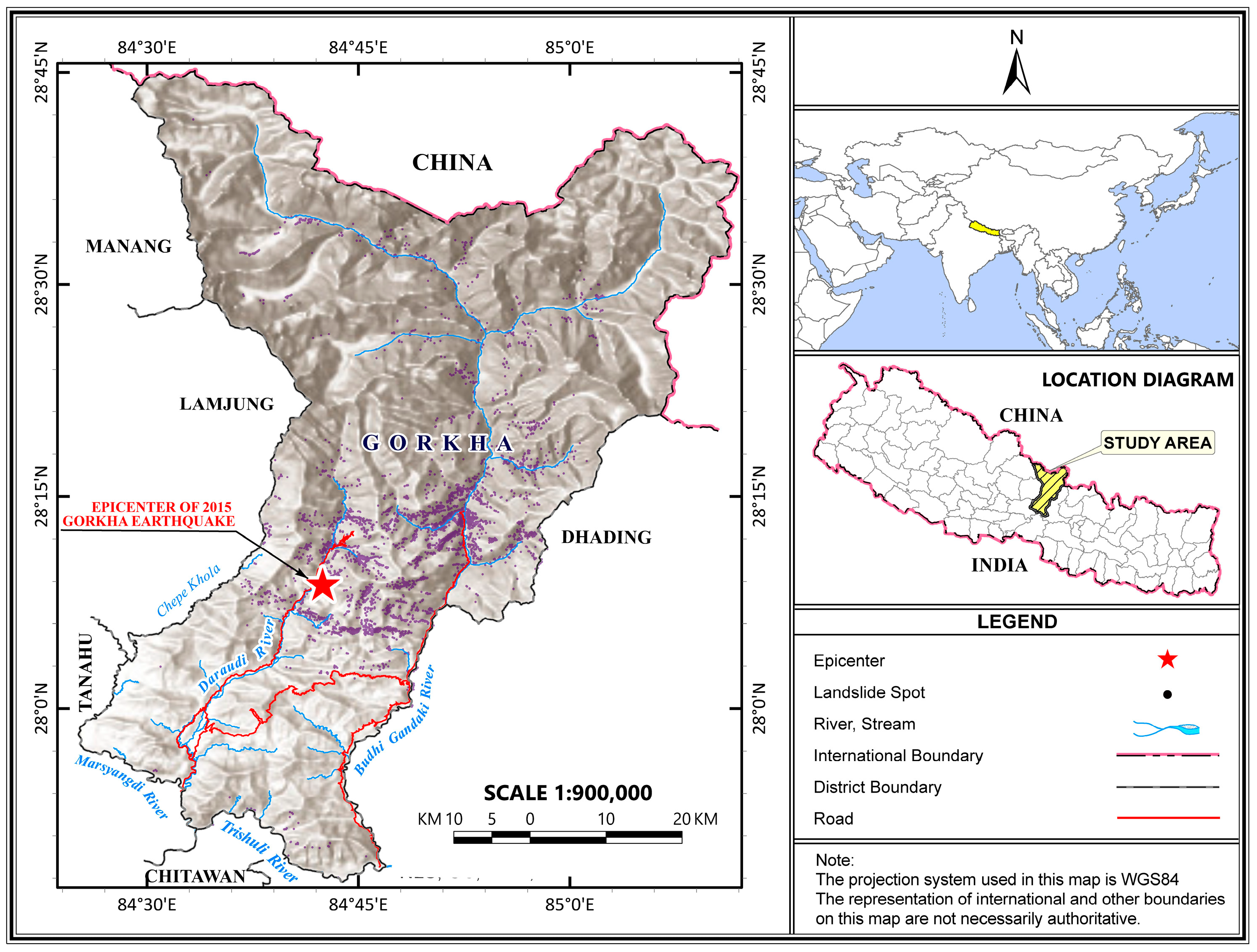
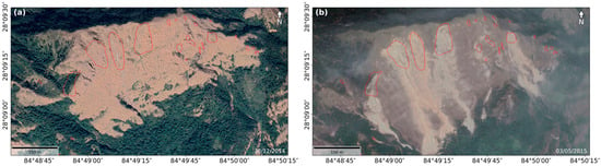
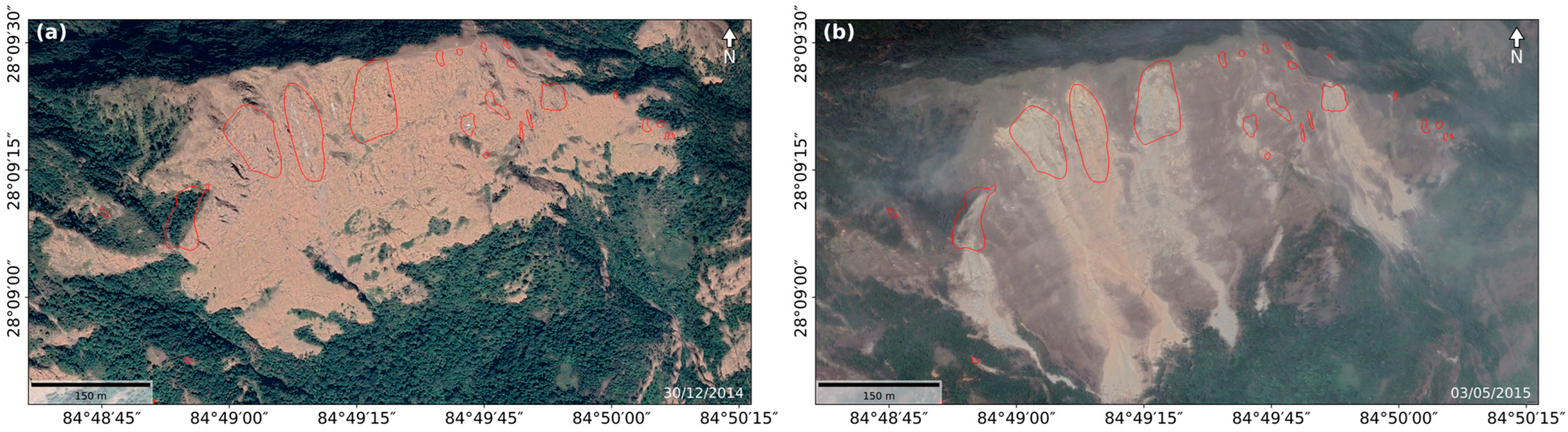
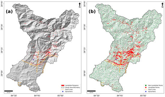
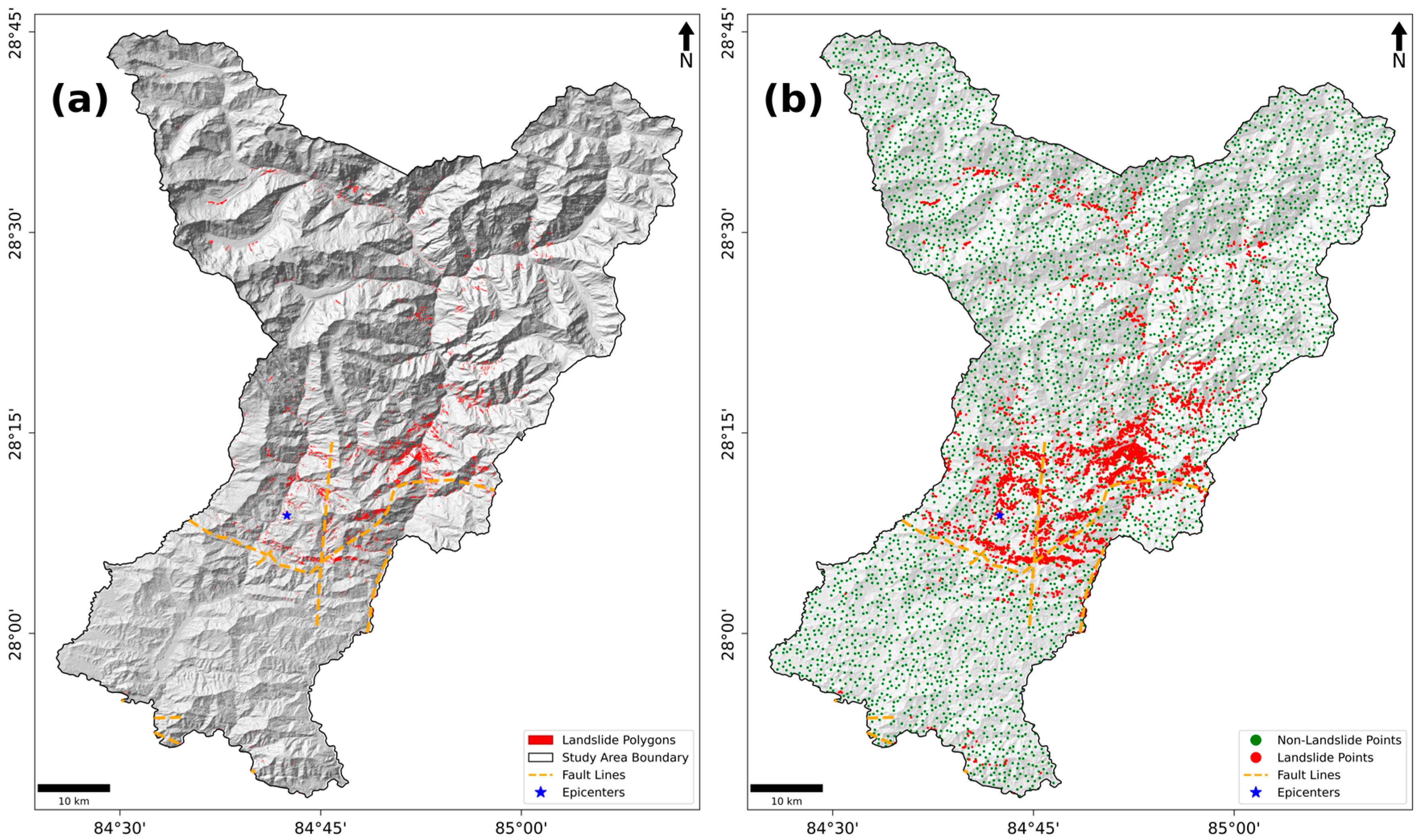
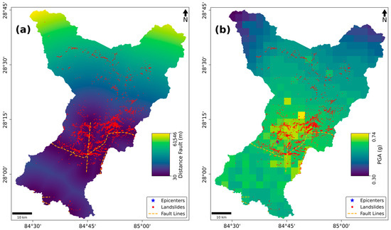
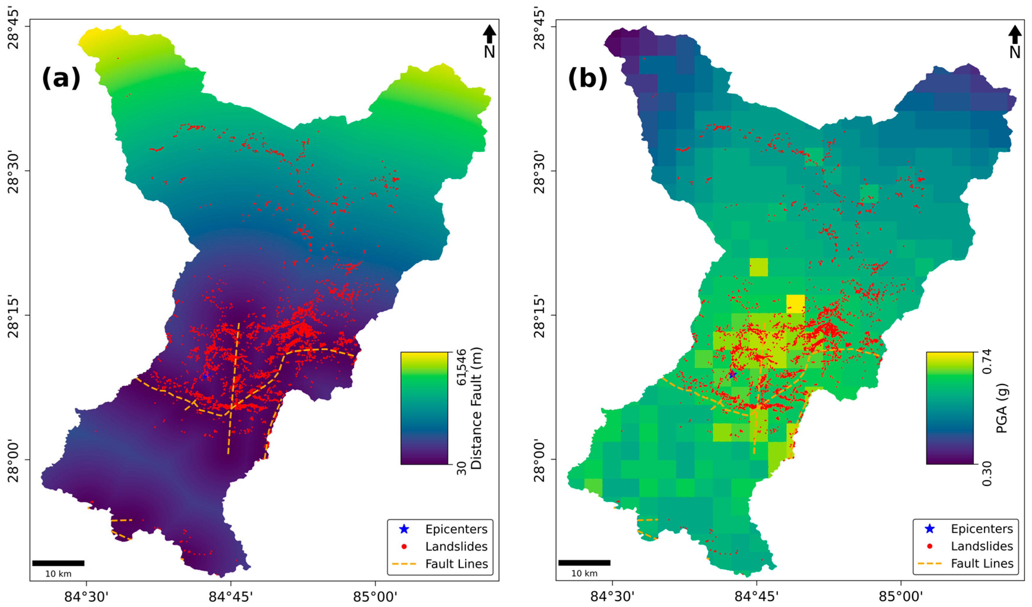
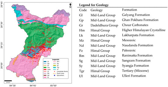
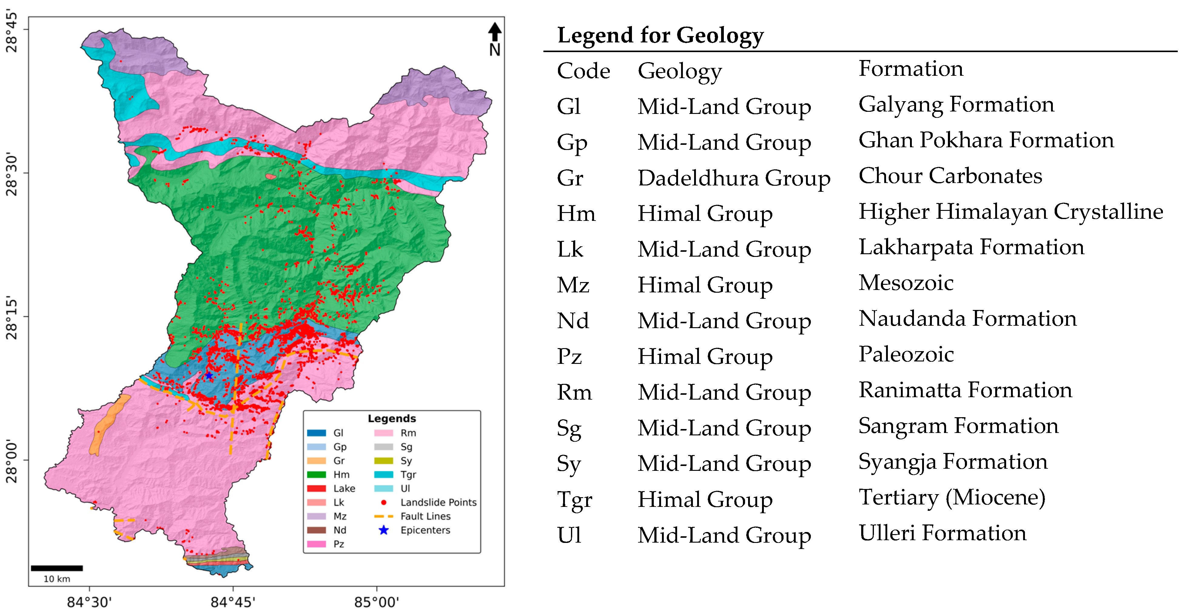
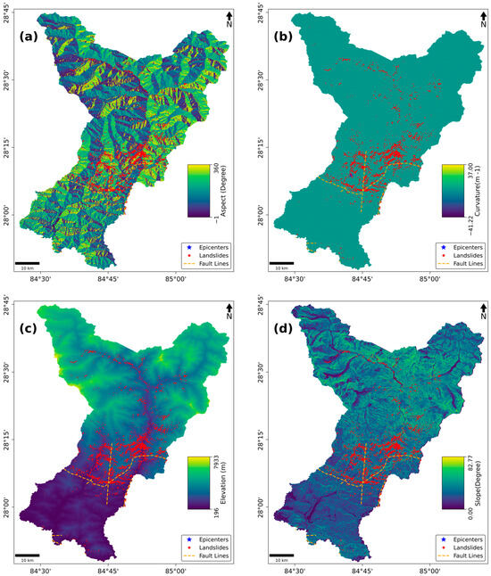
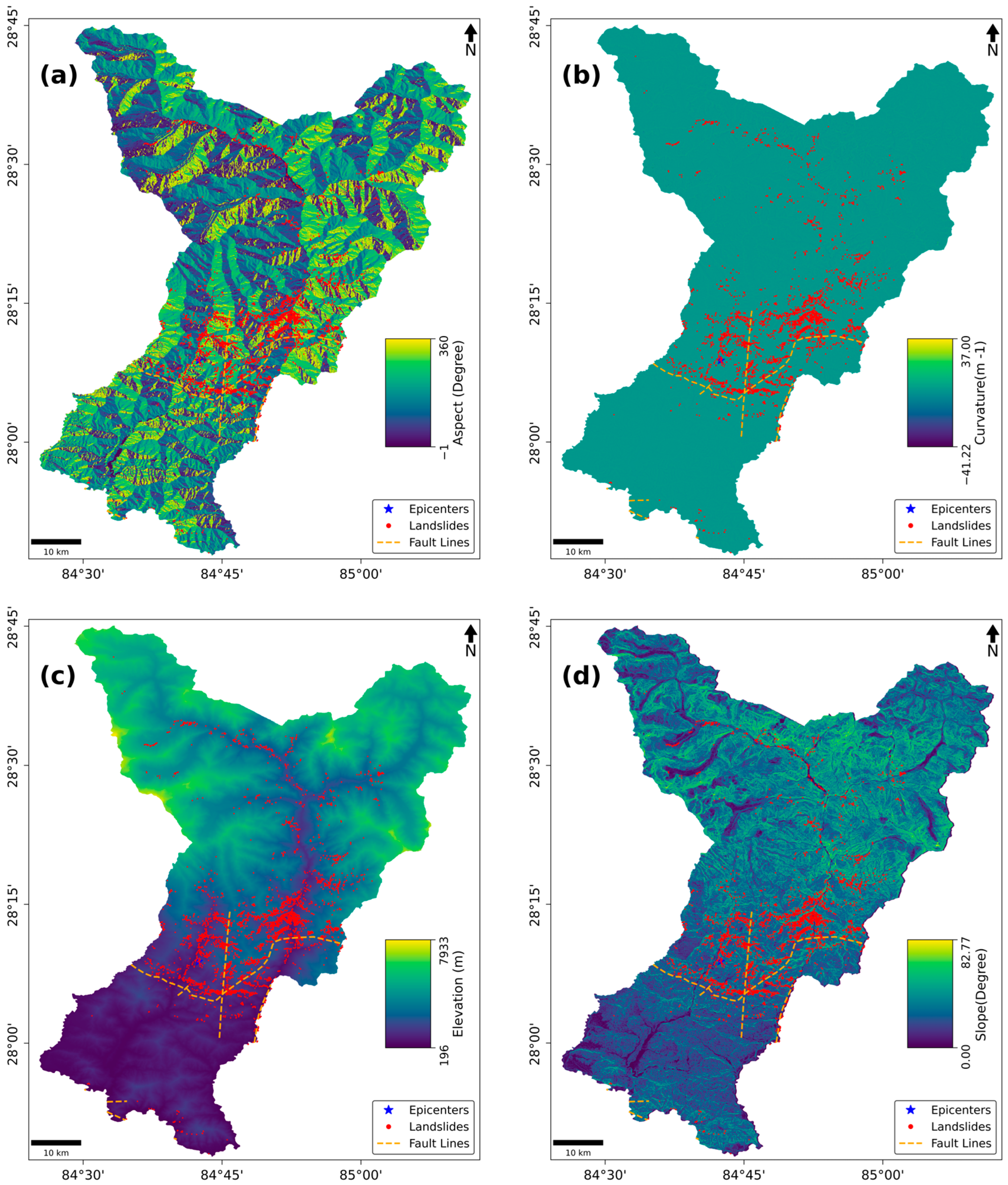
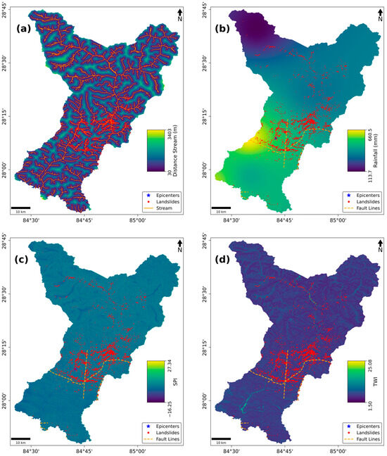
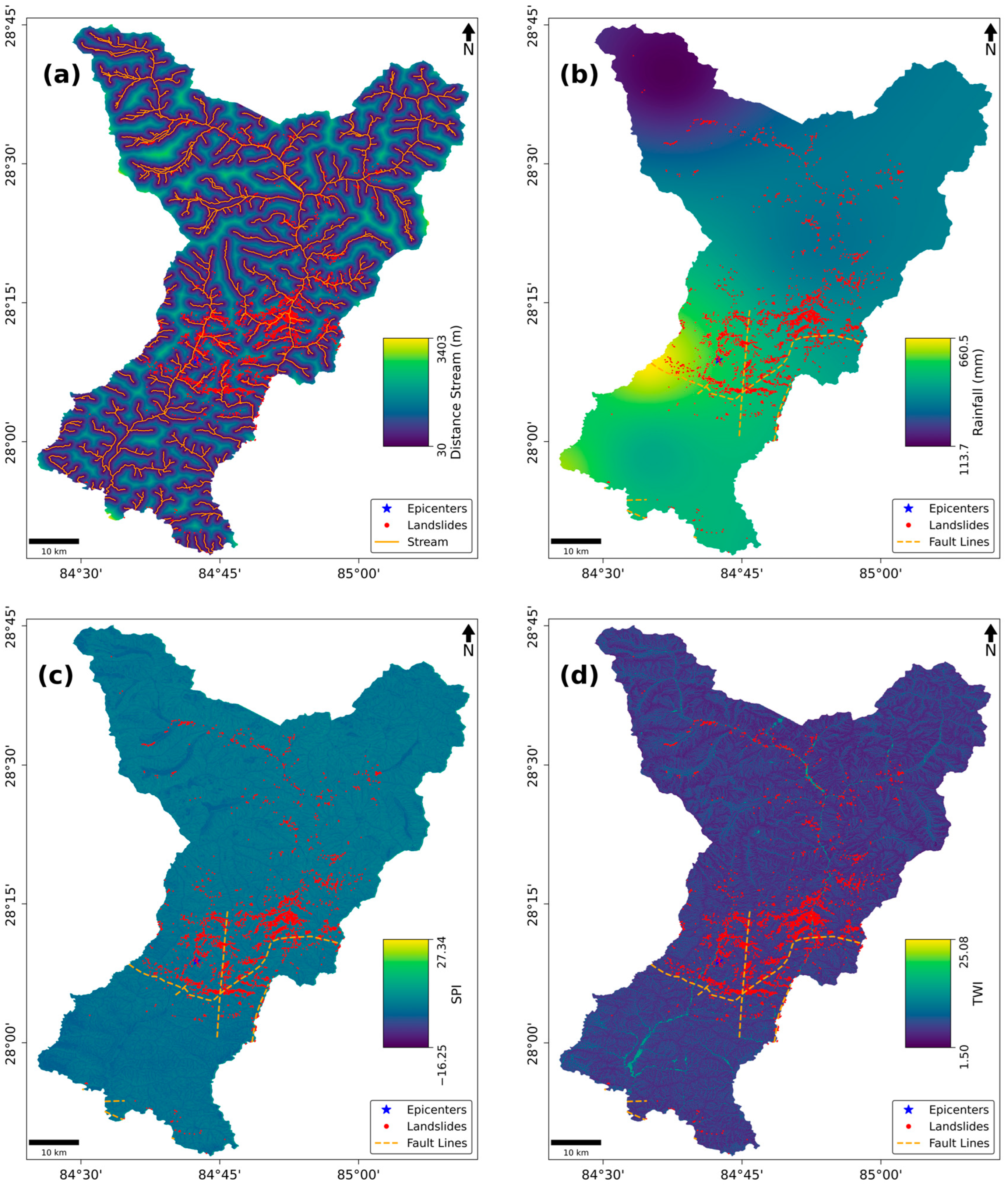
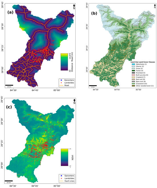
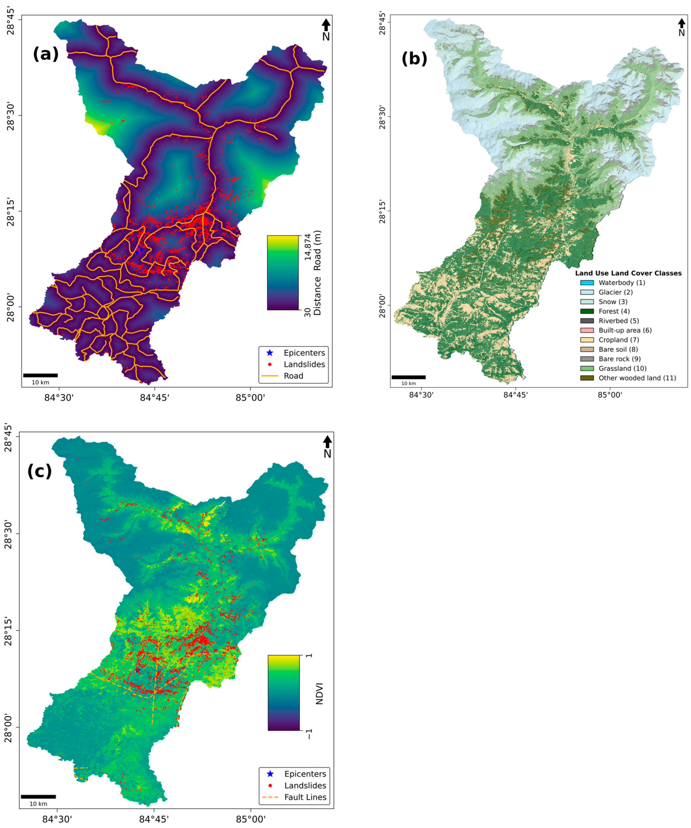
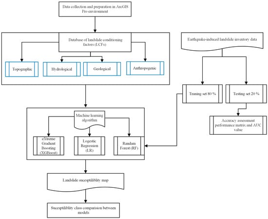
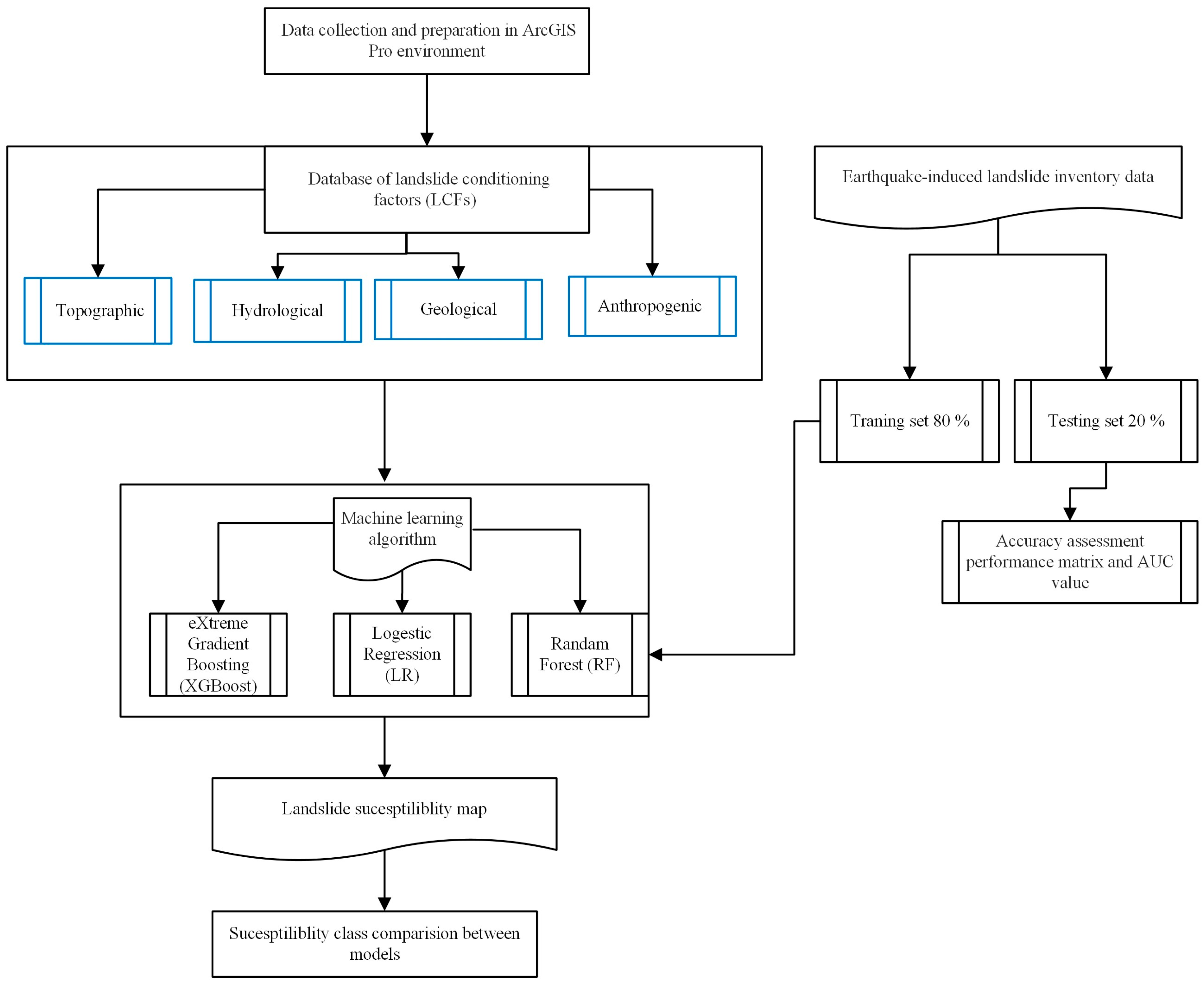
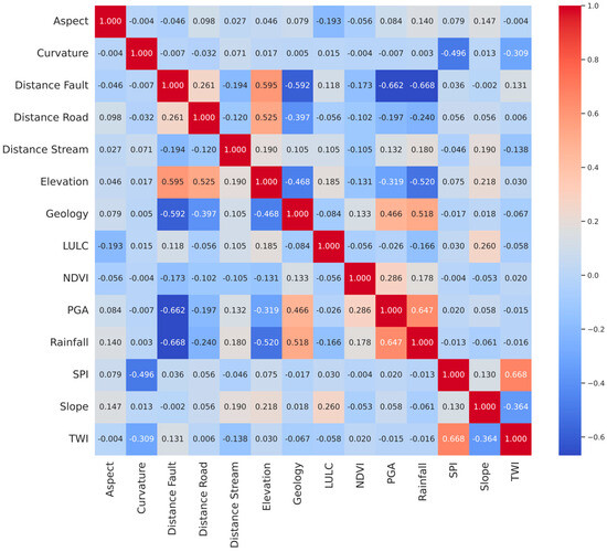
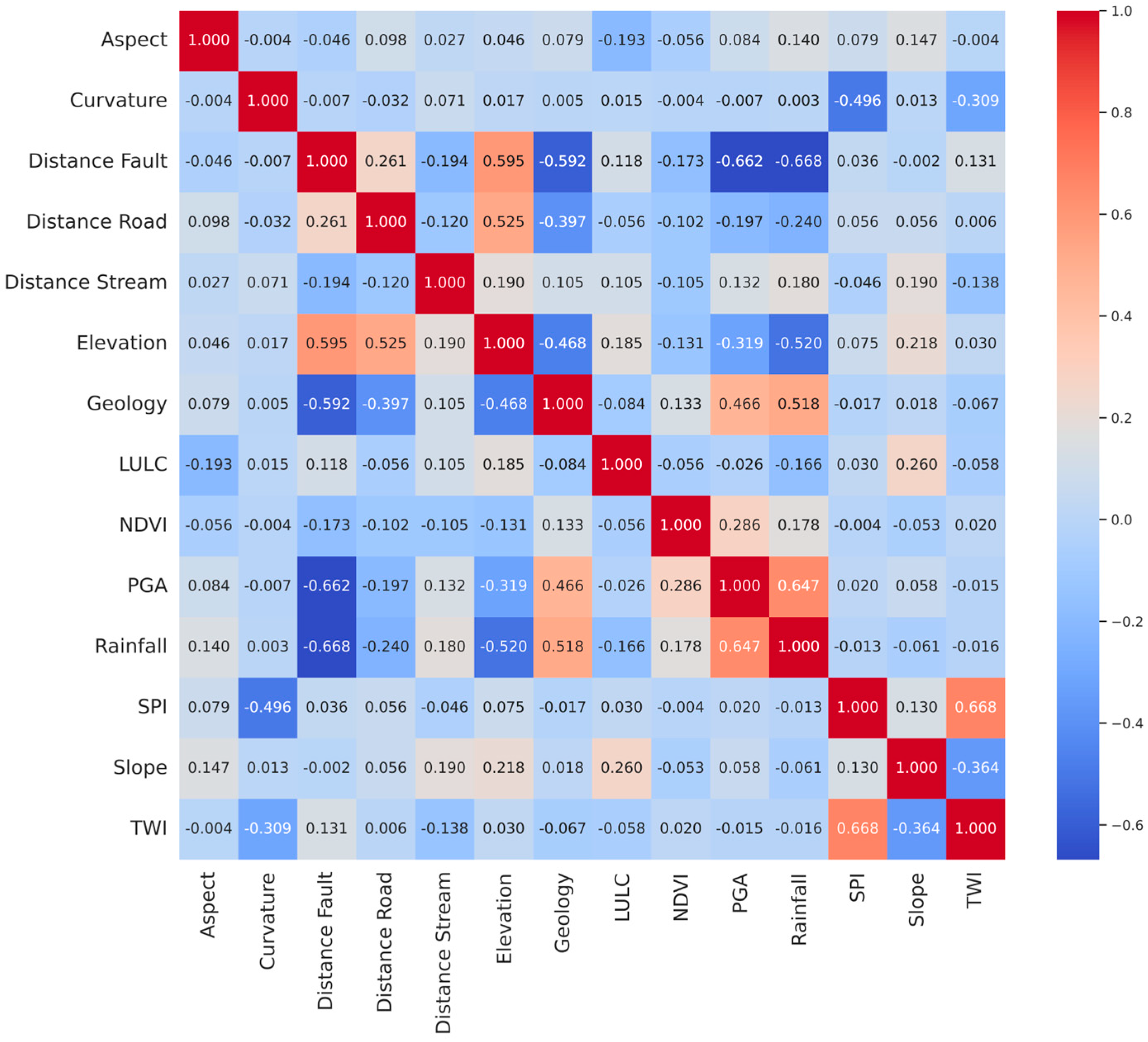
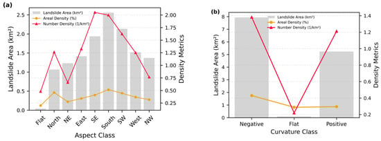
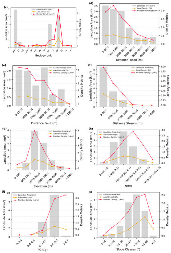
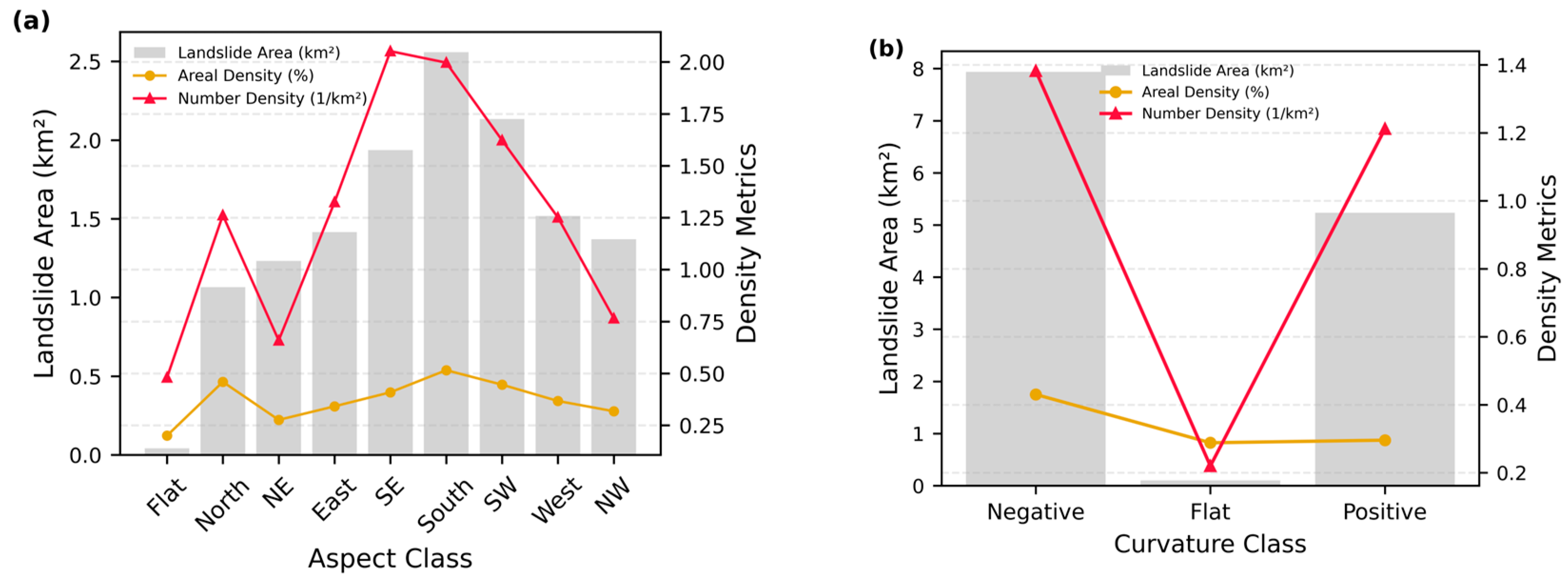
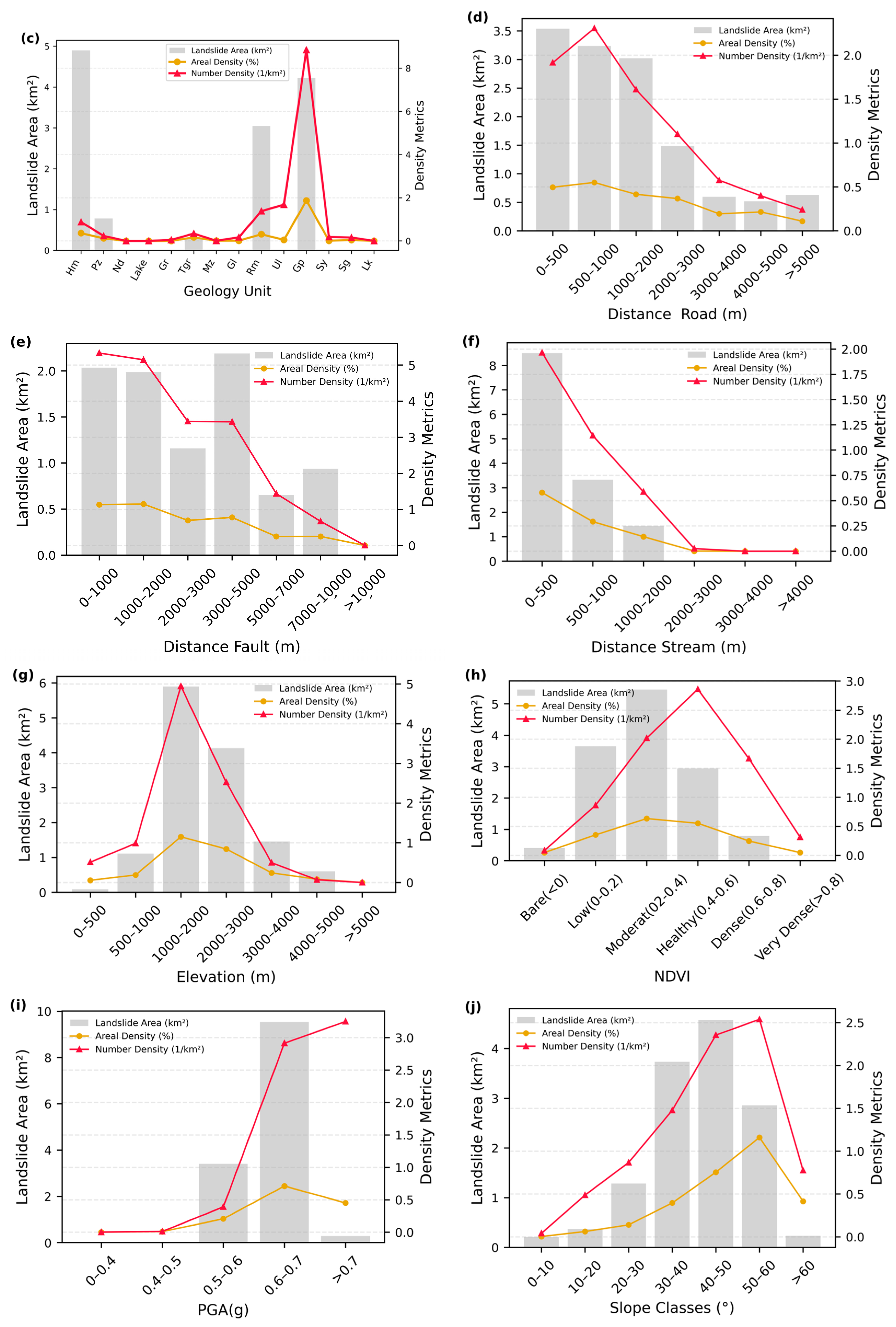
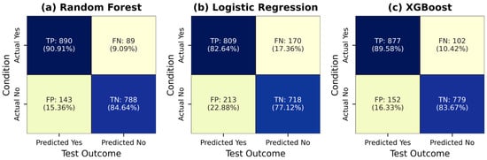
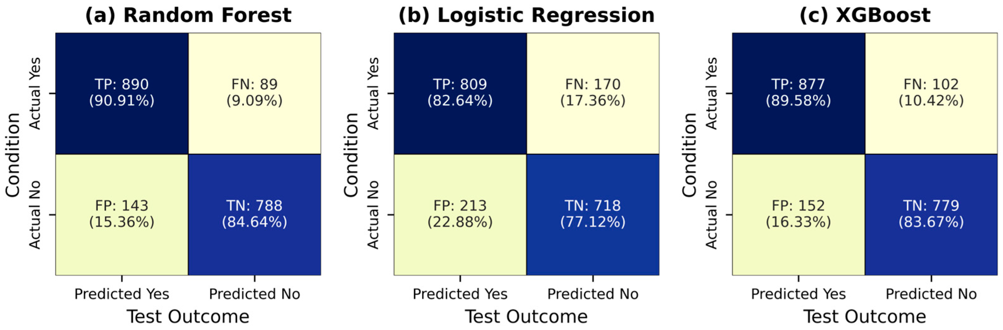
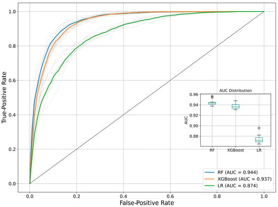
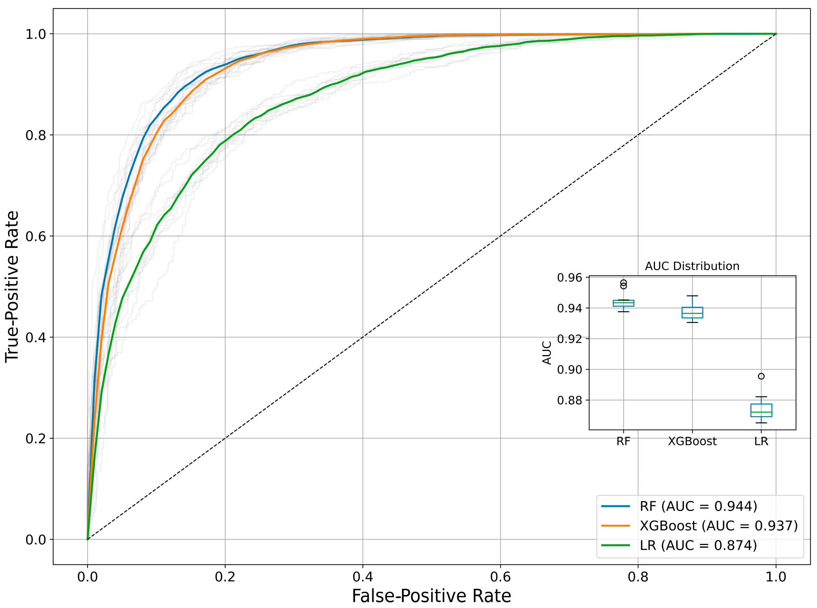
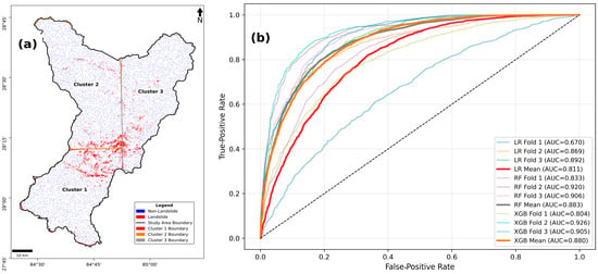
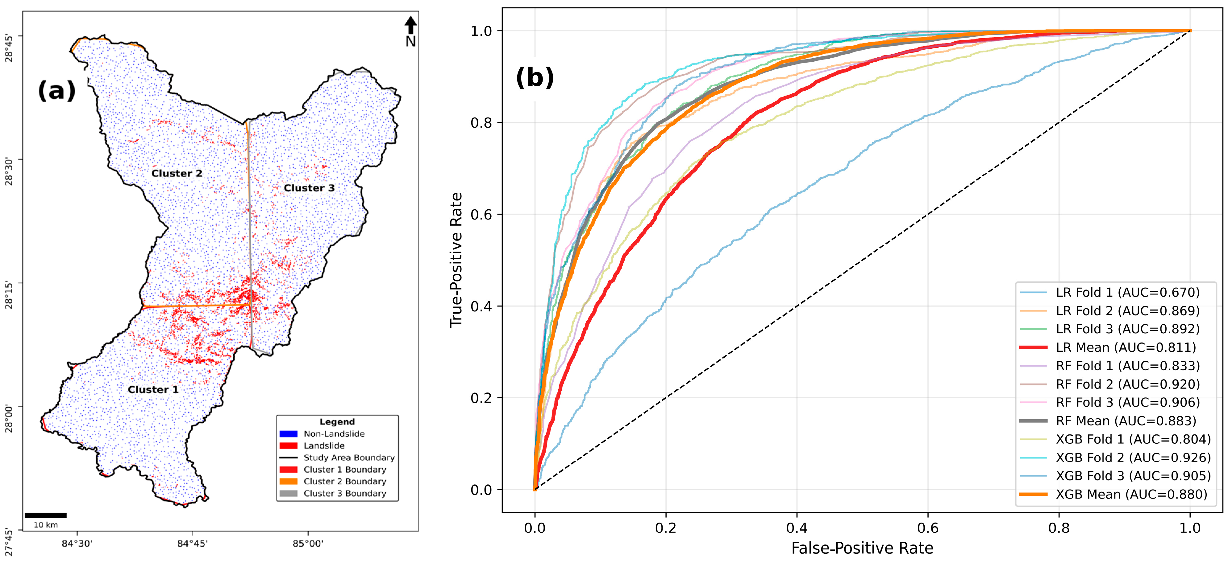
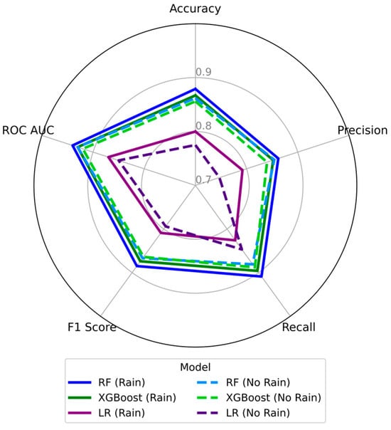
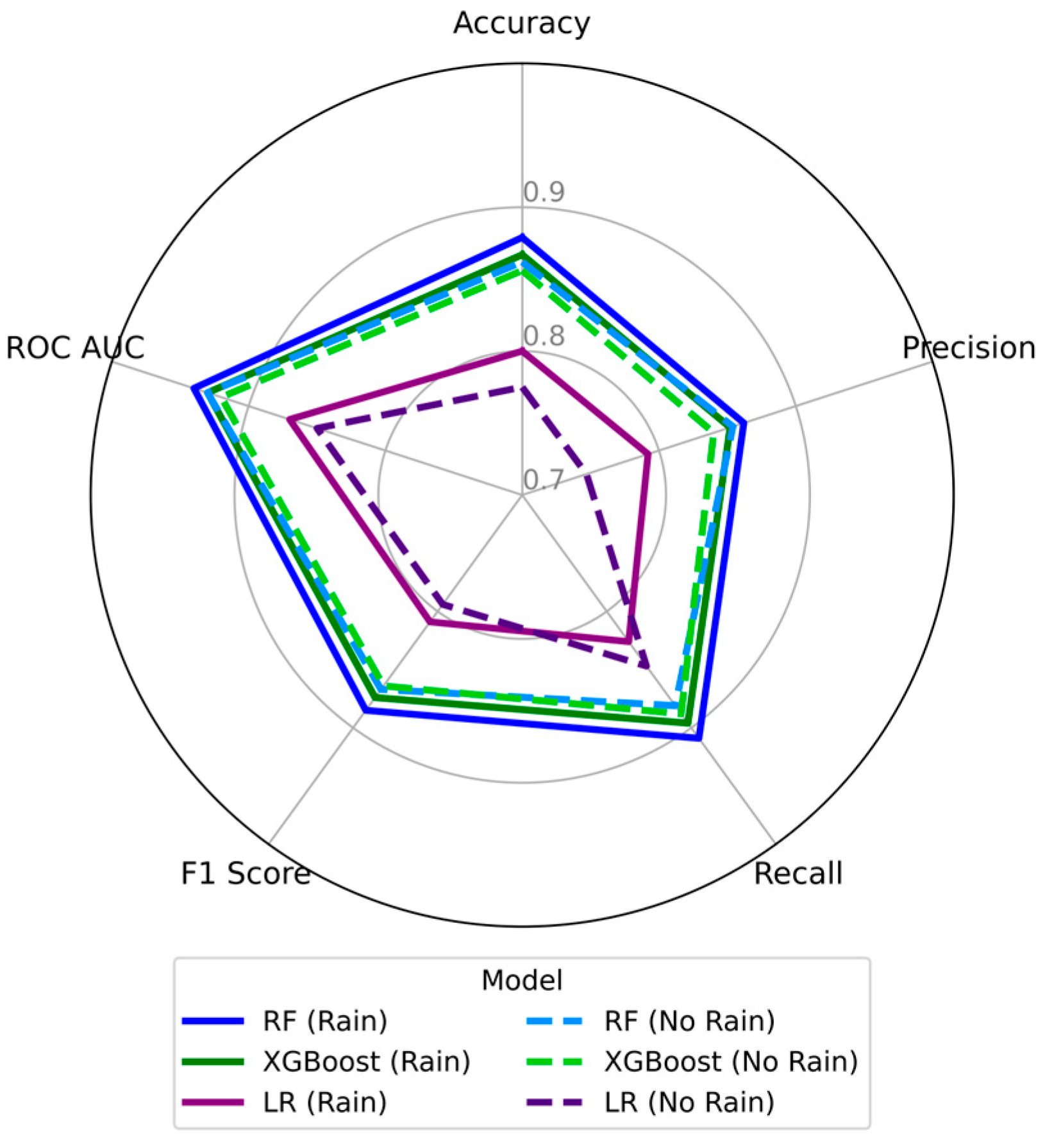
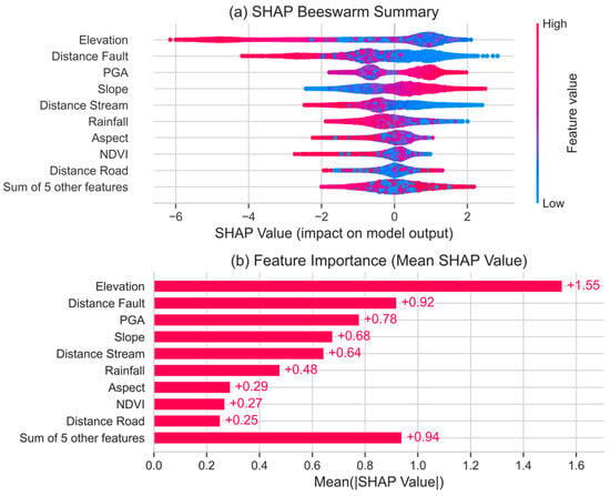
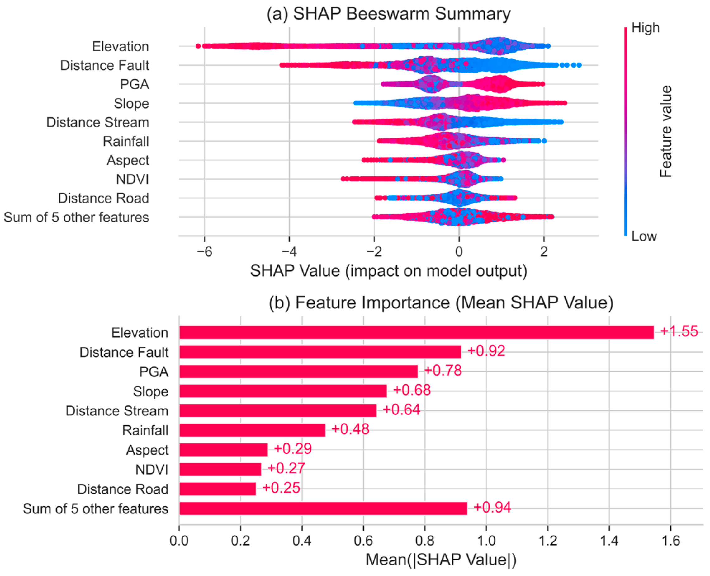
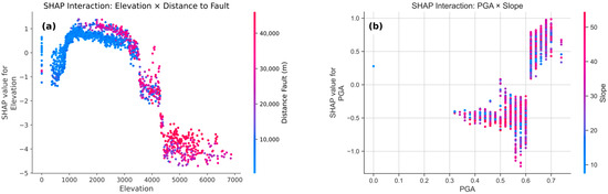
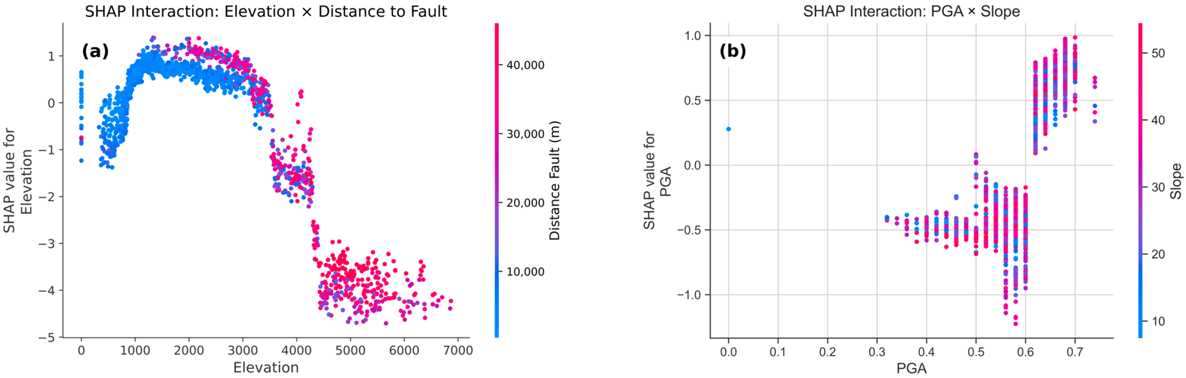
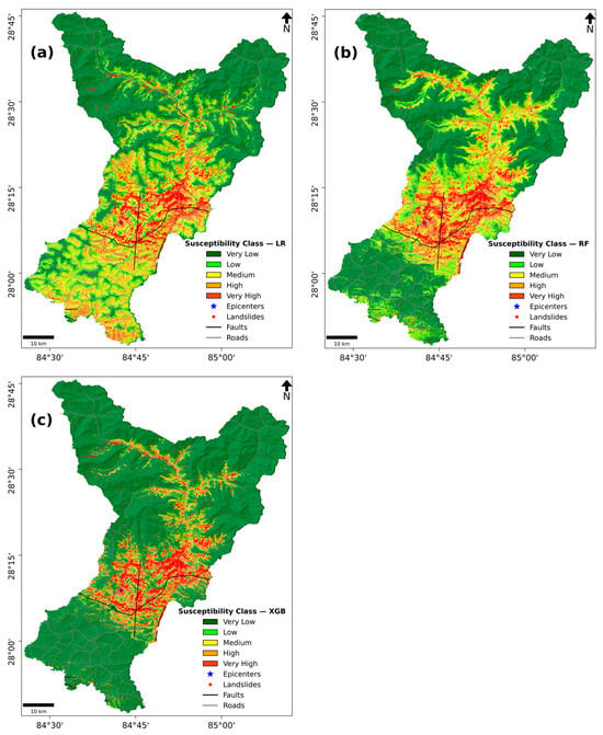
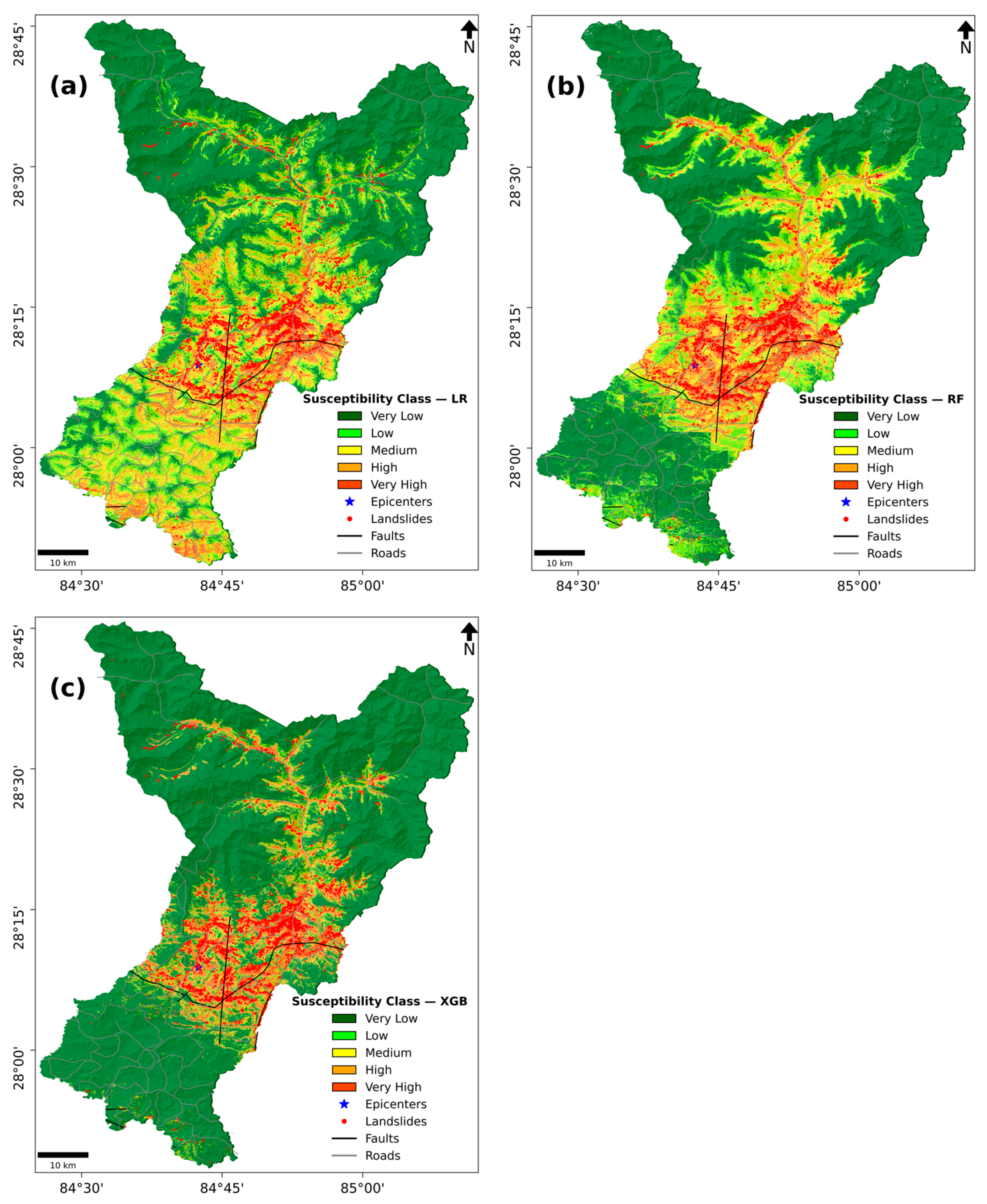
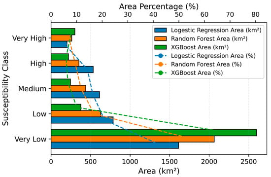
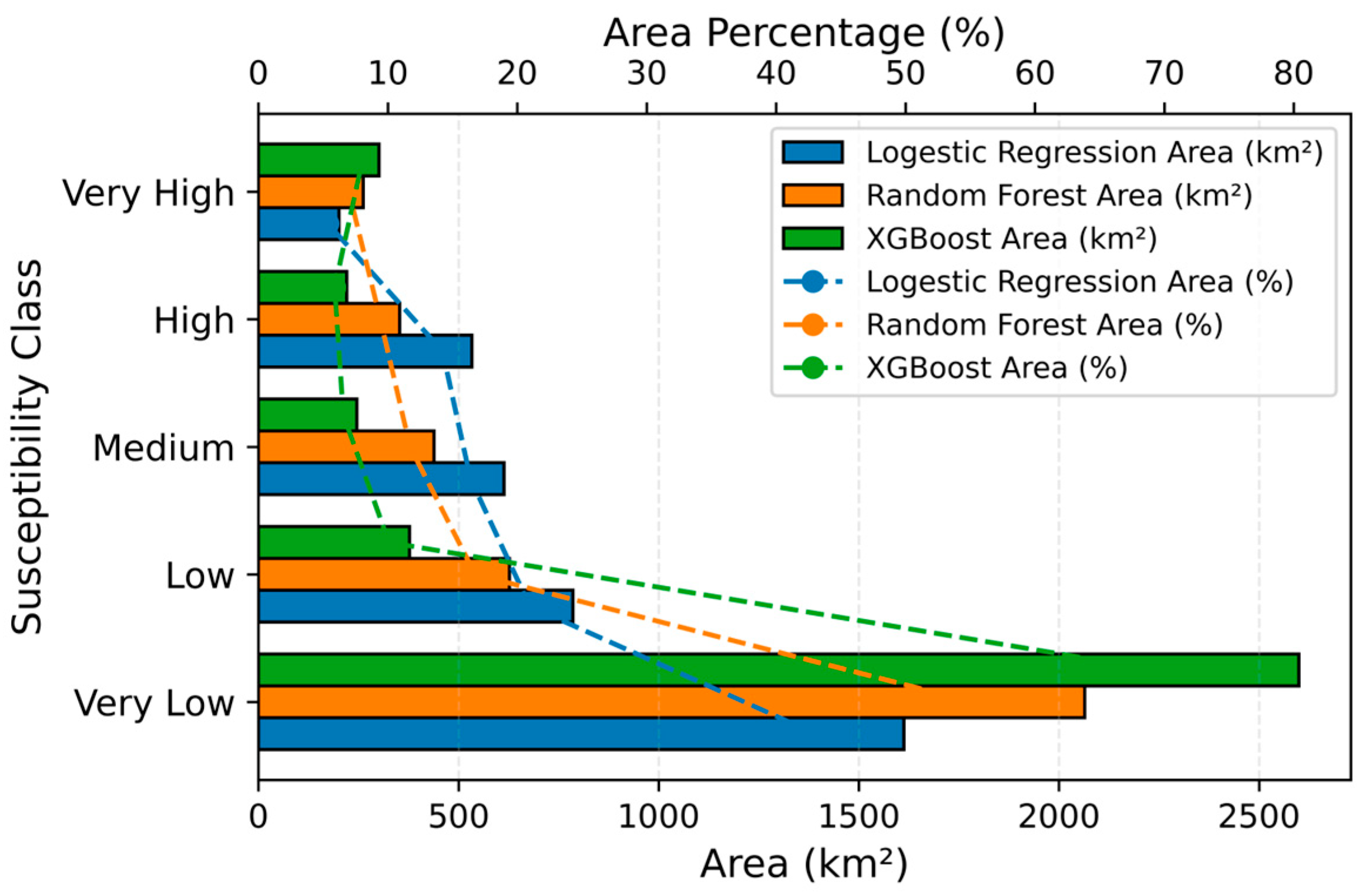
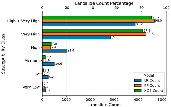
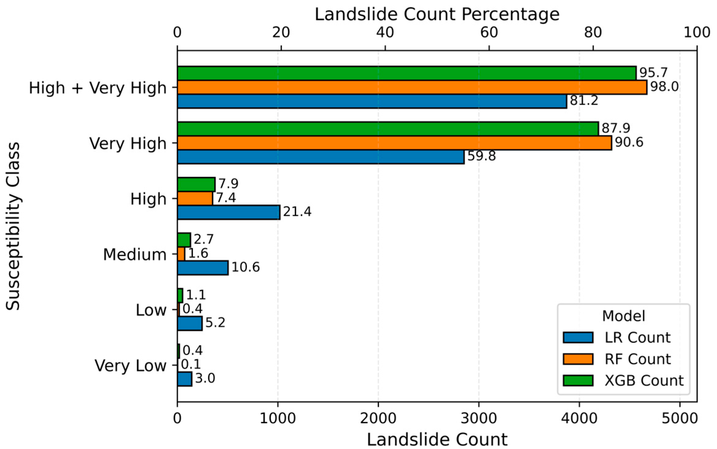
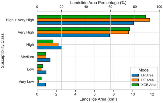
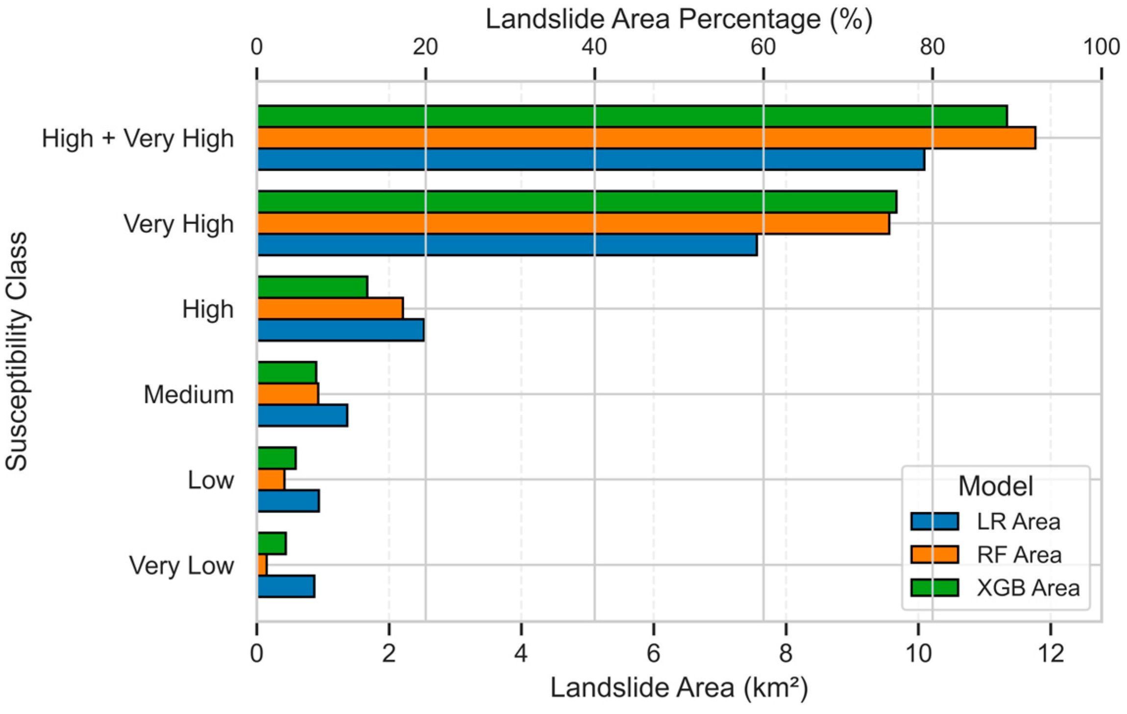
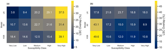
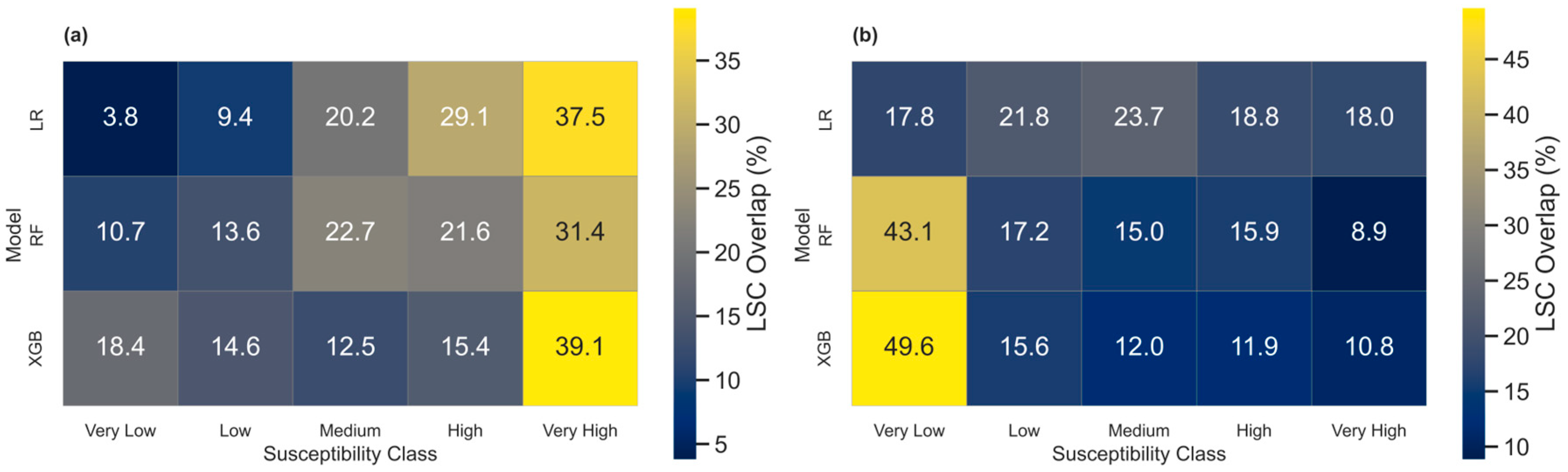

Disclaimer/Publisher’s Note: The statements, opinions and data contained in all publications are solely those of the individual author(s) and contributor(s) and not of MDPI and/or the editor(s). MDPI and/or the editor(s) disclaim responsibility for any injury to people or property resulting from any ideas, methods, instructions or products referred to in the content. |
© 2025 by the authors. Licensee MDPI, Basel, Switzerland. This article is an open access article distributed under the terms and conditions of the Creative Commons Attribution (CC BY) license (https://creativecommons.org/licenses/by/4.0/).