Unsupervised Image Classification Based on Fully Fuzzy Voronoi Tessellation

Abstract

High noise resistance and high boundary fitting accuracy have always been the goals of image classification. However, the two mutually constrain each other, making it extremely difficult to reach equilibrium. To deal with this problem, the unsupervised image classification algorithm based on fully fuzzy Voronoi tessellation is proposed. It extends Voronoi tessellation from hard to fuzzy, and proposes a hierarchical fuzzy membership model, i.e., pixels fuzzily belong to Voronoi polygons and polygons fuzzily belong to clusters. The objective function is established based on the hierarchical fuzzy membership model by fully considering the transitivity of fuzziness between different levels. Then, the optimal classification result can be obtained by the fuzzy comprehensive decision theory under the best parameter solution. The first level retains the flexibility of pixels while modeling spatial constraints. The second level determines which class the polygon belongs to under the constraint of the first level. It provides an effective way of balancing noise resistance and boundary fitting. In addition, the Voronoi tessellation is explicitly expressed in the objective function in the form of the mathematical model, which allows it to obtain the optimal value through analytical solutions instead of the previous random sampling method. It greatly increases the convergence speed of the algorithm. Experiments have been performed on simulated and several remote sensing images with seven comparing algorithms to demonstrate the effectiveness of the proposed algorithm.

1. Introduction

Image classification plays an important role in image interpretation and is widely used in many fields, such as military reconnaissance, geographic survey, and disaster assessment [1,2]. In recent years, with the rise of deep learning, a large number of image classification methods based on deep convolutional neural networks have been studied, such as FCN [3,4], U-Net [5,6], and DeepLab [7,8,9]. However, it has high requirements for the quantity and quality of samples. The generalization performance is insufficient [10]. Therefore, many researchers proposed a new idea of using unsupervised classification methods to generate pseudo-labels before deep learning [11,12]. It is beneficial for expanding the sample size and improving model performance. Thus, unsupervised image classification, as a crucial prerequisite step for the methods, is still worth challenging.

Fuzzy C-means (FCM) is of the commonly used unsupervised methods [13,14,15]. It extends hard relationships to fuzzy relationships to improve the uncertainty problem of classification. However, it has many problems when applied to image classification, such as misclassification and the salt/pepper noise phenomenon. That is because the same category in the image is not homogeneous, especially remote sensing images that have the special characteristics of the same object but different spectra [16,17]. Fortunately, images have spatial constraint characteristics, i.e., adjacent pixels in space often belong to a category. Therefore, numerous scholars focus on improving classification performance by introducing spatial constraint [18,19].

To incorporate local spatial information, Ahmed et al. proposed FCM with a spatial constraint algorithm (FCM_S) [20], which introduced a regularization term modeled by the dissimilarity of neighborhood pixels. FCM_S is more robust to noise than FCM. However, FCM_S needs to calculate neighborhood terms at each iteration, which is very time-consuming. Focusing on this problem, Chen and Zhang proposed FCM_S1 and FCM_S2 [21]. They replace the neighborhood term by introducing the mean image and median image in advance, respectively, which can reduce the computational cost. The classification performance of FCM_S1 and FCM_S2 is equivalent to that of FCM_S. Referring to the idea of mean image, Szilagyi et al. proposed the enhanced FCM (EnFCM) [22]. EnFCM constructed a linear weighted image of the original image based on the neighborhood information, and then the image classification was implemented based on the gray level of the linear weighted image. EnFCM is difficult to adaptively determine the strength of neighborhood effects. Thus, Cai et al. proposed the fast generalized FCM (FGFCM) [23]. FGFCM constructed a non-linear weighted image based on both spatial and gray-level information. However, EnFCM and FGFCM all need a parameter to balance detailed information and noise. The selection of this parameter is very important and difficult. To deal with this problem, Krinidis and Chatzis proposed the robust fuzzy local information C-means method (FLICM) [24]. The FLICM defined a novel fuzzy factor that is directly derived from the image, which can automatically determine the spatial and gray level relationship. However, FLICM ignored the situation where the central pixel is noisy. Gong et al. [25] proposed the reformulated FLICM (RFLICM). The RFLICM proposed a local coefficient of variation parameter to regulate this situation. RFLICM further improved the impact of noise, but it ignored the influence of spatial constraints on the relationship between the central pixel and adjacent pixels. Then, Gong et al. [26] further proposed the kernel-weighted FLICM (KWFLICM). The KWFLICM proposed a trade-off weighted fuzzy factor and used kernel metric to define the dissimilarity. KWFLICM achieved good results, but it limited the dimensionality of the input image to only one dimension. Thus, Memon and Lee [27] proposed the generalization of KWFLICM (GKWFICM). It extended the algorithm to multidimensional image processing. In addition, Zhang et al. also proposed a novel FLICM with non-local information and back projection (FLICMLNLI) [28]. FLICMLNLI combined local and non-local information to balance the robustness and the retention of details. To further improve the noise resistance, Tang et al. proposed a patch-based fuzzy local similarity C-means (PFLSCM) [29]. It used the structural similarity to model the neighborhood distance, and the local patches form to model the clustering distance. FLICMLNLI and PFLSCM are visually almost equivalent to KWFLICM. Wu and Qi also proposed a local feature-driven FLICM with kernel metric (LTPKW-FLICM) [30]. It embedded edge information by the local ternary model and improved the boundary classification effect. However, its visual effect is not as good as KWFLICM. In addition, the above algorithms only utilize one level of neighborhood information. To explore deeper neighborhood effects, Wu and Wu [31] proposed the master–slave hierarchy local information driven FCM (MSHLICM). MSHLICM proposed the master–slave neighborhood window to effectively describe the inherent relationship between the current pixel and its neighborhood pixels and incorporated it into FLICM. MSHLICM has stronger noise resistance and robustness.

The above spatial neighborhood effects are all modeled based on the pixel level, and their ability to overcome noise is limited. Zhao et al. [32] developed a new style and proposed the Voronoi tessellation and hidden Markov random field FCM (VT-HMRF-FCM). It constructed a hierarchical membership model based on the Voronoi tessellation technique. Pixels are first assigned to Voronoi polygons based on distance minimization from seed points. Then, all pixels within a polygon are considered as a whole. They are forced to share the same degree of membership. Taking the Voronoi polygons as the basic processing unit, the classification is executed by optimizing the Voronoi polygons and clustering centers based on the HMRF-FCM framework [33]. Compared with traditional region-based classification algorithms, VT-HMRF-FCM achieves the ability to optimize the region during the iterative process. On the one hand, it can avoid getting stuck in local optima to better adapt to complex scenes. On the other hand, its shape is relatively regular and compact. With the help of this idea, Li et al. further proposed adaptive distance-weighted Voronoi tessellation technology to enhance polygon flexibility [34]. However, it is worth noting that the Voronoi polygon is an implicit variable that cannot be solved analytically. Thus, the spatial random sampling method is used to find the optimal Voronoi tessellations. It only selects one polygon in each iteration, and randomly selects only one seed point in the polygon. The objective function is recalculated based on the new seed points set. If the value decreases, accept the new seed point, otherwise reject it. Although VT-HMRF-FCM has good noise resistance, the accuracy of the boundaries often depends on a large number of polygons and iterative optimization.

In order to perform classification faster and better, the unsupervised image classification based on fully fuzzy Voronoi tessellation algorithm (FVT-FCM) is proposed in this paper. It constructs a hierarchical fuzzy membership model, i.e., pixels fuzzily belong to Voronoi polygons and polygons fuzzily belong to clusters. In the first level, the objective function of fuzzy Voronoi tessellation is only modeled by spatial distance without spectra. It implements an explicit model representation of Voronoi tessellation, allowing it to obtain analytical solutions through the objective function. Additionally, the fuzzy Voronoi tessellation operation also greatly maintains the flexibility of pixels, making it advantageous for boundary classification. In the second level, the objective function of clustering is modeled by considering the transitivity of fuzzy based on the fuzzy Voronoi polygons. It decides the label of fuzzy polygons belonging to and guides fuzzy Voronoi polygon optimization in reverse. Finally, the optimal classification results can be obtained by fuzzy comprehensive decision theory under the optimal parameter solution. The validity of the proposed algorithm is demonstrated through experimental validation using the simulated image and remote sensing images with different resolutions from different sensors, such as a panchromatic image with 0.5 m from WorldView-1, multispectral image with 1 m from IKONOS, SAR with 30 m from RADARSAT-I, etc. The qualitative and quantitative analysis of the classification results indicates that the proposed algorithm achieves a good balance between effectively fitting boundaries and resisting noise.

The main contributions of this paper are summarized as follows,

(1)

The hierarchical fuzzy membership model is proposed. It can fully explore the uncertainty of classification to optimize boundaries.

(2)

It implements an explicit expression of Voronoi tessellation, which is beneficial for obtaining analytical solutions and achieving rapid parameter optimization.

(3)

It can maintain high noise resistance and detail preservation while quickly classifying.

This paper is organized as follows: Section 2 reviews the existing related works. Section 3 introduces the modeling and solving process of the proposed method. Section 4 shows the effectiveness of the proposed algorithm through image classification experiments using seven comparative algorithms. Section 5 thoroughly discusses the parameter impact, robustness, time complexity, and remaining challenges of the proposed algorithm. Section 6 is the conclusion.

2. Related Work

Fuzzy clustering is a process of iteratively solving parameters based on the objective function. The construction of the objective function directly affects the clustering accuracy. In this section, the objective functions of several related and classical algorithms are introduced, including the classical fuzzy C-means (FCM), the FCM with spatial constraint (FCM_S), the robust fuzzy local information C-means (FLICM) and reformulated FLICM (RFLICM), the kernel-weighted FLICM (KWFLICM) and generalization of KWFLICM (GKWFLICM), the master–slave hierarchy local information driven FCM (MSHLICM), and the Voronoi tessellation and hidden Markov random field FCM (VT-HMRF-FCM). They will provide a detailed demonstration of the evolution process of the objective function from independent pixel-based to spatially constrained pixel-based and then to hard region-based. The symbols used in this paper and their meanings are listed in Abbreviations.

2.1. Fuzzy C-Means (FCM)

FCM is the earliest fuzzy clustering algorithm. It borrowed the concept of membership degree to construct the clustering objective function for the first time, which expands the membership relationship from hard to fuzzy. The objective function of the subsequent algorithms are all evolved based on this. FCM’s objective function is as follows:

$$J_{\mathrm{FCM}}(U,V)={\displaystyle \sum _{i=1}^n{\displaystyle \sum _{l=1}^k{u}_{il}^{\lambda }{‖X_i-V_l‖}^2}}$$

(1)

where X = {X_i, i = 1, …, n} is the data set, X_i is the feature vector of data i, and n is the number of data. V = {V_l, l = 1, …, k} is the cluster center set, l is the index of clusters, k is the number of clusters (i.e., classes), and V_l is the feature vector of cluster l. U = {u_il, i = 1, …, n, l = 1, …, k} is the fuzzy membership; u_il needs to be satisfied in the condition ${\displaystyle \sum _{l=1}^k{u}_{il}=1,i=1,\dots ,n}$. λ is the fuzzy factor, which controls the fuzzy degree of the algorithm.

2.2. FCM with Spatial Constraint (FCM_S)

To introduce spatial information in image classification to overcome noise, the objective function of FCM_S is defined as follows:

$$J_{\mathrm{FCM}\text{\_}\mathrm{S}}(U,V)={\displaystyle \sum _{i=1}^n{\displaystyle \sum _{l=1}^k{u}_{il}^{\lambda }{‖X_i-V_l‖}^2}}+{\displaystyle \frac{\alpha }{N_R}}{\displaystyle \sum _{i=1}^n{\displaystyle \sum _{l=1}^k{u}_{il}^{\lambda }\left({\displaystyle \sum _{i^{\prime }\in {\delta }_i}{‖X_{i^{\prime }}-V_l‖}^2}\right)}}$$

(2)

where the second item is the regularization item modeled based on the neighborhood. X_i can represent the feature of pixel i in the image. δ_i = {i′, i′~i} is the set of neighbors around pixels i, ‘~’ represents neighborhood relationship, and N_R is the number of members of δ. When the central pixel is at the boundary, copying the features of the nearest pixel can be used to expand the image range. α stands for the effect of the neighbor’s term.

2.3. Enhanced FCM (EnFCM) and Fast Generalized FCM (FGFCM)

EnFCM and FGFCM are both based on image transformation. They have the same objective function,

$$J_{\mathrm{EnFCM}\text{\&}\mathrm{FGFCM}}(U,V)={\displaystyle \sum _{\iota =1}^{N_{\iota }}{\displaystyle \sum _{l=1}^k{\chi }_{\iota }{u}_{\iota l}^{\lambda }}}{‖X_{\iota }^{*}-V_l‖}^2$$

(3)

where X* = {X_i^*, i = 1, …, n} is the data set after image transformation. Assuming X* has N_ɩ grayscale level, X* also can be rewritten as X* = {X_ɩ^*, ɩ = 1, …, N_ɩ}. N_ɩ is the number of gray levels in the new image. U = {u_ɩl, ɩ = 1, …, N_ɩ, l = 1, …, k} is the fuzzy membership about the gray level, and u_ɩl needs to be satisfied in the condition ${\displaystyle \sum _{l=1}^k{u}_{\iota l}=1,\iota =1,\dots ,N_{\iota }}$.

In EnFCM, X* is a linear weighted image; it is modeled as,

$$X_i^{*}={\displaystyle \frac{1}{1+\alpha }}\left(X_i+{\displaystyle \frac{\alpha }{N_R}}{\displaystyle \sum _{i^{\prime }\in {\delta }_i}{X}_{i^{\prime }}}\right)$$

(4)

In FGFCM, X* is a non-linear weighted image. It is modeled as,

$$X_i^{*}={\displaystyle \frac{{\displaystyle \sum _{i^{\prime }\in {\delta }_i}{S}_{i{i}^{\prime }}{X}_{i^{\prime }}}}{{\displaystyle \sum _{i^{\prime }\in {\delta }_i}{S}_{i{i}^{\prime }}}}}$$

(5)

where S_ii′ is the relationship between central pixel and neighborhood pixels, and it is modeled as,

$$S_{i{i}^{\prime }}=\left\{\begin{array}{l}{S}_{i{i}^{\prime }}^S\times S_{i{i}^{\prime }}^{G}i\ne i^{\prime }\\ 0i=i^{\prime }\end{array}\right.$$

(6)

where $S_{i{i}^{\prime }}^S$ is the local spatial relationship, and $S_{i{i}^{\prime }}^G$ is the local spectral relationship.

$$S_{i{i}^{\prime }}^S=\exp \left({\displaystyle \frac{-\max (|x_i-x_{i^{\prime }}|,|y_i-y_{i^{\prime }}|)}{{\varphi }^S}}\right)$$

(7)

$$S_{i{i}^{\prime }}^G=\exp \left({\displaystyle \frac{-{‖X_i-X_{i^{\prime }}‖}^2}{{\varphi }^G\frac{1}{N_R}{\displaystyle \sum _{i^{\prime }\in {\delta }_i}{‖X_i-X_{i^{\prime }}‖}^2}}}\right)$$

(8)

where (x_i, y_i) is the two-dimensional coordinate of pixel i on the image. φ^S and φ^G are scale factors of $S_{i{i}^{\prime }}^S$ and $S_{i{i}^{\prime }}^G$, respectively.

2.4. Robust Fuzzy Local Information C-Means (FLICM) and Reformulated FLICM (RFLICM)

Focusing on the difficulty in parameter selection, FLICM proposed a fuzzy factor with constraints F_il to automatically determine the spatial and gray relationship. Then, the objective function is,

$$J_{\mathrm{FLICM}\text{\&}\mathrm{RFLICM}}(U,V)={\displaystyle \sum _{i=1}^n{\displaystyle \sum _{l=1}^k{u}_{il}^{\lambda }{‖X_i-V_l‖}^2+F_{il}}}$$

(9)

$$F_{i^{\prime }}={\displaystyle \sum _{i^{\prime }\in {\delta }_i}\frac{1}{d_{i{i}^{\prime }}^S+1}}{(1-u_{il})}^{\lambda }{‖X_{i^{\prime }}-V_l‖}^2$$

(10)

where $d_{i{i}^{\prime }}^S$ is the spatial distance.

RFLICM share the same objective function format with FLICM; it redefined F_il to distinguish whether the central pixel is a noise point or not. The new F_il is,

$$F_{il}^{\prime }=\left\{\begin{array}{ll}{\displaystyle \sum _{i^{\prime }\in {\delta }_i}\frac{1}{2+\min \left[{\left(\frac{M_{i^{\prime }}}{M_i}\right)}^2,{\left(\frac{M_i}{M_{i^{\prime }}}\right)}^2\right]}}\times {(1-u_{i^{\prime }l})}^{\lambda }{‖X_{i^{\prime }}-V_l‖}^2& M_{i^{\prime }}\ge {\overline{M}}_i\\ {\displaystyle \sum _{i^{\prime }\in {\delta }_i}\frac{1}{2-\min \left[{\left(\frac{M_{i^{\prime }}}{M_i}\right)}^2,{\left(\frac{M_i}{M_{i^{\prime }}}\right)}^2\right]}}\times {(1-u_{i^{\prime }l})}^{\lambda }{‖X_{i^{\prime }}-V_l‖}^2& M_{i^{\prime }}<{\overline{M}}_i\end{array}\right.$$

(11)

where M represents the local coefficient of variation, M_i and M_i′ are the local coefficient of variation of the central pixel and its neighboring pixels. M is defined as the ratio of variance to the square of mean. ${\overline{M}}_i$ is the mean of M_i.

2.5. Kernel-Weighted FLICM (KWFLICM) and Generalization of KWFLICM (GKWFLICM)

GKWFLICM is the general form of KWFLICM; their objective function is,

$$J_{\mathrm{KWFLICM}\text{\&}\mathrm{GKWFLICM}}(U,V)={\displaystyle \sum _{i=1}^n{\displaystyle \sum _{l=1}^k{u}_{il}^{\lambda }\left(1-K(X_i,V_l)\right)+G_{il}}}$$

(12)

$$G_{i^{\prime }}={\displaystyle \sum _{i=1}^n{\displaystyle \sum _{l=1}^k{u}_{il}^{\lambda }}}{\displaystyle \sum _{\begin{array}{l}i\ne i^{\prime }\\ i^{\prime }\in {\delta }_i\end{array}}{w}_{i{i}^{\prime }}{\left(1-u_{i^{\prime }l}\right)}^{\lambda }\left(1-K(X_{i^{\prime }},V_l)\right)}$$

(13)

where K is the kernel function modeled by the Gaussian Radial Basis Function (GRBF), and (1 − K(X_i, V_l)) is equivalent to the previous Euclidean distance ‖X_i− V_l‖². w_ii′ is the trade-off weighted fuzzy factor of the ith neighbor of the ith data. w_ii′ = w_sc × w_fc, where w_sc and w_fc are the constraints of local spatial and gray.

$$w_{sc}{\displaystyle \frac{1}{d_{i{i}^{\prime }}^S+1}}$$

(14)

$$w_{fc}=\left\{\begin{array}{ll}2+\exp \left[-\left(M_{i^{\prime }}-\overline{M}\right)\right]/{\displaystyle \sum _{i^{\prime }\in {\delta }_i}\exp \left[-\left(M_{i^{\prime }}-\overline{M}\right)\right]},& M_{i^{\prime }}<\overline{M}\\ 2-\exp \left[-\left(M_{i^{\prime }}-\overline{M}\right)\right]/{\displaystyle \sum _{i^{\prime }\in {\delta }_i}\exp \left[-\left(M_{i^{\prime }}-\overline{M}\right)\right]},& M_{i^{\prime }}\ge \overline{M}\end{array}\right.$$

(15)

where, $\overline{M}$ is the mean of M_i′.

2.6. Master–Slave Hierarchy Local Information Driven FCM (MSHLICM)

Referencing the objective function of FLICM, MSHLICM’s is defined as,

$$J_{\mathrm{MSHLICM}}(U,V)={\displaystyle \sum _{i=1}^n{\displaystyle \sum _{l=1}^k{u}_{il}^{\lambda }\left({‖X_i-V_l‖}^2+F_{il}+{\displaystyle \sum _{\begin{array}{l}{i}^{\prime }\ne i\\ i^{\prime }\in {\delta }_i\end{array}}\frac{{\left(1-u_{i^{\prime }l}\right)}^{\lambda }}{1+d_{i{i}^{\prime }}^S}{F}_{i^{\prime }l}}\right)}}$$

(16)

where F_i’l is the second level neighborhood term, i′′ is a member of δ_i′. δ_i′ is the neighborhood pixel set of pixels i′.

$$F_{i^{\prime }l}={\displaystyle \sum _{\begin{array}{l}{i}^{\prime }\ne i\\ i^{\prime }\in {\delta }_i\end{array}}{\displaystyle \sum _{\begin{array}{l}{i}^{″}\ne i^{\prime }\\ i^{″}\in {\delta }_{i^{\prime }}\end{array}}\frac{{\left(1-u_{i^{″}l}\right)}^{\lambda }}{1+d_{i^{\prime }{i}^{″}}^{\mathrm{S}}}{‖X_{i^{″}}-V_l‖}^2}}$$

(17)

2.7. Voronoi Tessellation and Hidden Markov Random Field FCM (VT-HMRF-FCM)

VT-HMRF-FCM introduces the implicit role of Voronoi tessellation in the objective function; it is,

$$J_{\text{VT-HMRF-FCM}}(U,\theta )={\displaystyle \sum _{j=1}^m{\displaystyle \sum _{l=1}^k{u}_{jl}{D}_{jl}+\eta }}{\displaystyle \sum _{j=1}^m{\displaystyle \sum _{l=1}^k{N}_j{u}_{jl}\log \frac{u_{jl}}{{\pi }_{jl}}}}$$

(18)

where U = {u_jl, j = 1, …, m, l = 1, …, k} is the polygon level fuzzy membership about Voronoi polygon j and cluster l, and u_jl needs to be satisfied in the condition ${\displaystyle \sum _{l=1}^k{u}_{jl}=1,j=1,\dots ,m}$. $D_{jl}={\displaystyle \sum _{i\in P_j}{d}_{il}}$ represents the polygon level distance between polygon j and cluster l. P_j represents jth Voronoi polygons. d_il is the distance between pixel i and cluster l. It is defined as the negative logarithm of the probability density function of Gaussian distribution. θ = {θ_l, l = 1, …, k} is the clustering center parameter, described in this algorithm as the mean and variance of a Gaussian distribution function. π_jl is the prior probability between polygon j and cluster l. It is defined according to Markov random field. N_j is the number of pixels in polygon j. η is the regularization coefficient.

$$d_{il}=-\log p(X_i|{\theta }_l)$$

(19)

$${\pi }_{jl}={\displaystyle \frac{\exp \left[\beta {\displaystyle \sum _{j^{\prime }\in {\delta }_j}\xi (L_j,L_{j^{\prime }})}\right]}{{\displaystyle \sum _{l^{\prime }=1}^k\exp \left[\beta {\displaystyle \sum _{j^{\prime }\in {\delta }_j}\xi (L_j=l^{\prime },L_{j^{\prime }})}\right]}}}$$

(20)

where ξ (A, B) is a binary function; if A = B, ξ (A, B) = 1, otherwise ξ (A, B) = 0. β indicates the strength of the neighborhood effect. L_j represents the cluster label of polygon j belongs to.

3. Proposed FVT-FCM Algorithm

Assume that an image is described by I = {I_i (x_i, y_i), i = 1, …, n}, where I_i = (I_is, s = 1, …, h) is the spectral feature vector of the ith pixel. s is the index of bands, h is the number of bands, (x_i, y_i) is the two-dimensional coordinate of pixel i in the image space, n is the total number of pixels.

3.1. Hierarchical Fuzzy Membership Model

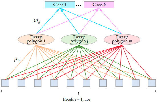
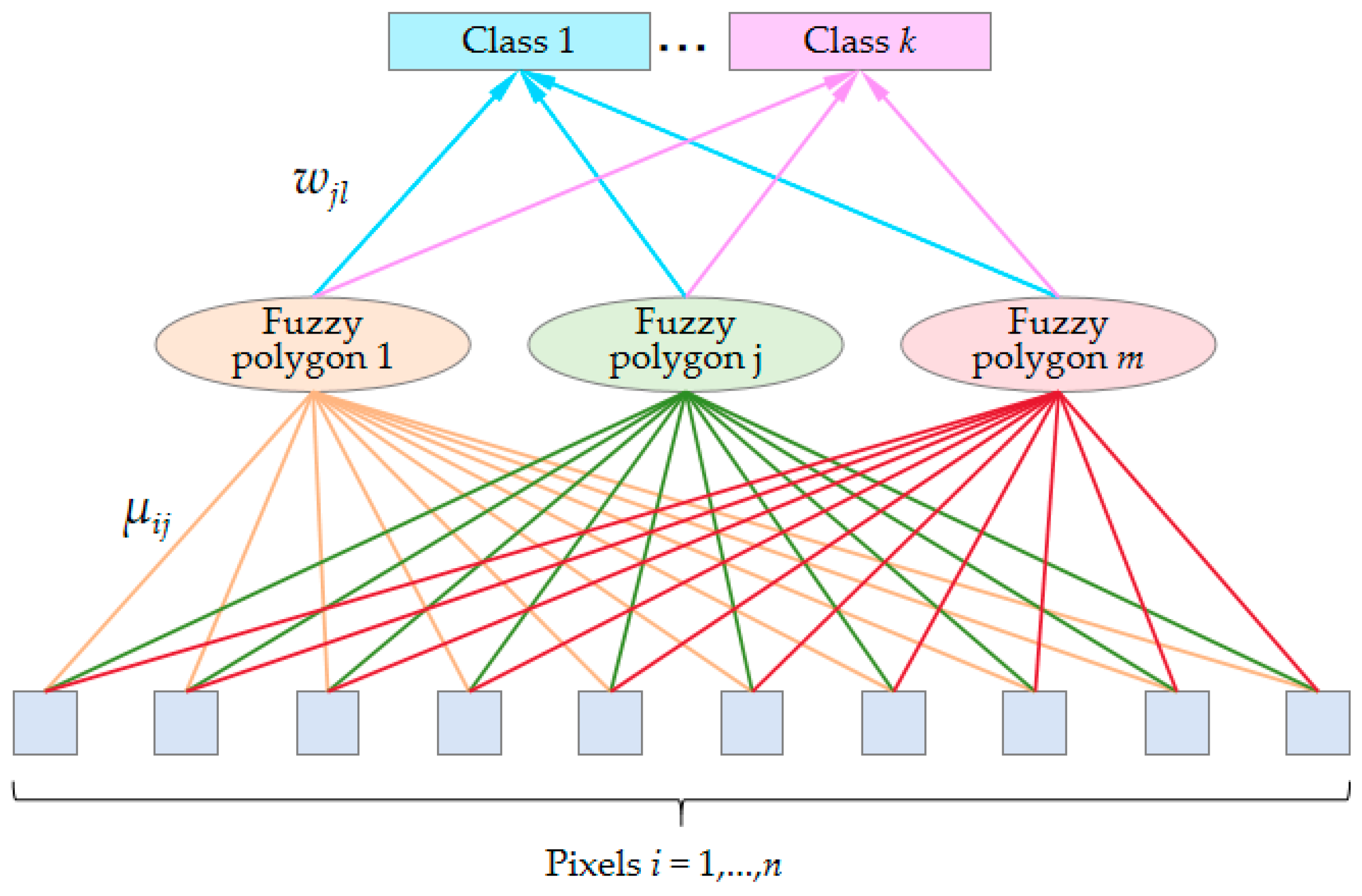
Given a seed point set C = {C_j, j = 1, …, m}, C_j = (a_j, b_j) is the two-dimensional coordinate of seed point j. The image domain is divided into m fuzzy polygons according to the fuzzy membership of pixels to polygons. The fuzzy membership is expressed as μ = {μ_ij, i = 1, …, n, j = 1, …, m}. μ_ij is also called pixel level fuzzy membership, and it needs to be satisfied in ${\displaystyle \sum _{j=1}^m{\mu }_{ij}=1,i=1,\dots ,n}$. To distinguish the label of fuzzy polygons they belong to, the polygon level fuzzy membership about fuzzy Voronoi polygon j and cluster l are also established. It is expressed as W = {w_jl, j = 1, …, m, l = 1, …, k}, ${\displaystyle \sum _{l=1}^k{w}_{jl}=1,j=1,\dots ,m}$. Then, these two fuzzy membership degrees construct a hierarchical fuzzy membership model, i.e., pixels fuzzily belong to fuzzy Voronoi polygons and fuzzy polygons fuzzily belong to clusters. The model visualization is shown in Figure 1. It shows that all pixels are related to a fuzzy polygon. Thus, this partitioning technique is also called fully fuzzy Voronoi Tessellation, where m and k are constants given empirically according to the complexity of the image.

Figure 1. Hierarchical fuzzy membership model.

3.2. Objective Function

Based on the hierarchical fuzzy membership model, there are two key points that need to be addressed. 1. How to measure the accuracy of fuzzy Voronoi tessellation. 2. How to consider fuzzy transitivity and model the relationship between fuzzy polygons and clustering. Focusing on these two difficulties, the objective function of the proposed FVT-FCM is modeled as,

$$J_{\text{FVT-FCM}}(\mu ,W,C,V)={\displaystyle \sum _{i=1}^n{\displaystyle \sum _{j=1}^m{\mu }_{ij}^{{\lambda }_1}{d}_{ij}^2+}}\eta {\displaystyle \sum _{j=1}^m{\displaystyle \sum _{l=1}^k{w}_{jl}^{{\lambda }_2}{D}_{jl}^2}}$$

(21)

where the first term is used to measure fuzzy Voronoi tessellation; it achieves the explicitly expression of tessellation. It can be regarded as a spatial clustering of two-dimensional lattice points. This term can enhance the constraint of spatially adjacent pixels. The second term is used to measure clustering based on fuzzy polygons. In this term, each pixel will participate in clustering due to the fuzzy relationship between pixels and polygons. Meanwhile, fuzzy polygons will be treated as a whole. Equation (12) greatly ensures the flexibility of pixels when establishing constraints, which provides favorable conditions for balancing noise resistance and boundary fitting. μ, W, C, V are model parameters to be solved; η is a balance coefficient. For the convenience of determining the value range, η is rewritten as q/R, q generally takes a value of 0.1, and R is a floating parameter determined by the complexity of the image. λ₁ and λ₂ are fuzzy factors for the Voronoi tessellation term and clustering term, respectively. They are usually determined empirically. If the image is fragmented, λ₁ or λ₂ are set to a smaller value. d_ij is the spatial distance between pixels and fuzzy polygons, without spectral features involved. It can be defined by the distance measure based on two-dimensional coordinates, such as the Euclidean distance.

$$d_{ij}=\sqrt{{\left(x_i-a_j\right)}^2+{\left(y_i-b_j\right)}^2}$$

(22)

D_jl is the polygon level distance between fuzzy polygons and clusters. In order to consider the transitivity of fuzzy, the pixel level fuzzy membership is introduced into the polygon level distance,

$$D_{jl}={\displaystyle \sum _{i=1}^n{\mu }_{ij}^{{\lambda }_1}{\varphi }_{il}^2}$$

(23)

where φ_il is the spectral distance between pixel i and cluster l. It can also be defined by Euclidean distance.

$${\varphi }_{i^{\prime }}={‖I_i-V_l‖}_2=\sqrt{{\displaystyle \sum _{s=1}^h{\left(I_{is}-V_{ls}\right)}^2}}$$

(24)

3.3. Parameter Estimation

According to Equation (21), there are four parameters to be solved, i.e., μ, W, C, V. Due to the constraint conditions, ${\displaystyle \sum _{j=1}^m{\mu }_{ij}=1,i=1,\dots ,n}$ and ${\displaystyle \sum _{l=1}^k{w}_{jl}=1,j=1,\dots ,m}$ need to be satisfied for parameters μ and W. Thus, Lagrange function needs to be established, and then solved using the derivative method.

$$\begin{array}{ll}L(\mu ,W,C,V)=& {\displaystyle \sum _{i=1}^n{\displaystyle \sum _{j=1}^m{\mu }_{ij}^{{\lambda }_1}{d}_{ij}^2+}}\eta {\displaystyle \sum _{j=1}^m{\displaystyle \sum _{l=1}^k{w}_{jl}^{{\lambda }_2}{\displaystyle \sum _{i=1}^n{\mu }_{ij}^{{\lambda }_1}{\varphi }_{il}^2}}}+\hfill \\ & {\displaystyle \sum _{i=1}^n{\gamma }_i\left({\displaystyle \sum _{j=1}^m{\mu }_{ij}-1}\right)}+{\displaystyle \sum _{j=1}^m{\rho }_j\left({\displaystyle \sum _{l=1}^k{w}_{jl}-1}\right)}\hfill \end{array}$$

(25)

where γ_i and ρ_j are Lagrange multipliers.

To minimize L(μ, W, C, V), it is necessary to make the partial derivatives of each parameter equal to 0,

$$\begin{gathered} {\displaystyle \frac{\partial L(\mu ,W,C,V)}{\partial {\mu }_{ij}}}=0,{\displaystyle \frac{\partial L(\mu ,W,C,V)}{\partial w_{jl}}}=0 \\ {\displaystyle \frac{\partial L(\mu ,W,C,V)}{\partial C_j}}=0,{\displaystyle \frac{\partial L(\mu ,W,C,V)}{\partial V_l}}=0 \end{gathered}$$

(26)

(1)

For parameter μ_ij,

$${\displaystyle \frac{\partial L(\mu ,W,C,V)}{\partial u_{ij}}}={\lambda }_1{\mu }_{ij}^{{\lambda }_1-1}{d}_{ij}^2+\eta {\lambda }_1{\mu }_{ij}^{{\lambda }_1-1}{\displaystyle \sum _{l=1}^k{w}_{jl}^{{\lambda }_2}{\left(I_i-V_l\right)}^2}+{\gamma }_i=0$$

(27)

Thus, we can obtain,

$${\mu }_{ij}={\displaystyle \frac{{\left(-{\gamma }_i\right)}^{\frac{1}{{\lambda }_1-1}}}{{\left[{\lambda }_1\left(d_{ij}^2+\eta {\displaystyle \sum _{l=1}^k{w}_{jl}^{{\lambda }_2}{\left(I_i-V_l\right)}^2}\right)\right]}^{\frac{1}{{\lambda }_1-1}}}}$$

(28)

According to ${\displaystyle \sum _{j=1}^m{\mu }_{ij}=1,i=1,\dots ,n}$, then,

$${\displaystyle \sum _{j^{\prime }=1}^m\frac{{\left(-{\gamma }_i\right)}^{\frac{1}{{\lambda }_1-1}}}{{\left[{\lambda }_1\left(d_{i{j}^{\prime }}^2+\xi {\displaystyle \sum _{l=1}^k{w}_{j^{\prime }l}^{{\lambda }_2}{\left(I_i-V_l\right)}^2}\right)\right]}^{\frac{1}{{\lambda }_1-1}}}=1}\text{ → }{\left(-{\gamma }_i\right)}^{{\displaystyle \frac{1}{{\lambda }_1-1}}}={\left[{\displaystyle \sum _{j^{\prime }=1}^m{\left[{\lambda }_1\left(d_{i{j}^{\prime }}^2+\eta {\displaystyle \sum _{l=1}^k{w}_{j^{\prime }l}^{{\lambda }_2}{\left(I_i-V_l\right)}^2}\right)\right]}^{-\frac{1}{{\lambda }_1-1}}}\right]}^{-1}$$

(29)

Substitute Equation (29) into Equation (28). Thus, we can obtain the solution of parameter μ_ij, that is,

$${\mu }_{ij}={\left({\displaystyle \sum _{j^{\prime }=1}^m\frac{{\left[d_{ij}^2+\eta {\displaystyle \sum _{l=1}^k{w}_{jl}^{{\lambda }_2}{\left(I_i-V_l\right)}^2}\right]}^{\frac{1}{{\lambda }_1-1}}}{{\left[d_{i{j}^{\prime }}^2+\eta {\displaystyle \sum _{l=1}^k{w}_{j^{\prime }l}^{{\lambda }_2}{\left(I_i-V_l\right)}^2}\right]}^{\frac{1}{{\lambda }_1-1}}}}\right)}^{-1}$$

(30)

(2)

For parameter w_jl,

$${\displaystyle \frac{\partial L(\mu ,W,C,V)}{\partial w_{jl}}}=\eta {\lambda }_2{w}_{jl}^{{\lambda }_2-1}{\displaystyle \sum _{i=1}^n{\mu }_{ij}^{{\lambda }_1}{\left(I_i-V_l\right)}^2+{\rho }_j}=0$$

(31)

Thus, we can obtain,

$$w_{jl}={\displaystyle \frac{{\left(-{\rho }_j\right)}^{\frac{1}{{\lambda }_2-1}}}{{\left(\eta {\lambda }_2{\displaystyle \sum _{i=1}^n{\mu }_{ij}^{{\lambda }_1}{\left(I_i-V_l\right)}^2}\right)}^{\frac{1}{{\lambda }_2-1}}}}$$

(32)

According to ${\displaystyle \sum _{l=1}^k{w}_{jl}=1,j=1,\dots ,m}$, then,

$${\displaystyle \sum _{l^{\prime }=1}^k\frac{{\left(-{\rho }_j\right)}^{\frac{1}{{\lambda }_2-1}}}{{\left(\eta {\lambda }_2{\displaystyle \sum _{i=1}^n{\mu }_{ij}^{{\lambda }_1}{\left(I_i-V_{l^{\prime }}\right)}^2}\right)}^{\frac{1}{{\lambda }_2-1}}}=1,}\text{ → }{\left(-{\rho }_j\right)}^{{\displaystyle \frac{1}{{\lambda }_2-1}}}={\left[{\displaystyle \sum _{l^{\prime }=1}^k{\left(\eta {\lambda }_2{\displaystyle \sum _{i=1}^n{\mu }_{ij}^{{\lambda }_1}{\left(I_i-V_{l^{\prime }}\right)}^2}\right)}^{-\frac{1}{{\lambda }_2-1}}}\right]}^{-1}$$

(33)

Substitute Equation (33) into Equation (32). Thus, we can obtain the solution of parameter w_jl, that is,

$$w_{jl}={\left({\displaystyle \sum _{l^{\prime }=1}^k\frac{{D_{jl}}^{\frac{1}{{\lambda }_2-1}}}{{D_{j{l}^{\prime }}}^{\frac{1}{{\lambda }_2-1}}}}\right)}^{-1}={\left({\displaystyle \sum _{l^{\prime }=1}^k\frac{{\left({\displaystyle \sum _{i=1}^n{\mu }_{ij}^{{\lambda }_1}{\left(I_i-V_l\right)}^2}\right)}^{\frac{1}{{\lambda }_2-1}}}{{\left({\displaystyle \sum _{i=1}^n{\mu }_{ij}^{{\lambda }_1}{\left(I_i-V_{l^{\prime }}\right)}^2}\right)}^{\frac{1}{{\lambda }_2-1}}}}\right)}^{-1}$$

(34)

(3)

For parameter C_j, C_j = (a_j, b_j)

$${\displaystyle \frac{\partial L(\mu ,W,C,V)}{\partial a_j}}={\displaystyle \sum _{i=1}^n{\mu }_{ij}^{{\lambda }_1}2(x_i-a_j)}=0$$

(35)

$${\displaystyle \frac{\partial L(\mu ,W,C,V)}{\partial b_j}}={\displaystyle \sum _{i=1}^n{\mu }_{ij}^{{\lambda }_1}2(y_i-b_j)}=0$$

(36)

Thus, the solution of parameter C_j is,

$$a_j={\displaystyle \frac{{\displaystyle \sum _{i=1}^n{\mu }_{ij}^{{\lambda }_1}{x}_i}}{{\displaystyle \sum _{i=1}^n{\mu }_{ij}^{{\lambda }_1}}}},b_j={\displaystyle \frac{{\displaystyle \sum _{i=1}^n{\mu }_{ij}^{{\lambda }_1}{y}_i}}{{\displaystyle \sum _{i=1}^n{\mu }_{ij}^{{\lambda }_1}}}}$$

(37)

(4)

For parameter V_l,

$${\displaystyle \frac{\partial L(\mu ,W,C,V)}{\partial V_l}}={\displaystyle \sum _{j=1}^m{w}_{jl}^{{\lambda }_2}{\displaystyle \sum _{i=1}^n{\mu }_{ij}^{{\lambda }_1}(I_i-V_l)=0}}$$

(38)

Thus, the solution of parameter V_l is,

$$V_l={\displaystyle \frac{{\displaystyle \sum _{j=1}^m{w}_{jl}^{{\lambda }_2}{\displaystyle \sum _{i=1}^n{\mu }_{ij}^{{\lambda }_1}{I}_i}}}{{\displaystyle \sum _{j=1}^m{w}_{jl}^{{\lambda }_2}{\displaystyle \sum _{i=1}^n{\mu }_{ij}^{{\lambda }_1}}}}}$$

(39)

Finally, considering the transitivity of fuzzy, the final label needs to be determined by both pixel level fuzzy membership μ_ij and polygon level fuzzy membership w_jl. According to the theory of fuzzy comprehensive decision analysis in the field of fuzzy mathematics, the matmul product is used in this paper. Then, the optimal classification label L_i can be obtained from the optimal membership μ* and W* by defuzzification operation.

$$L_i=\underset{\begin{array}{l}j=1,\dots ,m\\ l=1,\dots ,k\end{array}}{\arg \max }\left({\mu }_{ij}^{*}\times w_{jl}^{*}\right)$$

(40)

3.4. Summary of the Proposed FVT-FCM Algorithm

The proposed method is an iterative optimization algorithm for fuzzy membership. The best classification result is obtained by defuzzifying the optimal fuzzy membership. The process of the proposed FVT-FCM algorithm can be summarized as follows:

S1 Parameter initialization; include the number of polygons m, the number of classes k, the regulatory factors q and R, the fuzzy factors λ₁ and λ₂, the pixel level fuzzy membership μ⁽⁰⁾, the polygon level fuzzy membership W⁽⁰⁾, and iteration indicator t = 0;

S2 calculating the balance coefficient η;

S3 calculating C^(t) by Equation (37);

S4 calculating cluster center V_l ^(t) by Equation (39);

S5 calculating the spatial distance between pixels and fuzzy polygons d_ij ^(t) by Equation (22);

S6 calculating the polygon level distance D_jl ^(t) using Equation (23);

S7 updating W^(t) using Equation (34);

S8 updating μ^(t) using Equation (30);

S9 repeating S3–S8 until the objective function converges. When the fuzzy membership μ^(t) and W^(t) no longer change, it can be considered that the algorithm has converged.

4. Experimental Results

To verify the effectiveness of the proposed FVT-FCM algorithm, simulated and several remote sensing images are tested through qualitative and quantitative analysis based on seven comparing algorithms. These comparing algorithms are FCM, FCM_S, FGFCM, RFLICM, GKWFLICM, MSHLICM, and VT-HMRF-FCM. Here, the first four algorithms are classic fuzzy clustering algorithms, GKWFLICM and MSHLICM are the latest fuzzy clustering algorithms, VT-HMRF-FCM is the one closest to the proposed algorithm, which is also based on Voronoi tessellation.

4.1. Simulated Image

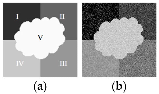
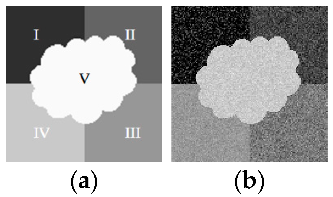
To demonstrate the effectiveness of the proposed method in noise reduction and boundary fitting more clearly, a simulated image with Gaussian distribution is generated according to the template, as shown in Figure 2. The Gaussian distribution parameters used for generating the simulated image are listed in Table 1. To simulate complexity and diversity, classes III and IV have similar means, and classes II and III, and classes IV and V have similar standard deviations.

Figure 2. (a) Template image; (b) simulated image.

Table 1. Gaussian distribution parameters used for generating the simulated image.

Parameters	Classes
	I	II	III	IV	V
Mean	20	50	100	150	200
Std.	30	20	20	10	10

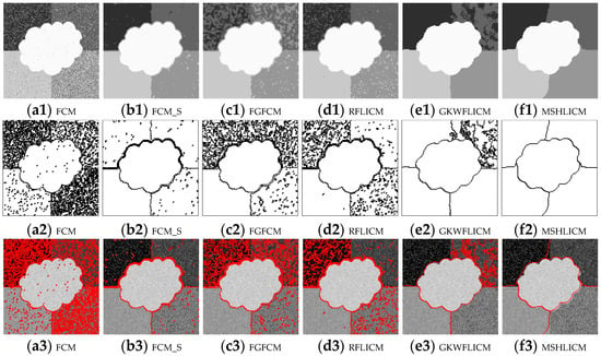
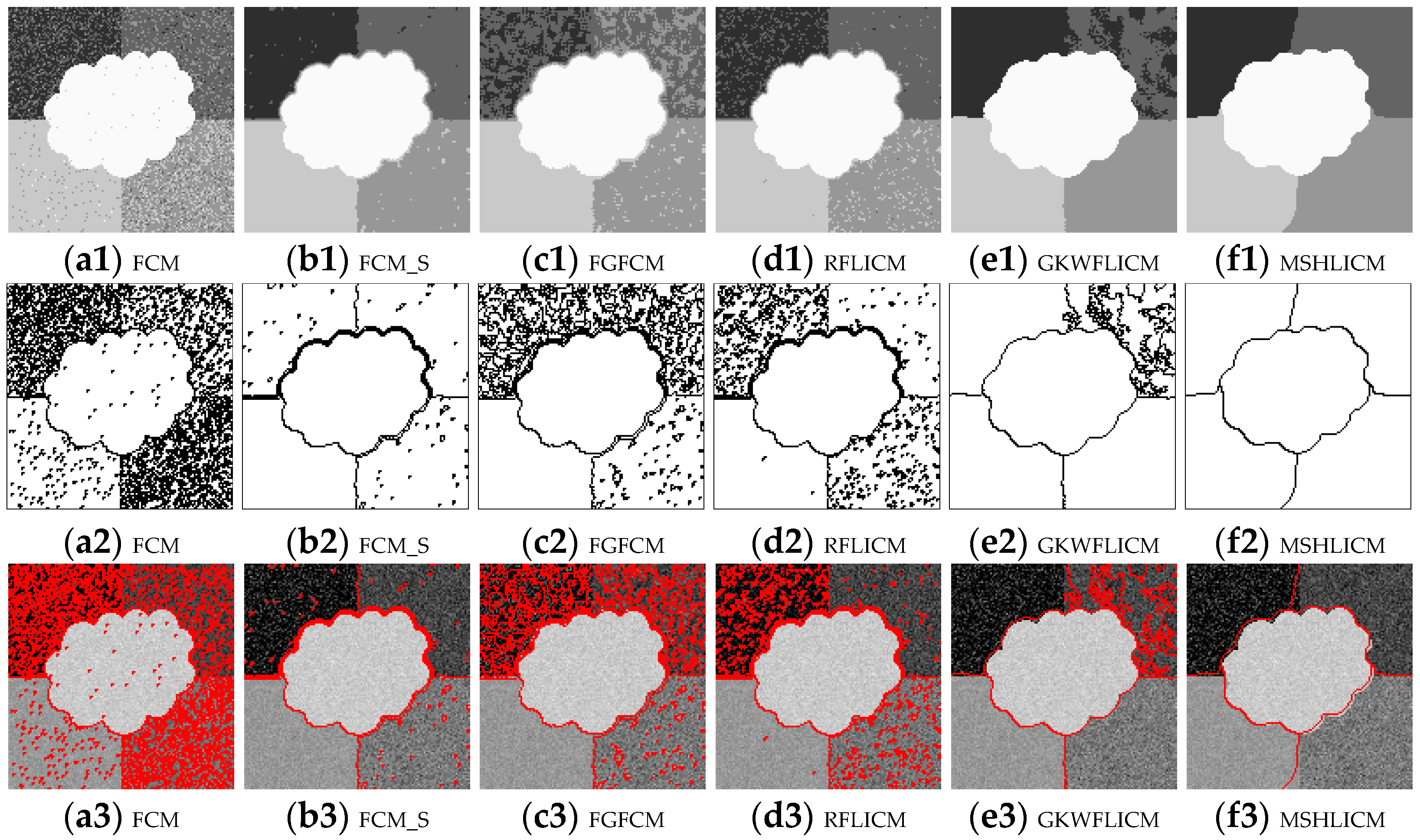
Figure 3 shows the classification results of the simulated image with pixel-based comparing algorithms, where Figure 3(a1–f1) shows FCM, FCM_S, FGFCM, RFLICM, GKWFLICM, and MSHLICM, respectively; Figure 3(a2–f2) shows the corresponding contour line images, where the content of contour lines can reflect the noise resistance level of the algorithm. Figure 3(a3–f3) shows the corresponding contour line overlay images, where the proportion of red can reflect the degree of misclassification, and the red line can also indicate the degree of fit between the classification results and the real boundaries. According to Figure 3, it can be seen that FCM is unable to classify areas with a standard deviation greater than 20, such as region I-III, as shown in Figure 3(a1–a3). FCM_S has good noise resistance, but there is still a salt and pepper phenomenon in the classification results, as shown in Figure 3(b1–b3). The classification performance of FGFCM and RFLICM are unstable. There are a large number of misclassified pixels. Additionally, due to the influence of weighted images, the classification boundaries are relatively blurry, as shown in Figure 3(c1–c3,d1–d3). GKWFLICM has overcome the salt and pepper and boundary-blurring phenomenon, but there are a large number of misclassifications in region II, as shown in Figure 3(e1–e3). MSHLICM strengthens the local constraint of neighbors through a double-layer neighborhood system, which can effectively overcome noise. However, the boundary fitting is not tight enough, as shown in Figure 3(f1–f3). To sum up, even if considering the local neighborhood constraint effect through various ways, the pixel-based clustering algorithm still yields unsatisfactory classification results.

Figure 3. Classification results of the simulated image with pixel-based comparing algorithms. (a1–f1) Classification results with FCM, FCM_S, FGFCM, RFLICM, GKWFLICM, and MSHLICM, respectively. (a2–f2) The corresponding contour line images. (a3–f3) The corresponding contour line overlay images.

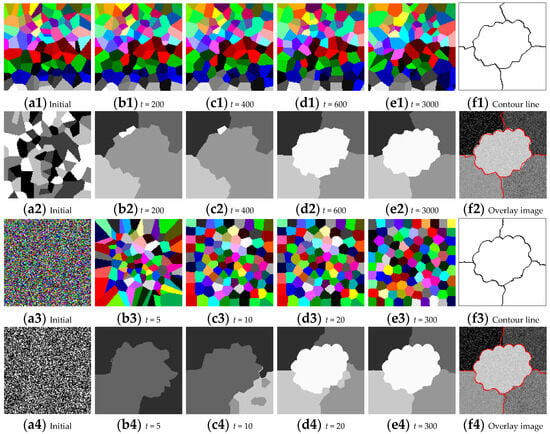
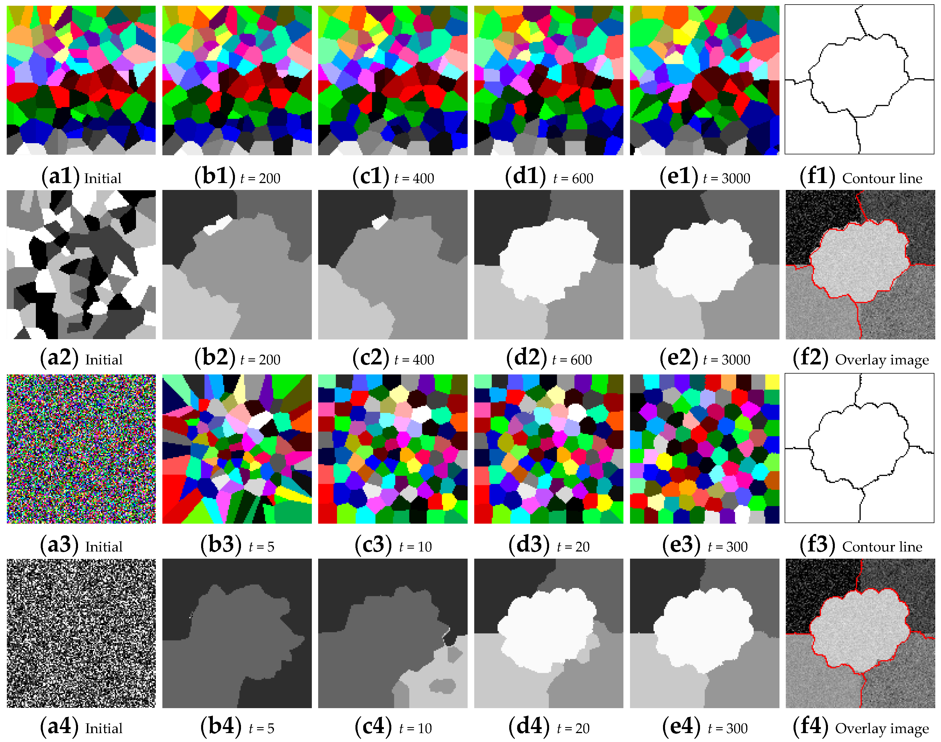
Figure 4 shows the classification result of simulated images with region-based comparing algorithm VT-HMRF-FCM and the proposed FVT-FCM, where Figure 4(a1–e1) shows the tessellation results of VT-HMRF-FCM in the initial state, 200, 400, 600, and 3000 iterations. Figure 4(a2–e2) shows the corresponding classification results. Figure 4(f1,f2) shows the contour line and overlap images of VT-HMRF-FCM, respectively. Figure 4(a3–e3) shows the tessellation results of the proposed FVT-FCM in the initial state, 5, 10, 20, and 300 iterations. Figure 4(a4–e4) shows the corresponding classification results. Figure 4(f3,f4) shows the contour line and overlap images of the proposed FVT-FCM, respectively. It can be seen that both the Voronoi tessellations and the classification results are chaotic and disorganized at the initial time. As the model iterating, the classification results gradually optimize in the correct direction. However, the optimization process of VT-HMRF-FCM is slow. The prototype appeared at 600 iterations, as shown in Figure 4(d2). This is mainly due to the lack of analytical solutions for seed points, which can only be optimized through random sampling strategies. In addition, even with sufficient iterations, VT-HMRF-FCM cannot fit the boundary well, as shown in Figure 4(f2). This is because pixels are forcibly assigned to the same polygon based on spatial distance, lacking feedback constraints from classification results, which leads to extremely inflexible polygons and makes it difficult to fit complex boundaries finely. In contrast, the prototype appears at 20 iterations in the classification result of the proposed FVT-FCM, and the best results were obtained with only 300 iterations. It benefits from the hierarchical fuzzy membership model proposed in this paper. It can effectively integrate the flexibility of pixels and the noise resistance characteristics of regions. Additionally, the Voronoi tessellation is explicitly modeled in the objective function, and it can have an analytical solution. FVT-FCM can achieve better classification with fewer iterations. To sum up, the proposed FVT-FCM can flexibly fit boundaries while having strong noise resistance.

Figure 4. Classification results of the simulated image with region-based comparing algorithm VT-HMRF-FCM and the proposed FVT-FCM algorithm. (a1–e1) Tessellation results of VT-HMRF-FCM in the initial state, 200, 400, 600, and 3000 iterations. (a2–e2) Corresponding classification results of VT-HMRF-FCM. (f1,f2) Contour line and overlap images of VT-HMRF-FCM. (a3–e3) Tessellation results of the proposed FVT-FCM in the initial state, 5, 10, 20, and 300 iterations. (a4–e4) Corresponding classification results of the proposed FVT-FCM. (f3,f4) Contour line and overlap images of the proposed FVT-FCM.

To quantitatively evaluate the effectiveness of the proposed method, the user accuracy (UA), product accuracy (PA), overall accuracy (OA), and Kappa coefficient are calculated according to the confusion matrix and listed in Table 2. It shows that the weighted image constructed by FGFCM still cannot overcome the random distribution noise, and the accuracy is the same as FCM, at only about 80%. Due to fully considering local constraints, the classification accuracy of RFLICM and GKWFLICM has been improved; OAs reach 92%. Although there is some salt and pepper noise in FCM_S, which affects the visual effect, its accuracy is 96%. MSHLICM’s accuracy remains at 96% due to boundary fitting bias issues. VT-HMRF-FCM and the proposed FVT-FCM are both region-based algorithms, they have strong noise resistance. In addition, the flexibility of fuzzy polygons demonstrates strong boundary-fitting ability, making the proposed method superior to VT-HMRF-FCM, and achieving an accuracy of up to 98.6%.

Table 2. Quantitative evaluation of simulated image classification results.

Algorithms	Accuracy	Classes
		I	II	III	IV	V
FCM	UA (%)	96.23	65.67	75.63	76.06	99.41
	PA (%)	62.38	79.98	67.03	95.98	99.34
	OA = 82.71, Kappa = 0.78
FCM_S	UA (%)	99.09	95.94	96.02	92.16	99.91
	PA (%)	95.60	96.23	96.29	99.11	96.74
	OA = 96.71, Kappa = 0.96
FGFCM	UA (%)	100	49.18	72.35	88.30	99.95
	PA (%)	39.61	60.44	93.08	99.21	95.89
	OA = 80.32, Kappa = 0.75
RFLICM	UA (%)	99.69	79.94	95.22	86.85	100
	PA (%)	77.47	95.55	89.86	99.18	97.07
	OA = 92.36, Kappa = 0.90
GKWFLICM	UA (%)	75.18	99.83	99.94	98.82	97.44
	PA (%)	95.63	65.86	99.63	99.67	99.91
	OA = 93.50, Kappa = 0.92
MSHLICM	UA (%)	100	95.66	92.83	97.59	96.03
	PA (%)	91.34	97.24	100	95.88	96.17
	OA = 96.20, Kappa = 0.95
VT-HMRF-FCM	UA (%)	96.20	97.62	96.42	99.66	99.77
	PA (%)	99.13	98.13	99.94	96.87	96.85
	OA = 98.07, Kappa = 0.97
Proposed FVT-FCM	UA (%)	99.86	96.65	99.18	98.33	98.78
	PA (%)	98.01	99.22	96.94	99.01	99.52
	OA = 98.60, Kappa = 0.98

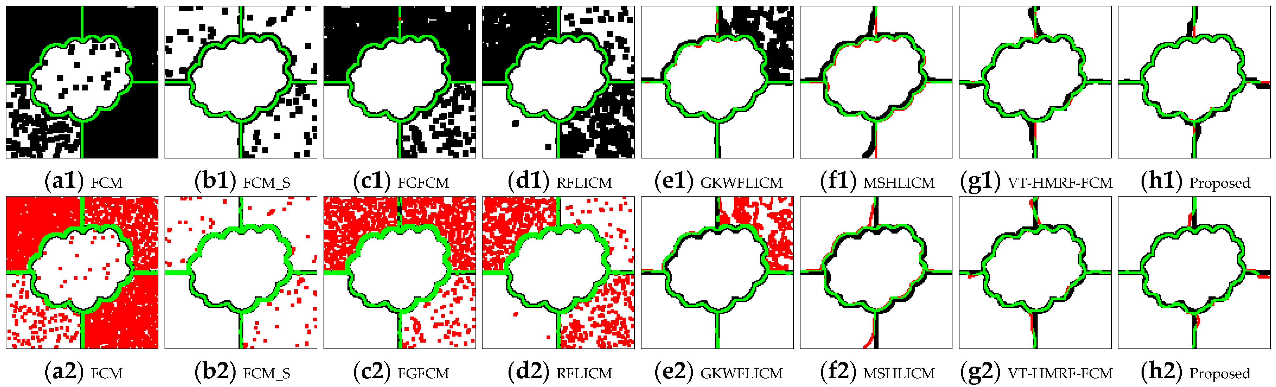
To focus on boundary effects, boundary accuracy evaluation criteria is designed based on buffer analysis in this paper. It also includes user accuracy (UA), product accuracy (PA), and overall accuracy (OA), where the UA of boundaries is the probability that the classification boundary accurately falls within the template boundary buffer area. The PA of boundaries is the probability that the template boundary accurately falls within the classification boundary buffer area. The OA is the mean of UA and PA. Figure 5 is the visualization of boundary buffer analysis, where the first row represents UA, the second row represents PA, their corresponding quantitative evaluation results are listed in Table 3. Figure 5a1,a2,b1,b2,c1,c2,d1,d2,e1,e2,f1,f2,g1,g2,h1,h2) represent FCM, FCM_S, FGFCM, RFLICM, GKWFLICM, MSHLICM, VT-HMRF-FCM, and the proposed FVT-FCM algorithm, respectively. The black represents the buffer area. The green is correct boundary pixels. The red in the first row represents the deficient boundary in classification results. The red in the second row represents the redundant boundary in classification results. It can be seen that although FCM, FCM_S, FGFCM, RFLICMA, and GKWFLICM have almost no deficient boundaries, there are a large number of redundant boundaries. It results in a larger UA and smaller PA. This extreme imbalance leads to a lower overall accuracy of the boundary, such as FCM (56.79%). On the contrary, MSHLICM sacrificed UA, resulting in a significant improvement in PA, and the OA reaches 78.15%. VT-HMRF-FCM and the proposed algorithm effectively maintained the balance between UA and PA. Both of UA and PA reach around 90%. The OA of the proposed algorithm reaches 91.74%.

Figure 5. Buffer area analysis of boundaries, where the first row represents UA, the second row represents PA.

Table 3. Boundary accuracy of simulated image classification results.

Algorithms	UA (%)	PA (%)	OA (%)
FCM	100	13.58	56.79
FCM_S	100	68.08	84.04
FGFCM	100	21.97	60.985
RFLICM	100	26.03	63.015
GKWFLICM	95.10	40.05	67.575
MSHLICM	77.95	78.35	78.15
VT-HMRF-FCM	93.43	89.21	91.32
Proposed FVT-FCM	93.88	89.60	91.74

4.2. Remote Sensing Image

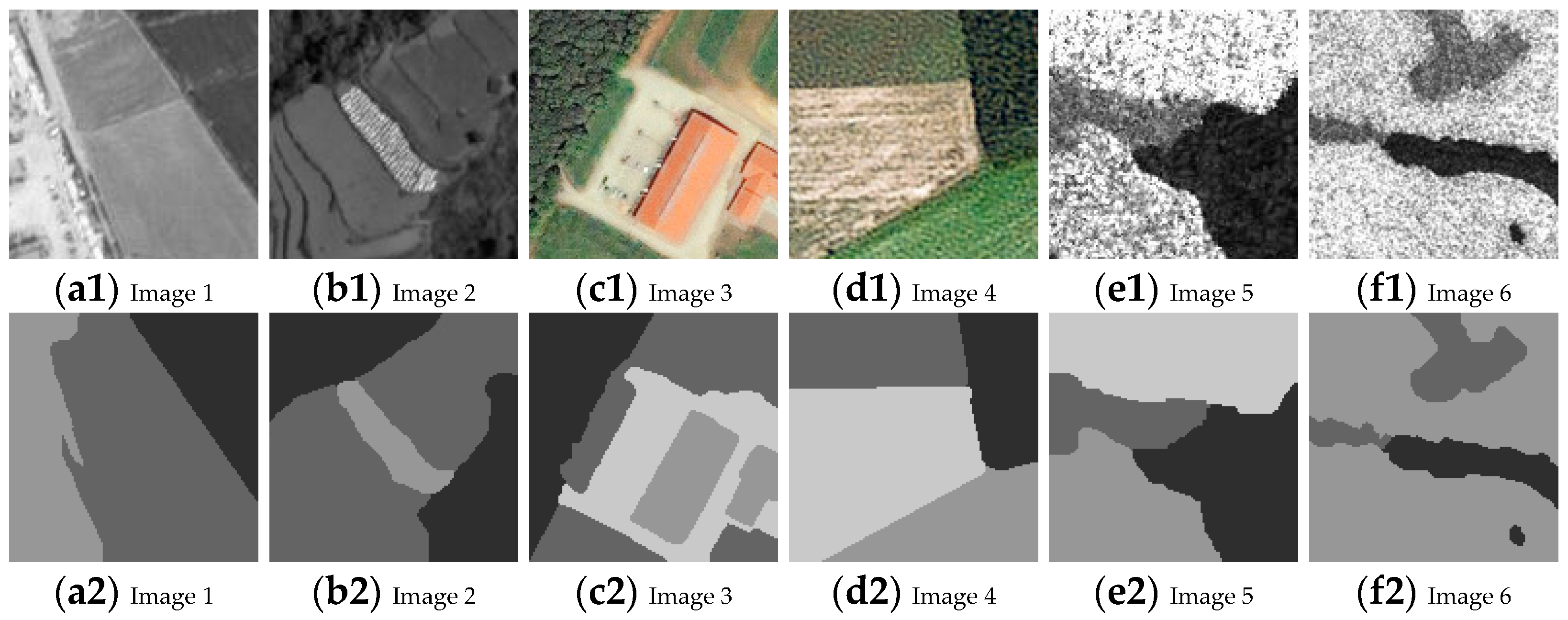
Remote sensing images are more complex than natural images, so some remote sensing images are also selected from different sensors to verify the effectiveness of the proposed algorithm, as shown in Figure 6. Figure 6(a1,b1) shows panchromatic images, Figure 6(c1,d1) shows multispectral images, and Figure 6(e1,f1) shows synthetic aperture radar (SAR) images, and their sensor parameters are listed in Table 4. Figure 6(a2–f2) shows the corresponding ground truth images.

Figure 6. Remote sensing images. (a1,b1) Panchromatic images. (c1,d1) Multispectral images. (e1,f1) SAR images. (a2–f2) Corresponding ground truth images.

Table 4. Sensor parameters of remote sensing images.

Images	Sensors	Spatial Resolution	Number of Bands
Image 1	Cartosat-1	2.5 m	1
Image 2	WordView-1	0.5	1
Image 3	IKONOS	1 m	3
Image 4	Spot-5	2.5 m	3
Image 5	RADARSAT-I	30 m	1
Image 6	RADARSAT-I	30 m	1

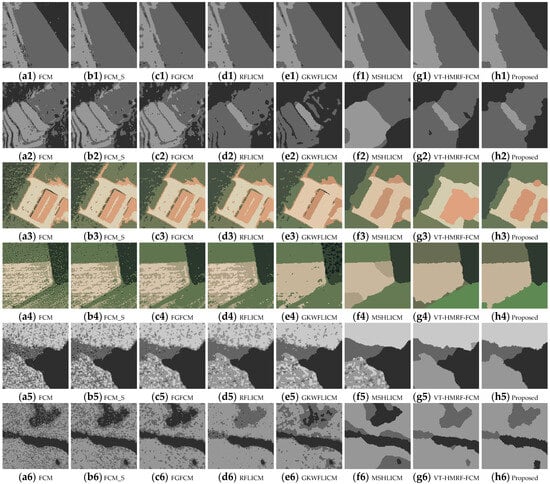
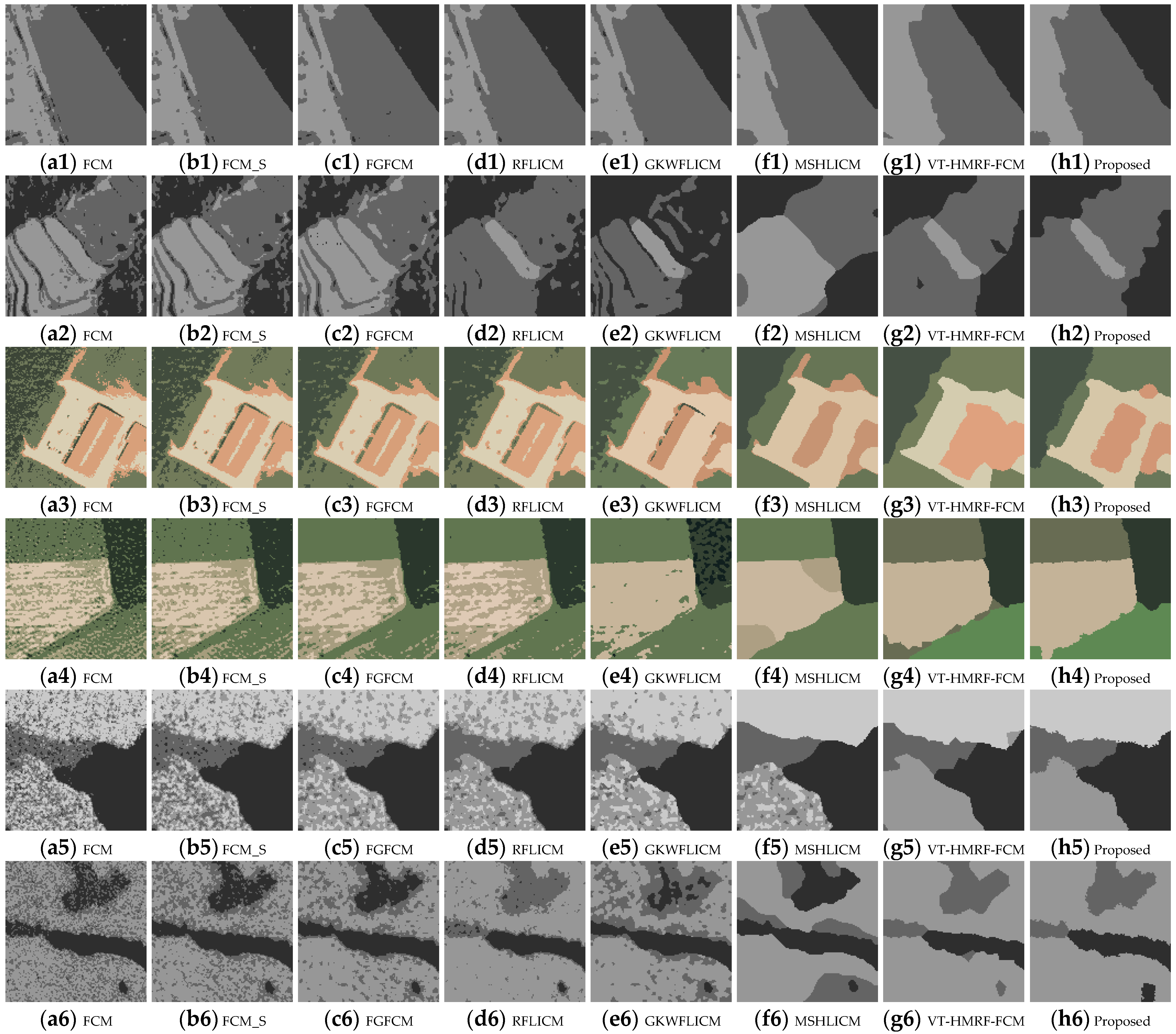
Figure 7 is the classification result of remote sensing images, where each column represents algorithms FCM, FCM_S, FGFCM, RFLICM, GKWFLICM, MSHLICM, VT-HMRF-FCM, and the proposed FVT-FCM. It shows that the four pixel-based algorithms, FCM, FCM_S, FGFCM, and RFLICM, have poor noise resistance. Their performance is very close, except for Figure 7(d2). There are a large number of misclassified pixels in the result. GKWFLICM has a certain degree of noise resistance, but it has poor ability in areas with similar colors, as shown in Figure 7(e3,e5). MSHLICM can overcome most of the noise, and the phenomenon of salt and pepper has significantly improved. But, the classification performance is extremely unstable; the classification results occasionally perform well, as shown in Figure 7(f1,f3), and occasionally perform poorly, as shown in Figure 7(f2,f4,f6). VT-HMRF-FCM, as a region-based classification algorithm, has demonstrated strong noise resistance. However, it is difficult to classify details and boundaries effectively because of the rigidity of polygons, as shown in Figure 7(g3,g4). The proposed algorithm FVT-FCM effectively compensates for VT-HMRF-FCM’s shortcomings through a hierarchical fuzzy membership model. It flexibly achieves accurate boundary classification while ensuring noise resistance, as shown in Figure 7(h1–h6).

Figure 7. Classification results of remote sensing images.

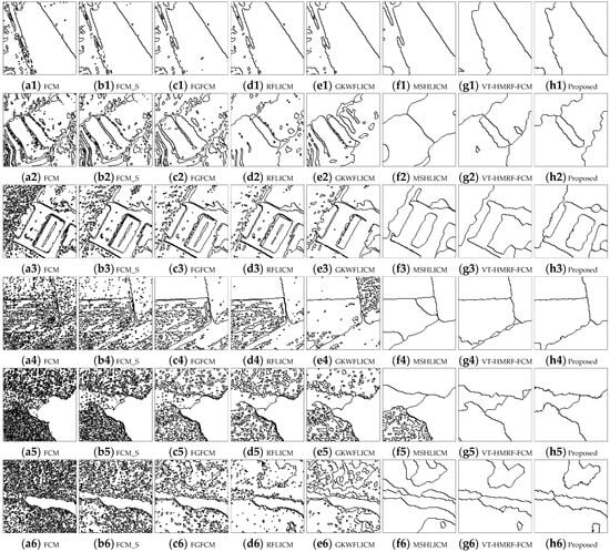
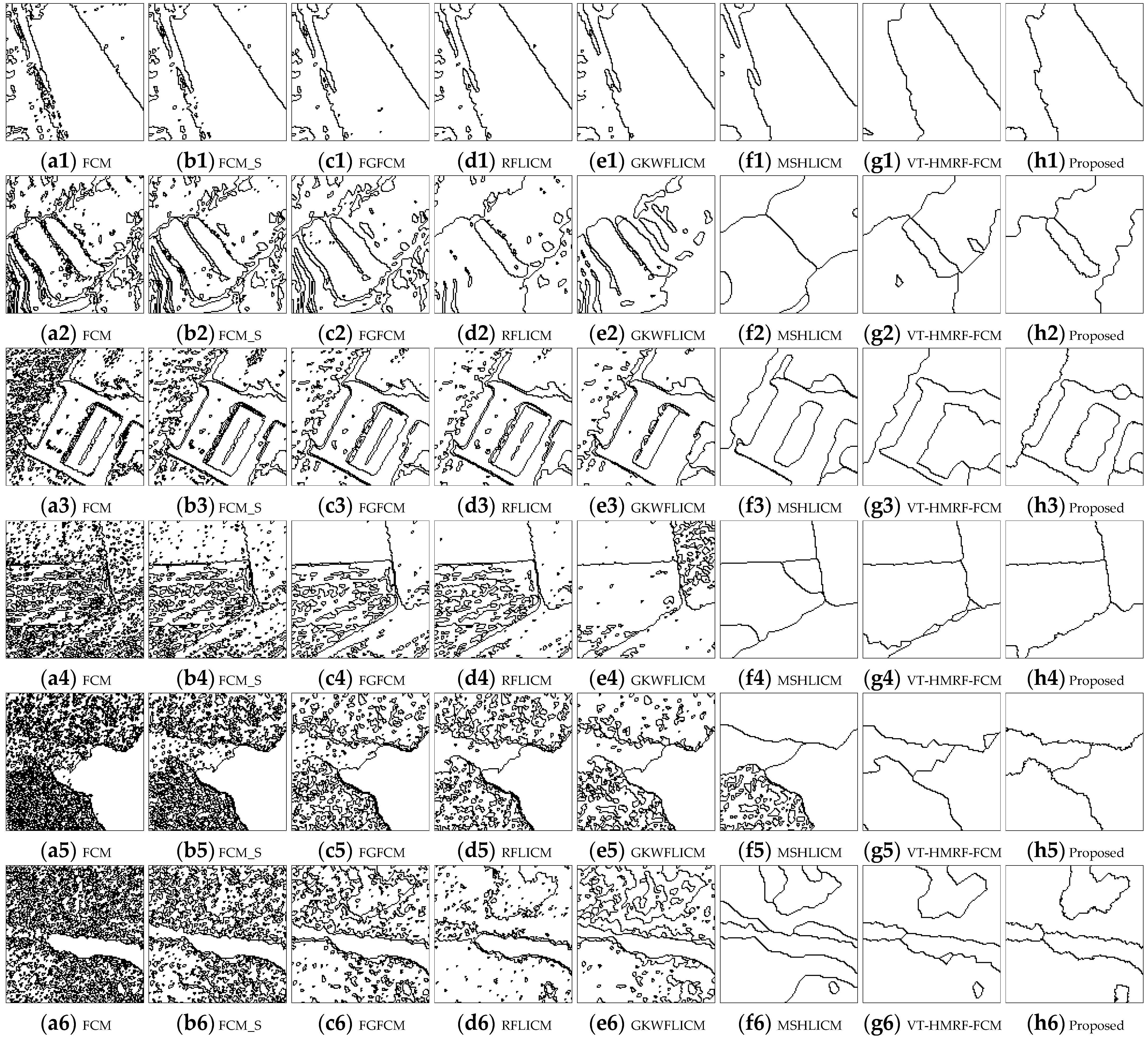
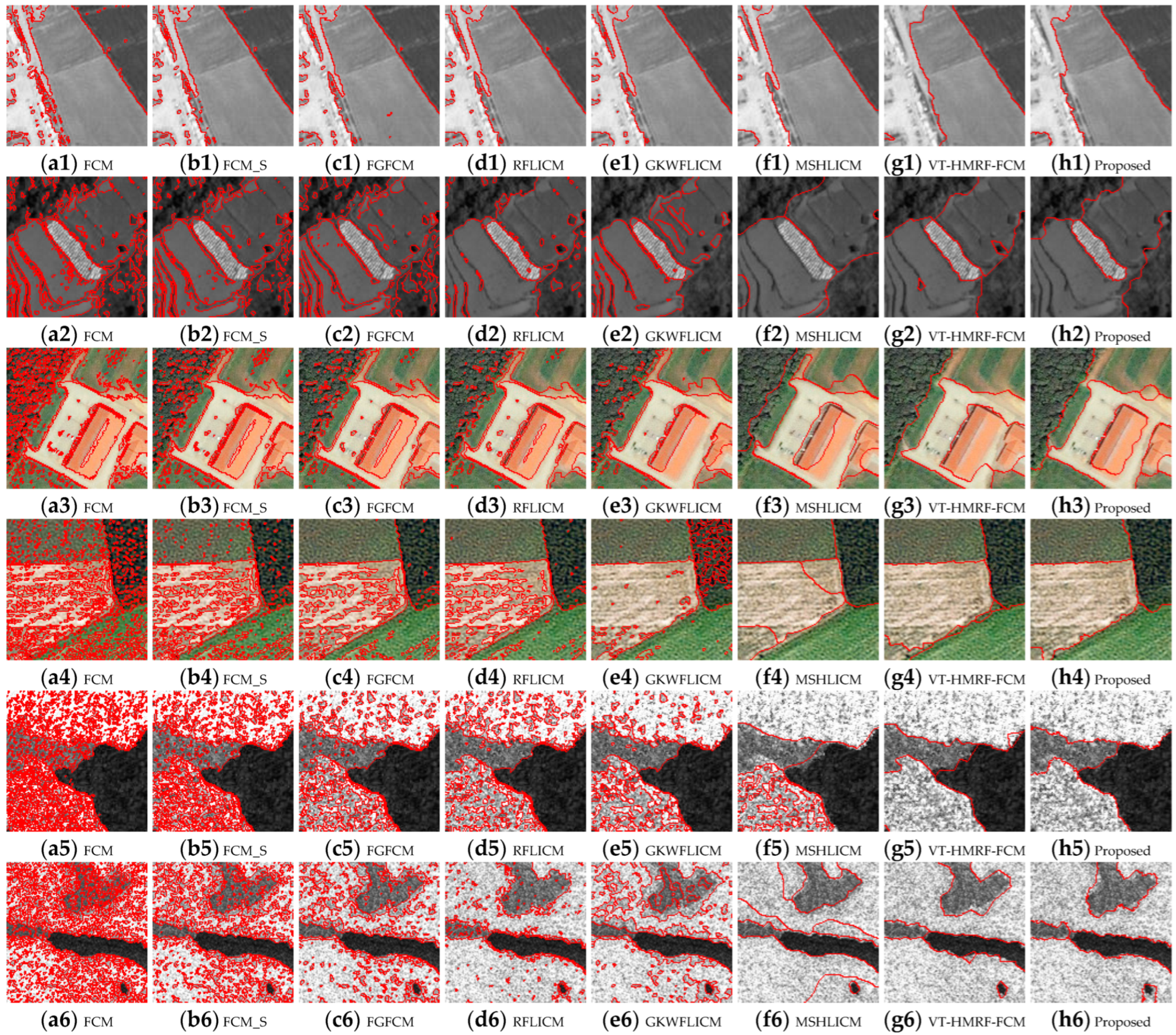
Figure 8 is the contour line images of remote sensing image classification results, where each column represents algorithms FCM, FCM_S, FGFCM, RFLICM, GKWFLICM, MSHLICM, VT-HMRF-FCM, and the proposed FVT-FCM. The content of contour lines can reflect the number of misclassified pixels. It can be seen that FCM, FCM_S, FGFCM, RFLICM, and GKWFLICM have the highest contour line content. This indicates that the five algorithms have poor noise immunity. MSHLICM, VT-HMRF-FCM, and the proposed FVT-FCM are similar, but there are still some redundant contour lines at the boundaries in MSHLICM and VT-HMRF-FCM, which indicates that their performance in boundary classification is not satisfactory.

Figure 8. Contour line images of remote sensing image classification results.

Figure 9 shows contour line overlay images of remote sensing image classification results, where each column represents algorithms FCM, FCM_S, FGFCM, RFLICM, GKWFLICM, MSHLICM, VT-HMRF-FCM, and the proposed FVT-FCM. The red line can reflect the fitting effect of the boundary in the classification results. It shows that pixel-based algorithms perform better in fitting boundaries than region-based. In these two region-based algorithms, VT-HMRF-FCM, and the proposed FVT-FCM, the proposed FVT-FCM has a better ability to fit uncertain boundaries than VT-HMRF-FCM, as shown in Figure 9(h1–h6).

Figure 9. Contour line overlay images of remote sensing image classification results.

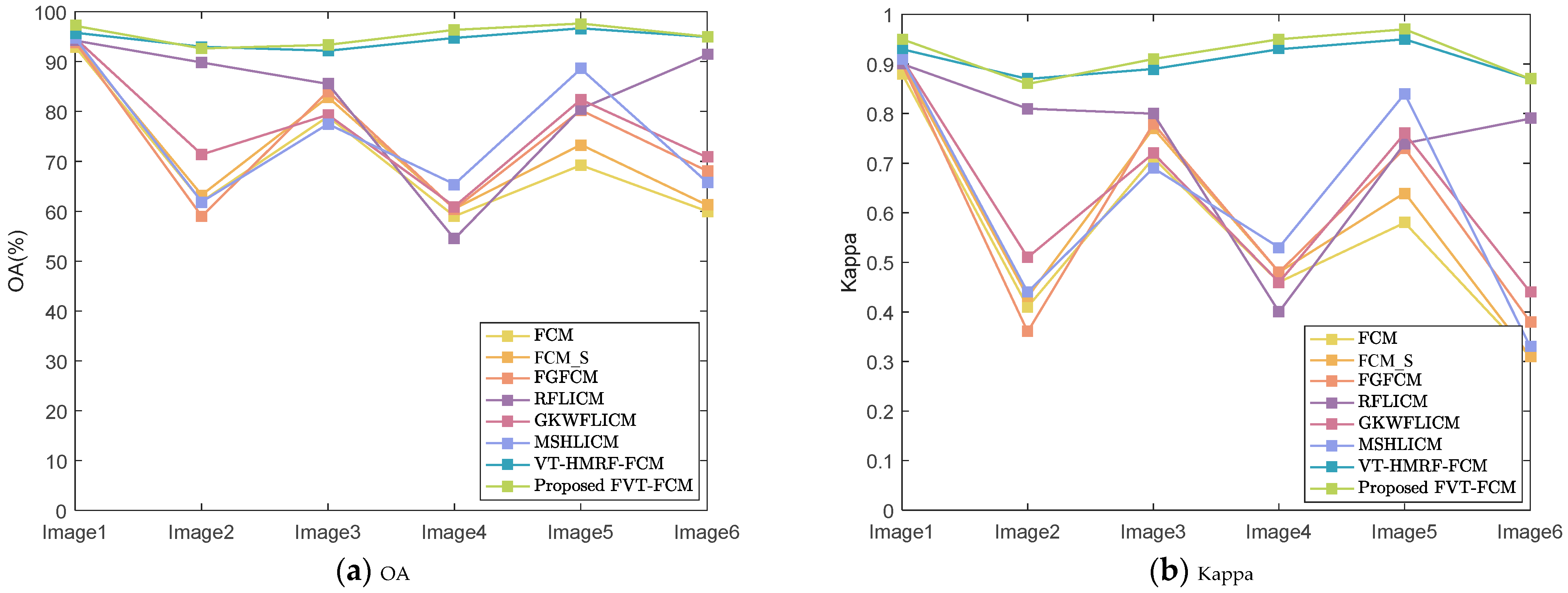
Table 5 shows the quantitative evaluation of the remote sensing image classification results; the accuracy comparison of each image is also shown in Figure 10. It can be seen that Kappa’s trend is the same as that of OA. For OA, pixel-based algorithms are sensitive to different images. For complex images with texture features, similar colors, and strong noise, the OA of pixel-based algorithms can be as low as 50%, Kappa is around 0.4. In contrast, the accuracy of region-based methods is generally stable at a high level, exceeding 90%. The proposed method with a simple model can achieve or even outperform the accuracy of the VT-HMRF-FCM with a complex model.

Table 5. Quantitative evaluation of remote sensing image classification results.

Algorithms	Image 1		Image 2		Image 3		Image 4		Image 5		Image 6
	OA	Ka	OA	Ka	OA	Ka	OA	Ka	OA	Ka	OA	Ka
FCM	92.96	0.88	61.97	0.41	79.01	0.71	58.99	0.46	69.23	0.58	60.02	0.31
FCM_S	93.88	0.90	63.28	0.43	82.87	0.77	60.50	0.48	73.36	0.64	61.22	0.31
FGFCM	93.90	0.90	58.99	0.36	84.04	0.78	60.48	0.48	80.28	0.73	68.09	0.38
RFLICM	94.24	0.90	89.83	0.81	85.54	0.80	54.47	0.40	80.57	0.74	91.37	0.79
GKWFLICM	94.69	0.91	71.37	0.51	79.33	0.72	60.97	0.46	82.40	0.76	70.82	0.44
MSHLICM	94.68	0.91	61.88	0.44	77.49	0.69	65.42	0.53	88.57	0.84	65.80	0.33
VT-HMRF-FCM	95.79	0.93	92.98	0.87	92.19	0.89	94.77	0.93	96.69	0.95	94.96	0.87
Proposed FVT-FCM	97.20	0.95	92.64	0.86	93.38	0.91	96.37	0.95	97.63	0.97	95.05	0.87

Figure 10. Accuracy curves of comparing algorithms and the proposed algorithm; (a) OA, (b) Kappa.

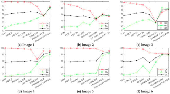
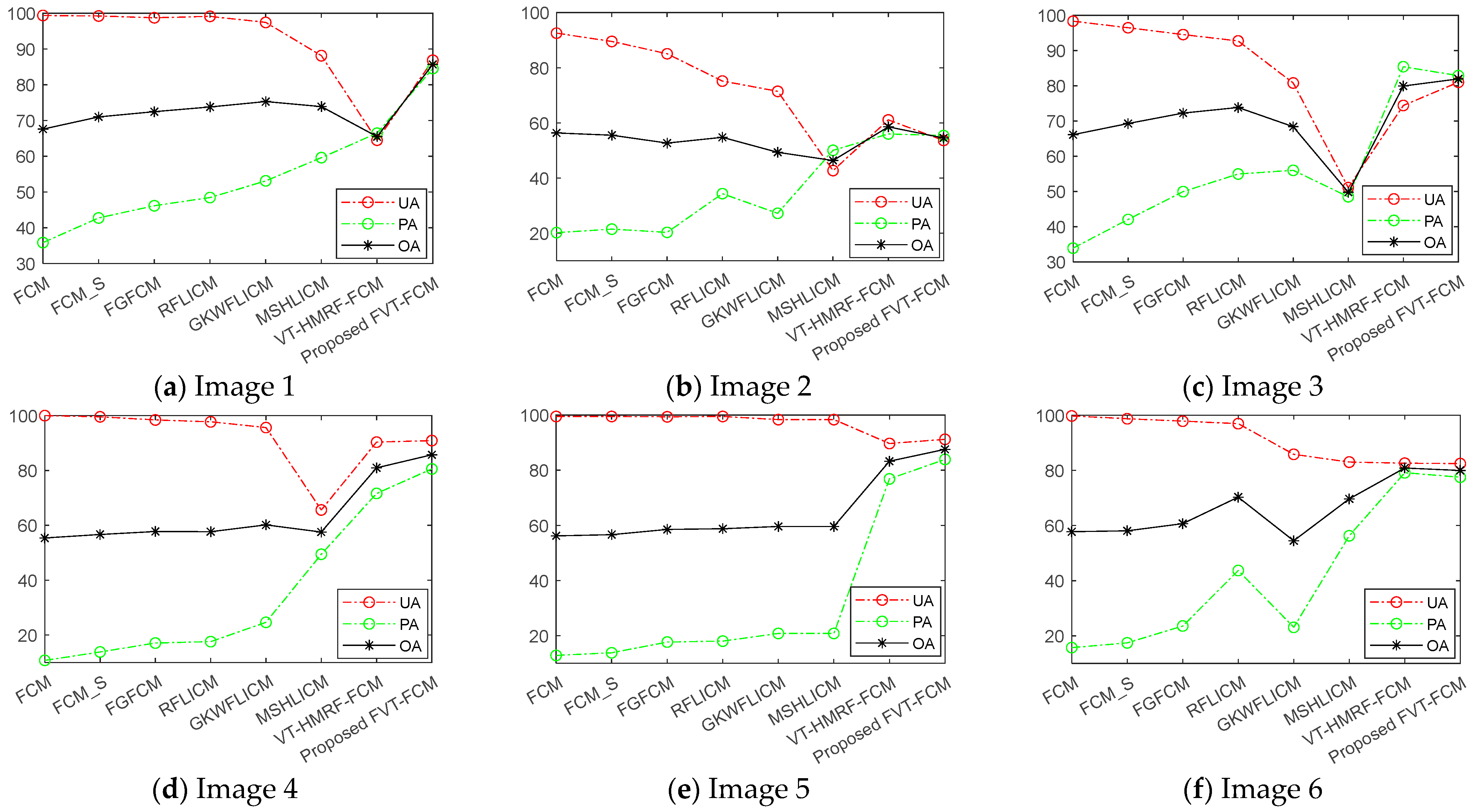
Table 6 shows the boundary accuracy of the remote sensing image classification results, and the comparison of boundary accuracy trends of various algorithms is shown in Figure 11. Figure 11a–f represents image1–6, respectively. As PA increases, UA generally shows a downward trend. When PA and UA are in equilibrium, OA reaches the maximum value. Normally, the UA and PA of VT-HMRF-FCM and the proposed algorithm can balance at a relatively high value. Thus, their OA is higher than other pixel-based algorithms. The proposed method adopts a hierarchical fuzzy membership model, which can further accurately describe boundary effects. Thus, it has higher boundary accuracy, as shown in Figure 11.

Table 6. Boundary accuracy of remote sensing image classification results.

Algorithms	Image 1			Image 2			Image 3			Image 4			Image 5			Image 6
	UA	PA	OA	UA	PA	OA	UA	PA	OA	UA	PA	OA	UA	PA	OA	UA	PA	OA
FCM	99.35	35.85	67.60	92.54	20.22	56.38	98.34	33.94	66.14	100	10.77	55.39	99.50	12.89	56.20	99.77	15.72	57.75
FCM_S	99.22	42.75	70.99	89.55	21.50	55.53	96.47	42.08	69.28	99.58	13.84	56.71	99.50	13.85	56.68	98.75	17.47	58.11
FGFCM	98.71	46.17	72.44	85.07	20.31	52.69	94.54	49.98	72.26	98.46	17.11	57.79	99.38	17.72	58.55	97.88	23.56	60.72
RFLICM	99.10	48.44	73.77	75.18	34.35	54.77	92.72	54.98	73.85	97.76	17.62	57.69	99.50	18.08	58.79	96.95	43.70	70.33
GKWFLICM	97.42	53.10	75.26	71.46	27.23	49.35	80.79	56.02	68.41	95.67	24.65	60.16	98.38	20.85	59.62	85.84	23.11	54.48
MSHLICM	88.11	59.60	73.86	42.72	50.05	46.39	51.10	48.51	49.81	65.64	49.47	57.56	98.38	20.85	59.62	83.02	56.30	69.66
VT-HMRF-FCM	64.47	66.45	65.46	61.10	56.00	58.55	74.42	85.42	79.92	90.36	71.64	81.00	89.70	76.88	83.29	82.62	79.16	80.89
Proposed FVT-FCM	86.82	84.52	85.67	53.64	55.4	54.52	81.00	82.88	81.94	90.92	80.59	85.76	91.19	83.93	87.56	82.47	77.54	80.01

Figure 11. Boundary accuracy curves of various algorithms; (a–f) images 1–6.

5. Discussion

To analyze the performance of the proposed method in depth, the parameter influence, robustness, time complexity, and remaining challenges are discussed in this section.

5.1. Parameter Influence Analysis

In the proposed FVT-FCM, there are six parameters that need to be initialized; they are the number of classes k, the number of polygons m, the regulatory factor q and R, and the fuzzy factors λ₁ and λ₂. k is fixed based on the image. q and R are two regulatory parameters generated from η. q is generally fixed at a smaller value of 0.1. Thus, R plays a major role. For the fuzzy factors, it is generally assumed that λ₁ = λ₂ = λ to simplify the algorithm. Therefore, the main parameters that need to be discussed are m, R, and λ.

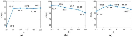
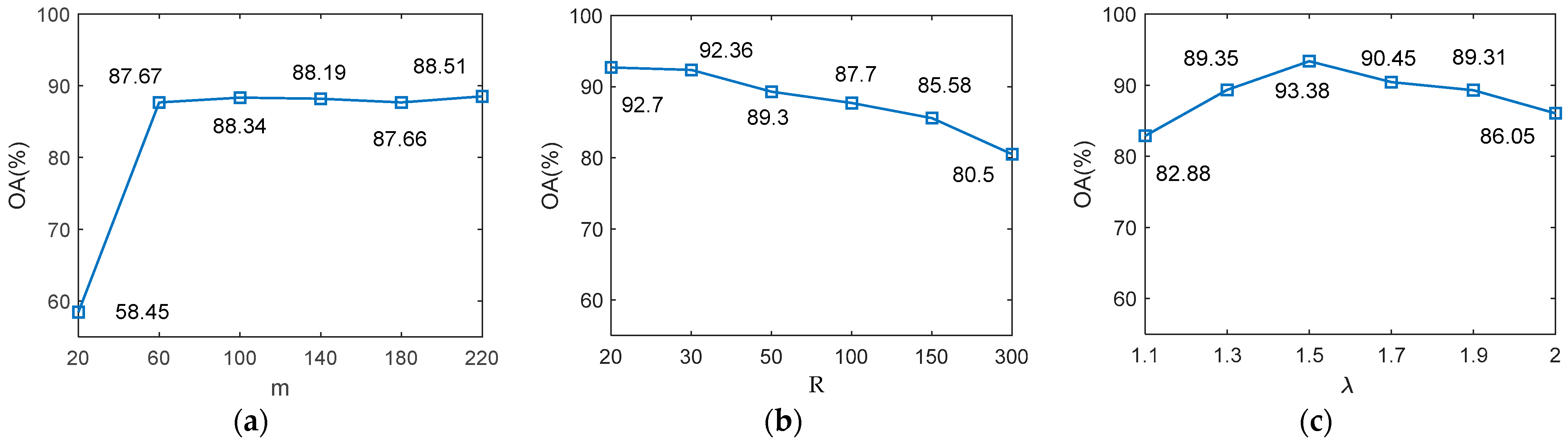
Taking Figure 6(c1) as an example, the curve of classification accuracy with parameter variation is drawn in Figure 12. It can be seen that the impact of parameter m on OA is relatively small when it is greater than 60. For R, OA will slightly decrease as it increases. The main reason is that the higher R will lead to strong local spatial constraints. When R is large enough, the role of Voronoi tessellation in the proposed algorithm is equivalent to that of the VT-HMRF-FCM algorithm. Therefore, the proposed algorithm can be regarded as a general form of the VT-HMRF-FCM algorithm. Normally, the range of values for R is 20–100. For general images, such as panchromatic and multispectral, R ≈ 30. For images with strong noise, such as SAR, R ≈ 100. For λ, OA shows a trend of first increasing and then decreasing with its increase. It indicates that a higher fuzzy degree is not always better, but rather, it should be at a suitable value. A smaller λ is beneficial for distinguishing targets with similar spectra, while a larger λ is beneficial for improving noise resistance. Overall, the recommended range of λ is 1.5–2.5.

Figure 12. Curve of classification accuracy with parameter variation; (a) m, (b) R, (c) λ.

5.2. Robustness Analysis

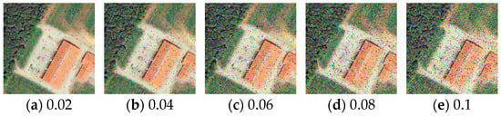
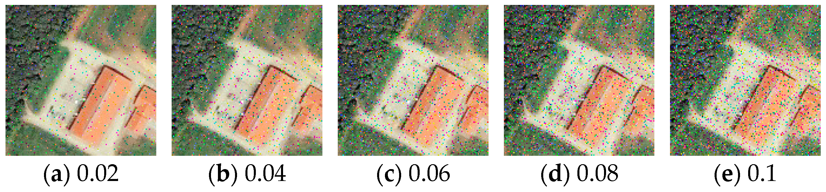
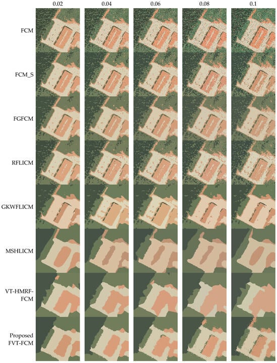
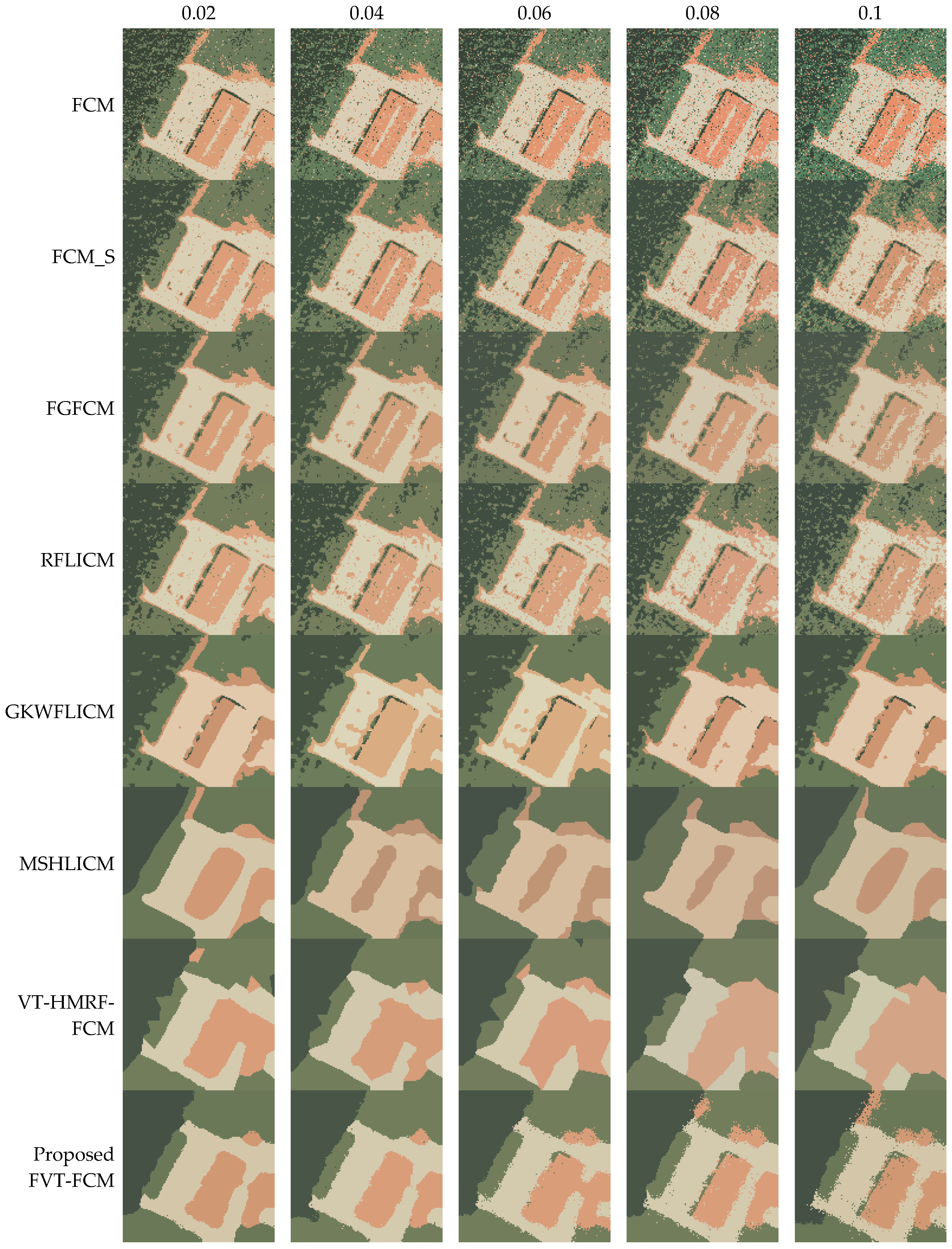
To further demonstrate the classification performance and anti-noise robustness of the proposed algorithm, taking Figure 6(c1) as an example, images with different proportions of salt and pepper noise are generated and tested, as shown in Figure 13 and Figure 14. In Figure 13a–e, their noise ratios are 0.02, 0.04, 0.06, 0.08, and 0.1. Figure 14 shows their classification results. As the proportion of noise increases, the noise in the classification results of the FCM, FCM_S, FGFCM, and RFLICM algorithms also increases. Due to the influence of noise, GKWFLICM and MSHLICM easily get stuck in local optima. Thus, the classification results are extremely unstable. For VT-HMRF-FCM, its boundaries will become rough with the increase in noise, until it is difficult to distinguish small objects. For the proposed algorithm, the classification effect is almost unaffected when the noise is less than 0.06. When it is greater than 0.06, even if there are some misclassifications in the boundary, the classification performance is still better than other algorithms.

Figure 13. Images with different proportions of salt and pepper noise.

Figure 14. Classification results of images with noise.

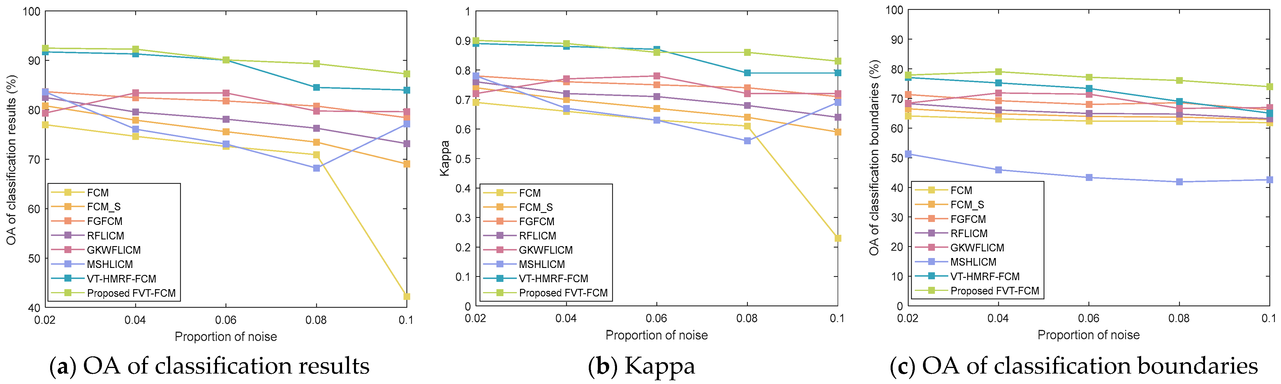
Table 7 shows the quantitative evaluation of classification results, where OA_r represents the OA index of classification results, and OA_b represents the OA index of boundaries. Their changes are visualized in Figure 15. As the proportion of noise increases, each of the accuracy indicators decrease to varying degrees. Among them, FCM has the highest descent speed. GKWFLICM and MSHLICM have extremely unstable accuracy. The accuracy of VT-HMRF-FCM and the proposed FVT-FCM have always been at a high level. Especially when the noise is greater than 0.08, the proposed algorithm is more stable, as shown in Figure 15a,b. In addition, the OA of boundaries of the proposed algorithm are always greater than VT-HMRF-FCM, as shown in Figure 15c.

Table 7. Quantitative evaluation of classification results of images with noise.

Algorithms	0.02			0.04			0.06			0.08			0.1
	OAr	Ka	OAb	OAr	Ka	OAb	OAr	Ka	OAb	OAr	Ka	OAb	OAr	Ka	OAb
FCM	76.99	0.69	64.10	74.62	0.66	63.13	72.61	0.63	62.39	70.91	0.61	62.29	42.21	0.23	61.85
FCM_S	80.82	0.74	66.50	77.89	0.70	64.84	75.57	0.67	63.95	73.44	0.64	63.69	69.05	0.59	62.88
FGFCM	83.66	0.78	71.29	82.46	0.76	69.23	81.78	0.75	67.95	80.76	0.74	68.57	78.40	0.71	66.15
RFLICM	82.50	0.76	68.27	79.55	0.72	66.10	78.09	0.71	64.92	76.27	0.68	64.73	73.16	0.64	63.17
GKWFLICM	79.35	0.72	68.42	83.44	0.77	71.87	83.40	0.78	71.45	79.75	0.72	66.66	79.61	0.72	66.94
MSHLICM	83.61	0.78	51.25	76.06	0.67	45.94	73.07	0.63	43.30	68.21	0.56	41.83	77.13	0.69	42.58
VT-HMRF-FCM	91.69	0.89	77.06	91.30	0.88	75.23	90.04	0.87	73.35	84.53	0.79	68.99	83.98	0.79	65.00
Proposed FVT-FCM	92.46	0.90	77.90	92.27	0.89	79.00	90.07	0.86	77.14	89.33	0.86	76.06	87.26	0.83	73.95

Figure 15. Accuracy curve with the change in noise proportion.

5.3. Time Complexity Analysis

To verify the time efficiency of the proposed FVT-FCM algorithm, the execution times of the remote sensing images are listed in Table 8. It can be seen that the time complexity of multispectral images (Images 3 and 4) with three bands is significantly higher than that of panchromatic images (Images 1 and 2) and SAR images (Images 5 and 6) with one band. In the six pixel-based comparing algorithms, all other algorithms have lower time complexity except for MSHLICM. The main reason for the high time complexity of MSHLICM is that it needs to calculate the second-level neighborhood based on the first-level neighborhood. The time complexity of VT-HMRF-FCM ranks second because it needs to seek the optimal solution for seed points through random sampling. The proposed algorithm is not as fast as the first five algorithms. The main reason is that the proposed FVT-FCM is region-based. Nonetheless, its execution time is superior to both the region-based algorithm VT-HMRF-FCM and pixel-based algorithm MSHLICM. Based on the comprehensive analysis of classification accuracy and execution time, the proposed method can be regarded as the most optimal one.

Table 8. Execution time of different algorithms in remote sensing images; (sec).

Algorithms	Images
	Image 1	Image 2	Image 3	Image 4	Image 5	Image 6
FCM	1.11	1.28	1.72	4.84	2.21	7.61
FCM_S	0.04	0.04	0.04	0.20	0.06	0.08
FGFCM	0.04	0.04	0.13	0.13	0.03	0.07
RFLICM	0.13	0.24	0.19	0.85	0.12	0.29
GKWFLICM	2.94	8.16	9.09	5.97	0.42	1.87
MSHLICM	3724.40	6032.45	16,026.48	17,318.53	6080.06	4792.17
VT-HMRF-FCM	316.56	326.59	1386.42	1042.08	627.88	574.41
Proposed FVT-FCM	198.37	220.23	623.47	687.90	343.45	226.73

To understand its universality, the time complexity will be further analyzed from the perspective of the model mechanism. It is mainly related to the following factors: the number of pixels n, the number of clusters k, the number of gray levels N_ɩ, the size of the neighborhood window e, and the number of iterations t. Then, the time complexities of all algorithms in this paper are given in Table 9. It can be seen that FCM_S and GKWFLICM have an additional neighborhood term e compared to FCM. In FGFCM, N_ɩ << n. Therefore, it is fast. RFLICM needs to calculate the local coefficient of variation based on the neighborhood, thus its time complexity is O(ne + nket). In MSHLICM, the second layer neighborhood needs to be calculated based on the first layer neighborhood, so the algorithm complexity is extremely high. In the region-based algorithm, polygons have replaced the neighborhood and become a spatial constraint term, thus m is also an important factor. Although the time complexity of VT-HMRF-FCM and the proposed algorithm is O(nmkt), VT-HMRF-FCM needs a large t to find the optimal solution. Therefore, its time complexity is higher than the proposed.

Table 9. Execution time of different algorithms in remote sensing images; (sec).

Algorithms	Time Complexity	Algorithms	Time Complexity
FCM	O(nkt)	GKWFLICM	O(nket)
FCM_S	O(nket)	MSHLICM	O(nket + nke2t)
FGFCM	O(Nɩkt)	VT-HMRF-FCM	O(nmkt)
RFLICM	O(ne + nket)	Proposed FVT-FCM	O(nmkt)

5.4. Remaining Challenges

The effectiveness and robustness of the proposed algorithm have been effectively demonstrated in previous experiments and discussions. This provides a new way for unsupervised classification that can balance noise resistance and boundary fitting. However, it still faces many challenges, such as the following: (1) How to extend its application to large regions. Due to the direct correlation between time complexity and pixel count, large region images inevitably bring more computation time and memory. Thus, we recommend clipping the large image into a series of small images first, and then combining parallel computing for classification. It can maintain classification accuracy while ensuring classification efficiency. (2) How to better distinguish targets with complex scenes. At present, only spectral and spatial information are used in this paper. It can achieve better classification of most general images. To better describe complex scenes, texture information, contextual information, semantic information, etc., will be further considered to establish model constraints.

6. Conclusions

In this paper, an unsupervised image classification algorithm based on fully fuzzy Voronoi tessellation is proposed. It innovatively describes a new fundamental unit, i.e., fuzzy polygons. Based on fuzzy polygons, a hierarchical fuzzy membership model is established to explore the uncertainty in the classification process. The first level models the uncertainty of pixels and fuzzy polygons, while the second level models the uncertainty between fuzzy polygons and categories by considering the transitivity of fuzzy. Its main advantage is that it has both the noise resistance of region-based algorithms and the flexibility and strong boundary fitting of pixel-based algorithms. Additionally, Voronoi tessellation is explicitly modeled in the objective function, which facilitates optimization of Voronoi tessellation through analytical solutions rather than random sampling methods used previously, which can accelerate algorithm convergence. The proposed algorithm explores the feasibility and effectiveness of fuzzy polygons in image classification. In the future, the classification method based on fuzzy polygon-level spatial constraints and multifeatures will be proposed to further enhance the classification accuracy of complex images.

References

- Chen, H.; Long, H.; Chen, T.; Song, Y.; Chen, H.; Zhou, X.; Deng, W. M³FuNet: An Unsupervised Multivariate Feature Fusion Network for Hyperspectral Image Classification. IEEE Trans. Geosci. Remote Sens. 2024, 62, 5513015. [Google Scholar] [CrossRef] [Scilit]
- Yang, S.; Zhang, J.; Wang, J.; Zhang, S.; Bai, Y.; Shi, S.; Cao, D. Spatiotemporal variations of water productivity for cropland and driving factors over China during 2001–2015. Agric. Water Manag. 2022, 262, 107328. [Google Scholar] [CrossRef] [Scilit]
- Shelhamer, E.; Long, J.; Darrell, T. Fully Convolutional Networks for Semantic Segmentation. IEEE Trans. Pattern Anal. Mach. Intell. 2017, 39, 640–654. [Google Scholar] [CrossRef] [Scilit] [PubMed]
- Lee, H.; Kwon, H. Going Deeper With Contextual CNN for Hyperspectral Image Classification. IEEE Trans. Image Process. 2017, 26, 4843–4855. [Google Scholar] [CrossRef] [Scilit] [PubMed]
- Ronneberger, O.; Fischer, P.; Brox, T. U-Net: Convolutional Networks for Biomedical Image Segmentation. In Proceedings of the 18th International Conference on Medical Image Computing and Computer-Assisted Intervention (MICCAI), Munich, Germany, 5–9 October 2015. [Google Scholar]
- Zhou, Z.; Siddiquee, M.M.R.; Tajbakhsh, N.; Liang, J. UNet++: Redesigning Skip Connections to Exploit Multiscale Features in Image Segmentation. IEEE Trans. Med. Imaging 2020, 39, 1856–1867. [Google Scholar] [CrossRef] [Scilit] [PubMed]
- Chen, L.C.; Papandreou, G.; Kokkinos, I.; Murphy, K.; Yuille, A.L. DeepLab: Semantic Image Segmentation With Deep Convolutional Nets, Atrous Convolution, and Fully Connected CRFs. IEEE Trans. Pattern Anal. Mach. Intell. 2018, 40, 834–848. [Google Scholar] [CrossRef] [Scilit]
- Chen, L.; Papandreou, G.; Schroff, F.; Adam, H. Rethinking Atrous Convolution for Semantic Image Segmentation. arXiv 2017, arXiv:1706.05587. [Google Scholar]
- Chen, L.C.; Zhu, Y.; Papandreou, G.; Schroff, F.; Adam, H. Encoder-Decoder with Atrous Separable Convolution for Semantic Image Segmentation. In Proceedings of the European Conference on Computer Vision (ECCV), Munich, Germany, 8–14 September 2018. [Google Scholar]
- Xia, G.S.; Hu, J.; Hu, F.; Shi, B.; Bai, X.; Zhong, Y.; Liu, D.; Zhang, L. Remote Sensing Image Scene Classification: Benchmark and State of the Art. Proc. IEEE 2017, 105, 1865–1883. [Google Scholar]
- Caron, M.; Bojanowski, P.; Joulin, A.; Douze, M. Deep Clustering for Unsupervised Learning of Visual Features. In Proceedings of the European Conference on Computer Vision (ECCV), Munich, Germany, 8–14 September 2018. [Google Scholar]
- Asano, Y.M.; Rupprecht, C.; Vedaldi, A. Self-labelling via simultaneous clustering and representation learning. In Proceedings of the International Conference on Learning Representations (ICLR), Addis Ababa, Ethiopia, 26–30 April 2020. [Google Scholar]
- Hung, C.C.; Kulkarni, S.; Kuo, B.C. A New Weighted Fuzzy C-Means Clustering Algorithm for Remotely Sensed Image Classification. IEEE J. Sel. Top. Signal Process. 2011, 5, 543–553. [Google Scholar] [CrossRef] [Scilit]
- Lei, T.; Jia, X.; Zhang, Y.; Liu, S.; Meng, H.; Nandi, A.K. Superpixel-Based Fast Fuzzy C-Means Clustering for Color Image Segmentation. IEEE Trans. Fuzzy Syst. 2019, 27, 1753–1766. [Google Scholar] [CrossRef] [Scilit]
- Zhao, F.; Tian, M.; Xie, W.; Liu, H. A New Parallel Dual-Channel Fully Convolutional Network Via Semi-Supervised FCM for PolSAR Image Classification. IEEE J. Sel. Top. Appl. Earth Obs. Remote Sens. 2020, 13, 4493–4505. [Google Scholar] [CrossRef] [Scilit]
- Song, J.; Li, Y.; Li, X.; Yang, S.; Xie, J.; Zhu, R. Unsupervised remote sensing image classification with differentiable feature clustering by coupled transformer. J. Appl. Remote Sens. 2024, 18, 026505. [Google Scholar] [CrossRef] [Scilit]
- Wang, Y.; Gu, M. Classification methods for hyperspectral remote sensing images with weak texture features. J. Radiat. Res. Appl. Sci. 2024, 17, 101019. [Google Scholar] [CrossRef] [Scilit]
- Lu, Y.; Li, H.; Zhang, C.; Zhang, S. Object-Based Semi-Supervised Spatial Attention Residual UNet for Urban High-Resolution Remote Sensing Image Classification. Remote Sens. 2024, 16, 1444. [Google Scholar] [CrossRef] [Scilit]
- Wang, Q.; Miao, Y.; Chen, M.; Yuan, Y. Spatial-Spectral Clustering With Anchor Graph for Hyperspectral Image. IEEE Trans. Geosci. Remote Sens. 2022, 60, 5542413. [Google Scholar] [CrossRef] [Scilit]
- Ahmed, M.N.; Yamany, S.M.; Mohamed, N.; Farag, A.A.; Moriarty, T. A modified fuzzy C-means algorithm for bias field estimation and segmentation of MRI data. IEEE Trans. Med. Imaging 2002, 21, 193–199. [Google Scholar] [CrossRef] [Scilit]
- Chen, S.; Zhang, D. Robust image segmentation using FCM with spatial constraints based on new kernel-induced distance measure. IEEE Trans. Syst. Man Cybern. 2004, 34, 1907–1916. [Google Scholar] [CrossRef] [Scilit]
- Szilagyi, L.; Benyo, Z.; Szilagyi, S.; Adam, H. MR brain image segmentation using an enhanced fuzzy C-means algorithm. In Proceedings of the 25th Annual International Conference of the IEEE Engineering in Medicine and Biology Society, Cancun, Mexico, 17–21 September 2003. [Google Scholar]
- Cai, W.; Chen, S.; Zhang, D. Fast and robust fuzzy C-means clustering algorithms incorporating local information for image segmentation. Pattern Recognit. 2007, 40, 825–838. [Google Scholar] [CrossRef] [Scilit]
- Krinidis, S.; Chatzis, V. A robust fuzzy local information C-means clustering algorithm. IEEE Trans. Image Process. 2010, 19, 1328–1337. [Google Scholar] [CrossRef] [Scilit]
- Gong, M.; Zhou, Z.; Ma, J. Change detection in synthetic aperture radar images based on image fusion and fuzzy clustering. IEEE Trans. Image Process. 2012, 21, 2141–2151. [Google Scholar] [CrossRef] [Scilit]
- Gong, M.; Liang, Y.; Shi, J.; Ma, W.; Ma, J. Fuzzy C-means clustering with local information and kernel metric for image segmentation. IEEE Trans. Image Process. 2013, 22, 573–584. [Google Scholar] [CrossRef] [Scilit] [PubMed]
- Memon, K.H.; Lee, D. Generalised kernel weighted fuzzy C-means clustering algorithm with local information. Fuzzy Set. Syst. 2018, 340, 91–108. [Google Scholar] [CrossRef] [Scilit]
- Zhang, X.; Sun, Y.; Liu, H.; Hou, Z.; Zhao, F.; Zhang, C. Improved clustering algorithms for image segmentation based on non-local information and back projection. Inf. Sci. 2020, 550, 129–144. [Google Scholar] [CrossRef] [Scilit]
- Tang, Y.; Ren, F.; Pedrycz, W. Fuzzy C-means clustering through SSIM and patch for image segmentation. Appl. Soft. Comput. 2020, 87, 105928. [Google Scholar] [CrossRef] [Scilit]
- Wu, C.; Qi, X. Local feature driven fuzzy local information C-means clustering with kernel metric for blurred and noisy image segmentation. J. Real-Time Image Process. 2023, 20, 116. [Google Scholar] [CrossRef] [Scilit]
- Wu, C.; Wu, W. Master-slave hierarchy local information driven fuzzy C-means clustering for noisy image segmentation. Visual Comput. 2024, 40, 865–897. [Google Scholar] [CrossRef] [Scilit]
- Zhao, Q.; Li, X.; Li, Y.; Zhao, X. A fuzzy clustering image segmentation algorithm based on Hidden Markov Random Field models and Voronoi Tessellation. Pattern Recogn. Lett. 2017, 85, 49–55. [Google Scholar] [CrossRef] [Scilit]
- Chatzis, S.P.; Varvarigou, T.A. A fuzzy clustering approach toward hidden Markov random field models for enhanced spatially constrained image segmentation. IEEE Trans. Fuzzy Syst. 2008, 16, 1351–1361. [Google Scholar] [CrossRef] [Scilit]
- Li, X.; Chen, J.; Zhao, L.; Guo, S.; Sun, L.; Zhao, X. Adaptive Distance-Weighted Voronoi Tessellation for Remote Sensing Image Segmentation. Remote Sens. 2020, 12, 4115. [Google Scholar] [CrossRef] [Scilit]
Disclaimer/Publisher’s Note: The statements, opinions and data contained in all publications are solely those of the individual author(s) and contributor(s) and not of MDPI and/or the editor(s). MDPI and/or the editor(s) disclaim responsibility for any injury to people or property resulting from any ideas, methods, instructions or products referred to in the content. |
© 2024 by the authors. Licensee MDPI, Basel, Switzerland. This article is an open access article distributed under the terms and conditions of the Creative Commons Attribution (CC BY) license (https://creativecommons.org/licenses/by/4.0/).