


Abstract
In this study, we introduce a novel self-adaptive alternating direction method of multipliers tailored for image denoising. Our approach begins by formulating a collaborative regularization model that upholds structured sparsity within images while delving into spatial correlations among pixels. To address the challenge of penalty parameter influence on convergence speed, we innovate by proposing a self-adaptive alternating direction method of multipliers. This adaptive technique autonomously adjusts variable penalty parameters to expedite algorithm convergence, thereby markedly boosting algorithmic performance. Through a fusion of simulations and empirical analyses, our research demonstrates that this novel methodology significantly amplifies the efficacy of denoising processes.
1. Introduction
Image denoising occupies a pivotal role within the realm of digital image processing, functioning as a foundational task crucial for refining and accentuating the intrinsic qualities inherent in an image [1,2,3,4]. Noise, stemming from a multitude of sources, such as image acquisition devices, transmission channels, or storage modalities, presents a substantial impediment to maintaining image fidelity. The presence of noise can obfuscate intricate details, introduce artifacts, and degrade the overall visual fidelity of an image. Through the efficacious elimination of noise via denoising methodologies, the quality, integrity, and interpretability of images can be significantly augmented [5,6,7,8]. In domains like medical imaging, surveillance, remote sensing, and scientific inquiry, where accurate and lucid visual information holds paramount importance, the indispensability of image denoising cannot be overstated. It not only enhances the aesthetic allure of images but also safeguards the preservation of critical details, fostering more dependable analysis, interpretation, and decision-making grounded in visual data [9,10,11].
Common image denoising techniques include statistical modeling, transformation methods, and deep learning strategies [12,13,14]. Compared to other methods, transformation methods have efficient algorithm implementations, capable of processing large-scale data in a short time. They also exhibit good adaptability to various signal types, making them suitable for a variety of image processing tasks. Low-rank matrix recovery techniques model low-rank matrices within the image domain to restore the original low-rank structure from corrupted image data [15,16,17,18]. This approach leverages the latent low-rank properties within images, representing the image as a sum of a low-rank matrix capturing structural information and a sparse matrix representing noise and fine details. Through low-rank matrix recovery techniques, noise in images can be removed while preserving essential structural features, resulting in clearer and more accurate image restoration [19].
Low-rank matrix recovery techniques include singular value soft thresholding, low-rank nuclear norm regularization, alternating direction method of multipliers, and low-rank representation methods [20,21,22]. These methods operate by manipulating singular values, introducing penalties based on low-rank nuclear norms, employing alternating optimization schemes, or utilizing low-rank representations to restore the low-rank structure of images while eliminating noise. In recent years, several works have garnered significant attention. For example, in [23], Liu et al. utilized sparse signal representation methods and designed overcomplete dictionaries to explore the advantages and limitations of sparse signal representation algorithms in the processing of ultrasonic non-destructive evaluation signals. In [24], Hu et al. reconstructed images from their under-sampled Fourier coefficients using infimal convolution regularizations, and an advanced Generalized Structured Low-Rank Algorithm is introduced. Due to its applicability to various constraints and regularization terms, the ADMM has garnered more attention among these low-rank matrix recovery algorithms.
The traditional ADMM methodology employs the minimization of the (1,1)-norm of a matrix to enforce sparsity and control the count of non-zero elements, thereby approximating the optimization of the matrix’s 0-norm to a certain degree. However, neighboring pixels in images typically exhibit correlations. By enforcing sparse constraints on individual pixels, there is a risk of losing model intricacies and structural nuances. Through the utilization of collaborative sparse regression, a shared sparse representation can be identified, preserving structured sparsity within the image and enabling a deeper analysis of spatial interrelations among pixels [25]. To mitigate the impact of penalty parameters on convergence rates, an adaptive approach based on a balance principle for selecting appropriate penalty parameters is introduced. This methodology, proven effective in projection techniques and Uzawa block relaxation algorithms [26,27], is leveraged in this study to propose a self-adaptive ADMM strategy. This strategy dynamically selects variable penalty parameters to expedite algorithm convergence, markedly enhancing algorithmic efficacy.
This paper aims to enhance denoising effectiveness by introducing a collaborative regularization model and proposing a self-adaptive alternating direction method of multipliers to achieve faster algorithm convergence. The key contributions are as follows:
- Formulate a collaborative regularization model that maintains structured sparsity within images and explores spatial correlations among pixels.
- Propose a self-adaptive alternating direction method of multipliers to achieve faster algorithm convergence.
The remaining part of this paper is organized as follows. In Section 2, the related works are discussed. In Section 3, low-rank matrix recovery and the alternating direction method of multipliers are introduced. In Section 4, the proposed collaborative regularization model and improved algorithm are proposed. In Section 5, two examples are provided. Finally, some concluding remarks are given in Section 6.
2. Related Work
In recent years, image denoising has become a highly regarded application area in the field of artificial intelligence. In image processing, the Low-Rank Matrix Recovery (LRMR) technique has been successfully applied to remove noise from images, enhancing image quality and clarity [28,29]. LRMR technology extends the concept of sparse representation of sample vectors to the low-rank scenario of matrices, becoming another important method for image denoising, following the path of compressive sensing (CS). In image denoising, LRMR decomposes the image data matrix into the sum of a low-rank matrix and a sparse noise matrix, then restores the low-rank matrix by solving a nuclear norm optimization problem, effectively eliminating noise from the image. Currently, LRMR mainly includes several common models such as Robust Principal Component Analysis (RPCA), Matrix Completion (MC), and Low-Rank Representation (LRR), all of which demonstrate good image denoising effects in various scenarios [30,31].
RPCA is a technique used to handle outlier values and noise in data, aiming to decompose the original data matrix into low-rank and sparse components. The core idea of RPCA assumes that the data matrix consists of a low-rank structure and a sparse noise component, recovering the original data by minimizing the difference between these two parts, thereby achieving denoising and outlier detection. RPCA exhibits strong robustness to outlier values and noise in data, effectively dealing with interfering factors, enhancing data accuracy and stability. It finds wide applications in fields such as image processing, video analysis, signal processing, and more. For example, in [32], Chen et al. proposed a robust PCA method that relies on a nonconvex low-rank approximation and total variational regularization (TV) to address the image denoising problem, aiming to enhance the denoising performance. In [33], Wu et al., proposed a workflow to reduce seismic traffic noise by utilizing the -norm RPCA method. Although these algorithms perform well under specific common scenarios, in order to achieve real-time processing, it is necessary to accelerate and optimize the low-rank matrix recovery algorithm. This optimization involves reducing algorithm complexity, minimizing computational burden, and this is also one of the main insights of our research.
3. Preliminaries and Problem Statement
3.1. Low-Rank Matrix Recovery
The application of low-rank matrix recovery in image denoising is a significant and effective technique within the field of image processing. In the field of image processing, images are often regarded as matrices with low-rank properties due to the inherent correlations and structural information among pixels. The objective of image denoising is to eliminate noise from various sources such as sensor noise, compression artifacts, or communication channel interference to enhance image quality and clarity.
For a given matrix containing noise, the matrix can be decomposed into the sum of two matrices, i.e., , where the matrices and are unknown, but is low-rank. When the elements of the matrix obey an independent identically distributed Gaussian distribution, the classical PCA can be used to obtain the optimal matrix , i.e., to solve the following optimization problem.
When is a sparse large noise matrix, PCA is no longer applicable. In this case, the recovery of the low-rank matrix is a two-objective optimization problem
The bi-objective optimization problem (2) is converted into a single-objective optimization problem by introducing a trade-off factor as follows:
Since the objective function of Equation (3) is non-convex, it can be approximated by the following equation:
Remark 1.
The (1,1)-norm of a matrix is defined as the maximum absolute sum of each column. In a sense, this maximum value can be seen as an upper bound on the number of non-zero elements in the matrix. Therefore, minimizing the (1,1)-norm of a matrix also serves as a constraint on the number of non-zero elements, thus providing an approximation to optimizing the 0-norm of a matrix.
Remark 2.
The problem of solving Equation (4) is known as Robust Principal Component Analysis (RPCA), which provides an efficient way to solve the low-rank matrix recovery problem and can improve robustness to outliers in the data.
Remark 3.
In reference [15], it is pointed out that as long as the singular values distribution of the low-rank matrix is reasonable and the non-zero elements of the sparse matrix are uniformly distributed, the convex optimization problem (4) can recover the original low-rank matrix from any unknown error with a probability close to 1.
3.2. Traditional Alternating Direction Method of Multipliers
The Alternating Direction Method of Multipliers (ADMM) is an iterative algorithm used for solving convex optimization problems. ADMM decomposes the original problem into easier-to-handle subproblems and iteratively solves these subproblems alternately, combined with updating the multipliers to progressively approach the optimal solution of the original problem. This method excels in dealing with problems that have structural constraints and finds wide applications in distributed optimization and machine learning fields. Introducing the augmented Lagrangian function for problem (4):
where is the Lagrange multiplier and is the given penalty parameter. Using the Exact Augmented Lagrangian Method (EALM), alternatively iterate matrices and ,
If and represent the precise values of and , the formula for updating matrix is as follows:
where the updating method for parameter can be found in reference [15].
4. Proposed Model and Improved Algorithm
This section primarily outlines the refinement of our collaborative regularization model [25]. In enhancing the convergence speed while solving this model, we propose our self-adaptive alternating direction method by deriving adaptive step sizes.
4.1. A Collaborative Regularization Model
In image denoising, noise can be seen as high-frequency variations that disrupt the smoothness and continuity of the image. By representing an image as a low-rank matrix (which captures the underlying structure and patterns in the image), the high-frequency noise components can often be separated from the low-rank structure during the denoising process. Images often exhibit high levels of redundancy, meaning that the information content of an image can be effectively represented with fewer parameters than the pixel count. Low-rank matrix recovery methods leverage this redundancy by approximating the image data with a low-rank matrix, which helps in denoising by emphasizing the common structure shared among pixels.
In Equation (4), constraining the noise matrix X with the (1,1) norm can induce sparsity in the matrix, causing some pixel values to tend towards zero, thereby suppressing noise in the image. As images typically exhibit edge sparsity, the (1,1) norm of the matrix can to some extent help preserve the edge information in the image, thereby maintaining the image’s structure.
Adjacent pixels in an image commonly demonstrate similarity. To address this correlation, collaborative sparse regression can be employed to derive a shared sparse representation, thus preserving the structured sparsity within the image. By delving deeper into the spatial relationships among pixels, the objective is to induce sparsity in the interactions between neighboring pixels, thereby enhancing the preservation of the image’s structural information. Accordiong to [25], replace the (1,1) norm in Equation (4) with the (2,1) norm,
Similarly, to solve Equation (9) using the ADMM method, the first step is to construct the Lagrangian function:
If ,
where UV represents the singular value decomposition of a matrix, represents a matrix where its (i, j) element is × , where the parameter . Subsequently, update matrix based on the obtained :
Remark 4.
In collaborative regularization models, the norm is typically used in conjunction with the norm, allowing the model to explore spatial correlations among pixels in the image. By modeling relationships between different pixels, the model can better capture the spatial structure and texture information in the image, thereby enhancing the accuracy and effectiveness of image processing. The collaborative regularization (2,1 norm) model combines the advantages of the and norms, maintaining the structural sparsity of the image while delving into the spatial correlations among pixels.
Equation (12) can be solved using the following lemma.
Lemma 1.
Let be a given matrix and be the Frobenius norm. If the optimal solution of is , then the column of is
After obtaining using Lemma 1, update as follows:
4.2. Self-Adaptive Alternating Direction Method of Multipliers
The ADMM converges for all positive penalty parameters, usually using fixed parameters. However, the convergence speed of this method is highly dependent on the penalty parameters, making it challenging to choose suitable ones for specific problems. To address the issue of selecting appropriate penalty parameters, a refined version of the alternating direction method of multipliers is proposed. This approach leverages an adaptive rule and approximates the optimal penalty parameters based on iterative results rather than relying on fixed parameters.
Lemma 2.
The sequence obtained from the ADMM satisfies
In Lemma 2, replacing with , the sequence generated by ADMM satisfies
As a result of , hence
The sequence is evidently monotonically decreasing and bounded. In order to expedite the convergence rate, it is imperative to satisfy the following expression:
Substitute for and for , respectively:
Thus, the fundamental approach to selecting the penalty parameter can be derived. For a given positive constant , if
then reduce in the next iteration. If
then increase in the next iteration. In conclusion, the precise guideline for selecting the penalty parameter is outlined as follows:
where . is calculated as follows:
where ,
The steps of the S-ADMM algorithm are listed as follows.
- Initialize
- Calculate the value of such that it satisfies the following condition for any :
- Calculate the value of such that it satisfies the following condition for any :
- Update Lagrange multiplier as follows:
- Update penalty parameter as follows:
- For a given error limit , if is satisfied, the iteration stops, yielding the numerical solution ; otherwise, set and return to step 2.
5. Experiment Results
5.1. Experiment Results with Synthetic Data
In this section, through numerical simulations, we compare the effectiveness of the traditional ADMM algorithm and our improved adaptive ADMM algorithm. All the experiments are performed on the same workbench. Grayscale images are conventionally characterized by a two-dimensional matrix representation, wherein the value of each element denotes the respective pixel’s grayscale intensity. We need to generate a low-rank matrix with rank r:
where and are random matrices whose elements obey a Gaussian distribution, and the rank of the matrix is r. Let the rank parameter . can be considered as the genuine noise-free image. Next we generate a sparse noise matrix where 20% of the data points are noise points. Hence, the image after contamination can be denoted by , where denotes the true solution matrix.
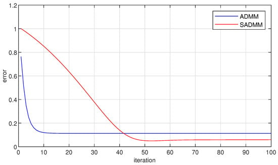
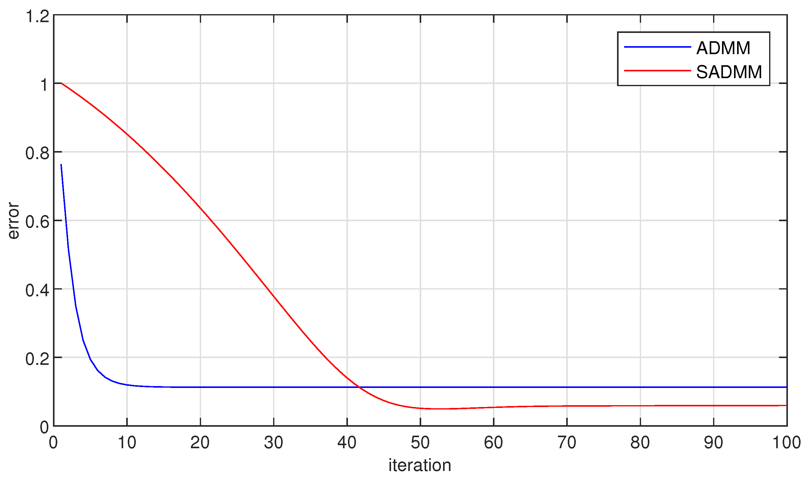
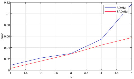
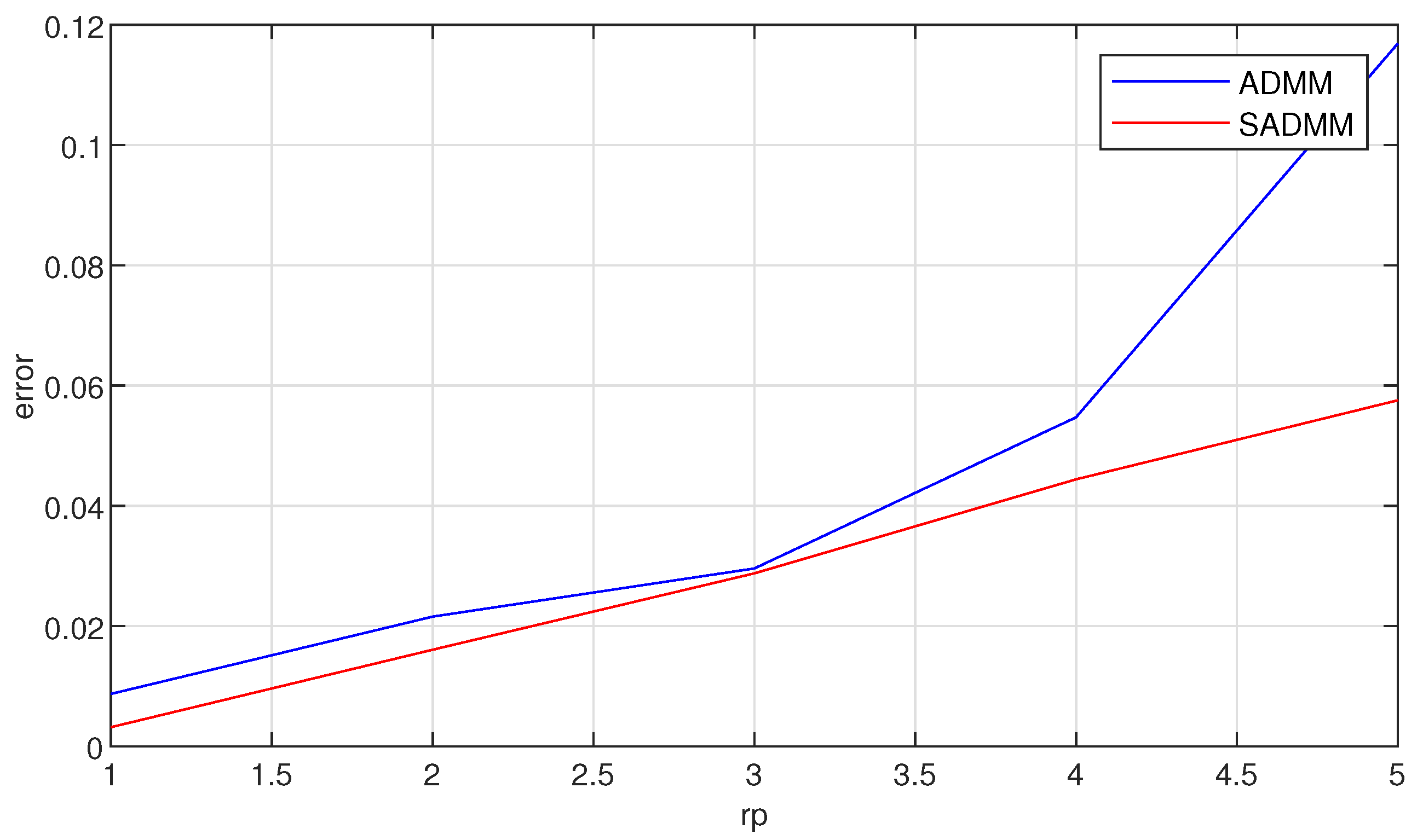
We use our improved S-ADMM algorithm to compare it with the traditional ADMM algorithm. Figure 1 shows the error comparison between the S-ADMM algorithm and the ADMM algorithm at different numbers of iterations. As can be seen from the figure, the error of the S-ADMM algorithm is always smaller than that of the ADMM algorithm as the number of iterations increases. Table 1 shows the error comparison of the two algorithms at different iteration errors. It is clearly seen that the error of the S-ADMM algorithm is significantly smaller than that of the conventional ADMM algorithm. To show the robustness of the S-ADMM algorithm, we compare the errors of the S-ADMM algorithm and the ADMM algorithm at different . According to Figure 2 and Table 2, when the rank of the matrix increases, the trend of increasing error of S-ADMM is always smaller than that of the ADMM algorithm.
Figure 1.
The matrix recovery error under different numbers of iterations.
Table 1.
Errors under different numbers of iterations.
Figure 2.
The matrix recovery error under different levels of rank parameter .
Table 2.
Errors under different levels of rank parameter.
5.2. Experiment Results with Real Data
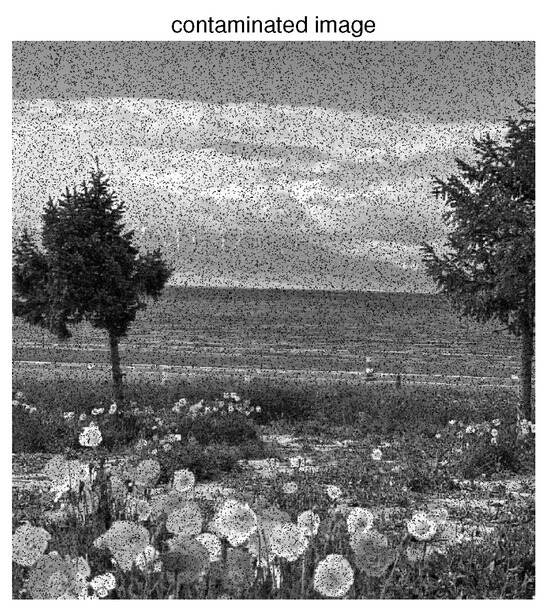
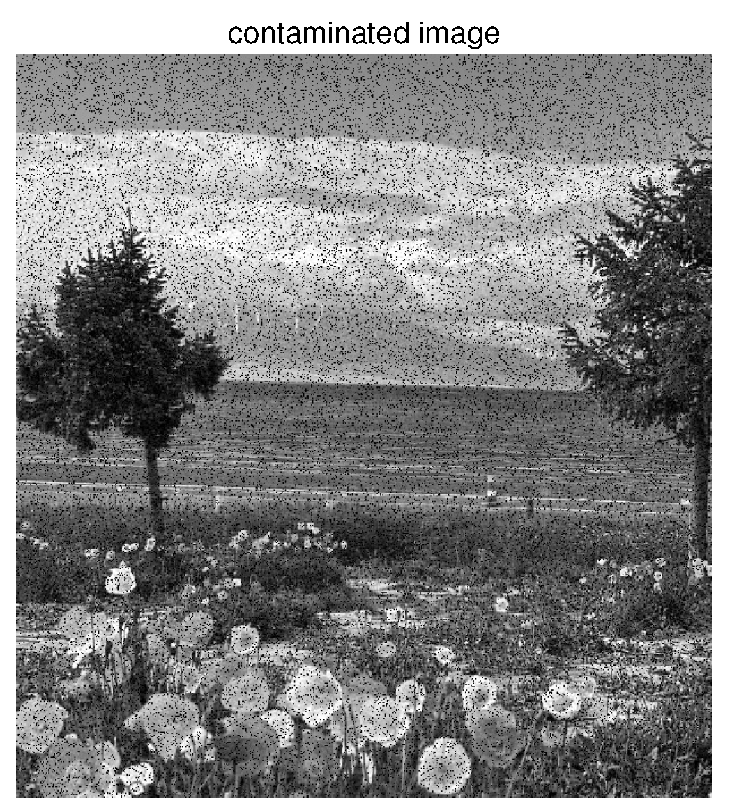
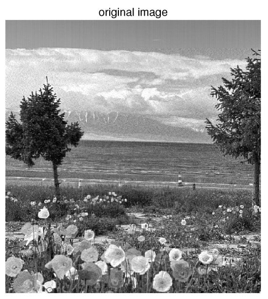
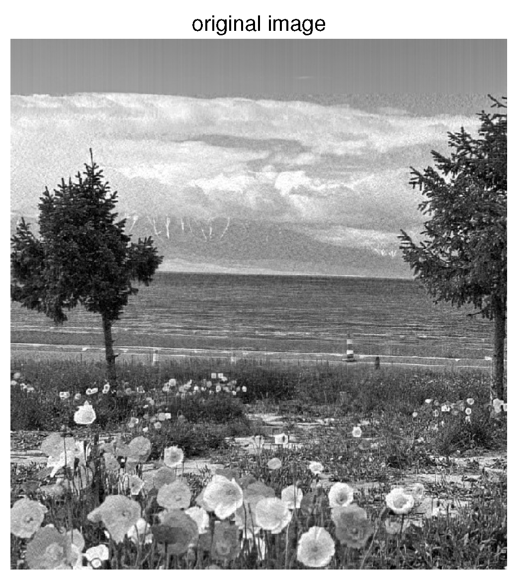
In this section, our algorithmic proposition is substantiated through the empirical validation conducted on two distinct grayscale images sourced from a publicly available dataset. These images exhibit dimensions of and , respectively, thereby providing a diverse testing ground for our methodology. To emulate real-world image corruption scenarios, a deliberate contamination process was introduced. Specifically, 10% of the pixel values were systematically set to 0, while an additional 10% underwent the introduction of random high-level noise. This meticulous contamination scheme was adopted to mimic common noise patterns observed in practical image acquisition and transmission scenarios.
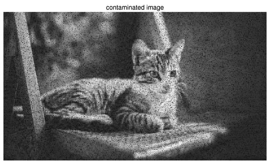
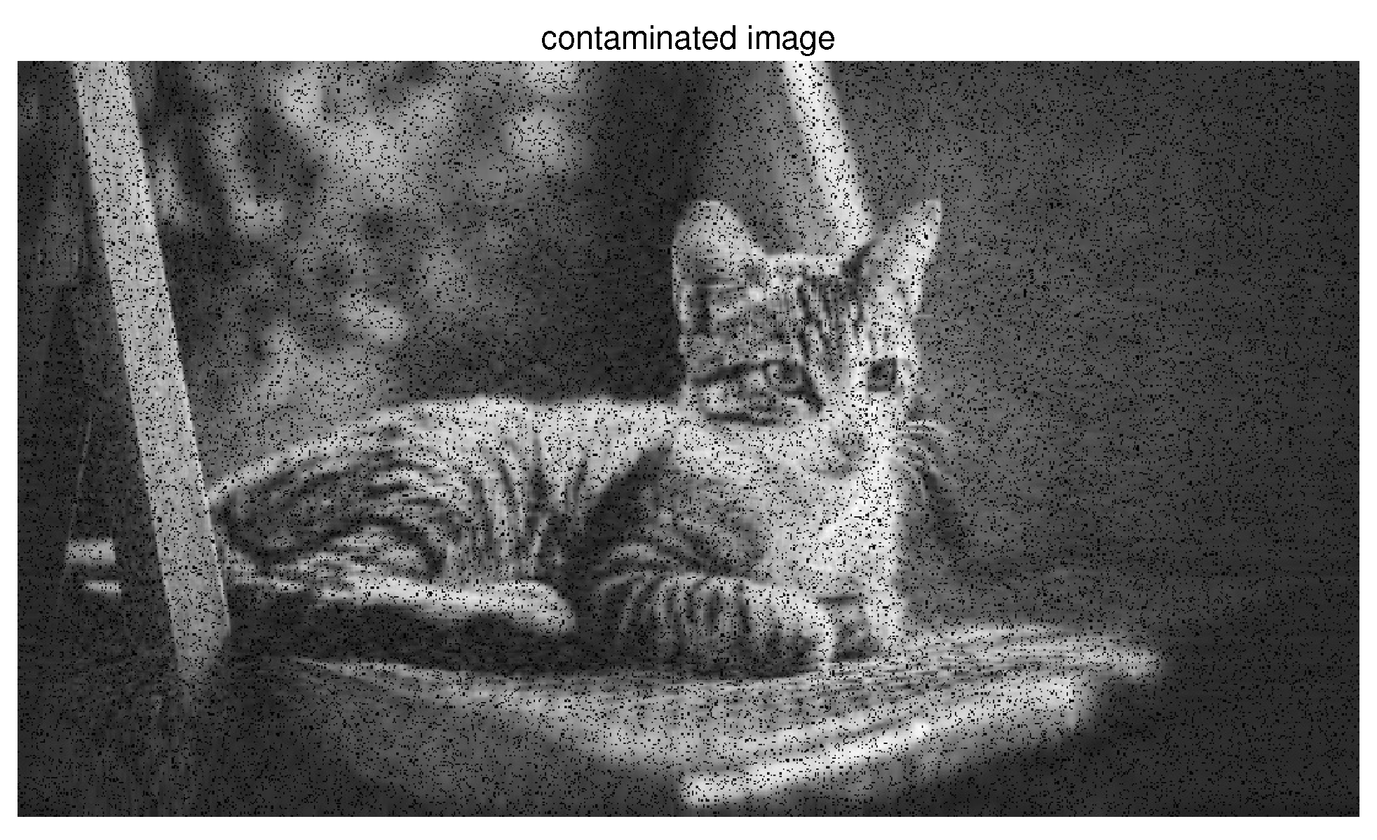
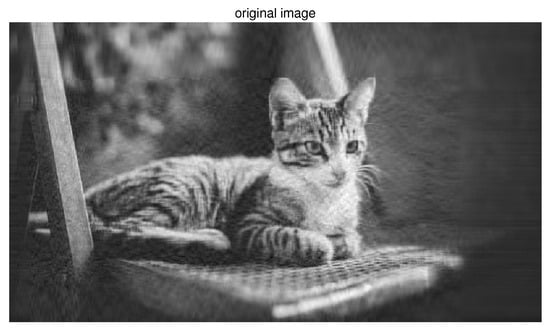
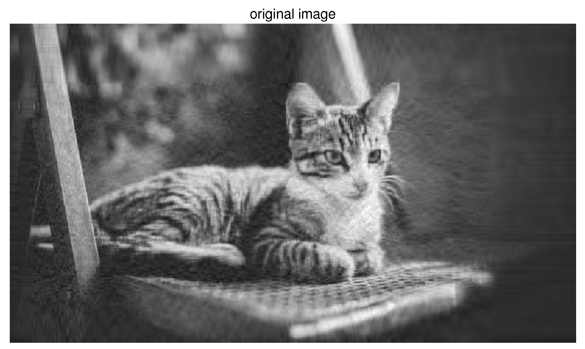
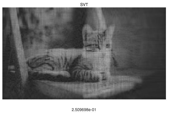
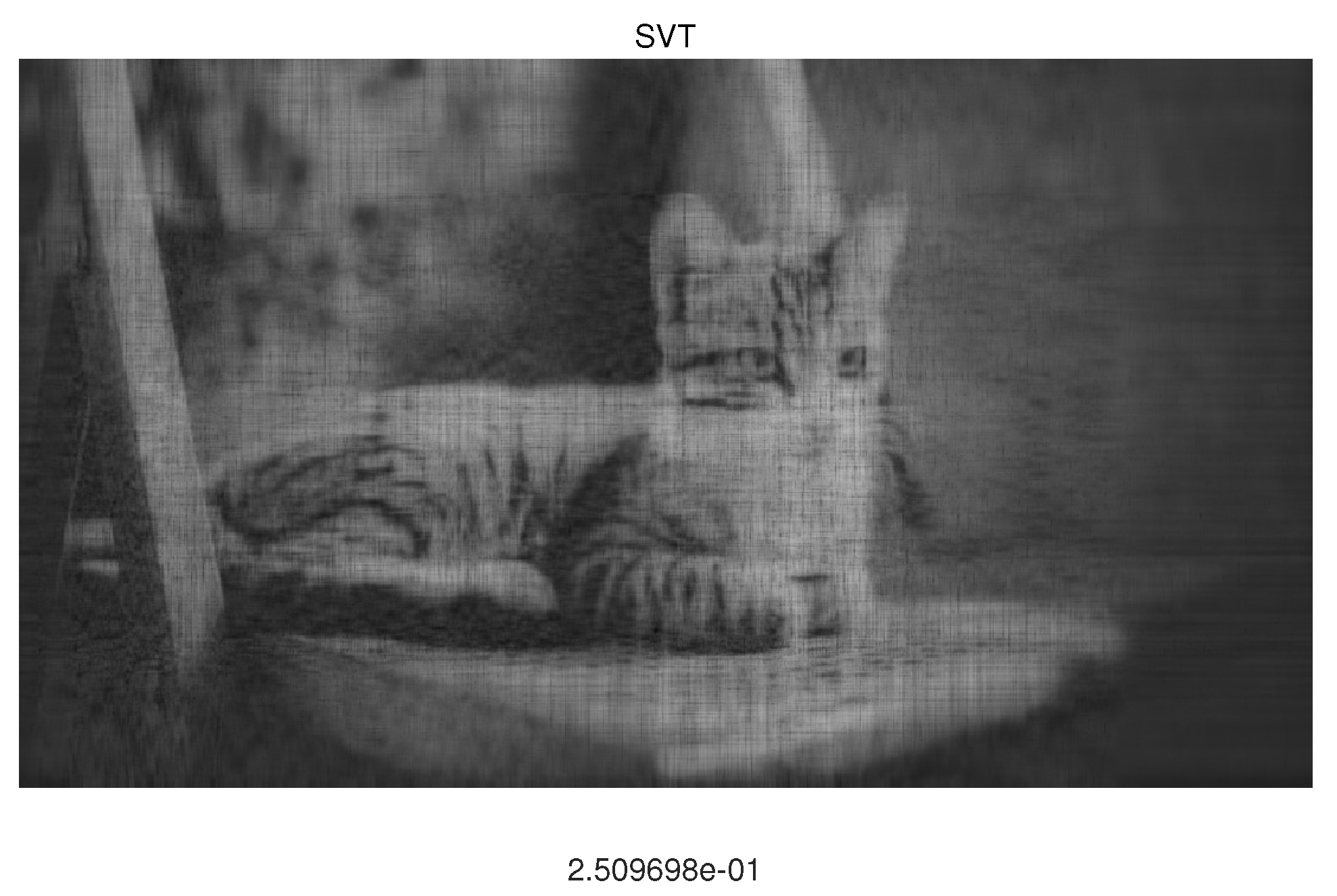
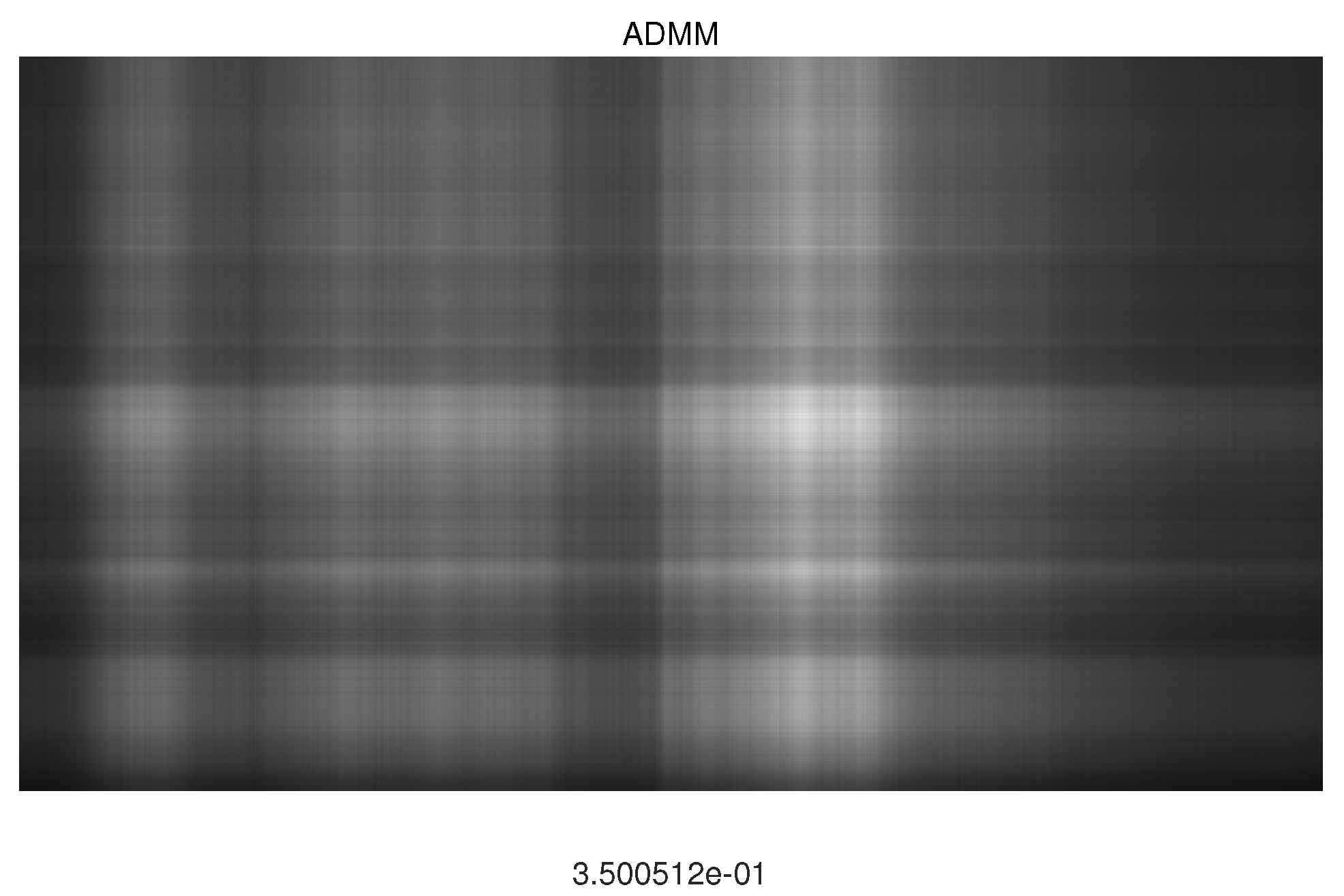
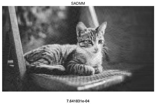
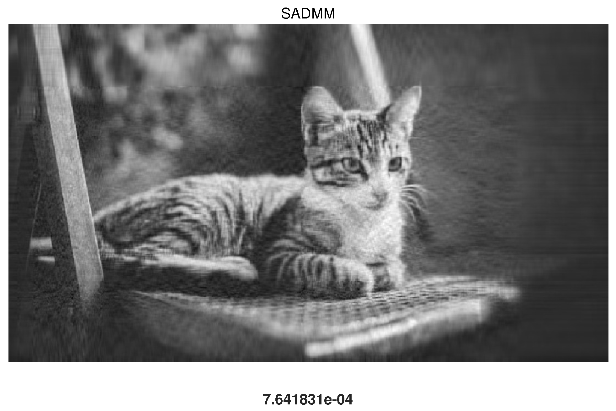
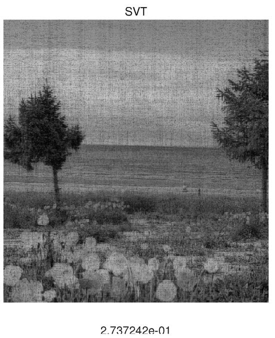
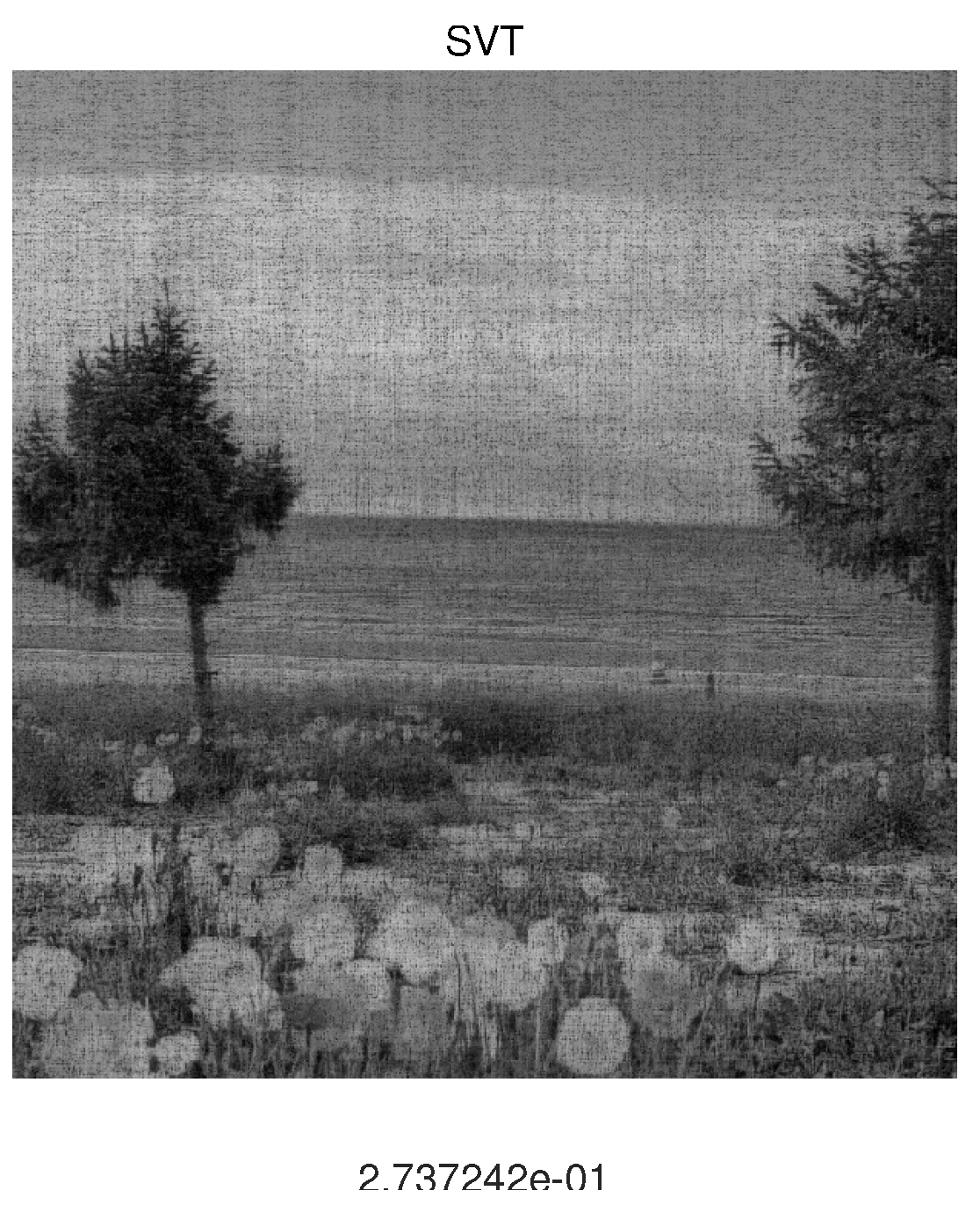
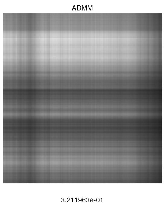
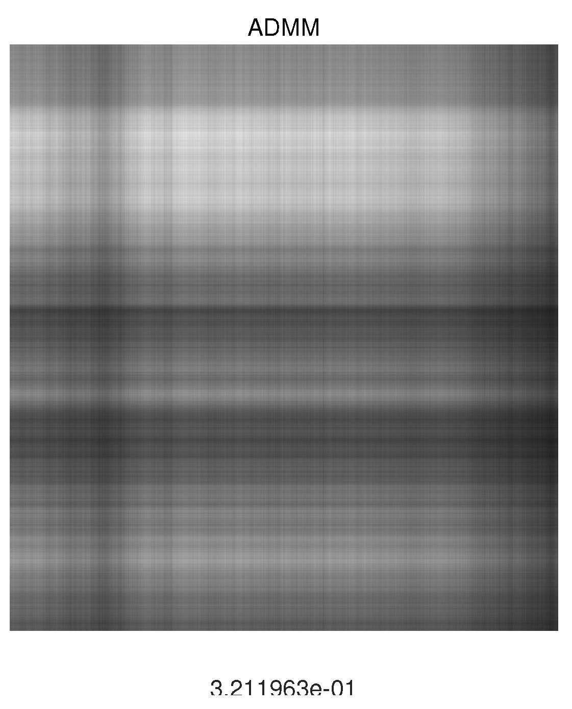
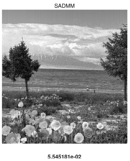
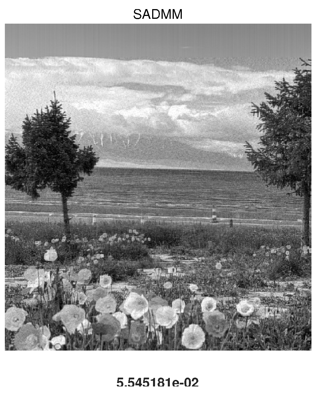
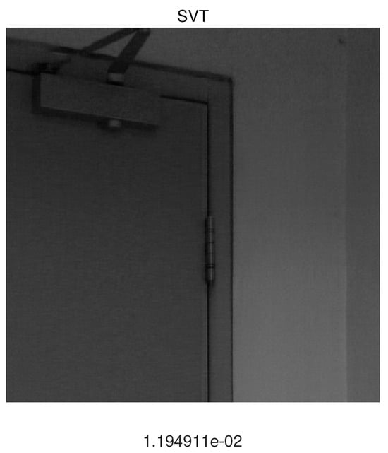
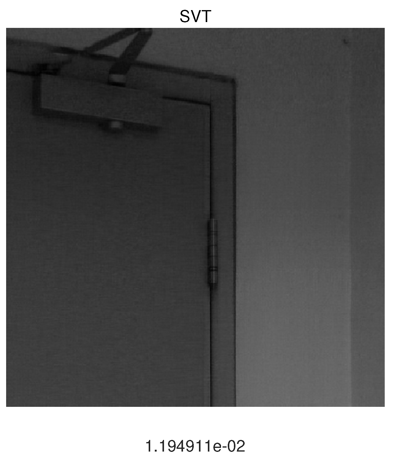
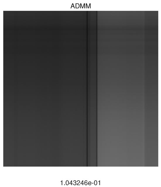
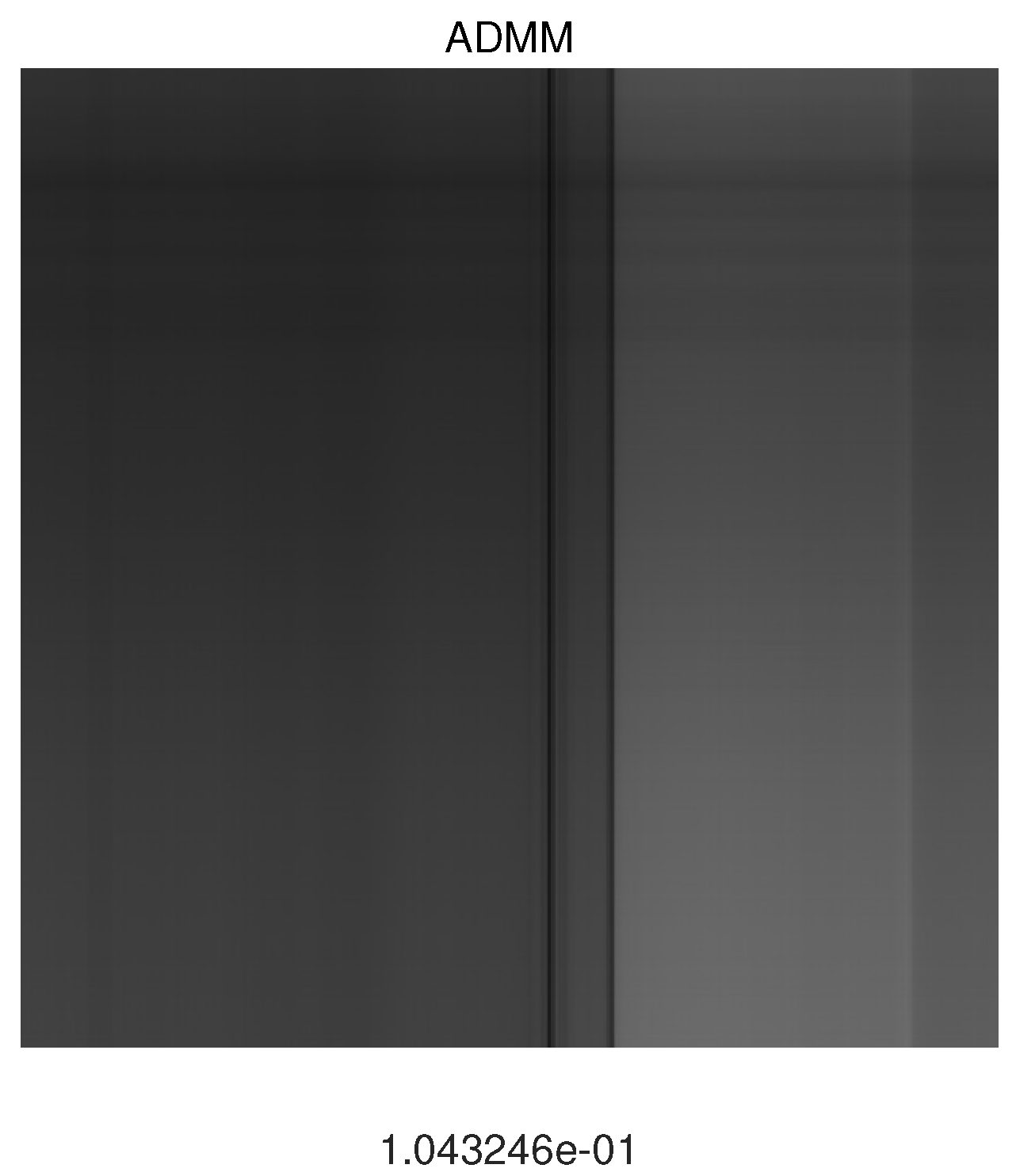
Subsequent to the contamination stage, the denoising process was initiated employing a repertoire of state-of-the-art algorithms, including Singular Value Thresholding (SVT), Alternating Direction Method of Multipliers (ADMM), and the Self-adaptive ADMM (S-ADMM) technique. This multi-faceted approach was undertaken to comprehensively evaluate the efficacy of our algorithm across a spectrum of noise levels and image sizes. Figure 3 represents the first grayscale image after contamination, while Figure 4, Figure 5, Figure 6 and Figure 7 show the denoising effects under different algorithms. Figure 8, Figure 9, Figure 10, Figure 11 and Figure 12 demonstrate the denoising effects under different algorithms for a larger pixel size image. The mean squared error between the denoised image and the ground truth image can be found in Table 3 and Table 4.
Figure 3.
Contaminated grayscale image .
Figure 4.
Original image .
Figure 5.
Denoising effects using SVT algorithms .
Figure 6.
Denoising effects using ADMM algorithms .
Figure 7.
Denoising effects using S-ADMM algorithms .
Figure 8.
Contaminated grayscale image .
Figure 9.
Original image .
Figure 10.
Denoising effects using SVT algorithms .
Figure 11.
Denoising effects using ADMM algorithms .
Figure 12.
Denoising effects using S-ADMM algorithms .
Table 3.
MSE and SSIM from different algorithms .
Table 4.
MSE and SSIM from different algorithms .
5.3. Experiment Results with Real Noisy Images
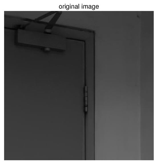
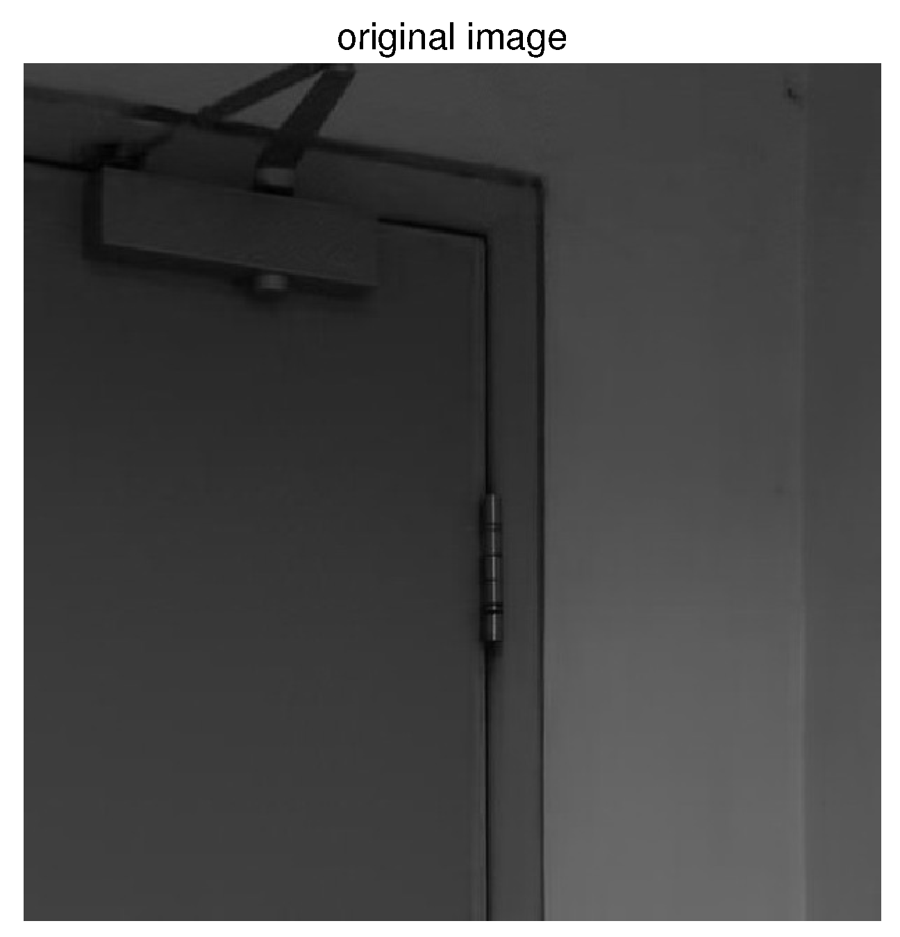
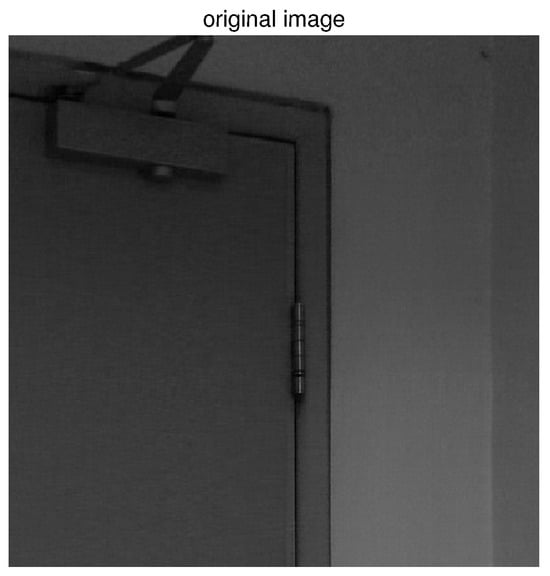
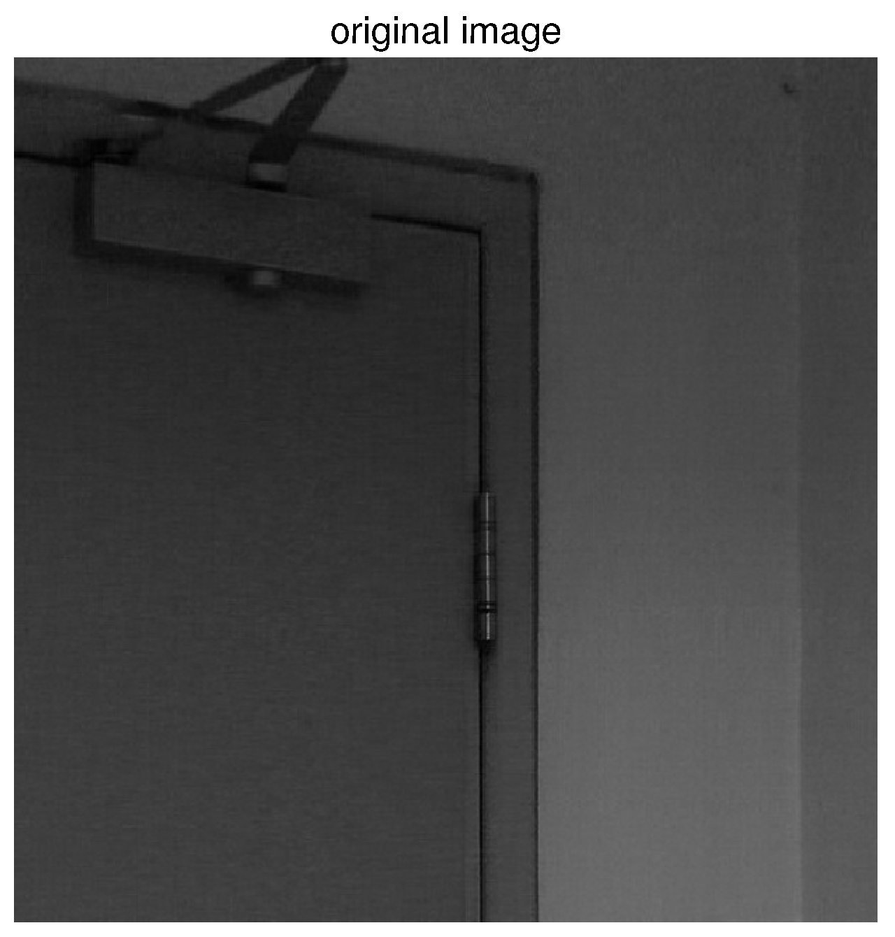
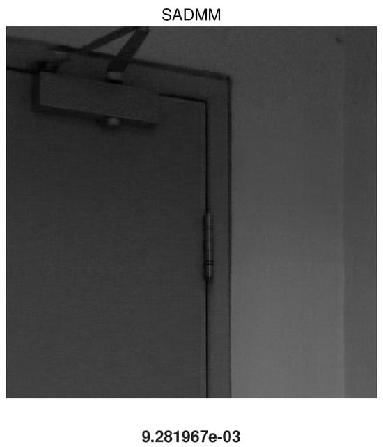
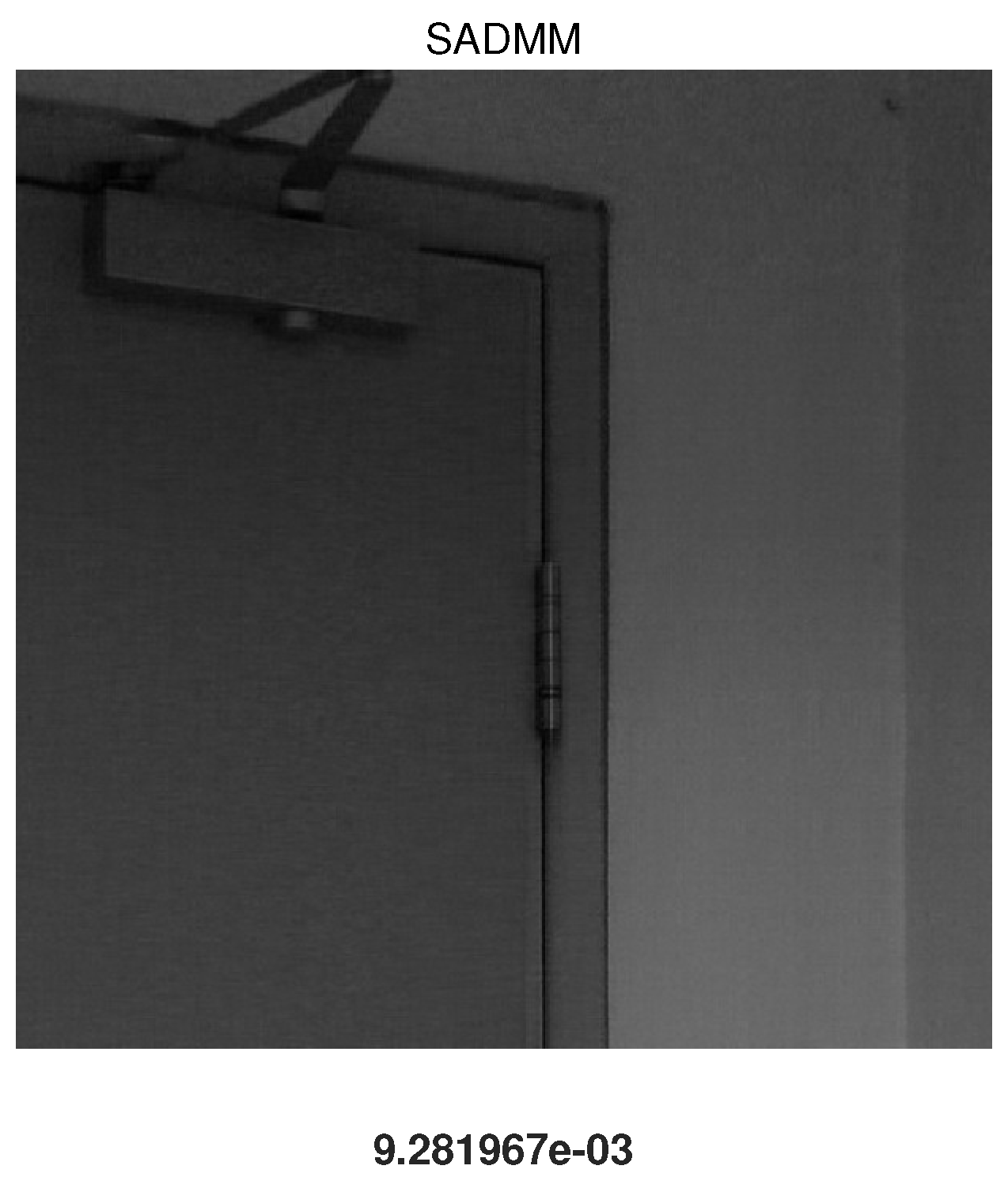
In this section, we employed real-world noisy images to evaluate the performance of our proposed algorithm. The data were sourced from a benchmark image denoising database, PolyUDataset [34]. The data were acquired using a Sony A7II ILCE-7M2 camera, manufactured by Sony Corporation in Tokyo, Japan, with an Aperture of f/4, Shutter Speed of 1/200 s, and ISO Value of 3200. The dataset was generated by capturing multiple shots of the same static scene and computing the average image to create the ground truth image for a more accurate assessment of denoising method performance. We selected one frame from these noisy images, with pixel dimensions of .
Figure 13 and Figure 14, respectively, display the ground truth image and the original noisy image. Singular Value Thresholding (SVT), Alternating Direction Method of Multipliers (ADMM), and the Self-adaptive ADMM (S-ADMM) technique were individually applied to process the noisy image, with results shown in Figure 15, Figure 16 and Figure 17. The final mean square error and structural similarity index of the algorithms are presented in Table 5. These results indicate that our proposed S-ADMM method has the best performance.
Figure 13.
Groundtruth image .
Figure 14.
Noisy image .
Figure 15.
Denoising effects using SVT algorithms .
Figure 16.
Denoising effects using ADMM algorithms .
Figure 17.
Denoising effects using S-ADMM algorithms .
Table 5.
MSE and SSIM from different algorithms .
6. Discussion
The S-ADMM method proposed in this paper, incorporating collaborative sparse regression, has established an effective sparse representation, advancing the exploration of structured sparsity and spatial relationships among pixels. Our adaptive approach has shown remarkable performance in mitigating the impact of penalty parameters on algorithm effectiveness. These findings hold significant implications for the field of image processing, offering insights for enhancing image quality and denoising efficacy. Future research directions could delve into the effectiveness of sparse representation methods, and extend the application of this method to other areas of image processing, thereby driving the development of image processing technologies.
7. Conclusions
In this paper, we proposed a self-adaptive alternating direction method of multipliers for image denoising. By employing collaborative sparse regression, a common sparse representation can be discovered, maintaining structured sparsity within the image and facilitating a more profound exploration of spatial interrelations among pixels. To mitigate the impact of penalty parameters on convergence rates, an adaptive approach based on a balance principle for selecting appropriate penalty parameters is introduced. The experimental results demonstrate that the proposed S-ADMM algorithm yields significantly superior image quality. Other potential enhancements, such as further increasing denoising effectiveness, will be subject to further investigation. Future work could involve integrating deep learning techniques to enhance the performance of the algorithm on complex image data. Additionally, further analysis on multimodal data processing could be conducted to extend the algorithm’s applications to a wider range of scenarios.
Author Contributions
Conceptualization, H.G.; Data curation, M.X.; Methodology, M.X.; Validation, M.X.; Visualization, M.X.; Writing—original draft, M.X.; Writing—review and editing, H.G. All authors have read and agreed to the published version of the manuscript.
Funding
This research received no external funding.
Institutional Review Board Statement
Not applicable.
Informed Consent Statement
Not applicable.
Data Availability Statement
The original contributions presented in the study are included in the article; further inquiries can be directed to the corresponding author.
Conflicts of Interest
The authors declare no conflicts of interest.
Abbreviations
The following abbreviations are used in this manuscript:
| MDPI | Multidisciplinary Digital Publishing Institute |
| DOAJ | Directory of Open-Access Journals |
| TLA | Three-letter acronym |
| LD | Linear dichroism |
References
- Jain, V.; Seung, H. Natural Image Denoising with Convolutional Networks. Adv. Neural Inf. Process. Syst. 2008, 24, 769–776. [Google Scholar]
- Liu, D.; Li, D.; Song, H. Image Quality Assessment Using Regularity of Color Distribution. IEEE Access 2016, 4, 4478–4483. [Google Scholar] [CrossRef] [Scilit]
- Kim, J.; Lee, J.K.; Lee, K.M. Accurate image super-resolution using very deep convolutional networks. In Proceedings of the IEEE Conference on Computer Vision and Pattern Recognition, Las Vegas, NV, USA, 27–30 June 2016; pp. 1646–1654. [Google Scholar]
- Tian, C.; Xu, Y.; Fei, L.; Yan, K. Deep Learning for Image Denoising: A Survey. In Advances in Intelligent Systems and Computing, Proceedings of the ICGEC 2018, Changzhou, China, 14–17 December 2018; Springer: Singapore, 2019; Volume 834. [Google Scholar]
- Puttagunta, M.; Ravi, S. Medical image analysis based on deep learning approach. Multimed. Tools Appl. 2021, 80, 24365–24398. [Google Scholar] [CrossRef] [Scilit]
- Vo, H.H.P.; Nguyen, T.M.; Yoo, M. Weighted Robust Tensor Principal Component Analysis for the Recovery of Complex Corrupted Data in a 5G-Enabled Internet of Things. Appl. Sci. 2024, 14, 4239. [Google Scholar] [CrossRef] [Scilit]
- Zhang, H.; Huang, D.; Wang, K. Denoising of Wrapped Phase in Digital Speckle Shearography Based on Convolutional Neural Network. Appl. Sci. 2024, 14, 4135. [Google Scholar] [CrossRef] [Scilit]
- Yi, J.; Jiang, H.; Wang, X. A Comprehensive Review on Sparse Representation and Compressed Perception in Optical Image Reconstruction. Arch. Comput. Methods Eng. 2024, 31, 3197–3209. [Google Scholar] [CrossRef] [Scilit]
- Yuan, Q.; Zhang, Q.; Li, J.; Shen, H.; Zhang, L. Hyperspectral image denoising employing a spatial–spectral deep residual convolutional neural network. IEEE Trans. Geosci. Remote Sens. 2019, 57, 1205–1218. [Google Scholar] [CrossRef] [Scilit]
- Bodrito, T.; Zouaoui, A.; Chanussot, J.; Mairal, J. A trainable spectral–spatial sparse coding model for hyperspectral image restoration. Proc. Adv. Neural Inf. Process. Syst. 2021, 34, 5430–5442. [Google Scholar]
- Bampis, E.; Escoffier, B.; Schewior, K.; Teiller, A. Online Multistage Subset Maximization Problems. Algorithmica 2021, 83, 2374–2399. [Google Scholar] [CrossRef] [Scilit]
- Eom, M.; Han, S.; Park, P. Statistically unbiased prediction enables accurate denoising of voltage imaging data. Nat. Methods 2023, 20, 1581–1592. [Google Scholar] [CrossRef] [Scilit]
- Buades, A.; Coll, B.; Morel, J.-M. A non-local algorithm for image denoising. In Proceedings of the 2005 IEEE Computer Society Conference on Computer Vision and Pattern Recognition, San Diego, CA, USA, 20–26 June 2005; Volume 2, pp. 60–65. [Google Scholar]
- Zhang, K.; Zuo, W.; Chen, Y.; Meng, D.; Zhang, L. Beyond a Gaussian Denoiser: Residual Learning of Deep CNN for Image Denoising. IEEE Trans. Image Process. 2017, 26, 3142–3155. [Google Scholar] [CrossRef] [Scilit] [PubMed]
- Candes, E.J.; Li, X.; Ma, Y.; Wright, J. Robust Principal Component Analysis? J. ACM 2011, 58, 37. [Google Scholar] [CrossRef] [Scilit]
- Muksimova, S.; Umirzakova, S.; Mardieva, S.; Cho, Y.I. Enhancing Medical Image Denoising with Innovative Teacher–Student Model-Based Approaches for Precision Diagnostics. Sensors 2023, 23, 9502. [Google Scholar] [CrossRef] [Scilit] [PubMed]
- Chen, Y.; Jalali, A.; Sanghavi, S.; Caramanis, C. Low-Rank Matrix Recovery From Errors and Erasures. IEEE Trans. Inf. Theory 2013, 59, 4324–4337. [Google Scholar] [CrossRef] [Scilit]
- Muksimova, S.; Mardieva, S.; Cho, Y.I. Deep Encoder–Decoder Network-Based Wildfire Segmentation Using Drone Images in Real-Time. Remote Sens. 2022, 14, 6302. [Google Scholar] [CrossRef] [Scilit]
- Li, X.; Zhu, Z.; Man-Cho So, A.; Vidal, R. Nonconvex Robust Low-Rank Matrix Recovery. SIAM J. Optim. 2020, 30, 660–686. [Google Scholar] [CrossRef] [Scilit]
- Huan, X.; Caramanis, C.; Sanghavi, S. Robust PCA via outlier pursuit. IEEE Trans. Inf. Theory 2012, 58, 3047–3064. [Google Scholar]
- Recht, B. A simpler approach to matrix completion. J. Mach. Learn. Res. 2011, 12, 3413–3430. [Google Scholar]
- Koko, J. Parallel Uzawa method for large-scale minimization of partially separable functions. J. Optim. Theory Appl. 2013, 158, 172–187. [Google Scholar] [CrossRef] [Scilit]
- Liu, Y.; Jiao, L.C.; Shang, F.; Yin, F.; Liu, F. An efficient matrix bi-factorization alternative optimization method for low-rank matrix recovery and completion. Neural Netw. 2013, 48, 8–18. [Google Scholar] [CrossRef] [Scilit]
- Hu, Y.; Liu, X.; Jacob, M. A Generalized Structured Low-Rank Matrix Completion Algorithm for MR Image Recovery. IEEE Trans. Med. Imaging 2019, 38, 1841–1851. [Google Scholar] [CrossRef] [Scilit] [PubMed]
- Iordache, M.D.; Bioucas-Dias, J.M.; Plaza, A. Collaborative Sparse Regression for Hyperspectral Unmixing. IEEE Trans. Geosci. Remote Sens. 2014, 52, 341–354. [Google Scholar] [CrossRef] [Scilit]
- Zhang, S.G. Projection and self-adaptive projection methods for the Signorini problem with the BEM. Appl. Math. Comput. 2017, 74, 1262–1273. [Google Scholar] [CrossRef] [Scilit]
- Zhang, S.; Li, X. A self-adaptive projection method for contact problems with the BEM. Appl. Math. Model. 2018, 55, 145–159. [Google Scholar] [CrossRef] [Scilit]
- Huang, Z.; Li, S.; Hu, F. Hyperspectral image denoising with multiscale low-rank matrix recovery. In Proceedings of the 2017 IEEE International Geoscience and Remote Sensing Symposium (IGARSS), Fort Worth, TX, USA, 23–28 July 2017; pp. 5442–5445. [Google Scholar]
- Mason, E.; Yazici, B. Robustness of LRMR based Passive Radar Imaging to Phase Errors. In Proceedings of the EUSAR 2016: 11th European Conference on Synthetic Aperture Radar, Hamburg, Germany, 6–9 June 2016; pp. 1–4. [Google Scholar]
- Zhou, P.; Lu, C.; Feng, J.; Lin, Z.; Yan, S. Tensor Low-Rank Representation for Data Recovery and Clustering. IEEE Trans. Pattern Anal. Mach. Intell. 2021, 43, 1718–1732. [Google Scholar] [CrossRef] [Scilit]
- Shen, Q.; Liang, Y.; Yi, S.; Zhao, J. Fast Universal Low Rank Representation. IEEE Trans. Circuits Syst. Video Technol. 2022, 32, 1262–1272. [Google Scholar] [CrossRef] [Scilit]
- Chen, T.; Xiang, Q.; Zhao, D.; Sun, L. An Unsupervised Image Denoising Method Using a Nonconvex Low-Rank Model with TV Regularization. Appl. Sci. 2023, 13, 7184. [Google Scholar] [CrossRef] [Scilit]
- Wu, B.; Yu, J.; Ren, H.; Lou, Y.; Liu, N. Seismic Traffic Noise Attenuation Using lp -Norm Robust PCA. IEEE Geosci. Remote Sens. Lett. 2020, 17, 1998–2001. [Google Scholar] [CrossRef] [Scilit]
- Xu, J.; Li, H.; Liang, Z.; Zhang, D.; Zhang, L. Real-world Noisy Image Denoising: A New Benchmark. arXiv 2018, arXiv:1804.02603. [Google Scholar] [CrossRef] [Scilit]

Disclaimer/Publisher’s Note: The statements, opinions and data contained in all publications are solely those of the individual author(s) and contributor(s) and not of MDPI and/or the editor(s). MDPI and/or the editor(s) disclaim responsibility for any injury to people or property resulting from any ideas, methods, instructions or products referred to in the content. |
© 2024 by the authors. Licensee MDPI, Basel, Switzerland. This article is an open access article distributed under the terms and conditions of the Creative Commons Attribution (CC BY) license (https://creativecommons.org/licenses/by/4.0/).