Wind Turbine Performance Evaluation Method Based on Dual Optimization of Power Curves and Health Regions

Abstract

The wind power curve serves as a critical metric for assessing wind turbine performance. Developing a model based on this curve and evaluating turbine efficiency within a defined health region, derived from the statically optimized power curve, holds significant value for wind farm operations. This paper proposes an optimized wind power curve segmentation modeling method based on an improved PCF algorithm to address the inconsistency between the function curve and the wind power curve, as well as the issues of prolonged curve modeling training time and susceptibility to local optima. A health region optimization method based on data increment inflection points is developed, which enables the delineation of the health performance evaluation region for wind turbines. Through the aforementioned optimization, the performance evaluation method for wind turbines is significantly improved. The effectiveness of the performance evaluation method is validated through experimental case studies, combining the wind power curve with the rotational speed stability, power characteristic consistency coefficient, and power generation efficiency indicators. The proposed modeling technique achieves a precision level of 0.998, confirming its applicability and effectiveness in practical engineering scenarios.

1. Introduction

Amid the rapid expansion of wind energy as a sustainable power source, there has been a concerted effort by governmental bodies to foster technological innovation and advancements. This drive aims at enhancing the development and deployment of wind generation technologies, boosting the efficiency and dependability of wind energy systems. Concurrently, there is an emphasis on the meticulous planning and management of wind farm infrastructure, refining the spatial distribution of wind energy resources to augment the operational efficiency and cumulative benefits of these installations. The imperative for real-time health and performance assessments of wind turbines stems from their potential to preemptively identify and rectify equipment malfunctions, thereby ensuring the uninterrupted operation of wind farms. Turbine performance, a pivotal factor in the wind energy conversion process, significantly influences the power generation capacity, reliability, and cost-effectiveness of wind turbines. Turbines that exhibit high performance are adept at capturing and converting wind energy into electricity, maximizing energy yield. In this context, the wind power curve emerges as a crucial metric for turbine performance appraisal, instrumental in evaluating energy production, efficiency metrics, power forecasting, and health monitoring. The body of research dedicated to the application of wind power curve modeling in turbine performance assessment is progressively expanding.

1.1. Modeling of Wind Power Curves

Regarding the modeling of wind power curves, prevalent methodologies encompass approaches grounded in the binning method, polynomial regression, and B-spline curve fitting.

• Binning Method for Wind Power Curve Modeling.

• Yang Mao et al. introduced a modeling approach using the binning method to articulate the relationship between wind velocity and generated power, examining the variability in modeling errors across different wind speed segments [1]. Similarly, Peng Lin et al. undertook a comparative analysis among the maximum value, maximum probability, and binning methods for modeling wind power curves. They highlighted the binning method’s closer alignment with real-world turbine operations based on empirical data [2]. In addressing challenges posed by deterministic turbine output models’ inability to precisely characterize statistical features of wind energy production, Chen et al. refined power data analysis using an enhanced binning technique and data fitting processes to mitigate data interference [3]. Likewise, to accurately quantify production losses in individual turbines, Zhan et al. devised the GD-BIN method (Gaussian distribution and bins), creating a wind power curve model that accurately reflects each turbine’s efficiency [4]. The GPR class method necessitates the random sampling of historical data for each prediction, resulting in high computational demands and reduced prediction stability [5].

• Polynomial Fitting for Wind Power Curve Modeling.

• Engaging with power curve data selection and fitting processes, researchers employed advanced polynomial and logistic function fitting algorithms for wind speed–power curve modeling after data refinement. Comparative evaluations of model accuracy and efficiency revealed that polynomial fitting, with its straightforward principle, rapid fitting capability, and commendable accuracy, is well-suited for practical power curve modeling tasks [6,7]. Xu et al. proposed an optimized local polynomial regression technique to develop an adaptive robust model for time-variant scatter power curves, aimed at enhancing predictive accuracy [8]. Through linear least squares, Wang et al. assessed various polynomial regression models, identifying those offering superior approximations for diverse wind speed distributions [9].

• B-Spline Fitting for Wind Power Curve Modeling.

• Recent scholarly efforts have also embraced B-spline fitting for curve modeling. Research documented in [10] applied the Iteratively Reweighted Least Absolute Shrinkage and Selection Operator (Lasso) for complex autoregressive modeling with periodic B-splines, accommodating diurnal and annual variations. Investigating four curve fitting approaches, ref. [11] advanced discussions on polynomial fitting by introducing methodologies such as local weighted polynomial fitting, cubic spline fitting, and cubic B-spline curve fitting to elevate fitting precision and adaptability. An innovative wind power curve modeling technique, employing enhanced smooth splines for wind speed–power data fitting, was outlined in [12]. This approach utilized cubic splines for data approximation and applied a roughness penalty for coefficient regularization, with cross-validation determining the optimal smoothing parameters. Addressing the modeling and optimization challenges in small-sample scenarios with complex mixed-type parameter interactions, ref. [13] proposed a novel strategy integrating Gaussian process regression with B-spline curves. This method constructed a functional parameter model through a weighted combination of B-spline-based functions and control points, followed by a genetic algorithm for model optimization.

The investigations cited previously have significantly advanced the modeling of wind power curves. Nonetheless, when translating these advancements into practical settings, two primary challenges emerge. Firstly, the discrepancies between mathematical function curves and empirical wind power curves present a notable challenge. Within the realm of practical engineering, achieving a precise correlation between these curves often proves elusive, undermining the accuracy of the resulting models. Secondly, the extended duration required for model training and the propensity for models to converge on local optima rather than global solutions compound the complexity of this endeavor. This not only extends the time required to develop usable models but also risks entrenching suboptimal solutions.

These impediments contribute to elevated modeling errors and protracted model fitting periods. Addressing these challenges necessitates the development of an innovative approach to wind power curve modeling. Such an approach should cater to the practical demands for model smoothness, accuracy, efficiency, and adaptability, thereby laying a more robust foundation for the utility of power curves in future applications.

1.2. Evaluation of Wind Turbine Performance Utilizing Wind Power Curves

The realm of wind turbine performance assessment currently employs methodologies grounded in wind power curve analysis and artificial intelligence-driven evaluations [14,15,16,17,18,19,20,21]. The former approach, notable for its ease of modeling and quantification capabilities, is exemplified by a method proposed in [22]. This method enhances the precision in defining the evaluation parameters by calculating the limits of automatic power curves, thus facilitating a robust assessment of turbine health through a comprehensive analysis of deviations between actual and ideal static power curves, alongside efficiency metrics.

To summarize, the operational health of turbines is contingent upon a multitude of factors, including environmental conditions, hardware integrity, and control mechanisms. Reference [23] posits that wind energy is a renewable resource, with wind power generation harnessing this energy for electricity production. Wind speed serves as an indicator of the magnitude of wind energy, while wind speed–power data directly reflect the efficiency of wind energy capture by wind turbines. Among these data, the most significant correlation is observed between wind speed and power. The establishment of a wind power curve model that accurately mirrors real-time turbine operation enables the substantive assessment of turbine health. In light of this, this study introduces a refined polynomial curve fitting (PCF) algorithm tailored for wind power curve modeling. This novel approach, coupled with a method to ascertain turbine health regions via data increment inflection points, aims to elevate the precision in turbine performance evaluation. This paper’s novel contributions are outlined as follows:

• The incorporation of a regularization term within the least squares framework propels an enhanced segmented modeling optimization technique for the wind power curve via the refined PCF algorithm. This innovation addresses the challenges of curve–function disparities and the extensive duration required for model training, potentially affected by local optima, thereby paving new avenues in health performance curve modeling for turbines.
• Leveraging the proposed optimization algorithm for wind power curve modeling, this study devises an optimized approach to defining health regions grounded in data increment inflection points. This delineation fosters a solid foundation for the subsequent evaluation of turbine health performance.

This study pioneers the integration of wind power curves with parameters such as rotor speed stability, consistency in power characteristics, and efficiency metrics, facilitating a comprehensive assessment of turbine health. This methodology underscores the efficacy of the proposed turbine performance evaluation framework.

2. Materials and Methods

2.1. An Enhanced Approach to Wind Power Curve Optimization via the Improved PCF Algorithm

Initially, a comprehensive data cleansing operation is undertaken on the extensive dataset of raw wind speed and power readings. This cleansing employs a combination of Lagrange interpolation, the quartile method, and the MeanShift clustering algorithm, yielding a refined set of preliminary wind speed–power data. Subsequently, this dataset, segmented according to the binning method, undergoes a process of standardization and power adjustment to derive the refined wind speed–power data. The culmination of this process involves the integration of the PCF algorithm, grounded in the principles of least squares and augmented with a ridge regression regularization component, with a B-spline fitting algorithm for segmented modeling. This sophisticated approach facilitates the generation of the theoretical static optimal power curve.

2.1.1. The Binning Method

The binning method orchestrates the segmentation of wind speed into $\mathrm{M}$ equal intervals, each designated as a bin. Assigning a width of 0.5 m/s to each bin, the methodology involves computing the mean wind speed ${\mathrm{v}}_{\mathrm{i}\mathrm{m}\mathrm{e}\mathrm{a}\mathrm{n}}$ and power ${\mathrm{P}}_{\mathrm{i}\mathrm{m}\mathrm{e}\mathrm{a}\mathrm{n}}$ for the data points within each bin, ultimately yielding $\mathrm{M}$ arrays of data pairs $({\mathrm{v}}_{\mathrm{i}\mathrm{m}\mathrm{e}\mathrm{a}\mathrm{n}},{\mathrm{P}}_{\mathrm{i}\mathrm{m}\mathrm{e}\mathrm{a}\mathrm{n}})$. The calculations are guided by the following expressions:

$${\mathrm{v}}_{\mathrm{i}\mathrm{m}\mathrm{e}\mathrm{a}\mathrm{n}}=\frac{1}{{\mathrm{n}}_{\mathrm{i}}}\sum _{\mathrm{j}=1}^{{\mathrm{n}}_{\mathrm{i}}}{\mathrm{v}}_{\mathrm{i}\mathrm{j}}$$

(1)

$${\mathrm{P}}_{\mathrm{i}\mathrm{m}\mathrm{e}\mathrm{a}\mathrm{n}}=\frac{1}{{\mathrm{n}}_{\mathrm{i}}}\sum _{\mathrm{j}=1}^{{\mathrm{n}}_{\mathrm{i}}}{\mathrm{P}}_{\mathrm{i}\mathrm{j}}$$

(2)

In the above equation, the subscript $\mathrm{i}$ denotes the placement of data within the nth bin; ${\mathrm{n}}_{\mathrm{i}}$ signifies the count of data points; ${\mathrm{v}}_{\mathrm{i}\mathrm{m}\mathrm{e}\mathrm{a}\mathrm{n}}$ and ${\mathrm{P}}_{\mathrm{i}\mathrm{m}\mathrm{e}\mathrm{a}\mathrm{n}}$ represent the mean wind speed and power, respectively; and ${\mathrm{v}}_{\mathrm{i}\mathrm{j}}$ and ${\mathrm{P}}_{\mathrm{i}\mathrm{j}}$ are the wind speed and power readings of the $\mathrm{j}$-th data point within the bin, respectively.

2.1.2. Adjustment of Power Outputs

The generation capacity of wind turbines exhibits a direct correlation with the ambient air density, necessitating the conversion of manufacturer-provided power curves to those applicable under standardized atmospheric conditions. Under these standard conditions, characterized by a defined air density ${\mathsf{\rho }}_0=1.225 \mathrm{k}\mathrm{g}/{\mathrm{m}}^3$ and atmospheric pressure ${\mathrm{P}}_0=101.33 \mathrm{k}\mathrm{P}\mathrm{a}$, the conversion is governed by the following relationship:

$$\frac{{\mathrm{P}}_0}{\mathrm{P}}=\frac{{\mathsf{\rho }}_0}{\mathsf{\rho }}$$

(3)

This leads to the derivation of wind speeds and power outputs under standard conditions, as expressed by

$${\mathrm{v}}_{\mathrm{N}}={\mathrm{v}}_{10\mathrm{m}\mathrm{i}\mathrm{n}}·{(\frac{{\mathsf{\rho }}_{10\mathrm{m}\mathrm{i}\mathrm{n}}}{\mathsf{\rho }})}^{\frac{1}{3}}$$

(4)

$${\mathrm{P}}_{\mathrm{N}}={\mathrm{P}}_{10\mathrm{m}\mathrm{i}\mathrm{n}}·\frac{\mathsf{\rho }}{{\mathsf{\rho }}_{10\mathrm{m}\mathrm{i}\mathrm{n}}}$$

(5)

In the above equation, ${\mathrm{v}}_{\mathrm{N}}$ symbolizes the air density-normalized wind speed, with ${\mathrm{v}}_{10\mathrm{m}\mathrm{i}\mathrm{n}}$ denoting the mean wind speed over a 10 min interval. Similarly, ${\mathrm{P}}_{\mathrm{N}}$ represents the air density-adjusted power output, with ${\mathrm{P}}_{10\mathrm{m}\mathrm{i}\mathrm{n}}$ indicating the mean power output over the same duration. $\mathsf{\rho }$ stands for the standard air density, while ${\mathsf{\rho }}_{10\mathrm{m}\mathrm{i}\mathrm{n}}$ refers to the mean air density measured over a 10 min span.

It is important to note that the power adjustments described herein pertain to the net power delivered to the grid by the generator, distinct from the raw values depicted in the initial power curve. The latter does not account for the energy consumption inherent to the turbine’s operation. To bridge this gap and align closer with the theoretical power curve, one must deduct the turbine’s internal energy expenditure from the measured output values. Estimating this consumption can be achieved by contrasting the power outputs recorded at wind speeds surpassing the rated threshold against the nominal power specified in the original curve. This comparison facilitates a preliminary assessment of the turbine’s operational energy demand.

2.1.3. Refinement of the PCF Algorithm

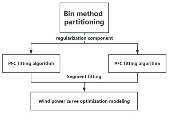
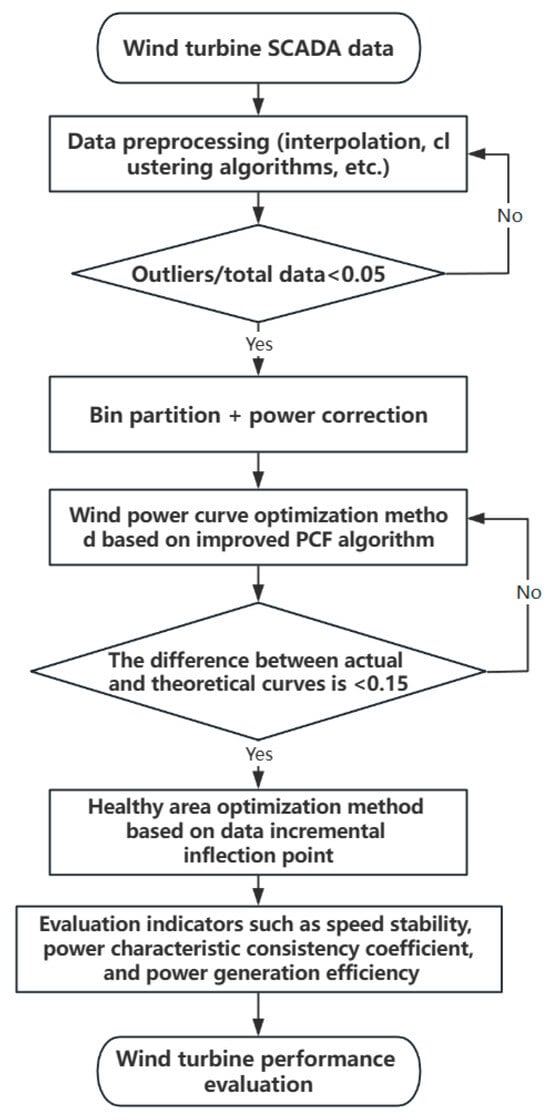
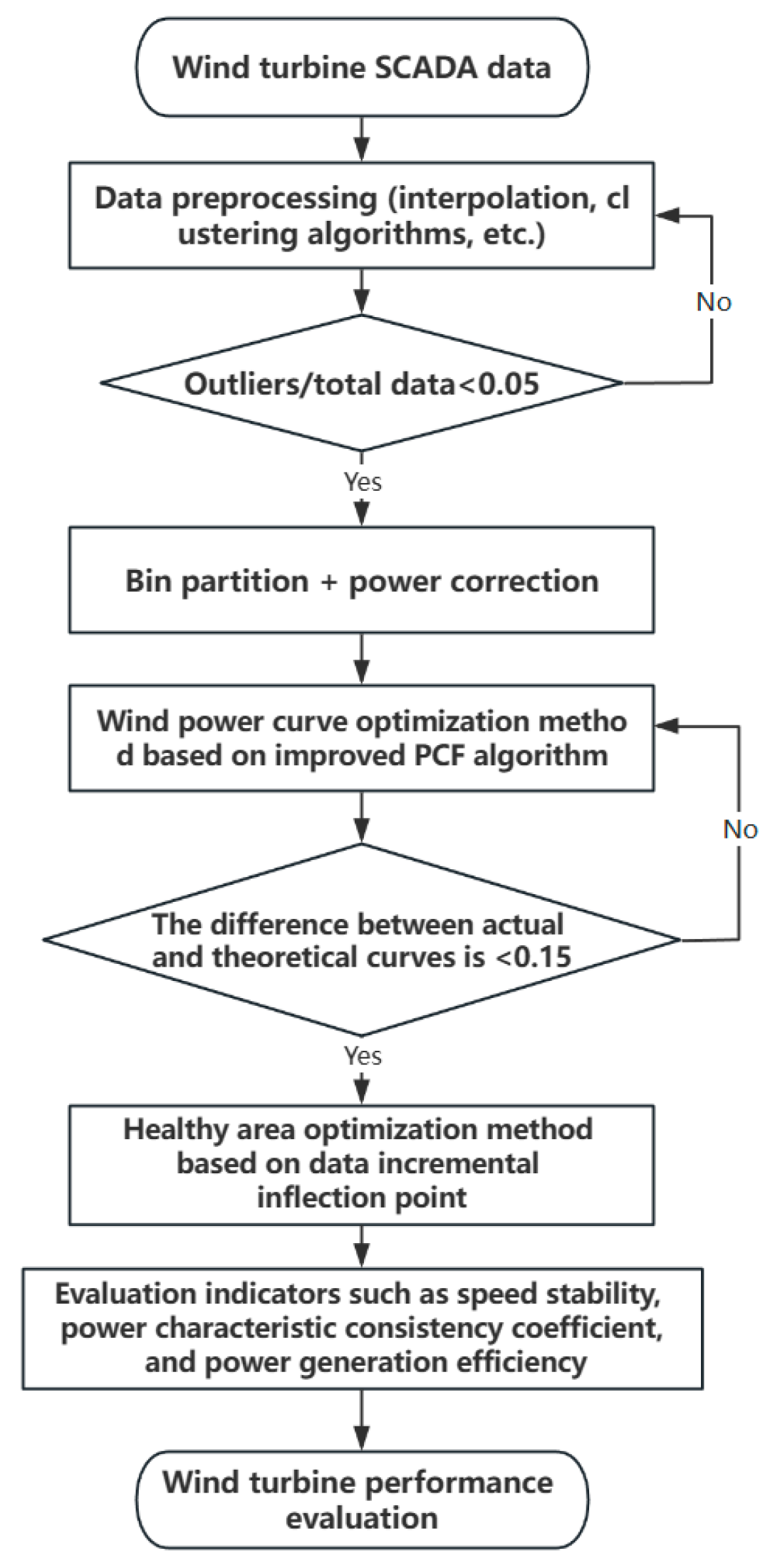
As delineated in Figure 1, the refined PCF algorithm commences with the standardized corrections of power data categorized by the Bin method, culminating in the acquisition of finalized wind speed–power datasets. A pivotal enhancement involves the integration of a ridge regression regularization component into the PCF framework, traditionally grounded in the least squares methodology. This addition, coupled with the employment of B-spline fitting for segmented modeling, facilitates the derivation of a theoretically ideal static power curve. The algorithm operates on the following foundational principles:

Figure 1. Improved PCF algorithm flow.

• PCF Algorithm Foundation:

Consider a training dataset represented by:

$$D=[\left(x_1,y_1\right),\left(x_2,y_2\right),\left(x_3,y_3\right)\dots ({\mathit{x}}_{\mathit{N}},{\mathit{y}}_{\mathit{N}}\left)\right]$$

(6)

At its core, the polynomial fitting approach functions as a linear model articulated by the following equation:

$$y(x,\omega )=\sum _{j=0}^M{\mathit{\omega }}_{\mathit{j}}{\mathit{x}}_{\mathit{i}}^{\mathit{j}}$$

(7)

In this formula, $\mathrm{M}$ is the highest degree of the polynomial, ${\mathrm{x}}_{\mathrm{i}}^{\mathrm{j}}$ represents the j-power of ${\mathrm{x}}_{\mathrm{i}}$, and ${\mathsf{\omega }}_{\mathrm{j}}$ is the coefficient of ${\mathrm{x}}_{\mathrm{i}}^{\mathrm{j}}$.

The crux of the fitting process lies in devising an error metric to evaluate the accuracy of the polynomial approximation. This involves formulating a model parameterized by $\mathsf{\theta }$, which, upon processing $\mathrm{x}$ inputs, yields predicted outcomes. The model’s refinement phase employs training data ${\mathrm{x}}_{\mathrm{i}}$ to generate predictions, subsequently measuring the deviation $\mathrm{L}$ from the actual values ${\mathrm{y}}_{\mathrm{i}}$. Model optimization is achieved by iteratively adjusting parameter $\mathsf{\theta }$ to minimize this discrepancy until an optimal congruence between prediction and reality is attained. The error metric is thus a function crafted to quantify the disparity between these predicted and actual values, encapsulated by $\mathsf{\theta }$.

The dataset encompasses $\mathrm{N}$ samples, with each ${\mathrm{x}}_{\mathrm{n}}$ being associated with an output ${\mathrm{t}}_{\mathrm{n}}$. Adopting square loss as the evaluation metric and introducing coefficients $\frac{1}{2}$ to streamline computations, the loss function, upon integration of the model and training data, is articulated as

$$E(\omega )=\frac{1}{2}\sum _{n=1}^M{\{y\left({\mathit{x}}_{\mathit{n}},\omega \right)-{\mathit{t}}_{\mathit{n}}\}}^2$$

(8)

Taking the partial derivative ${\mathsf{\omega }}_{\mathrm{j}}$ and setting it to zero,

$$\begin{gathered} Let\frac{\partial L\left(\omega \right)}{\partial {\omega }_k}=0\stackrel{\hspace{0.17em}}{\Rightarrow } \\ \frac{1}{2}\sum _{i=1}^{N}2\left(\sum _{j=0}^M{\omega }_j{x}_i^j-y_i\right)x_i^{j+k}=0\stackrel{\hspace{0.17em}}{\Rightarrow } \\ \sum _{i=1}^N\sum _{j=0}^M{\omega }_j{x}_i^j=\sum _{i=1}^N{x}_i^k{y}_i(k=0,1,2\dots ,M) \end{gathered}$$

(9)

The quest for polynomial coefficients ${\mathsf{\omega }}_0^{\mathrm{*}},{\mathsf{\omega }}_1^{\mathrm{*}},{\mathsf{\omega }}_2^{\mathrm{*}},\dots ,{\mathsf{\omega }}_{\mathrm{M}}^{\mathrm{*}}$ necessitates solving the ensuing system of linear equations:

$$\left[\begin{array}{cccc}N& {\displaystyle \sum X_i^{\hspace{0.17em}}}& \dots & {\displaystyle \sum X_i^M}\\ {\displaystyle \sum X_i^{\hspace{0.17em}}}& {\displaystyle \sum X_i^2}& \dots & {\displaystyle \sum X_i^{M+1}}\\ {\displaystyle \sum X_i^2}& {\displaystyle \sum X_i^3}& \dots & {\displaystyle \sum X_i^{M+2}}\\ {\displaystyle \sum X_i^M}& {\displaystyle \sum X_i^{M+1}}& \dots & {\displaystyle \sum X_i^{2M}}\end{array}\right]\left(\begin{array}{c}{\omega }_0\\ {\omega }_1\\ {\omega }_2\\ ⋮\\ {\omega }_m\end{array}\right)=\left[\begin{array}{c}{\displaystyle \sum y_i}\\ {\displaystyle \sum x_i^{\hspace{0.17em}}{y}_i}\\ {\displaystyle \sum x_i^2{y}_i}\\ ⋮\\ {\displaystyle \sum x_i^M{y}_i}\end{array}\right]$$

(10)

The calculation is as follows:

$$\sum _{i=1}^N{\mathit{x}}_{\mathit{i}}^{\mathit{j}}(j=0,1,2,\dots ,2M)$$

(11)

$$\sum _{i=1}^N{\mathit{x}}_{\mathit{i}}^{\mathit{j}}{\mathit{y}}_{\mathit{i}}(j=0,1,2,\dots ,M)$$

(12)

Substituting these determinations into the system facilitates the resolution of the polynomial coefficients, marking the completion of the model’s optimization.

2.

B-Spline Fitting Algorithm

The utilization of the PCF algorithm for wind power curve modeling has shown commendable efficacy in the segments preceding the turbine’s rated power output. However, its fitting effect tends to wane in the sections post-rated power, where data stability is more pronounced. In this context, B-spline fitting emerges as a robust alternative, demonstrating superior adaptability and fitting accuracy in these latter segments. The strategic integration of both methodologies, through a segmented fitting approach, enhances the model’s adaptability across the entire power spectrum, thereby elevating the precision of the overall wind power curve modeling.

B-splines are a special class of spline function, where, as the name suggests, B-splines serve as the basis for general spline functions. For n + 2 nodes ${\mathsf{\xi }}_1<\dots <{\mathsf{\xi }}_{\mathrm{n}+2}$, the function expression in Formula (13) can prove that the nth-degree spline function, which is 0 outside the interval, forms a one-dimensional linear space, the basis of which is

$$B_{\left[{\mathsf{\xi }}_1,{\mathsf{\xi }}_{n+2}\right],n+1}\left(x\right)=\frac{x-{\mathsf{\xi }}_1}{{\mathsf{\xi }}_{n+1}-{\mathsf{\xi }}_1}{B}_{\left[{\mathsf{\xi }}_1,{\mathsf{\xi }}_{n+2}\right],n}\left(x\right)+\frac{{\mathsf{\xi }}_{n+2}-\mathrm{x}}{{\mathsf{\xi }}_{n+1}-{\mathsf{\xi }}_2}{B}_{\left[{\mathsf{\xi }}_2,{\mathsf{\xi }}_{n+2}\right],n}\left(x\right)$$

(13)

In the above equation, $\mathrm{n}+1$ signifies an n + 1 degree spline function in ${\mathrm{B}}_{\left[{\mathsf{\xi }}_1,{\mathsf{\xi }}_{\mathrm{n}+2}\right],\mathrm{n}+1}$, correlating with an nth-degree spline in terms of its operational order (the degree and order of spline functions always differ by 1).

The construction of a finite-dimensional linear space, predicated on a predefined node sequence $[{\mathsf{\xi }}_1,{\mathsf{\xi }}_{\mathrm{m}}]$ coupled with nth-degree spline functions, is instrumental in the fitting process. The selection of appropriate basis functions is pivotal, significantly influencing computational efficiency. The intrinsic merit of B-spline functions lies in their provision of a convenient and computationally tractable set of bases for spline function fitting. These bases, characterized by their nullity beyond the nodal points, facilitate the segmentation of the interval $[{\mathsf{\xi }}_1,{\mathsf{\xi }}_{\mathrm{m}}]$ into manageable subintervals and find the basis of the spline function in each small interval. By splicing these basis functions, the basis of the spline function on the interval $[{\mathsf{\xi }}_1,{\mathsf{\xi }}_{\mathrm{m}}]$ can be obtained, thus facilitating subsequent curve modeling operations.

3.

Regularized least squares

In the endeavor of curve fitting, vigilance against overfitting and local oscillatory behavior is paramount. These challenges predominantly arise from limited data interspersed with noise, where an overfitting model might endeavor to accommodate every data point, noise included, thereby escalating the count of coefficients within the fitting function. Addressing overfitting typically involves two strategies: reducing the dimensionality of the sample features and employing parameter regularization, which entails the incorporation of a penalty term. Regularization serves to impose constraints on the coefficients under determination, thereby streamlining them and enhancing the model’s generalization capacity.

Regularization is conventionally implemented by appending a regularization term to the composite average loss function. In the context of regularized least squares, denoted as, this entails the integration of a regularization component during the least squares computation of PCF coefficients, thereby yielding a regularized estimate for the least squares of the function $\mathrm{E}\left(\mathsf{\omega }\right)$. This process involves the incorporation of the sum of squares of all polynomial fitting coefficients into the penalty model, coupled with the delineation of a penalty intensity factor $\mathsf{\omega }$. This factor is pivotal in circumventing the emergence of aberrant coefficients. A frequently employed penalty function, aimed at forestalling overfitting, is represented as

$$Q=\sum _{i=1}^n{(y\left({\mathit{x}}_{\mathit{i}},W\right)-{\mathit{t}}_{\mathit{i}})}^2+{\frac{\lambda }{2}||\omega ||}^2$$

(14)

This function introduces a balancing act between fitting the data and maintaining model simplicity, thereby mitigating the risk of overfitting while preserving the model’s predictive integrity.

In the formula, ${\frac{\mathsf{\lambda }}{2}||\mathsf{\omega }||}^2$ represents the regularization term, ${||\mathsf{\omega }||}^2={\mathsf{\omega }}^{\mathrm{T}}\mathsf{\omega }={\mathsf{\omega }}_0^2+{\mathsf{\omega }}_1^2+\dots +{\mathsf{\omega }}_{\mathrm{M}}^2$ associated with ridge regression, and $\mathsf{\lambda }$ is the smoothing parameter that dictates the level of penalty applied to the roughness of the data, with larger $\mathsf{\lambda }$ values leading to greater losses.

The regularization term consists of the sum of the decay constant $\mathsf{\lambda }$ multiplied by the ridge regression. In cases of limited sample data, the modeling curve attempts to fit all data points, including noise, resulting in a large number of coefficients that tend to be oversized. The regularization term in Equation (15) aims to minimize the influence of noise points by reducing the sum of the squares of $\mathsf{\omega }$ to smaller absolute values, thus penalizing larger coefficients. Introducing the regularization term helps to prevent overfitting and enhances the model’s generalization capability.

In wind power curve modeling using the improved PCF algorithm, selecting the optimal $\mathsf{\lambda }$ parameter is crucial. The goal of parameter selection is to balance between improving data fit and minimizing model complexity, favoring the simplest model that adequately fits the wind speed–power data. An excessively large $\mathsf{\lambda }$ can overly suppress the model, making the choice of an appropriate $\mathsf{\lambda }$ critical for the final fitting result of the model. This choice should be made based on the complexity of the model, with cross-validation (CV) used to determine the optimal value.

$$C_V(\lambda )=min\left\{\frac{1}{N}\sum _{i=1}^N{(y\left({\mathit{x}}_{\mathit{i}},W\right)-{\mathit{t}}_{\mathit{i}})}^2\right\}$$

(15)

In this equation, N represents the number of data points. The $\mathsf{\lambda }$ value that minimizes the generalization error ${\mathrm{C}}_{\mathrm{V}}\left(\mathsf{\lambda }\right)$ is considered the optimal parameter.

In the wind power curve modeling process using the improved PCF algorithm, data preprocessing is a key step that significantly contributes to the accuracy of the modeling. Although it is impossible to eliminate all outliers during the preprocessing phase, there will still be a few noise points that affect the smoothness and precision of the wind power curve. By employing the aforementioned methods, the impact of these noise points can be maximally reduced, thereby enhancing the accuracy and reliability of the modeling.

2.1.4. Evaluation Metrics for Wind Power Curve Modeling

Given the band-like scatter distribution of the original wind speed–power data, there exists a certain level of discrepancy between the fitted power curve and the actual data. Minimizing this error leads to a more accurate representation of the overall power generation capability of the unit. This paper focuses on two main aspects for evaluating the power curve modeling: modeling efficiency and accuracy. The evaluation metrics include the mean absolute error (MAE), the root mean squared error (RMSE), and the coefficient of determination R² (R-Square), which gauge the precision of the model. Additionally, the modeling time is also considered as an evaluation metric to assess the efficiency of the modeling process.

$$NMAE=\frac{1}{m}\sum _{i=1}^m\left|{\mathit{y}}_{\mathit{i}}-\widehat{{\mathit{y}}_{\mathit{i}}}\right|$$

(16)

$$NRMSE=\sqrt{\frac{1}{m}\sum _{i=1}^m{({\mathit{y}}_{\mathit{i}}-\widehat{{\mathit{y}}_{\mathit{i}}})}^2}$$

(17)

$$R^2=1-\frac{{\sum }_{i=1}^m{(\widehat{{\mathit{y}}_{\mathit{i}}}-{\mathit{y}}_{\mathit{i}})}^2}{{\sum }_{i=1}^m{(\widehat{{\mathit{y}}_{\mathit{i}}}-\overline{{\mathit{y}}_{\mathit{i}}})}^2}$$

(18)

In these formulas, ${\mathrm{y}}_{\mathrm{i}}$ represents the actual power data, $\overline{{\mathrm{y}}_{\mathrm{i}}}$ is the mean value of the actual power data, $\widehat{{\mathrm{y}}_{\mathrm{i}}}$ is the fitted power data, $\mathrm{i}$ is the $\mathrm{i}$-th data in the test dataset, and $\mathrm{m}$ is the number of test sample data.

The MAE assesses how closely the wind power curve fitting results align with the test power data, with smaller values indicating better fitting, as calculated in Equation (16). The RMSE measures the deviation between the actual power data and the fitted power data of the wind power curve, as described in Equation (17). An R² value closer to 1 signifies a stronger representational capability of the fitted curve to the actual power data, as determined by Equation (18).

2.2. Optimization Method for Wind Turbine Health Region Based on Data Increment Inflection Points

Defining the evaluation region is a crucial step in wind turbine performance assessment. However, the original wind power data in this study do not follow a normal distribution, making the use of confidence intervals for region delineation inaccurate and potentially impacting the subsequent wind turbine performance evaluation process.

To enhance the reliability of the wind turbine performance evaluation region, this paper considers the concept of moving the wind turbine power curve (hereafter referred to as the “moving power curve”) and delineates the performance evaluation region for the turbine by analyzing changes in the quantity of wind speed–power data after movement. To facilitate this discussion, the term “data increment inflection point” is introduced, referring to the “wind speed–power” coordinate point where a sudden change in the data increment between the static optimal power curve and the moving power curve reaches a certain threshold. In practical engineering applications, this threshold can be set to 1.16.

The following approach is employed to delineate the health region of the wind turbine: using the absolute value of the slope of the data increment curve to represent the degree of change in data quantity. When a sudden change in data quantity occurs for the first time between the moving power curve and the static optimal power curve, the “data increment inflection point” as defined above appears. At this point, it can be considered that the moving power curve has reached the boundary of the wind turbine performance evaluation region, thereby delineating the performance evaluation region for the wind turbine.

Delineation of Wind Turbine Performance Evaluation Region

To define the health performance region of the wind turbine and accurately assess its health performance, an optimization method based on data increment inflection points is proposed for the wind turbine health region. The process is as follows.

• After cleaning the original wind speed–power data using interpolation and clustering algorithms, the data are grouped into wind speed intervals of 0.5 m/s using the binning method, after sorting the wind speed–power data in ascending order. The average wind speed and power values within each interval, ${\mathrm{v}}_{\mathrm{i}\mathrm{m}\mathrm{e}\mathrm{a}\mathrm{n}}$ and ${\mathrm{P}}_{\mathrm{i}\mathrm{m}\mathrm{e}\mathrm{a}\mathrm{n}}$, are calculated, resulting in $\mathrm{M}$ data pairs $({\mathrm{v}}_{\mathrm{i}\mathrm{m}\mathrm{e}\mathrm{a}\mathrm{n}},{\mathrm{P}}_{\mathrm{i}\mathrm{m}\mathrm{e}\mathrm{a}\mathrm{n}})$.
• Power correction is applied to these $\mathrm{M}$ data pairs $({\mathrm{v}}_{\mathrm{i}\mathrm{m}\mathrm{e}\mathrm{a}\mathrm{n}},{\mathrm{P}}_{\mathrm{i}\mathrm{m}\mathrm{e}\mathrm{a}\mathrm{n}})$.
• The improved PCF algorithm is used to fit these corrected $\mathrm{M}$ data pairs $({\mathrm{v}}_{\mathrm{i}\mathrm{m}\mathrm{e}\mathrm{a}\mathrm{n}},{\mathrm{P}}_{\mathrm{i}\mathrm{m}\mathrm{e}\mathrm{a}\mathrm{n}})$ into a static optimal power curve $\mathrm{T}\mathrm{c}$.
• The power curve $\mathrm{T}\mathrm{c}$ obtained in the previous step is then moved horizontally (step size $∆\mathrm{s}=0.25 \mathrm{m}/\mathrm{s}$) until the data volume percentage ${\mathrm{N}}_{\mathrm{d}}$ between the $\mathrm{n}$-times horizontally moved power curve and the static optimal wind speed–power curve shows its first inflection point on the slope curve. At this point, the movement stops, and the horizontal optimal upper (or lower) limit power curve is determined.

  $$N_d=\frac{{Lc}_n-{Lc}_{Tc}}{D}\times 100\mathrm{\%}$$

  (19)

In Equation (19), $\mathrm{D}$ represents the total data volume of wind power after data cleaning, while ${\mathrm{L}\mathrm{c}}_{\mathrm{n}}-{\mathrm{L}\mathrm{c}}_{\mathrm{T}\mathrm{c}}$ denotes the data volume between the n-th horizontally moved wind power curve and the static optimal wind power curve. Through multiple experimental validations, the best data effect is achieved when ${{\mathrm{N}}_{\mathrm{d}}}^{\mathrm{\prime }}\approx 34.21\mathrm{\%}$ is at a specific value.

• The obtained horizontal optimal power curve is then moved vertically (step size $∆\mathrm{p}=5 \mathrm{K}\mathrm{W}$) until the data volume percentage ${{\mathrm{N}}_{\mathrm{d}}}^{\mathrm{\prime }}$ between the n-th vertically moved power curve and the static optimal power curve reflects the effect demonstrated in the slope curve mentioned in step (4). At this point, the movement stops, and the vertical optimal upper (or lower) limit power curve is established.

  $${N_d}^{\prime }=\frac{{{Lc}_n}^{\prime }-{Lc}_{Tc}}{D}\times 100\mathrm{\%}$$

  (20)

In Equation (20), ${{\mathrm{L}\mathrm{c}}_{\mathrm{n}}}^{\prime }-{\mathrm{L}\mathrm{c}}_{\mathrm{T}\mathrm{c}}$ is the data volume between the n-th vertically moved wind power curve and the static optimal wind power curve. Multiple experimental validations have shown that the best data effect occurs at a specific ${{\mathrm{N}}_{\mathrm{d}}}^{\prime }\approx 34.21\mathrm{\%}$ value.

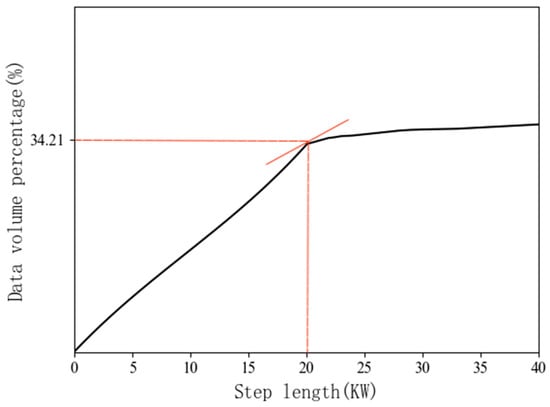
Figure 2 illustrates the data volume change between the power curve, which has already been moved horizontally in step (4), and the static optimal power curve as it undergoes vertical movement. It is evident that when the step size accumulates a movement of approximately 20 kW, and the data volume ${\mathrm{N}}_{\mathrm{d}}$ reaches 34.21%, the absolute value of the slope begins to decrease, and the curve flattens, indicating that the path of movement has reached the optimal vertical limit.

Figure 2. Changes in data volume caused by shifting the power curve.

Figure 3 illustrates the wind turbine performance evaluation process. Initially, the wind power data are segmented using the binning method. Following a power adjustment, an enhanced PCF (power curve fitting) algorithm is employed for curve fitting, leading to the derivation of an optimal static power curve. Subsequently, the assessment region for turbine performance is defined through an optimization approach that leverages inflection points in data increments, establishing the ideal upper and lower boundary power curves for the operational health zone. Ultimately, the actual wind power curve’s behavior within this operational health assessment region is examined, in conjunction with metrics like rotor speed stability, consistency in power characteristics, and generation efficacy, to gauge the turbine’s operational health.

Figure 3. Wind turbine performance evaluation process.

• Rotational Speed Stability

The stability of a wind turbine’s rotational speed is quantifiable by its standard deviation—a statistical indicator used to measure the dispersion of data. In rotor speed data analysis, a smaller standard deviation indicates smaller changes in speed, more stable speed data, suggesting more stable wind turbine operation. In contrast, a higher standard deviation denotes significant speed variability, reflecting potential instability in turbine performance.

Evaluating the standard deviation of rotational speed data over time can thus provide insights into the turbine’s operational stability, with lower values indicating greater stability. This stability is crucial for consistent power output and efficiency in turbine operation. Higher stability helps the wind turbine to maintain a stable output power and has a positive impact on the speed control and operational efficiency of the wind turbine.

2.

Power Performance Coefficient (CP)

The power performance coefficient (CP) measures the alignment between a wind turbine’s actual power output and its theoretical predictions. It is determined by comparing power outputs at various wind speeds, adjusted for air density, to theoretical values. The selection of sampling points between the turbine’s cut-in wind speed and expected theoretical speeds, at intervals of 1 m/s, facilitates this comparison. Assessing the CP across these points allows for a comprehensive evaluation of the turbine’s power efficiency in relation to theoretical models.

$$Cp=1-\frac{SSR}{SST}$$

(21)

In Equation (21), SSR denotes the sum of squares of residuals, representing the discrepancy between actual and theoretical power outputs. SST stands for the total sum of squares, quantifying the variance of actual power outputs from their mean value. A determination coefficient approaching 1 signifies a model’s heightened ability to accurately represent actual power outputs, indicating superior model fitting. The power performance coefficient emerges as a pivotal metric in assessing wind turbine performance.

3.

Efficiency of Power Generation

$$PE=\frac{1}{60}\sum _{i=1}^n\frac{P_r}{P_t}{T}_i(KW·h)$$

(22)

Equation (22) articulates that ${\mathrm{P}}_{\mathrm{r}}$, the real-time power output recorded at 10 min intervals, and ${\mathrm{P}}_{\mathrm{t}}$ theoretical, the anticipated power output, alongside ${\mathrm{T}}_{\mathrm{i}}$ average, the mean duration of power production, serve as foundational elements. Power generation efficiency, typically ranging between 0 and 1, represents the ratio at which wind turbines convert wind energy into electrical power. Enhanced efficiency underscores a turbine’s ability to optimize wind energy for electricity production, thus elevating energy conversion efficiency.

3. Discussion

3.1. Empirical Case Study and Analysis

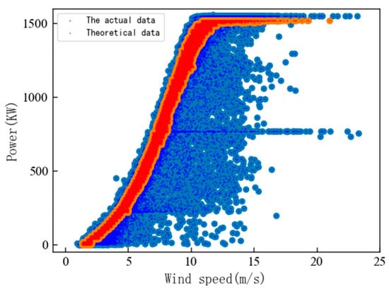
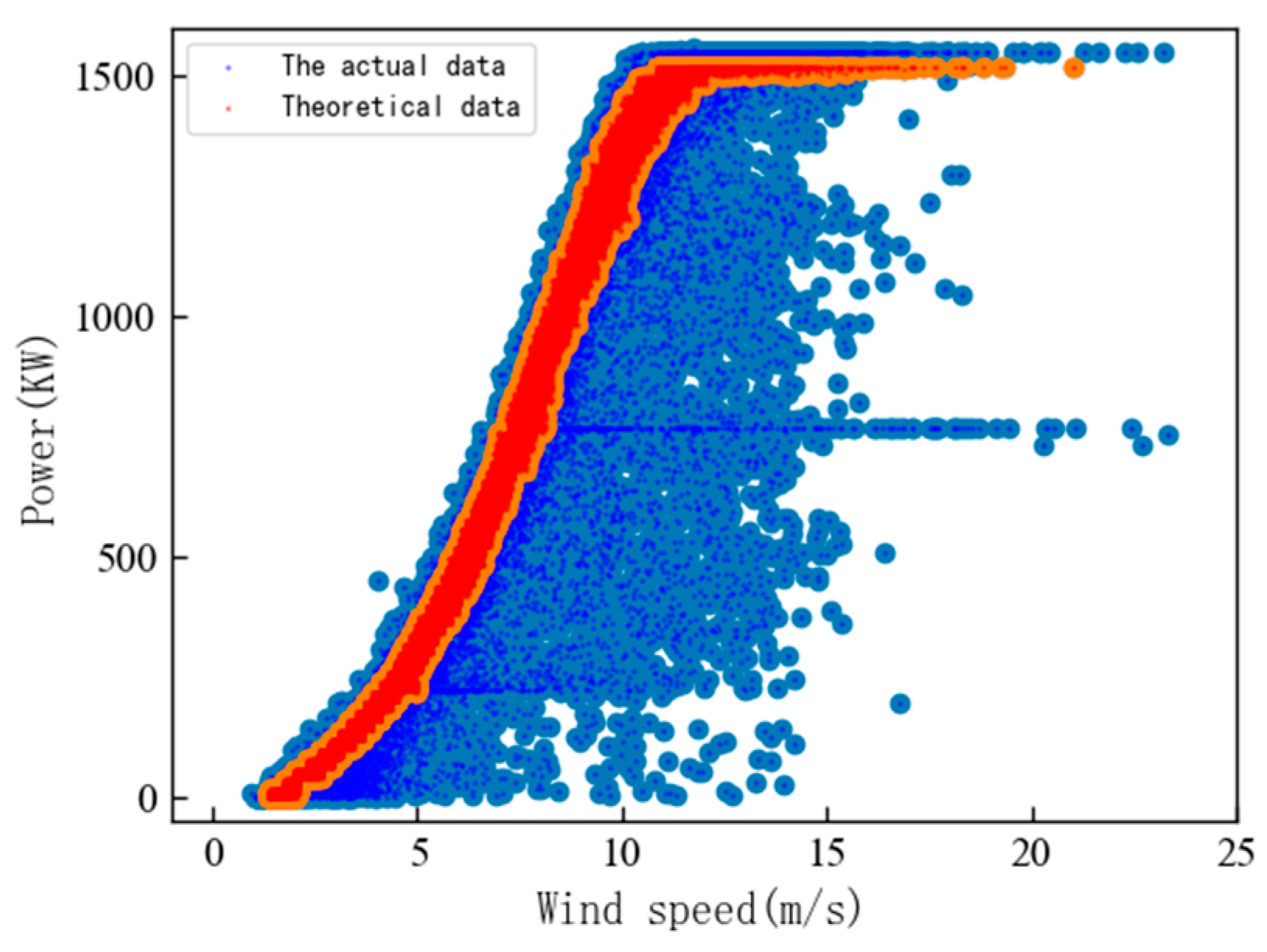
To corroborate this method’s efficacy, the wind speed data of the SDWPF wind turbine dataset over a period of one year was analyzed. The initial step involved purifying extensive historical data from the wind farm’s SCADA system, employing interpolation and clustering algorithms. The refined dataset is depicted in Figure 4, setting the stage for a comprehensive evaluation.

Figure 4. Scatter plot of 10 min wind speed–power data.

3.1.1. Modeling of Wind Power Curves

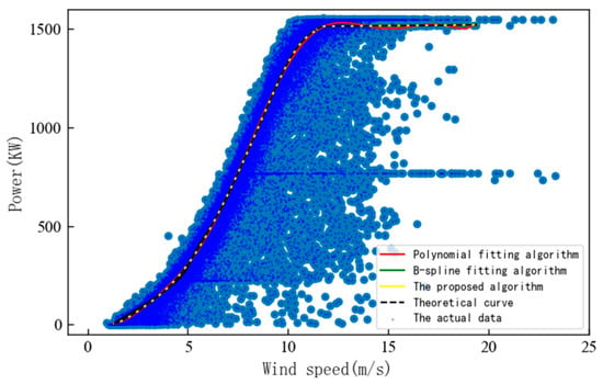
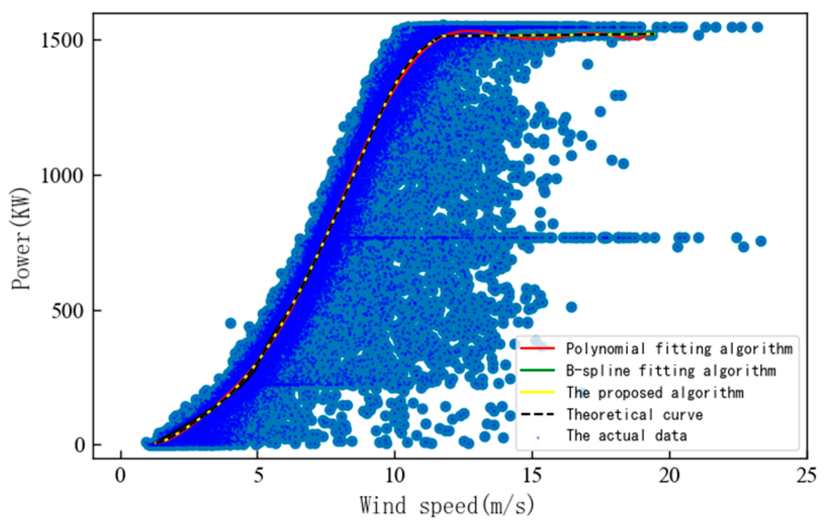
To verify the effectiveness of the proposed improved PCF algorithm, Figure 5 shows a schematic diagram of the wind turbine static optimal power curve effects constructed by the PCF algorithm, the B-spline fitting algorithm, and the algorithm of this paper.

Figure 5. Schematic diagram of optimal power curve effects.

The comparative analysis provided by the figures clearly illustrates that the polynomial fitting algorithm has a poor fitting effect on the stable curve segment after reaching the rated power. The B-spline fitting algorithm has a segment of the curve with a poor fitting effect on the rising segment of the curve from cut-in wind speed to rated wind speed, and the algorithm of this paper combines the advantages of these two algorithms, resulting in a good fitting effect on the corrected wind power data.

Table 1 provides a numerical comparison of the modeling accuracy and efficiency of the three power curve modeling algorithms.

Table 1. Comparison of curve modeling methods.

Modeling Method	NMAE	NRMSE	R2	t/s
Polynomial fitting	0.023	0.029	0.991	0.91
B-spline fitting	0.019	0.026	0.995	0.93
This article’s algorithm	0.016	0.021	0.998	0.92

Table 1 reveals that the polynomial fitting algorithm achieves a modeling accuracy of 99.1% with a fitting duration of 0.91 s. B-spline fitting offers higher accuracy, reaching up to 99.5%, but requires more time for modeling. In contrast to these two algorithms, the improved algorithm proposed in this paper increases accuracy to 99.8% while also surpassing the B-spline fitting algorithm in terms of modeling speed. Thus, the algorithm introduced in this study outperforms the polynomial and B-spline fitting algorithms in both computational efficiency and precision. Consequently, this algorithm emerges as a preferred choice for power curve modeling within practical engineering contexts, offering simplicity in concept coupled with robustness in execution speed and modeling fidelity.

3.1.2. Delineation of Wind Turbine Performance Evaluation Areas

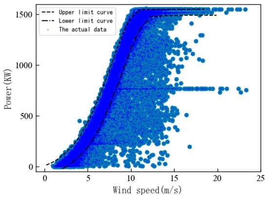
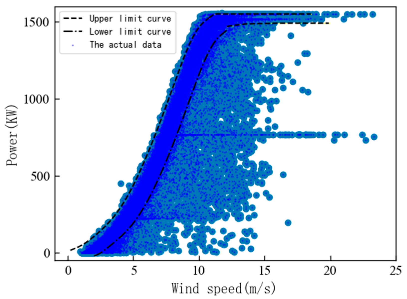
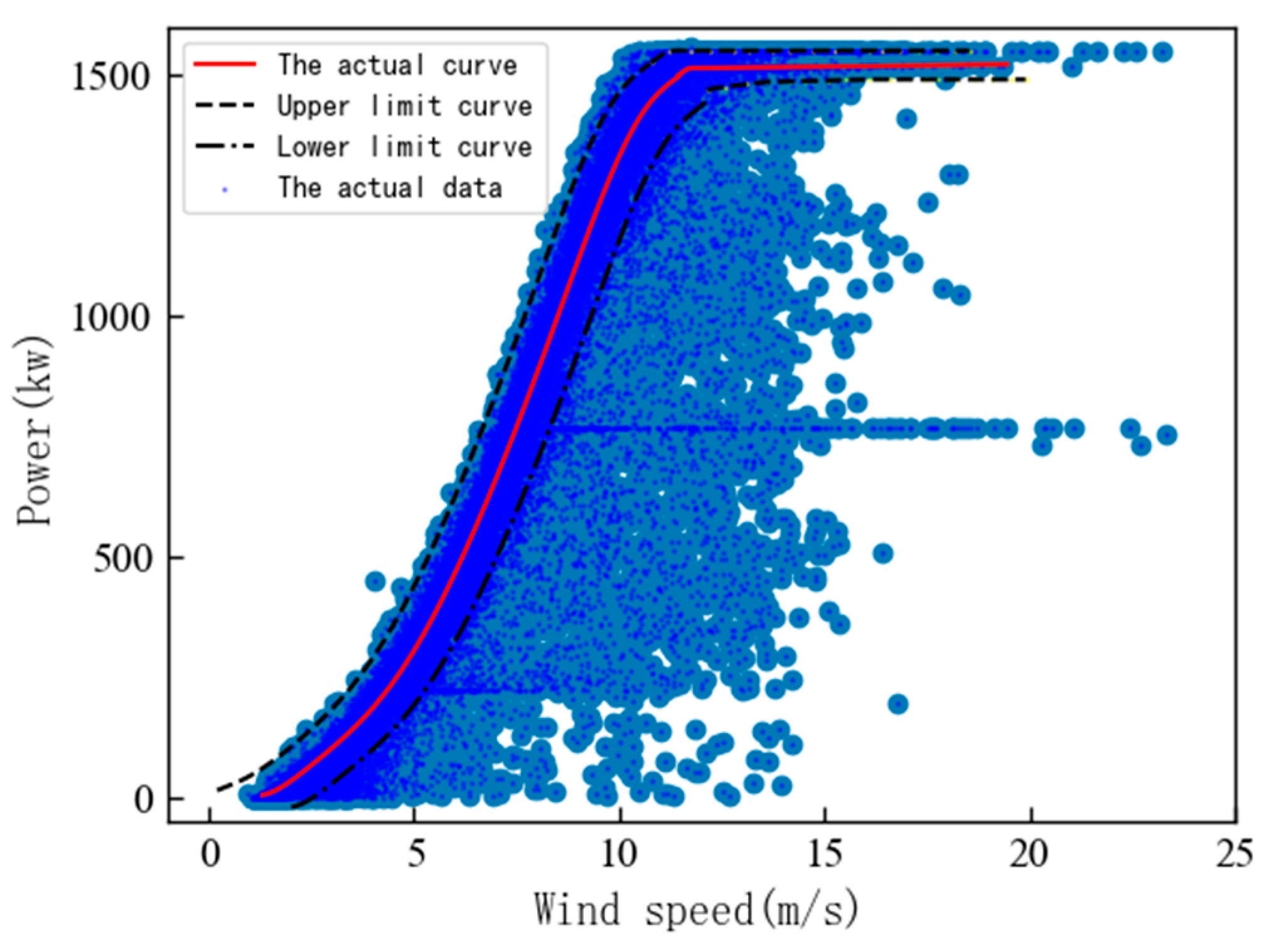
Figure 6 shows employing the optimization approach introduced in the section entitled ‘Delineation of Wind Turbine Performance Evaluation Region’, which leverages data increment inflection points, the theoretical static optimal power curve’s boundaries are ascertained. This process establishes the operational health assessment zone critical for evaluating wind turbine performance.

Figure 6. Healthy area for wind turbine performance evaluation.

Based on the determined upper and lower limit power curves of the health area, the area between the limit curves is set as the healthy zone under wind turbine operating conditions, and the area outside the healthy area is set as the abnormal zone. Analyzing the deviation of the actual power curve, there are the following situations:

• A turbine operating entirely within the healthy zone indicates normal performance status.
• If the actual power curve straddles the healthy zone and the anomaly zone, a comprehensive assessment is necessitated, factoring in indicators such as the rotational speed stability, power performance coefficient, and efficiency of power generation.

3.1.3. Wind Turbine Performance Evaluation

• Performance Evaluation Criteria

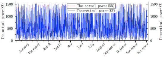
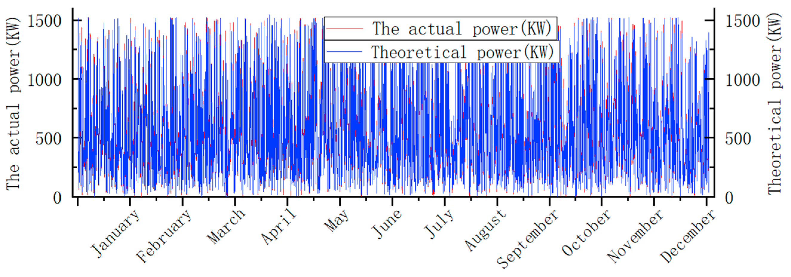
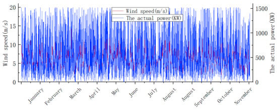
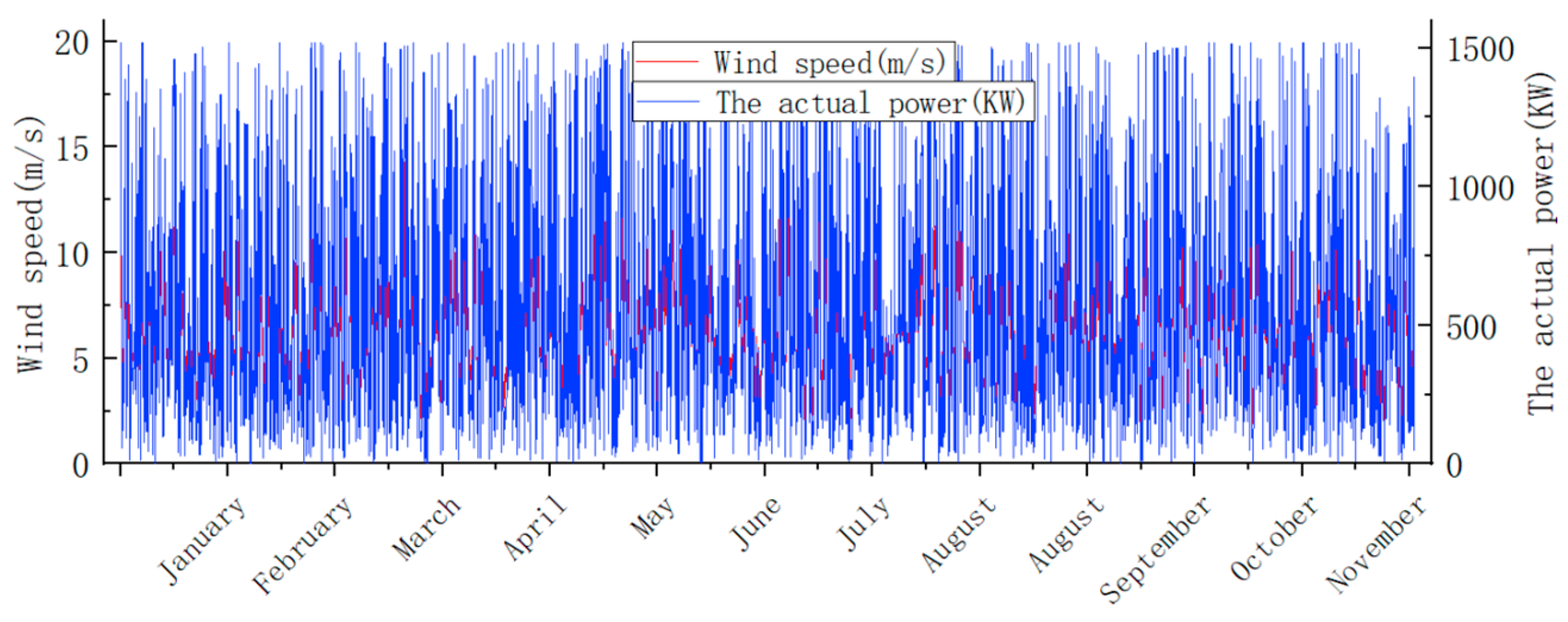
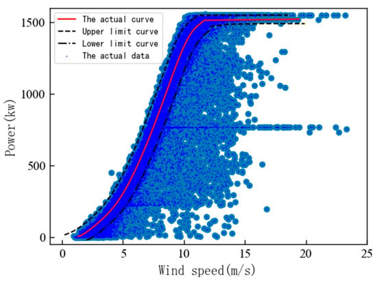
The experimental unit’s performance is extensively assessed using the criteria detailed in Section 2.2. As depicted in Figure 7, the turbine’s actual power output shows a proportional relationship with wind speed, maintaining a consistent trend.

Figure 7. Wind turbine operating status.

As depicted in Figure 8, the wind turbine’s actual power trajectory aligns closely with theoretical expectations. Notably, the power performance coefficient, as computed in Section 2.1.3, achieves an approximate value of 0.95 across various wind speed ranges $\mathrm{C}\mathrm{p}$, with the exception of the mid-range segment.

Figure 8. Wind turbine power deviation.

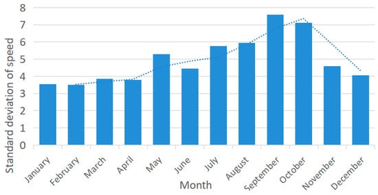
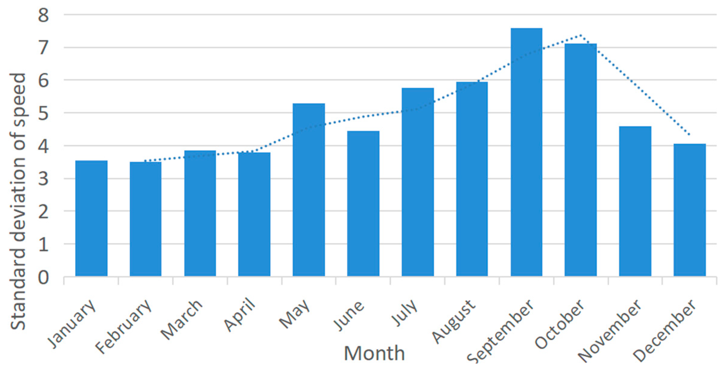
Figure 9 illustrates how summertime’s propensity for thunderstorms, heatwaves, and gusty conditions can lead to marked fluctuations in turbine rotational speeds, thereby elevating the standard deviation indicative of rotational stability.

Figure 9. Wind turbine speed stability.

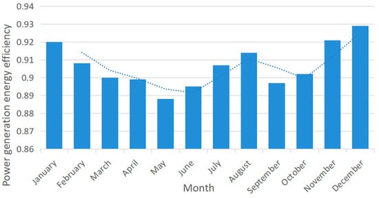
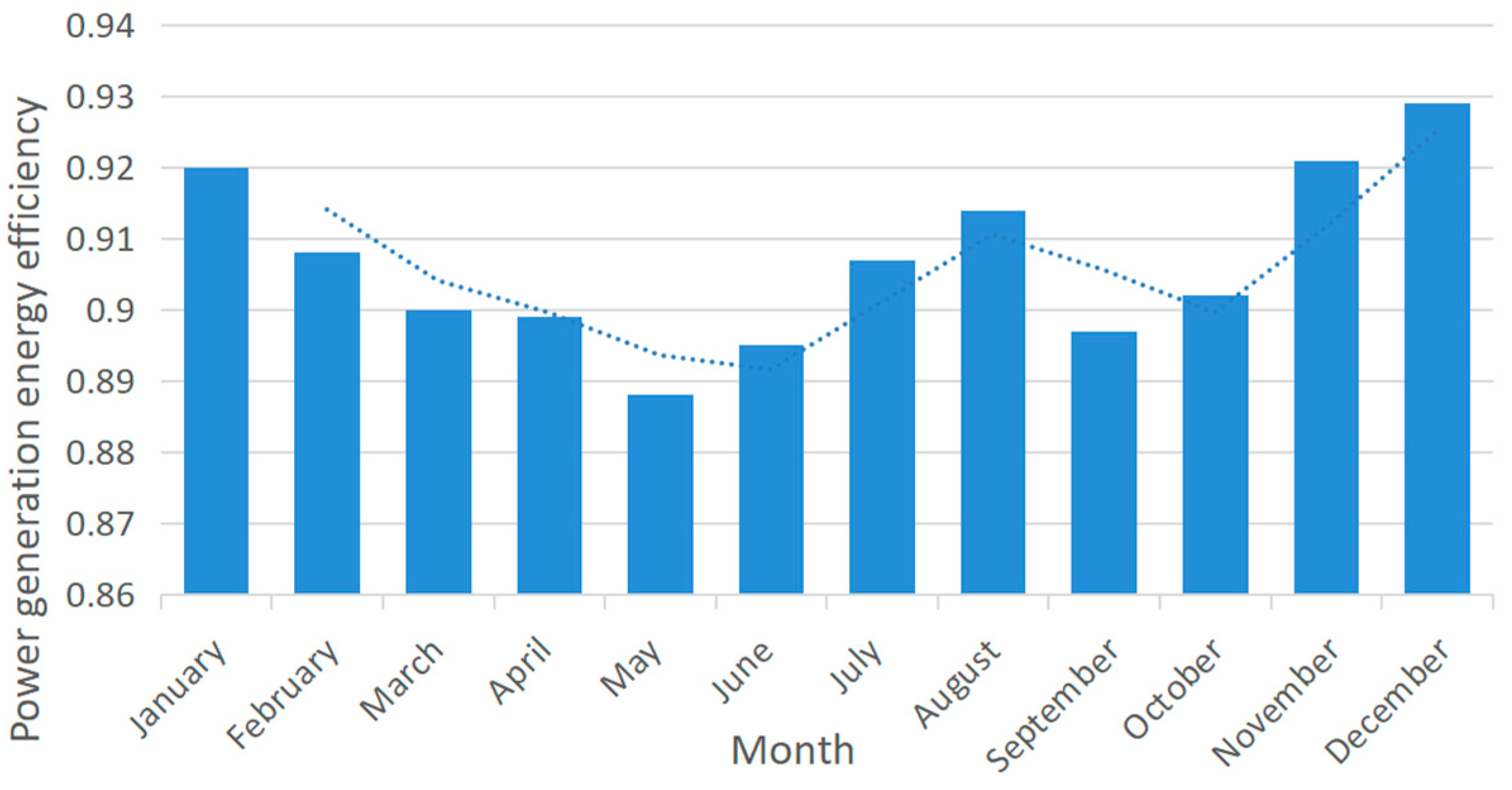
The monthly power generation efficiency graph in Figure 10 indicates an average efficiency rate of approximately 0.90608 for the unit, with peak performance observed during spring and autumn, and notably in winter.

Figure 10. Wind turbine power generation efficiency.

2.

Evaluating Wind Turbine Performance

The actual power curve of the wind turbine, depicted by the red line in Figure 11, reveals that, particularly in mid-range wind speeds, the curve approaches but does not surpass the upper boundary of the designated health zone. An in-depth analysis, incorporating the previously discussed performance metrics, uncovers a notable discrepancy between actual and theoretical power outputs in this wind speed range. This deviation, compounded by delays in the turbine control system’s response at higher wind speeds, can push the unit into an overburdened operational state. While such conditions may temporarily boost power output, they pose a risk of long-term damage to critical turbine components, including the generator, rotor system, and blades, potentially compromising the unit’s overall performance. Consequently, while the turbine’s current state is assessed as healthy, there is a discernible risk of degradation toward the anomaly zone.

Figure 11. Wind turbine actual power curve.

4. Conclusions

This study introduces a methodology that synergistically optimizes power curves and health region assessments to gauge wind turbine performance. Initial steps involve refining extensive wind power datasets through quartile analysis and MeanShift clustering. Subsequently, the enhanced power curve fitting (PCF) algorithm is employed for curve modeling, yielding the turbine’s optimal static power curve. Notably, our approach demonstrates superior modeling precision and efficiency compared to conventional PCF and B-spline methodologies. Further, this method delineates performance evaluation zones through analysis of data increment inflection points. Finally, the wind turbine’s health performance is evaluated by combining indicators such as rotational speed stability, power performance coefficient, power generation efficiency, etc. Through actual case verification, the method proposed in this paper is proven to have practical engineering significance and can be applied and promoted in wind power projects for wind turbine fault prediction and health management.

References

- Yang, M.; Dai, B. Error Analysis of Wind Speed-Power Curve Modeling in Wind Farms Based on the Binh Model. Autom. Electr. Power Syst. 2020, 40, 81–89. [Google Scholar]
- Lin, P.; Zhao, S.; Xie, Y.; Hu, Y. Modeling and Uncertainty Estimation of Wind Power Curve Based on Measured Data. Autom. Electr. Power Syst. 2015, 35, 90–95. [Google Scholar]
- Chen, S.; Guo, X.; Han, S.; Xiao, J.; Wu, N. A novel stochastic cloud model for statistical characterization of wind turbine output. IEEE Access 2020, 9, 7439–7446. [Google Scholar] [CrossRef] [Scilit]
- Zhan, Y.; Zhou, M.; Ren, D. Study and Application of Wind Turbine Power Loss Assessment based on GD-BIN Algorithm. IOP Conf. Ser. Mater. Sci. Eng. 2020, 782, 032075. [Google Scholar] [CrossRef] [Scilit]
- Chen, Z.H. Prediction of Remaining Useful Life of Electromechanical Actuators Based on Multimodal Transformer. Acta Armamentarii 2023, 44, 2920–2931. [Google Scholar]
- Xia, Q.; Lei, A.; Yan, Z.; Fenhua, L.; Hao, Z.; Jie, Y. Comparative study of multiple power curve modelling methods. Renew. Energy Resour. 2018, 36, 580–585. [Google Scholar]
- Cao, L.; Liu, W.; Guo, H. Cleaning and Modeling of Anomalous Data in Wind Farm Power Curves. J. Lanzhou Univ. Technol. 2022, 48, 64–70. [Google Scholar]
- Xu, M.; Pinson, P.; Lu, Z.; Qiao, Y.; Min, Y. Adaptive robust polynomial regression for power curve modeling with application to wind power forecasting. Wind Energy 2016, 19, 2321–2336. [Google Scholar] [CrossRef] [Scilit]
- Wang, L.; Liu, J.; Qian, F. Wind speed frequency distribution modeling and wind energy resource assessment based on polynomial regression model. Int. J. Electr. Power Energy Syst. 2021, 130, 106964. [Google Scholar] [CrossRef] [Scilit]
- Ziel, F.; Croonenbroeck, C.; Ambach, D. Forecasting wind power–modeling periodic and non-linear effects under conditional heteroscedasticity. Appl. Energy 2016, 177, 285–297. [Google Scholar] [CrossRef] [Scilit]
- Wang, F.; Liu, Y.; Cui, Q. Modeling and Optimization of Mixed-Type Parameters Based on Gaussian Process Regression. Stat. Decis. 2023, 39, 34–39. [Google Scholar]
- Liang, T.; Cui, J.; Shi, H.; Li, Z. Comparative Study on Modeling Methods of Wind Turbine Power Curve. Comput. Simul. 2021, 38, 62–66. [Google Scholar]
- Shen, X.; Fu, X. Modeling Method of Wind Turbine Power Curve Based on Improved Smooth Spline. High Volt. Eng. 2020, 46, 2418–2424. [Google Scholar]
- Zhang, P.; Xing, Z.; Guo, S.; Chen, M.; Zhao, Q. A New Wind Turbine Power Performance Assessment Approach: SCADA to Power Model Based with Regression-Kriging. Energies 2022, 15, 4820. [Google Scholar] [CrossRef] [Scilit]
- Zhan, J.; Wang, R.; Yi, L.; Wang, Y.; Xie, Z. Health assessment methods for wind turbines based on power prediction and mahalanobis distance. Int. J. Pattern Recognit. Artif. Intell. 2019, 33, 1951001. [Google Scholar] [CrossRef] [Scilit]
- Ansari, O.A.; Chung, C.Y. A hybrid framework for short-term risk assessment of wind-integrated composite power systems. IEEE Trans. Power Syst. 2018, 34, 2334–2344. [Google Scholar] [CrossRef] [Scilit]
- Zeng, T.; Liu, H.; Chen, H.; Wang, Z.; Chu, X. Wind Turbine Performance Evaluation Based on Multi-Feature Information Fusion. Comput. Integr. Manuf. Syst. 2022, 28, 1052–1061. [Google Scholar]
- Liu, Q.; Ma, H.; Chu, X.; Ma, B.; Wang, Z. Wind Turbine Performance Evaluation and Anomaly Detection Based on Long Short-Term Memory Autoencoder Neural Network. Comput. Integr. Manuf. Syst. 2019, 25, 3209–3219. [Google Scholar]
- Lin, T.; Zhang, L.; Cai, R.; Yang, X.; Liu, G.; Liao, W. Wind Turbine Performance Evaluation Based on Improved Fruit Fly Optimization Algorithm Optimized Support Vector Machine. Renew. Energy 2019, 37, 132–137. [Google Scholar]
- Li, D.; Zhang, H. Wind Turbine Performance Evaluation Based on Mutual Information Correlation of Wind Farm Big Data. Sci. Technol. Eng. 2018, 18, 211–215. [Google Scholar]
- Wan, S.; Wan, J.; Zhang, C. Wind Turbine Performance Evaluation Based on Grey Theory and Variable Weight Fuzzy Comprehensive Judgment. Acta Energiae Solaris Sin. 2015, 36, 2285–2291. [Google Scholar]
- Li, J.; Li, Y.; Wang, H.; Li, C. Health Performance Assessment and Prediction of Wind Turbine Units Based on XGBoost-Bin Automatic Power Limit Calculation [J/OL]. Computer Integrated Manufacturing Systems: 1–21. Available online: http://kns.cnki.net/kcms/detail/11.5946.tp.20220411.1552.028.html (accessed on 26 June 2024).
- Jiao, J.; Wen, Z. Assessment of Wind Turbine Performance Indicators Based on SCADA Data. Mod. Electr. Power 2020, 37, 539–543. [Google Scholar] [CrossRef]
Disclaimer/Publisher’s Note: The statements, opinions and data contained in all publications are solely those of the individual author(s) and contributor(s) and not of MDPI and/or the editor(s). MDPI and/or the editor(s) disclaim responsibility for any injury to people or property resulting from any ideas, methods, instructions or products referred to in the content. |
© 2024 by the authors. Licensee MDPI, Basel, Switzerland. This article is an open access article distributed under the terms and conditions of the Creative Commons Attribution (CC BY) license (https://creativecommons.org/licenses/by/4.0/).