A Novel Disruptive Innovation-Like Algorithm for Single-Machine Scheduling with Sequence-Dependent Family Setup Times

Abstract

This paper proposes a novel disruptive innovation-like algorithm (DILA) for the problem of scheduling a single machine with sequence-dependent family setup times to minimize the total tardiness. The proposed algorithm is derived from Christensen’s (1997) theory of disruptive innovation. Based on this theory, a DILA is proposed, which first generates two initial populations: the mainstream market population and the emerging market population. Then, to improve the quality of solutions in the populations, three phases are created within a generation. Finally, the DILA allows the populations to evolve for several generations until the termination condition is met. Two populations constructed in DILA are to overcome the weakness of premature. In addition, two functions—the member-added function and member-removed function—implemented in DILA are added to increase the diversity. The DILA was tested on a dataset of 1440 observations from the literature. The computational results confirm that DILA is very effective.

1. Introduction

In this paper, a novel disruptive innovation-like algorithm (DILA) is proposed for solving the single-machine scheduling problem with sequence-dependent family setup times (SMSDFS) to minimize the total tardiness. The candidate scheduling problem can be found in real-life manufacturing environments, such as the module process in Thin film transistor liquid crystal display (TFT LCD) manufacturing [1] and steel wire factories [2,3]. In addition, the considered SMSDFS problem is also suitable for evaluating the performance of the DILA. This is because the single-machine scheduling problem can be used as the basis for the development of heuristics [4].

The concept of the proposed DILA was mainly derived from Christensen’s [5] theory of disruptive innovation. Disruptive innovation divides the market into a mainstream and an emerging market. The price and quality of the products offered by companies within the mainstream market are higher, which is not accepted by all consumers. Hence, another group of companies introduces disruptive innovation products into the emerging market to attract those consumers who do not accept the products offered in the mainstream market. Consumers in the emerging market have no choices other than the disruptive innovation products. However, with the improvement of the quality of the low-end products, mainstream consumers, who are more fastidious about the quality of products, also move away from the original value network to enter this emerging market. This also means that companies in the mainstream market that focus on the provision of high-end products cannot grow after a period of time. Thus, the emerging market gradually becomes a mainstream market. In addition, the companies in the emerging market will continue to self-develop and grow their business evolution and development processes as well as imitate the management approach of the companies with outstanding performance. Some companies will exit the market because of certain factors leading to business failure, while new companies will also join the market.

The theory of disruptive innovation includes two markets: the mainstream market and the emerging market. The two markets used in DILA represent two populations: the mainstream market population and the emerging market population. Therefore, the DILA can be regarded as a kind of population-based algorithm. Previous studies on the development of algorithms, such as genetic algorithms, particle swarm optimization algorithms, and ant colony optimization algorithms, usually consider only one population. There are many members in each population, with each member representing a company. In other words, each company is a member, which is a solution, while the profitability performance of companies represents the quality of the solutions. There is a “co-opetition” relationship between companies, which allows them to learn from each other and to put more effort into moving toward profitability. In addition, members with poor performance may be eliminated from the population, and new members can be added to the population.

Even without setup considerations, the single-machine total tardiness problem is proven to be NP-hard (non-deterministic polynomial-time hardness) [6], so the candidate problem is a NP-hard problem as well. It requires much computational time to find the optimal solution. Therefore, the development of heuristics that find near-optimal solutions in a reasonable amount of computational time has attracted the attention of many researchers in recent decades. The SMSDFS problem has been solved by several research studies. Baker [7] examines heuristic solution procedures for scheduling jobs on a single machine to minimize the maximum lateness in the presence of setup times between different job families. Jin et al. [2] develop a tabu search and Jin et al. [3] present a simulated annealing algorithm to solve the SMSDFS problem of minimizing maximum lateness. Hinder and Mason [8] present a novel integer-programming formulation for scheduling with family setup times on a single machine to minimize maximum lateness. The authors use the branch-and-bound and integer program to find optimal schedules for significantly larger problem instances such as the problems with 1080 jobs and 270 families. Jacob and Arroyo [9] developed three heuristics based on the iterated local search (ILS) metaheuristic to solve SMSDFS for minimizing total tardiness. The first heuristic is a basic ILS (ILS_BASIC), the second employs a dynamic perturbation size (ILS_DP), and the third uses a path relinking (PR) technique as an intensification strategy (ILS_DP + PR). The authors use these three heuristics, ILS_BASIC, ILS_DP, and ILS_DP + PR, and the HGA (hybrid genetic algorithm) [10] to obtain solutions for a set of 1440 benchmark instances. These benchmark instances are also used to access the performance of the proposed DILA.

The remainder of this paper is organized as follows: Section 2 provides a detailed description of the problem, Section 3 describes the proposed algorithms, Section 4 presents the computational experiments and reports the results, and Section 5 concludes the paper.

2. Description of the Problem

The scheduling problem considered in this study can be described as follows: A set of independent jobs $J_i$ ($i=1,2,\dots ,n$) has to be scheduled on a single machine without interruption or preemption. All the jobs are available for processing at time zero, machine breakdown does not occur, and the machine can process only one job at a time. Each job $J_i$ has a positive processing time $p_i$ and a due date $d_i$. Jobs are classified into F families. Each family l has $n_l$ jobs $\left(l=1,2,\dots ,F\right)$ such that $n_1+n_2+\dots n_F=n$. (i) denotes the family of job i. Here, the family setup time, $s_{ij}$, is determined by job j that is scheduled to be performed after job i by the machine, with $f\left(i\right)\ne f\left(j\right)$. If jobs i and j belong to the same family $\left(f\left(i\right)=f\left(j\right)\right)$, there is no setup time, that is, $s_{ij}$ is zero. The following notations are used to describe the SMSDFS problem and the proposed DILA in the next section:

• i = job index, i = 1,2,3,…,n
• $p_i$= processing time of job i
• l = family index, l = 1,2,3,…,F
• (i) = the family of job i
• $s_{ij}$ = family sequence-dependent setup time of job j is processed immediately after job i
• $d_i$= due date of job i
• P1 = population 1
• P2 = population 2
• P_num1 = the number of members in P1
• P_num2 = the number of members in P2
• ${\Pi }_{1p}$ = the solution p in P1
• ${\Pi }_{2p}$ = the solution p in P2
• ${\Pi }^{gbest}$ = the best solution in P1 and P2
• ${\Pi }_1^{lbest}$ = the local best solution in P1
• ${\Pi }_2^{lbest}$ = the local best solution in P2
• $V_{1p}$ = the value of the member p in P1
• $V_{2p}$ = the value of the member p in P2
• $V_1^{lbest}$ = the value of the local best solution in P1
• $V_2^{lbest}$ = the value of the local best solution in P2
• $V^{gbest}$ = the value of the global best solution in P1 and P2
• ${\Pi }^{VND}$ = the solution generated by variable neighborhood descent (VND) algorithm
• $V^{VND}$ = the value of the solution generated by VND algorithm
• $c1,c2$ = the values for controlling the probabilities of executing the member-added function and member-removed function
• C_i = completion time of job i
• T_i$=\{\begin{array}{c}\begin{array}{cc}\left(C_i-{\mathrm{d}}_i\right)& \end{array}\mathrm{if}\left(C_i-{\mathrm{d}}_i\right)>0,\\ 0\mathrm{otherwise}.\end{array}$

The scheduling problem considered in this paper is to minimize the total tardiness. The objective can be defined as below:

Objective = Minimize ${{\displaystyle \sum }}_{i=1}^n{T}_i$.

3. Proposed Algorithm

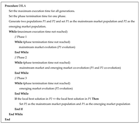
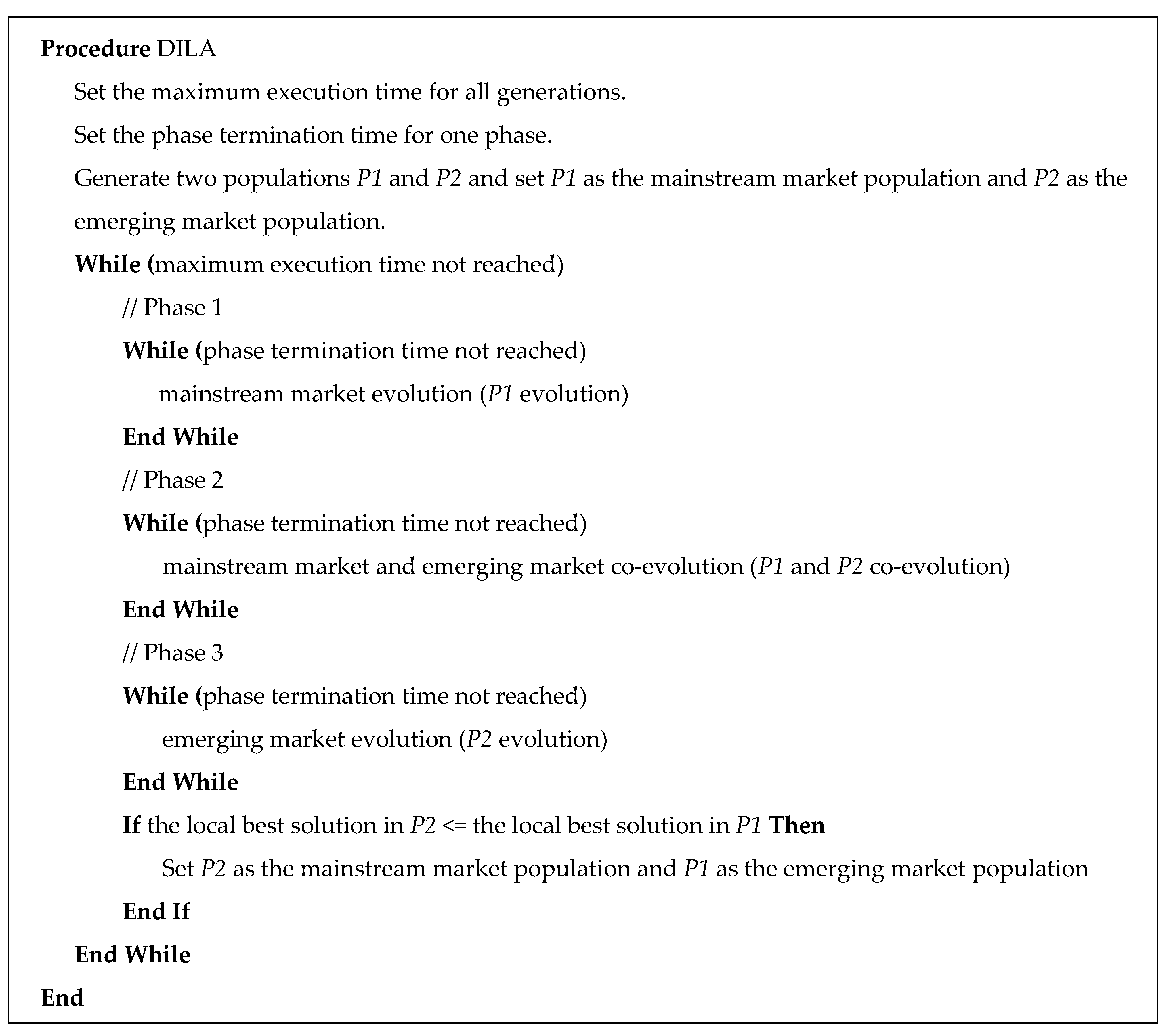
In this paper, a novel DILA is proposed to solve the candidate problem. The main components of the DILA include the initialization of the populations and the three-phase evolution, namely, the mainstream market evolution, mainstream and emerging market co-evolution, and emerging market evolution. In the first phase of the DILA, only the mainstream market population evolves; the emerging market population does not exist in this first phase of evolution. In the second phase of the DILA, the emerging market population joins the second phase of evolution, and the mainstream market population and the emerging market population evolve at the same time. The members of both the mainstream market population and the emerging market population can learn from the local best solution or the global best solution. In the last phase, only the emerging market population is evolving. In the DILA, the three phases are repeated until the termination condition is met. The three phases can be regarded as one generation. After the end of one generation, it is judged which population has a better solution, and then that population becomes the mainstream market population in the next generation. Figure 1 illustrates the basic process of the DILA, and the main components of the proposed DILA are described below.

Figure 1. Basic process of the proposed disruptive innovation-like algorithm (DILA).

3.1. Initial Populations

As mentioned above, the DILA includes two populations. The first population’s members are generated by two heuristics: the apparent tardiness cost with setup (ATCS) rule [11] and the destruction and construction (DC) procedure [12]. The second population’s members are generated by the RANDOM rule and the DC procedure. The priority of the ATCS rule used in the paper can be expressed as follows:

$$I_i\left(t,j\right)=\frac{1}{p_i}\exp \left[-\frac{\max (d_i-p_i-t,0)}{k_1\overline{p}}\right]\exp \left[-\frac{s_{j,i}}{k_2\overline{s}}\right],$$

where t denotes the current time; job j has just been completed on the machine; $\overline{p}$ and $\overline{s}$ represent the average processing time and average setup time of all remaining jobs, respectively; k₁ and k₂ are look-ahead or scaling parameters. Values of k₁ = 4.75 and k₂ = 0.15 are used in the paper.

The generation method for the first population’s members works as follows: The ATCS rule is used to generate a member solution. Then, based on the generated member solution, the DC procedure is used to regenerate P_num1 different solutions, where P_num1 is the size of population 1. The main difference between the generation mechanism for the first and second population’s members is that the generated solution from the second population uses the RANDOM rule to randomly generate a solution. Based on the generated member solution, the DC procedure is used to regenerate P_num2 different solutions, where P_num2 is the size of population 2.

We calculate the objective value for each member of each population. The population that has the best solution is set as the mainstream market population (P1), and the other one is set as the emerging market population (P2).

3.2. Evolution of the Mainstream Market Population

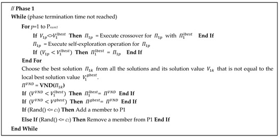
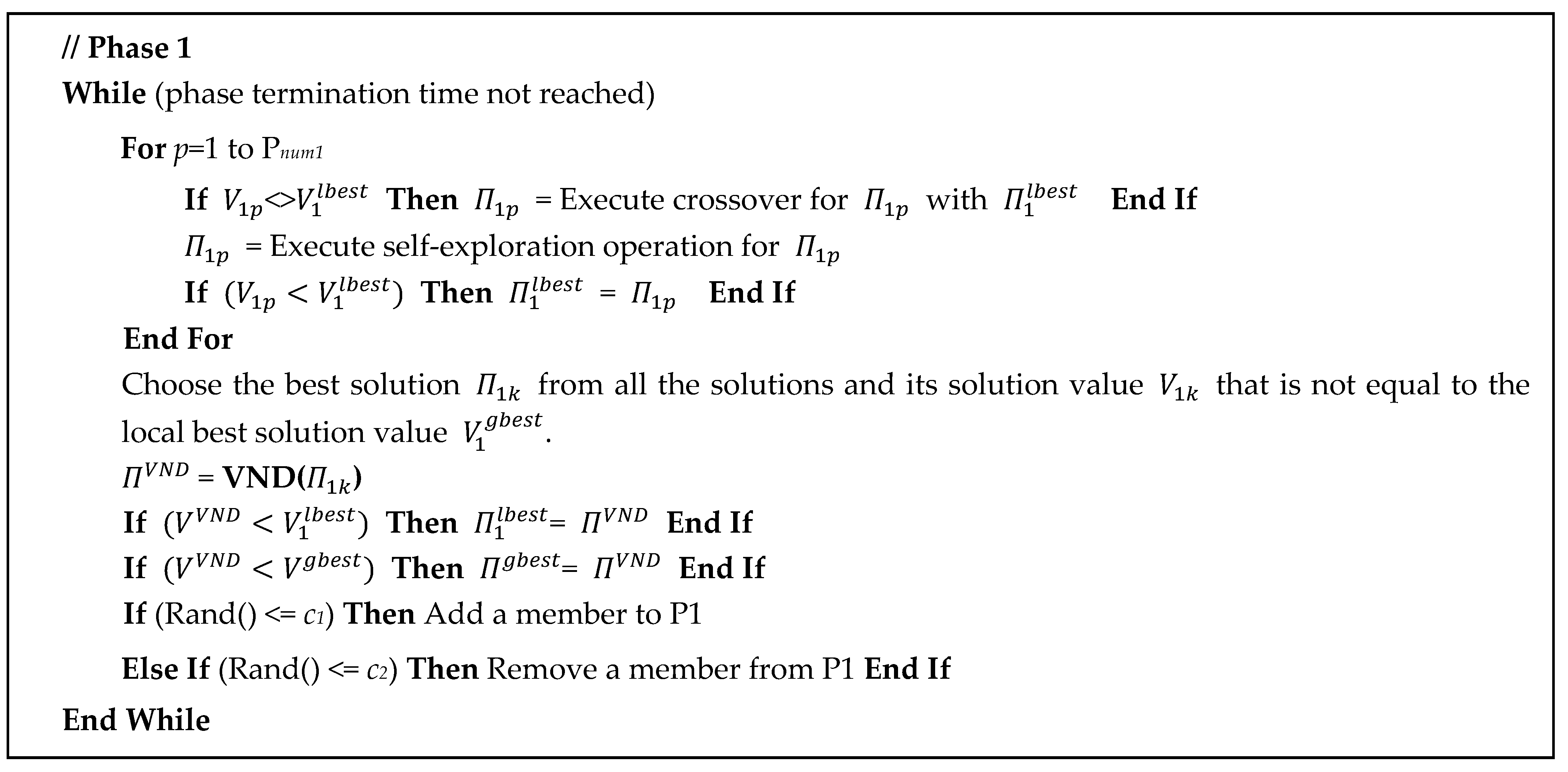
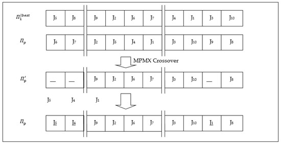
In the DILA, the mainstream market population evolves first (phase 1). The procedure for the evolution of the mainstream market population is presented in Figure 2. The members of the population will be updated by using two methods: (1) learning from the local best solution and (2) self-learning. The partially mapped crossover (PMX) operator suggested by Goldberg and Lingle [13] is modified to be the learning method in the paper. For convenience, we named it MPMX. It allows an information exchange between member p (${\Pi }_{1p}$) and the local best solution ${\Pi }_1^{lbest}$ when the member’s solution value ($V_{1p}$) is not equal to the local best solution value ($V_1^{lbest}$). The MPMX crossover used in this study is described as follows. Taking Figure 3 as an example, there are two members with 10 jobs between them in the diagram, namely, member ${\Pi }_{1p}$ and the local best solution ${\Pi }_1^{lbest}$. The member ${\Pi }_{1p}$ can inherit a fixed length of subsequence from the local best solution ${\Pi }_1^{lbest}$. We assumed that the fixed length is 4 and one point was selected randomly is 3, for example, positions 3 and 6, which indicated that member ${\Pi }_{1p}$ would inherit the jobs in positions 3 to 6 from the local best solution ${\Pi }_{1p}$. The rest of the positions in ${\Pi }_p$, such as J₃, J₁₀, and J₈, were retained if they were not the same as the inherited jobs in positions 3 to 6. The order of the repetitive parts, such as J₅, J₄, and J₁, were determined by the original order of member ${\Pi }_{1p}$. Then, they were filled into the blank positions 1, 2, and 9 in sequence from left to right. Then, J₅ is first placed into the blank position; when all the jobs are put into the blank positions, a new individual solution ${\Pi }_p$ is formed. Furthermore, the DC procedure [12] is applied as the self-learning method.

Figure 2. The procedure for the evolution of the mainstream market population in the DILA.

Figure 3. The modified partially mapped crossover operator (MPMX).

When all members in population 1 have been updated, a solution ${\Pi }_{1k}$ is selected, and the variable neighborhood descent (VND) algorithm is used to improve the solution. The selected solution value $V_{1k}$ is the minimum among all the members’ solution values and is different from the local best solution value $V_1^{lbest}$. The VND is a metaheuristic proposed by Hansen and Mladenović [14] has been successfully applied to solve scheduling problems. The VND searches the solution space using a set of predefined neighborhood structures. The search escapes from local optima by systematically changing these neighborhood structures. In the paper, a series of neighborhood structures based on the insertion move of a subsequence (block) is implemented as the neighborhood structures of the VND. The variable sequence of neighborhood structures used in this paper is the same as the one in Chen [15], which employs eight insertion neighborhood structures. The move of a subsequence may involve a one-job insertion move, two consecutive jobs insertion move, …, or eight consecutive jobs insertion move. For convenience, a one-job insertion move is denoted as INS(1), a two consecutive jobs insertion move is denoted as INS(2), …, and the eight consecutive jobs insertion move is denoted as INS(8).

Finally, two functions—the member-added function (MAF) and member-removed function (MRF)—are implemented to represent the joining and disappearance of members. A new member is added to the population, or a member of the population is eliminated according to two controlled parameters, c₁ and c₂, which are less than or equal to 1.0. The values c₁ and c₂ are set in order to generate competent probabilities that preserve population diversification. Eleven combinations of c₁ and c₂ shown in Table 1 are considered in this paper. The probability values p_a and p_r for each of the combinations are calculated as follows. First, c₁ is used to determine p_a (p_a = c₁), and c₂ is used to determine p_r (p_r = (1 − c₁) × c₂). For instance, if c₁ = 0.2 and c₂ = 0.25 (the second combination in Table 1), then p_a = c₁ = 0.2 and p_r = (1−c₁) × c₂ = 0.2.

Table 1. The eleven combinations of c₁ and c₂ considered in member-added function (MAF) and member-removed function (MRF).

Controlled Parameters		Controlled Probability
c1	c2	pa	pr
0	0	0.0	0.0
0.2	0.25	0.2	0.2
0.2	0.5	0.2	0.4
0.2	0.75	0.2	0.6
0.2	1	0.2	0.8
0.5	0.4	0.5	0.2
0.5	0.8	0.5	0.4
0.5	1	0.5	0.5
0.8	1	0.8	0.2
1	0	1.0	0.0
0	1	0.0	1.0

The values of p_a and p_r for the combinations in Table 1 demonstrate the purpose of selecting the 11 combinations. A combination with a larger p_a and a smaller p_r implies that the probability that a member will be added is larger than the probability that a member will be removed. On the contrary, for a combination with a smaller p_a and a larger p_r, the probability that a member will be removed is larger than the probability that a member will be added. The first combination (c₁ = 0.0 and c₂ = 0.0) is used for the case where no member is added or removed. The last two combinations (c₁ = 1.0 and c₂ = 0.0, and c₁ = 0.0 and c₂ = 1.0) are used for the cases where a member is always subjected to the MAF (p_a = 1.0) or the MRF (p_a = 0.0 and p_r = 1.0), respectively.

The MAF is implemented with a probability of p_a; this function randomly generates a solution and applies the DC procedure to shake it and then adds it to the population. The MRF is implemented with a probability of p_r; this function eliminates the member with the worst objective value. This search process of the phase continues until a phase termination criterion is satisfied.

To increase the diversity of the population, the two-stage MAF and MRF mechanism is proposed. This two-stage mechanism means that in the first half of all the execution time, we use a set of control probability and then use another set of control probability in the last half of the execution time to do MAF and MRF.

3.3. Co-Evolution of Mainstream Market Population and Emerging Market Population

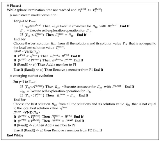
After the mainstream market evolution, the emerging market members join the evolution (phase 2), namely, the co-evolution. The procedure for the co-evolution of the mainstream market and the emerging market is presented in Figure 4. The members in the mainstream and emerging market populations learn from the global best solution and engage in self-learning. The MPMX crossover operator, DC procedure, MAF, and MRF used in phase 1 are also used in phase 2. However, in phase 2, the learning method allows information to be exchanged between a member and the global best solution ${\Pi }^{gbest}$ when the member’s solution value is not equal to the global best solution value. Members of the emerging market population can also learn from the global best solution. This is because the emerging market companies can refer to the practices of the mainstream market companies that already exist. This search process of the phase continues until a phase termination criterion is satisfied or the local best solution of the emerging market population ($V_2^{lbest}$) is better than the local best solution of the mainstream market population ($V_1^{lbest}$). If $V_2^{lbest}$ is smaller than $V_1^{lbest}$, the profitability of the emerging market has surpassed that of the mainstream market. Therefore, phase 2 can be terminated and phase 3 begins, in which only the emerging market evolves.

Figure 4. The procedure for the co-evolution of the mainstream and emerging market populations in the DILA.

3.4. Evolution of Emerging Market Population

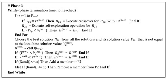
In phase 3, only the emerging market population evolves. The procedure for the evolution of the emerging market population is presented in Figure 5. The members in the emerging market population will learn from the global best solution and engage in self-learning. The MPMX crossover operator, DC procedure, MAF, and MRF used in phase 2 are also used in this phase.

Figure 5. The procedure for the evolution of the emerging market population in the DILA.

4. Computational Experiments

To verify the performance of the proposed DILA, two sets of experiments were conducted. The first set investigates the effects of the controlled probability and the phase termination time. The second set compares the performance of the DILA with the best parameters found in the first set against several metaheuristics reported in the literature.

We coded the DILA in C++ and executed it on an Intel Core i7 PC with a 3.4 GHz CPU and 4 GB RAM. A series of computational experiments were conducted to compare the results of all the combinations of the algorithms with the benchmark instances provided by Jacob and Arroyo [9]. The problem instances are characterized by four factors: the number of jobs n, number of families F, due-date range r, and setup-time range η. The number of jobs has three levels, which are set at 60, 80, and 100. The number of families has four levels, which are set at 2, 3, 4, and 5. The due date of jobs is generated from integer numbers uniformly distributed in the interval $\left[0,r{{\displaystyle \sum }}_{j=1}^n{p}_j\right]$ (recall that r is the due-date range). The due-date range r has four levels: 0.5, 1.5, 2.5, and 3.5. Three setup-time ranges η—[11, 20], [51, 100], and [101, 200]—are used to generate job setup times. The processing time for a job is generated from a discrete uniform distribution [1, 99]. From each of the 144 combinations of the four factors, 10 problem instances, each involving a processing time in the interval [1, 99], were generated. Therefore, a total of 1440 instances were used to evaluate the proposed algorithms.

The relative deviation index (RDI) and number of best solutions (NBS) produced are the two criteria used to evaluate the performance of the proposed algorithms. The RDI is calculated as follows:

$$\mathrm{RDI}\%=100\times \{\begin{array}{c}\begin{array}{cc}\frac{S_a-S_b}{S_w-S_b}& \end{array}\mathrm{if}\left(S_w-S_b\right)\ne 0,\\ 0\mathrm{otherwise}.\end{array}$$

Sa is the solution obtained by method a, and S_b and S_w are the best and the worst solution values, respectively, among the solutions obtained by all the methods included in the comparison.

4.1. The First Set of Experiments

For the first set of experiments, six instances (instances 506, 709, 781, 809, 897, and 909) with 80 jobs were used to investigate the effects of the parameters. The parameter of controlled probability has 17 separate levels (see Table 2). The single-stage type has 11 levels, and the two-stage type has six levels. The parameter of the phase termination time has three levels: 1, 2, and 3 s. Therefore, there are a total of 51 different combinations of the two major parameters. The remaining parameters of the DILA were set as follows: the fixed length for the MPMX crossover was set to 15, the DC size for the DC procedure was set to 4, the neighborhood structure was set to INS(1) + INS(2) + … + INS(8), the initial population size was set to 30, and the maximum execution time was set to 40 s. Then, the DILA was applied to each of the 51 combinations to solve the six instances five times each.

Table 2. The values of the controlled probability.

Type of MAF and MRF	Controlled Probability $({\mathit{p}}_{\mathit{a}},{\mathit{p}}_{\mathit{r}})$
Single Stage	(0.00, 0.00) (0.20, 0.20) (0.20, 0.40) (0.20, 0.60) (0.20, 0.80) (0.50, 0.20) (0.50, 0.50) (0.50, 0.50) (0.80, 0.20) (1.00, 0.00) (0.00, 1.00)
Two Stage	Stage 1= (0.20, 0.20), stage 2 = (0.50, 0.20) Stage 1= (0.20, 0.20), stage 2 = (0.80, 0.20) Stage 1= (0.50, 0.20), stage 2 = (0.20, 0.20) Stage 1= (0.50, 0.20), stage 2 = (0.80, 0.20) Stage 1= (0.80, 0.20), stage 2 = (0.20, 0.20) Stage 1= (0.80, 0.20), stage 2 = (0.50, 0.20)

Analysis of variance (ANOVA) was used to analyze the RDI produced by the DILA runs of all the 51 combinations for the six instances. Table 3 presents the results of the ANOVA, showing that the parameter of controlled probability significantly affects the performance of the DILA. Therefore, we applied Duncan’s test to test if the performance of any two controlled probabilities is significantly different. Table 4 presents the results of Duncan’s test. Note that the different letters indicate the performance of the DILA with the indicated levels being significantly different. The results in Table 4 show that the following combinations of the controlled probabilities produce the best mean RDI: stage 1: ($p_a^1=0.5$, $p_r^1=0.2$); stage 2: ($p_a^2=0.8$, $p_r^2=0.2$). Furthermore, the results show that the single-stage type produces the six worst mean RDIs. Table 3, the ANOVA table, also shows that the phase termination time does not significantly affect the output. This means that the three levels do not affect the DILA differently. However, the phase termination time of 2 s produces the best mean RDI. Based on the results, these analyses suggest that the best parameters are as follows: controlled probability: stage 1 = (0.50, 0.20) and stage 2 = (0.80, 0.20) and phase termination time: 2 s.

Table 3. ANOVA table for testing the significance of the major parameters of DILA.

Source	Type III Sum of Squares	df	Mean Square	F	Sig.
Corrected model	20.936 a	23	0.91	76.385	0
Intercept	19.095	1	19.095	1602.365	0
Instances	20.603	5	4.121	345.773	0
Controlled probability	0.328	16	0.02	1.719	0.043
Phase termination time	0.006	2	0.003	0.238	0.788
Error	3.361	282	0.012
Total	43.392	306
Corrected total	24.297	305

^a: R Squared = 0.862 (Adjusted R Squared = 0.850).

Table 4. Results of Duncan’s multiple range test for the controlled probability (α = 0.05).

Controlled Probability $({\mathit{p}}_{\mathit{a}},{\mathit{p}}_{\mathit{r}})$	Results (Groups)	Average RDI
stage 1 = (0.50, 0.20), stage 2 = (0.80, 0.20)	A	0.2098
(0.20, 0.80)	A	0.2179
(0.20, 0.60)	A	0.2183
stage 1 = (0.50, 0.20), stage 2 = (0.20, 0.20)	A	0.2190
(0.50, 0.20)	A	0.2213
stage 1 = (0.20, 0.20), stage 2 = (0.50, 0.20)	A	0.2232
stage 1 = (0.80, 0.20), stage 2 = (0.20, 0.20)	A	0.2259
stage 1 = (0.80, 0.20), stage 2 = (0.50, 0.20)	A	0.2450
(1.00, 0.00)	A	0.2454
(0.00, 1.00)	AB	0.2492
stage 1 = (0.20, 0.20), stage 2 = (0.80, 0.20)	AB	0.2556
(0.50, 0.50)	AB	0.2582
(0.80, 0.20)	AB	0.2618
(0.20, 0.20)	AB	0.2759
(0.50, 0.50)	AB	0.2935
(0.00, 0.00)	AB	0.2958
(0.20, 0.40)	C	0.3309

4.2. The Second Set of Experiments

The second set of experiments investigated the performance of the DILA using the best parameter values determined in the first set of experiments. We compared the performance of the proposed DILA with four heuristics [9]: HGA, ILS_BASIC, ILS_DP, and ILS_DP + PR. The results of the four heuristics are provided by Jacob and Arroyo [9]. For a fair comparison of these algorithms, 30 runs of the DILA were intentionally performed with a time limit of n*0.5 s for 1440 test instances, which is in the same stop condition as in Jacob and Arroyo [9].

Table 5 lists the RDI and NBS for different job and family sizes obtained by the DILA and the four heuristics. There are 120 instances per n × F group. The results in Table 5 show that the DILA was able to find the best solutions for 1435 out of 1440 instances (99.7%). The average RDIs show that the DILA dominated HGA by 98.3% ((17.96 − 0.3)/17.96), dominated ILS_BASIC by 91.0% ((3.34 − 0.3)/3.34), dominated ILS_DP by 87.3% ((2.37 − 0.3)/2.37), and dominated ILS_DP + PR by 80.0% ((1.50 − 0.3)/1.50). Table 6 presents the results of the paired t-tests for HGA, ILS_BASIC, ILS_DP, ILS_DP + PR, and the DILA. The results show that the DILA dominates HGA, ILS_BASIC, ILS_DP, and ILS_DP + PR at a significance level of 0.05. A comparison with the reference heuristics is summarized in Table 7, where the number of solutions better than, equal to, and worse than those obtained by the DILA are presented. We observe that the DILA outperformed HGA, ILS_BASIC, ILS_DP, and ILS_DP + PR. Compared with HGA, ILS_BASIC, ILS_DP, and ILS_DP + PR, the proposed DILA produced 258, 113, 105, and 68 better solutions, respectively, for the 1440 instances, whereas the number of worse solutions did not exceed 4.

Table 5. Relative deviation index (RDI) and number of best solutions (NBS) of the HGA, ILS_BASIC, ILS_DP, and ILS_DP + PR, and DILA heuristics.

n × F	HGA	ILS_BASIC	ILS_DP	ILS_DP + PR	DILA
60 × 2	0.83/119	0.00/120	0.00/120	0.00/120	0.00/120
60 × 3	0.83/119	0.00/120	0.00/120	0.00/120	0.00/120
60 × 4	5.00/114	0.00/120	0.83/119	0.00/120	0.00/120
60 × 5	6.67/112	1.25/118	0.40/119	0.06/119	0.00/120
80 × 2	5.00/114	1.67/118	1.25/118	0.00/120	0.00/120
80 × 3	12.26/105	1.67/118	1.83/117	0.00/120	0.83/119
80 × 4	24.87/89	3.87/110	5.47/111	2.21/114	0.83/119
80 × 5	30.53/83	3.36/109	2.88/111	5.22/111	0.00/120
100 × 2	17.37/99	5.24/112	0.55/115	0.00/120	0.00/120
100 × 3	31.68/81	7.11/97	3.25/101	2.41/111	0.28/119
100 × 4	39.81/72	7.77/94	6.28/93	3.45/106	1.67/118
100 × 5	40.72/71	8.15/88	5.65/87	4.70/91	0.00/120
Average	17.96/1178	3.34/1324	2.37/1331	1.50/1372	0.30/1435

Table 6. Paired t-test for HGA, ILS_BASIC, ILS_DP, and ILS_DP + PR, and DILA heuristics.

		Paired Differences					t	df	Sig. (2-Tailed)
		Mean	Std. Deviation	Std. Error Mean	95% Confidence Interval of the Difference
					Lower	Upper
Pair 1	HGA–DILA	17.66	38.02	1.00	15.70	19.63	17.63	1439	0.00
Pair 2	ILS_BASIC–DILA	3.04	15.70	0.41	2.23	3.85	7.35	1439	0.00
Pair 3	ILS_DP–DILA	2.06	12.77	0.34	1.40	2.72	6.14	1439	0.00
Pair 4	ILS_DP + PR–DILA	1.20	11.22	0.30	0.62	1.78	4.07	1439	0.00

Table 7. Summary of comparing DILA with reference heuristics.

	HGA	ILS_BASIC	ILS_DP	ILS_DP + PR
Number of improved solutions	258	113	105	68
Number of equal solutions	1181	1325	1333	1368
Number of inferior solutions	1	2	2	4
Number of all solutions	1440	1440	1440	1440

We further analyzed the performance of the DILA across a wide variety of values for the following parameters: number of jobs (n), number of families (F), due-date range (r), and setup-time range (η). The results are summarized in Table 8, Table 9, Table 10 and Table 11. In Table 8, we observe that the DILA performs better than the other heuristics regardless of the number of jobs. For the case of 60 jobs, the DILA can find all the best solutions, and the average RDI (0.02) produced by ILS_DP + PR is very close to the average RDI value (0.00) generated by DILA. In Table 9, we can clearly see that the DILA performs better than the other heuristics regardless of the number of families. DILA can find all the best solutions for two families and five families. ILS_DP + PR can also find all the best solutions for two families. The results in Table 10 and Table 11 also indicate that the DILA performs better than the other heuristics regardless of the values of due-date ranges and setup-time ranges. The DILA can find all the best solutions when the setup-time range is [11, 20]. The average RDI produced by ILS_DP + PR is 0.94 when the setup range is [51, 100]. The average RDI value is very close to the value (0.63) generated by DILA.

Table 8. Average RDIs for instances grouped by number of jobs (n).

(n,F,r,η)	HGA	ILS_BASIC	ILS_DP	ILS_DP + PR	DILA
(60,*,*,*)	3.33	0.31	0.31	0.02	0.00
(80,*,*,*)	72.66	10.57	11.43	7.43	1.66
(100,*,*,*)	32.40	7.07	3.93	2.64	0.49

Table 9. Average RDIs for instances grouped by number of families (F).

(n,F,r,η)	HGA	ILS_BASIC	ILS_DP	ILS_DP + PR	DILA
(*,2,*,*)	7.73	2.30	0.60	0.00	0.00
(*,3,*,*)	14.92	2.93	1.69	0.80	0.37
(*,4,*,*)	23.23	3.88	4.19	1.89	0.83
(*,5,*,*)	25.97	4.25	2.98	3.33	0.00

Table 10. Average RDIs for instances grouped by due date ranges (r).

(n,F,r,η)	HGA	ILS_BASIC	ILS_DP	ILS_DP + PR	DILA
(*,*,0.5,*)	48.29	7.71	4.95	2.38	0.56
(*,*,1.5,*)	23.82	1.98	1.99	1.17	0.28
(*,*,2.5,*)	21.62	3.30	3.12	1.96	0.28
(*,*,3.5,*)	1.94	2.35	1.39	1.68	0.37

Table 11. Average RDIs for instances grouped by setup time ranges (η).

(n,F,r,η)	HGA	ILS_BASIC	ILS_DP	ILS_DP + PR	DILA
(*,*,*,[11, 20])	13.09	4.72	3.37	1.71	0.00
(*,*,*,[51, 100])	18.08	2.23	1.78	0.94	0.63
(*,*,*,[101, 200])	22.72	3.07	1.94	1.86	0.28

5. Conclusions

This paper has proposed a novel DILA to solve the problem of single-machine scheduling with sequence-dependent family setup times while minimizing the total tardiness of jobs. The DILA first generates two initial populations: the mainstream market population and the emerging market population. Then, three phases within a generation are used to evolve the quality of solutions in the two populations. Finally, the DILA allows the population to evolve for several generations until the maximum execution time is met. The MAF and MRF for the two-stage type (stage 1 = (0.50, 0.20) and stage 2 = (0.80, 0.20)) and the phase termination time of 2 s were incorporated in the DILA to help achieve better performance. Computational experiments on 1440 benchmark instances were used to compare the results produced by the proposed DILA against those of several metaheuristics. The results show that the proposed DILA is superior to the HGA, ILS_BASIC, ILS_DP, and ILS_DP + PR heuristics. Furthermore, the DILA found the best solution in 1435 out of 1440 instances.

We also analyzed the performance of the DILA across a wide variety of values for the following parameters: number of jobs (n), number of families (F), due-date range (r), and setup-time range (η). The DILA performs better than the other heuristics regardless of every level of the four parameters. The DILA can find all best solutions when the number of jobs is 60, the numbers of families are 2 and 5, and the setup-time range is [11, 20].

Future research may involve applying the proposed heuristic to other machine scheduling problems, for example, problems with parallel machines, flow shops, and hybrid flow shops. Furthermore, a self-adaptive MAF and MRF strategy may be the future direction for research on the DILA.

References

- Shin, H.J.; Leon, V.J. Scheduling with product family set-up times: An application in TFT LCD manufacturing. Int. J. Prod. Res. 2004, 42, 4235–4248. [Google Scholar] [CrossRef] [Scilit]
- Jin, F.; Gupta, J.; Song, S. Single machine scheduling with sequence-dependent family setups to minimize maximum lateness. J. Oper. Res. Soc. 2010, 61, 1181–1189. [Google Scholar] [CrossRef] [Scilit]
- Jin, F.; Song, S.; Wu, C. A simulated annealing algorithm for single machine scheduling problems with family setups. Comput. Oper. Res. 2009, 36, 2133–2138. [Google Scholar] [CrossRef] [Scilit]
- Pinedo, M. Scheduling Theory, Algorithms, and Systems, 2nd ed.; Prentice-Hall: Englewood Cliffs, NJ, USA, 2002. [Google Scholar]
- Christensen, C.M. The Innovator’s Dilemma: When New Technologies Cause Great Firms to Fail; Harvard Business School Press: Boston, MA, USA, 1997; ISBN 978-0-87584-585-2. [Google Scholar]
- Du, J.; Leung, J.Y.-T. Minimizing total tardiness on one machine is np-hard. Math. Oper. Res. 1990, 15, 483–495. [Google Scholar] [CrossRef] [Scilit]
- Baker, K.R. Heuristic procedures for scheduling job families with setups and due dates. Nav. Res. Log. 1999, 46, 978–991. [Google Scholar] [CrossRef]
- Hinder, O.; Mason, A.J. A novel integer programing formulation for scheduling with family setup times on a single machine to minimize maximum lateness. Eur. J. Oper. Res. 2017, 262, 411–423. [Google Scholar] [CrossRef] [Scilit]
- Jacob, V.V.; Arroyo, J.E.C. ILS heuristics for the single-machine scheduling problem with sequence-dependent family setup times to minimize total tardiness. J. Appl. Math. 2016, 5, 1–15. [Google Scholar] [CrossRef] [Scilit]
- Chantaravarapan, S.; Gupta, J.N.D.; Smith, M.L. A hybrid genetic algorithm for minimizing total tardiness on a single machine with family setups. In Proceedings of the Production and Operations Management Society Meeting (POMS ‘03), Savannah, GA, USA, 4–7 April 2003; pp. 1–35. [Google Scholar]
- Lee, Y.H.; Bhaskaran, K.; Pinedo, M. A heuristic to minimize the total weighted tardiness with sequence-dependent setups. IIE Trans. 1997, 29, 45–52. [Google Scholar] [CrossRef] [Scilit]
- Ruiz, R.; Stutzle, T. A simple and effective iterated greedy algorithm for the permutation flowshop scheduling problem. Eur. J. Oper. Res. 2007, 177, 2033–2049. [Google Scholar] [CrossRef] [Scilit]
- Goldberg, D.E.; Lingle, R., Jr. Alleles, Loci and the TSP. In Proceedings of the First International Conference on Genetic Algorithms and Their Applications; Grefenstette, J.J., Ed.; Lawrence Erlbaum: Hillsdale, NJ, USA, 1985; pp. 154–159. [Google Scholar]
- Hansen, P.; Mladenović, N. Variable neighborhood search: Principles and applications. Eur. J. Oper. Res. 2001, 130, 449–467. [Google Scholar] [CrossRef] [Scilit]
- Chen, C.L. Iterated population-based VND algorithms for single-machine scheduling with sequence-dependent setup times. Soft Comput. 2019, 23, 3627–3641. [Google Scholar] [CrossRef] [Scilit]
Publisher’s Note: MDPI stays neutral with regard to jurisdictional claims in published maps and institutional affiliations. |
© 2021 by the author. Licensee MDPI, Basel, Switzerland. This article is an open access article distributed under the terms and conditions of the Creative Commons Attribution (CC BY) license (http://creativecommons.org/licenses/by/4.0/).