


Abstract
Recreational coastal waters are increasingly affected by urbanization, maritime activities, and tourism, creating a need for predictive tools that support proactive water quality management. This study proposes an explainable machine learning framework for forecasting near-future changes in the Tourism-Oriented Seawater Quality Index (SeaWQI-T) using high-frequency seawater monitoring data collected in the Gulf of Vlorë, Albania. A summer monitoring campaign (June–August 2025) produced 102,988 physicochemical observations from six monitoring stations using an unmanned surface vehicle equipped with a Horiba U53 multiparameter sonde. Following quality control and temporal aggregation, the data were used to formulate a multiclass forecasting problem (decrease, stable, or increase), and Logistic Regression, Random Forest, and Extreme Gradient Boosting (XGBoost) models were evaluated across multiple forecasting horizons. XGBoost achieved the best validation performance, while Random Forest demonstrated superior generalization on the independent test dataset and provided the most stable explainability results. SHapley Additive exPlanations (SHAP) identified SeaWQI-T dynamics, turbidity, dissolved oxygen, and oxidation–reduction potential as the most influential predictors. The proposed framework demonstrates that integrating explainable machine learning with autonomous high-frequency monitoring can provide accurate, interpretable forecasts to support intelligent coastal recreation management and sustainable tourism planning.
1. Introduction
Coastal environments represent some of the most valuable natural resources for tourism, recreation, and local economic development [1]. Beaches and coastal waters attract millions of visitors annually and contribute significantly to regional tourism economies [2,3]. However, increasing urbanization, maritime activities, and tourism pressure have intensified environmental stress on many coastal systems, often leading to degradation of water quality and ecosystem health [4,5]. Maintaining safe and enjoyable recreational water conditions therefore represents a critical challenge for coastal managers and tourism stakeholders [6].
Water quality plays a central role in determining the suitability of coastal areas for recreational activities such as swimming, bathing, and other marine tourism activities [7]. Poor water quality can negatively affect public health, degrade environmental conditions, and reduce the attractiveness of coastal destinations [8]. Consequently, monitoring and assessing coastal water quality has become an important component of sustainable tourism management and environmental protection strategies [9,10].
Traditional coastal water quality monitoring programs rely on periodic measurements of physicochemical parameters and microbial indicators to assess environmental conditions [11]. While these monitoring approaches provide valuable information about the status of coastal waters, they are typically limited in their ability to anticipate future environmental conditions [12,13]. For tourists and recreational users, however, the ability to anticipate near-future water quality dynamics is particularly valuable, as decisions regarding beach visits and recreational activities are often made hours in advance [14,15]. Recent research emphasizes that conventional monitoring approaches often lack the predictive capability and spatial coverage required for dynamic coastal management [16,17].
To address this challenge, composite water quality indices have been developed to integrate multiple environmental variables into simplified indicators that are easier to interpret [18]. Accordingly, this study employs the Tourism-Oriented Seawater Quality Index (SeaWQI-T) as a composite indicator of recreational seawater suitability. Water quality indices allow complex physicochemical information to be summarized into a single value capable of supporting environmental assessment and management decisions [19,20]. Several studies have demonstrated the usefulness of such indices for evaluating environmental conditions and supporting sustainable coastal management [21,22,23,24].
Although Water Quality Indices (WQIs) have become fundamental tools for evaluating coastal water quality, recent evidence suggests that their application remains fragmented across environmental monitoring, pollution assessment, and tourism research. A recent systematic review of 35 coastal studies highlighted the need for tourism-oriented WQI frameworks that integrate high-frequency monitoring, machine learning, spatial analysis, and decision-support tools to improve recreational water quality assessment and sustainable coastal management [25]. The review further identified a lack of predictive and explainable frameworks capable of supporting operational tourism management, providing key motivation for the present study.
Despite these advances, most existing studies remain focused on descriptive assessments of water quality conditions rather than predictive frameworks capable of forecasting near-future recreational suitability dynamics [26]. Recent advances in artificial intelligence and machine learning provide new opportunities to address this limitation [27,28,29]. Machine learning algorithms are particularly well suited for analysing complex environmental datasets because they can capture nonlinear relationships among environmental variables and identify patterns that may not be easily detected using traditional statistical approaches [16,30,31,32].
In the context of coastal monitoring, machine learning models have increasingly been applied to predict water quality indicators, detect pollution events, and analyse environmental dynamics [33,34,35]. Recent studies demonstrate that ensemble learning methods such as Random Forest, Gradient Boosting, and Extreme Gradient Boosting can effectively model water quality indices and environmental parameters with high predictive accuracy [20,24,36,37]. However, relatively few studies have specifically applied explainable machine learning approaches to tourism-oriented recreational seawater suitability forecasting, and even fewer have translated predictive results into operational tools capable of supporting coastal recreation management and tourist decision-making.
Although coastal seawater systems are inherently dynamic and influenced by multiple interacting physical, chemical, and biological processes, short-term environmental conditions often exhibit measurable temporal persistence. Variables such as dissolved oxygen, turbidity, oxidation–reduction potential, and composite water quality indices do not typically evolve randomly between consecutive observations but are influenced by preceding environmental states, hydrodynamic conditions, and local forcing mechanisms. Recent studies in environmental forecasting have shown that high-frequency monitoring datasets can capture these short-term dependencies and autocorrelation structures, enabling the development of predictive models for near-future environmental conditions. Consequently, the objective of the present study is not to predict long-term seawater quality trajectories but rather to identify short-term changes in recreational seawater suitability using information contained within recent environmental observations.
The increasing availability of high-frequency environmental monitoring data further enhances the potential of machine learning approaches [38,39]. Continuous monitoring systems can generate large datasets capable of capturing short-term environmental variability, thereby enabling the development of predictive frameworks for near-future coastal water quality dynamics. Recent studies demonstrate that combining machine learning with high-resolution environmental monitoring significantly improves the ability to model and forecast environmental variability [12,16,40]. When integrated with explainable artificial intelligence techniques, such frameworks can additionally provide insight into the environmental factors most strongly influencing recreational seawater suitability [32].
Against this background, the present study develops an explainable machine learning framework for predicting near-future changes in the SeaWQI-T using high-frequency seawater monitoring data collected in the Gulf of Vlorë. Rather than predicting exact future index values, the framework classifies future recreational suitability dynamics into decrease, stable, and increase conditions over multiple forecasting horizons. By forecasting short-term recreational suitability change states, the framework aims to support proactive coastal recreation management and tourism-oriented environmental decision-making.
In addition to predictive modelling, the study also proposes a prototype interactive visualization platform designed to communicate monitoring conditions, predictive outputs, and explainable AI results through an accessible decision-support interface. The platform integrates environmental monitoring data, machine learning predictions, SHAP-based interpretability, and spatial visualization tools to support recreational seawater assessment.
The specific objectives of this study are therefore to:
- Develop machine learning models capable of predicting near-future SeaWQI-T change dynamics using high-frequency seawater monitoring data.
- Compare the predictive performance of different machine learning approaches across multiple forecasting horizons for recreational seawater suitability forecasting.
- Identify the environmental variables most strongly influencing SeaWQI-T change predictions using explainable artificial intelligence techniques.
- Develop an interactive visualization prototype for communicating monitoring conditions, predictive outputs, and explainable AI interpretations to coastal stakeholders and tourism users.
Research Hypotheses
Based on the study objectives and previous findings in environmental forecasting research, the following hypotheses were formulated:
H1.
High-frequency physicochemical monitoring observations contain sufficient temporal and environmental information to support accurate prediction of near-future SeaWQI-T change classes.
H2.
Nonlinear ensemble machine learning models (Random Forest and XGBoost) achieve higher predictive performance than the baseline Logistic Regression model for forecasting SeaWQI-T change dynamics.
H3.
Recent SeaWQI-T dynamics and associated physicochemical variables constitute the most influential predictors of future recreational seawater suitability changes.
These hypotheses were subsequently evaluated through multiclass forecasting experiments, comparative model assessment, and SHAP-based explainability analysis.
By integrating autonomous environmental monitoring, explainable machine learning, and interactive visualization technologies, this study aims to transform traditional coastal water quality monitoring into a proactive decision-support framework for sustainable coastal recreation and tourism-oriented environmental management.
2. Materials and Methods
2.1. Study Area
The investigation was conducted in the Gulf of Vlorë, a coastal basin located along the southwestern shoreline of Albania where the Adriatic Sea transitions into the Ionian Sea. This geographic position creates a dynamic marine environment influenced by both the semi-enclosed circulation patterns of the Adriatic and the more open hydrodynamic conditions characteristic of the Ionian basin [41,42,43].
The gulf forms a semi-enclosed coastal system bounded to the west by the Karaburun Peninsula and to the east by the urbanized shoreline of the city of Vlorë. The basin extends approximately 9–10 km in both the north–south and east–west directions and contains several geomorphological features that influence local hydrodynamics, including Triport Cape, the Port of Vlorë, and the entrance toward the Ionian Sea. These structural characteristics create heterogeneous circulation patterns and spatial variability in environmental conditions within the gulf [44,45].
Urban infrastructure, maritime transport, and port operations along the eastern coastline contribute to localized anthropogenic pressures that may influence coastal water quality [46]. In contrast, the western and southwestern sectors of the gulf experience stronger water exchange with offshore areas, which can enhance mixing and dilution processes. The coexistence of urban-influenced and relatively open-water environments provides a natural gradient suitable for investigating spatial variability in seawater conditions [47].
The region experiences a Mediterranean hot-summer climate (Csa) characterized by warm, dry summers and mild winters [48]. Average annual air temperature in the city of Vlorë is approximately 16–17 °C, while summer monthly means frequently exceed 25 °C. High sunshine duration and favorable climatic conditions contribute to the area’s strong tourism appeal, particularly during the peak summer season [49].
The Gulf of Vlorë is also one of Albania’s most important coastal tourism destinations, attracting large numbers of visitors between June and August [50]. During this period, recreational activities, maritime traffic, and coastal infrastructure usage increase substantially, potentially influencing environmental conditions in nearshore waters. Because of the combined effects of tourism intensity, urban development, and hydrodynamic variability, the gulf provides an appropriate setting for investigating coastal water quality dynamics and tourism-oriented monitoring approaches [51].
Beach morphology and shallow-water substrate characteristics also vary across the monitored coastline and are relevant to both recreational use and the interpretation of water-quality variability. In particular, sandy shallow-water environments may experience temporary increases in turbidity through wave action, swimmer activity, and resuspension of unconsolidated bottom sediments. Such increases do not necessarily indicate anthropogenic pollution or deterioration in sanitary bathing-water quality. Rocky or mixed-substrate environments may exhibit different water-clarity dynamics because of differences in sediment availability, hydrodynamic exposure, and local water exchange. These physical characteristics were therefore considered as contextual factors when interpreting spatial differences among the monitoring stations.
2.2. Monitoring Network
A monitoring network consisting of six stations (S1–S6) was established across the Gulf of Vlorë to capture spatial variability in seawater conditions. The stations were positioned to represent different environmental settings within the basin, ranging from near-shore areas influenced by urban activity to locations characterized by stronger exchange with offshore waters.
Stations S1–S3 are located closer to the western shoreline and may experience greater influence from urban runoff, port operations, and vessel traffic. Stations S4 and S5 represent intermediate locations within the central portion of the gulf, while Station S6 lies in a sector with stronger connection to offshore waters and enhanced hydrodynamic exchange.
The monitoring stations also represented contrasting shoreline and shallow-water substrate characteristics. Based on visual field observations conducted during the monitoring campaign, S1 (Zvërnec), S2 (Plazhi i Vjetër), S3 (Porti), and S4 (Plazhi i Ri) were characterized predominantly by sandy substrates; S5 (Moli i Naftës) exhibited a mixed sandy–rocky substrate; and S6 (Tuneli) was predominantly rocky. These differences were considered when interpreting station-level variability, particularly turbidity, because sediment resuspension at sandy sites may result from natural hydrodynamic processes or recreational disturbance rather than exclusively from anthropogenic pollution. The geographic coordinates, coastal settings, and dominant substrate characteristics of the six monitoring stations are summarized in Table 1, while their spatial distribution across the Gulf of Vlorë is illustrated in Figure 1.
Table 1.
Monitoring stations, geographic coordinates and dominant shallow-water substrate in the Gulf of Vlorë. Note: Dominant substrate classifications are based on field observations during the monitoring campaign.
Figure 1.
Study area and coastal monitoring network in the Gulf of Vlorë, Albania. The map shows the six monitoring stations (S1–S6) across contrasting coastal settings, including lagoon-influenced, recreational beach, port/maritime, infrastructure-influenced, and open-coast environments. Dominant substrate conditions observed during the field campaign are indicated for each station. The inset shows the location of the Gulf of Vlorë within Albania.
The spatial arrangement of the monitoring stations is illustrated in Figure 1, which shows the distribution of sites across the nearshore-to-offshore gradient within the gulf.
2.3. Monitoring Campaign and Data Collection
Seawater observations were collected during a dedicated summer monitoring campaign conducted between 1 June and 31 August 2025, covering a continuous 92-day observation period corresponding to the peak tourism season.
Measurements were obtained using a BlueBoat unmanned surface vehicle (USV; Blue Robotics Inc., Torrance, CA, USA) equipped with a HORIBA U-53 multiparameter water quality checker (HORIBA Advanced Techno Co., Ltd., Kyoto, Japan), following monitoring approaches similar to those described in [52,53]. The six monitoring stations were located approximately 100–150 m offshore within the nearshore coastal zone and were selected to represent contrasting environmental conditions ranging from urban- and infrastructure-influenced coastal waters to areas characterized by stronger offshore water exchange.
All six monitoring stations were sampled during the same monitoring day throughout the monitoring campaign. During each monitoring operation, the USV remained at each station for approximately 30 min, while the sensor recorded environmental parameters at 10 s intervals. Throughout each station-level sampling period, the USV was maintained in a stationary position with the propulsion system switched off to minimize hydrodynamic disturbance and artificial sediment resuspension. Measurements were retained only after sensor stabilization, whereas observations collected while the USV was navigating between stations were excluded from the analytical dataset. Because the stations were visited sequentially rather than measured simultaneously, observations from different stations were associated with different within-day acquisition times. Exact timestamps were retained for all measurements to preserve the temporal structure of the monitoring campaign.
The multiparameter sonde was maintained at an approximately constant immersion depth of 0.5 m below the water surface at all monitoring stations. Consequently, the measurements represent near-surface seawater conditions rather than a vertically resolved water column profile. No vertical profiling was performed during the monitoring campaign. The standardized immersion depth and stationary sampling procedure were applied consistently across the monitoring network to improve comparability among stations.
This sampling strategy produced approximately 185 observations per station per day, resulting in roughly 1110 measurements per day across the six stations. Over the entire monitoring period, the campaign generated 102,988 quality-controlled observations, providing a high-resolution dataset describing temporal and spatial variability in coastal seawater conditions.
Given the sequential station sampling design, potential influences of systematic time-of-day differences on temperature, dissolved oxygen, and forecasting performance were subsequently evaluated through additional temporal sensitivity analyses. This approach allowed the robustness of the forecasting framework to be assessed while accounting for the temporal variability inherent in coastal environmental monitoring.
2.4. Instrumentation and Measured Parameters
To assess the coastal environment, a HORIBA U-53 multiparameter water quality checker was utilized to simultaneously record a range of physicochemical variables, including water temperature, pH, pHmV, oxidation–reduction potential (ORP), electrical conductivity, salinity, total dissolved solids, turbidity, dissolved oxygen, specific gravity, and depth. The HORIBA U-53 directly measures and reports oxidation–reduction potential (ORP) in millivolts (mV). These measurements represent instrument-reported ORP values and were not converted to redox potential referenced to the standard hydrogen electrode (Eh). Accordingly, the term ORP is used consistently throughout this study. These combined parameters provide essential information on the thermal state, chemical equilibrium, oxidative conditions, oxygen availability, and overall clarity of coastal seawater.
During the data collection process, the unmanned surface vehicle (USV) was programmed to remain completely stationary at each sampling station. This precaution prevented the disturbance of seabed sediments, ensuring that turbidity readings remained accurate and were not artificially elevated by the vehicle’s presence. Once all measurements were recorded at a site, the USV then transitioned to the subsequent location.
2.5. Tourism-Oriented Seawater Quality Index (SeaWQI-T)
Following quality control and preprocessing, the validated physicochemical observations were used to calculate the SeaWQI-T, which served as the principal composite indicator and forecasting variable in the subsequent machine learning analysis. SeaWQI-T integrates four continuously monitored physicochemical parameters: turbidity, dissolved oxygen (DO), oxidation–reduction potential (ORP), and pH. The index was developed as a tourism-oriented screening indicator designed to summarize seawater conditions relevant to recreational coastal use.
Each parameter was transformed into a dimensionless sub-index (SI) ranging from 0 to 100, where higher values indicate more favorable conditions within the SeaWQI-T framework. Linear normalization was applied between predefined favorable and unfavorable reference limits. Lower turbidity values corresponded to higher sub-index scores, whereas higher dissolved oxygen and ORP values resulted in higher scores within their respective operational ranges. The pH sub-index was calculated according to the absolute deviation from a reference value of 8.1, with larger deviations producing progressively lower scores. The parameter-specific scoring thresholds, normalization criteria, and weighting scheme used for the calculation of SeaWQI-T are provided in Supplementary Tables S11.1 and S11.2.
The four normalized sub-indices were combined using a weighted additive formulation:
where represents the composite index value at observation , and , , and represent the corresponding normalized sub-index values. Turbidity, DO, ORP, and pH were assigned weights of 0.35, 0.30, 0.20, and 0.15, respectively, with the weights summing to 1.0.
The weighting scheme reflects the tourism-oriented objective of SeaWQI-T rather than a general ranking of ecological or public health importance. Turbidity received the largest weight because water clarity is one of the most immediately observable characteristics influencing recreational perception and bathing-water attractiveness. Dissolved oxygen, ORP, and pH provide complementary information regarding oxygenation status, oxidative conditions, and physicochemical stability. Elevated turbidity may also arise from natural coastal processes such as wave action, sediment resuspension, currents, and recreational disturbance; therefore, turbidity should not be interpreted independently as evidence of pollution or human health risk.
To ensure computational robustness, the index calculation included an available-component normalization procedure when one or more sub-indices were unavailable. Under such circumstances, the predefined weights were proportionally renormalized according to:
where denotes the set of available sub-indices at observation t, represents the normalized score of component j, and wj represents its predefined weight. In the final quality-controlled dataset used in this study, however, no missing observations remained and the procedure functioned primarily as a computational safeguard.
The resulting SeaWQI-T score ranges from 0 to 100 and was interpreted using five operational categories: Poor (0–50), Fair (>50–60), Moderate (>60–70), Good (>70–80), and Excellent (>80–100). These categories describe the current physicochemical condition represented by the index and should not be confused with the forecasting target classes (decrease, stable, and increase), which represent the direction of future SeaWQI-T change rather than its absolute status.
SeaWQI-T should be interpreted as a tourism-oriented physicochemical screening and decision-support indicator. It does not directly assess microbiological contamination, pathogen exposure, comprehensive ecological status, trophic status, or compliance with regulatory bathing-water standards. Accordingly, it is intended to complement, rather than replace, microbiological and regulatory bathing-water monitoring programs.
2.6. Data Quality Control and Processing
A comprehensive quality assurance protocol was applied to ensure data reliability. Instrument maintenance included routine cleaning of sensors, battery replacement, and weekly calibration following the manufacturer’s recommended procedures. Regular calibration and maintenance are widely recognized as essential steps for ensuring the accuracy and long-term stability of in situ water quality sensors [54].
Initial preprocessing involved validation of timestamps and verification of temporal coverage within the June–August 2025 monitoring window. Measurements recorded during the sensor stabilization period and data obtained while the USV was moving between stations were excluded to ensure that only stable station-level observations were retained. Such preprocessing procedures are commonly applied in automated monitoring systems to remove transient measurements and ensure temporal consistency of environmental observations [55].
Additional quality checks included anomaly detection and verification of parameter ranges to identify potential sensor errors. Selected measurements were cross validated using auxiliary instruments such as handheld thermometers and portable pH meters, a practice frequently used to verify field sensor accuracy and detect potential systematic biases [56].
After applying these procedures, the final validated dataset consisted of 102,988 observations with no missing or duplicate records, indicating stable data acquisition throughout the monitoring campaign.
For subsequent analyses, the dataset was organized into a structured format containing station identifiers, geographic coordinates, temporal attributes, and the principal physical and chemical parameters measured at each observation time.
2.7. Machine Learning Framework for SeaWQI-T Change Prediction
To move beyond descriptive assessments of seawater quality and support predictive coastal management, a machine learning framework was developed to predict near-future changes in the SeaWQI-T. Rather than forecasting exact future index values, the framework was designed to classify short-term recreational suitability dynamics into three categories representing future deterioration, stability, or improvement of coastal conditions. Machine learning approaches have increasingly been applied in environmental forecasting studies to capture nonlinear relationships between environmental variables and water quality dynamics [57,58,59]. The main objective of the framework is therefore to transform high-frequency seawater monitoring data into short-term predictive information that can support recreational decision-making and coastal tourism management. Machine learning methods have demonstrated considerable capability for modelling and forecasting environmental dynamics based on sensor-derived observations [60,61].
The proposed framework integrates several analytical components, including environmental monitoring data preprocessing, temporal aggregation, feature engineering, multiclass forecasting formulation, machine learning model development, validation, and explainable artificial intelligence (XAI). Together, these elements constitute a widely adopted analytical workflow in environmental prediction studies [62]. The overall methodology follows six principal stages: dataset preparation; temporal aggregation and preprocessing; feature engineering; forecasting problem formulation; model development and validation; and explainability analysis.
Multi-stage machine learning frameworks of this type have been widely applied in water quality forecasting and environmental management research [63]. The complete workflow used in this study for predicting near-future SeaWQI-T change classes from high-frequency seawater monitoring data is presented in Figure 2.
Figure 2.
Workflow of the explainable machine learning framework used for near-future SeaWQI-T change prediction from high-frequency coastal monitoring data.
2.7.1. Dataset Preparation for Machine Learning
The validated monitoring dataset described in the previous sections served as the foundation for the machine learning analysis. The dataset contains 102,988 high-frequency observations collected at six monitoring stations during a 92-day summer monitoring campaign. Each observation includes physicochemical measurements recorded by the multiparameter sonde together with spatial coordinates and temporal attributes describing the monitoring conditions at a specific time and location.
Because the original sensor measurements were recorded at 10 s intervals, temporal aggregation was applied to reduce measurement noise and generate a more stable dataset suitable for predictive modelling, a common preprocessing strategy for high-frequency environmental sensor data [64]. Observations were aggregated into consecutive 60 min time windows, producing representative summary values for each environmental parameter while preserving the temporal evolution of coastal seawater conditions.
The resulting aggregated dataset provides a structured time-series representation suitable for supervised machine learning and short-term forecasting analysis. Because the forecasting framework was developed using these hourly aggregated observations, prediction horizons were defined as future hourly intervals. Consequently, the evaluated forecasting horizons correspond to 1, 3, 6, 9, and 12 future available 60 min steps rather than fixed hourly forecasting intervals. The actual elapsed forecasting times are reported in the Supplementary Material. This aggregation strategy reduces the influence of high-frequency fluctuations while preserving short-term environmental dynamics relevant to recreational seawater suitability forecasting.
2.7.2. Feature Engineering
Feature engineering was performed to improve predictive performance by incorporating additional information describing temporal variability, environmental persistence, and short-term physicochemical dynamics. Through this process, new explanatory variables were generated from the original monitoring dataset to better represent environmental processes affecting recreational seawater suitability. Four principal categories of predictors were developed: environmental variables, temporal attributes, lagged predictors, and statistical descriptors of short-term variability [65].
The first group of predictors consists of the environmental variables measured directly by the multiparameter sonde. These include temperature, pH, pHmV, oxidation–reduction potential (ORP), conductivity, turbidity, dissolved oxygen, total dissolved solids (TDS), salinity, specific gravity, and water depth. Together, these variables characterize the physicochemical state of the seawater and represent the principal environmental factors influencing SeaWQI-T dynamics [66].
Additional temporal features were derived from the timestamp associated with each aggregated observation. These include hour of day, day of week, day of month, month, and weekend indicators. Such variables enable the models to account for recurring temporal patterns, including diurnal fluctuations and short-term periodic variability affecting coastal water conditions.
To represent temporal persistence within the coastal system, lagged predictors were generated for selected environmental variables and SeaWQI-T values. Lag features include previous observations of SeaWQI-T, turbidity, dissolved oxygen, pH, conductivity, salinity, and ORP. These predictors allow the models to learn relationships between previous environmental states and future recreational suitability dynamics.
Additional engineered variables were derived to describe short-term environmental variability and change rates. These include rolling means, rolling standard deviations, temporal slopes, and first-order differences calculated over selected time windows. Such variables characterize localized fluctuations, environmental instability, and transient physicochemical changes that may influence short-term recreational suitability [67].
2.7.3. Forecasting Problem Formulation
The prediction task was formulated as a supervised multiclass time-series classification problem in which machine learning models learn relationships between historical environmental observations and future SeaWQI-T change states [68]. Instead of predicting exact future SeaWQI-T values, the framework predicts the direction of near-future recreational suitability change.
Let t denote the current observation time and h represent the forecast horizon. The forecasting target is defined as the future SeaWQI-T change between time t and t + h. Based on a predefined threshold of ±1.0 SeaWQI-T units, future conditions were categorized into three classes: decrease, stable, and increase. This formulation allows the framework to identify whether recreational seawater suitability is expected to deteriorate, remain stable, or improve over future available 60 min forecasting steps.
Each training instance therefore consists of a feature vector describing the environmental state at time t, including measured physicochemical variables, temporal attributes, lagged observations, and statistical descriptors of recent environmental variability. Using these predictors, the models estimate the corresponding future SeaWQI-T change class at horizon h. Such forecasting formulations are commonly applied in machine learning-based environmental prediction problems where historical observations are used to infer future system dynamics [69,70].
Forecast horizons of 1, 3, 6, 9, and 12 future available 60 min steps were evaluated to investigate short-term predictive stability across different temporal scales.
2.7.4. Machine Learning Models
Several supervised machine learning techniques representing different modelling approaches were evaluated for predicting SeaWQI-T change classes using the environmental monitoring dataset. These algorithms were selected because machine learning approaches have demonstrated strong capability in environmental prediction tasks involving nonlinear relationships between environmental variables and water quality indicators [71,72].
Logistic Regression was employed as a baseline linear classification model for multiclass prediction. Due to its relatively simple and interpretable structure, logistic regression is commonly used as a benchmark for evaluating the performance gains obtained from more complex nonlinear machine learning methods [73,74].
Random Forest is an ensemble learning method that generates multiple decision trees during training and combines their outputs to produce a final prediction. By aggregating predictions across trees, the algorithm reduces variance and improves generalization performance. Random Forest is particularly effective for modelling nonlinear interactions among environmental variables while maintaining robustness against noise and overfitting [75].
Extreme Gradient Boosting (XGBoost) is an optimized gradient boosting framework in which decision trees are constructed sequentially, with each new tree attempting to minimize the residual prediction error of previous trees. Through regularization mechanisms and efficient boosting procedures, XGBoost achieves strong predictive performance and computational efficiency for structured environmental datasets with complex feature interactions [76].
2.7.5. Model Training and Validation
Model development followed a structured chronological validation strategy to ensure reliable and unbiased evaluation of predictive performance. Because the dataset represents a time-dependent environmental process, observations were partitioned chronologically rather than randomly sampled. This approach prevents information leakage from future observations into the training phase and preserves the temporal structure of the monitoring data, which is recommended for time-series forecasting problems [77].
The dataset was divided into training, validation, and testing subsets. The training subset comprised 70% of observations and was used for model fitting. A validation subset containing 15% of the observations was used for hyperparameter optimization and model selection. The remaining 15% was reserved as an independent test dataset for final performance evaluation. This training–validation–testing strategy is widely applied in machine learning workflows to ensure robust model assessment and reduce overfitting [78].
Preprocessing procedures included missing-value imputation and feature scaling for algorithms sensitive to feature magnitude. The preprocessing and modelling steps were implemented using pipeline-based workflows to ensure consistent transformations during both training and prediction phases, which is common in modern machine learning practice [79].
Because the forecasting problem was formulated as multiclass classification, predictive performance was evaluated using classification-oriented metrics including accuracy, balanced accuracy, precision, recall, Macro-F1 score, and confusion matrices [80]. Macro-F1 was used as the principal optimization metric because it provides balanced evaluation across classes under moderate class imbalance conditions.
To evaluate whether the observed performance differences between Random Forest and XGBoost were statistically meaningful, paired model comparisons were additionally performed using predictions generated for the same chronological observations. Differences in Macro-F1 were assessed using a paired moving-block bootstrap to obtain 95% confidence intervals and a block-based randomization test that preserved local temporal dependence within the prediction sequence. An exact McNemar test was additionally applied to compare paired classification errors. Because comparisons were performed across multiple forecasting horizons, p-values were adjusted using the Holm procedure. Statistical significance was assessed at p < 0.05.
2.7.6. Explainable Artificial Intelligence
Although machine learning models can provide strong predictive capability, their internal decision-making processes are often difficult to interpret because of the nonlinear relationships learned during training. To improve model transparency and better understand the environmental drivers influencing SeaWQI-T change predictions, explainable artificial intelligence (XAI) methods were incorporated into the analytical framework [81].
In this study, SHapley Additive exPlanations (SHAP) were applied to evaluate the contribution of individual predictor variables to the model outputs. SHAP is a model-agnostic interpretation technique derived from cooperative game theory that quantifies the contribution of each feature to a prediction by estimating its marginal influence across multiple feature combinations [82]. This approach provides theoretically grounded and consistent explanations for complex machine learning models.
By applying SHAP analysis, it becomes possible to identify which environmental parameters most strongly influence predicted SeaWQI-T change classes. These interpretability techniques help reveal the relationships between environmental variables and model predictions, thereby improving the transparency and reliability of machine learning applications in environmental modelling [83]. Furthermore, SHAP analysis facilitates improved understanding of the environmental processes governing short-term recreational seawater suitability dynamics.
3. Results
3.1. Dataset Aggregation and Forecasting Setup
After quality control, the monitoring dataset contained 102,988 valid observations collected during the summer campaign. For predictive modelling, the high-frequency measurements were aggregated into 60 min time steps to reduce short-term sensor noise and generate a temporally structured dataset suitable for forecasting. The final modelling dataset contained 839 aggregated observations before target filtering.
The forecasting task was formulated as a three-class classification problem describing the future direction of SeaWQI-T change: decrease, stable, or increase. A change threshold of 1.0 SeaWQI-T unit was applied to distinguish meaningful changes from stable conditions. Forecast horizons were defined using future available 60 min steps: 1, 3, 6, 9, and 12 steps.
Across horizons, the number of usable samples decreased from 833 at horizon step 1 to 767 at horizon step 12 because longer forecast horizons require more future observations. In all cases, the dataset was divided chronologically into training, validation, and testing subsets to avoid temporal leakage. A summary of the processed forecasting dataset, aggregation procedure, prediction targets, and modelling configuration is presented in Table 2.
Table 2.
Summary of the processed SeaWQI-T forecasting dataset and modelling configuration.
3.2. Environmental Characterization and Spatial Variability
To provide an environmental characterization of the monitoring network prior to forecasting analysis, station-day statistics were calculated using the aggregated monitoring dataset. The inferential dataset consisted of 552 station-day observations, corresponding to 92 sampling days at each of the six monitoring stations. Significant spatial differences were observed among monitoring stations for all evaluated physicochemical variables (Kruskal–Wallis, all p < 0.001). Effect sizes ranged from moderate for temperature (ε2 = 0.411) to very large for pH, ORP, and dissolved oxygen (ε2 ≈ 0.972), indicating substantial environmental heterogeneity across the Gulf of Vlorë. These results demonstrate that the monitoring network captured distinct environmental conditions across stations and provide an environmental basis for the subsequent machine learning forecasting analysis. The descriptive statistics and non-parametric station comparisons are presented in Table 3.
Table 3.
Station-level physicochemical conditions and non-parametric comparisons among monitoring stations based on station-day aggregated observations. Values are presented as mean ± SD (n = 92 station-days per station). H represents the Kruskal–Wallis test statistic and ε2 the corresponding effect size.
The results demonstrate substantial environmental heterogeneity across the Gulf of Vlorë. Dissolved oxygen increased from 7.00 ± 0.04 mg L−1 at S1 to 9.49 ± 0.07 mg L−1 at S6, while ORP increased from 275.04 ± 0.95 mV to 400.26 ± 2.54 mV. Turbidity exhibited pronounced spatial variability, with the highest values observed at S3 (32.50 ± 0.11 NTU) and the lowest at S6 (9.99 ± 0.18 NTU). Conductivity and salinity also showed clear station-level differentiation, indicating distinct hydrochemical conditions within the monitoring area. Elevated turbidity should be interpreted cautiously because it may result from both anthropogenic influences and natural coastal processes such as sediment resuspension, wave action, currents, vessel movement, and recreational disturbance.
Because all stations were sampled repeatedly during the same monitoring days and visited sequentially rather than simultaneously, a complementary Friedman repeated-measures analysis was performed using sampling day as the blocking factor to account for potential temporal effects associated with within-day sampling differences. Significant station effects were confirmed for all evaluated variables (all p < 0.001), with Kendall’s W ranging from 0.432 for temperature to 1.000 for pH, ORP, and dissolved oxygen. The agreement between the Kruskal–Wallis and Friedman analyses demonstrates that the observed spatial patterns are robust and not attributable to the repeated sampling structure of the monitoring campaign. Detailed descriptive statistics, inferential station-comparison results, pairwise post hoc tests, and repeated-measures robustness analyses are provided in Supplementary Tables S12.2–S12.6.
These results confirm that the monitoring network captured distinct environmental regimes across the Gulf of Vlorë, providing an environmental basis for the subsequent forecasting analysis.
3.3. Class Distribution Across Forecast Horizons
The SeaWQI-T change classes were moderately imbalanced, with the stable class being the most frequent across all horizons. At horizon step 6, which represented the best-performing and most interpretable forecasting interval, the dataset included 803 samples: 220 decrease cases, 359 stable cases, and 224 increase cases. This distribution indicates that stable conditions dominated, but both deterioration and improvement events were sufficiently represented for supervised classification.
3.4. Machine Learning Model Performance
Three machine learning models were evaluated: Logistic Regression, Random Forest, and XGBoost. Model selection during training was based on validation Macro-F1, which is appropriate for multiclass problems with moderate class imbalance.
Across all forecast horizons, XGBoost achieved the highest validation Macro-F1 scores. Validation performance generally increased from horizon step 1 to horizon step 6 before declining slightly at longer forecasting intervals, as illustrated in Figure 3. The strongest validation performance occurred at horizon step 6, where XGBoost achieved a validation Macro-F1 of 0.557 and balanced accuracy of 0.562. The detailed predictive performance of the validation-selected models across the evaluated forecasting horizons, including validation Macro-F1, test Macro-F1, and test balanced accuracy, is presented in Table 4.
Figure 3.
Validation Macro-F1 scores of the evaluated machine learning models across forecast horizons.
Table 4.
Predictive performance of the validation-selected models across forecast horizons.
On the independent test dataset, predictive performance remained strongest at horizon step 6. Although XGBoost was selected as the validation-optimal model, Random Forest achieved the highest independent test Macro-F1 at this horizon (0.569), slightly outperforming Logistic Regression (0.564) and XGBoost (0.552). However, the paired statistical comparison indicated that the performance difference between Random Forest and XGBoost was not statistically significant after multiple-comparison adjustment.
To determine whether the observed performance differences between the two best-performing ensemble models were statistically meaningful, Random Forest and XGBoost were compared using paired statistical procedures applied to the independent test predictions. The statistical comparison between Random Forest and XGBoost on the independent test dataset is presented in Table 5.
Table 5.
Statistical comparison of Random Forest and XGBoost on the independent test dataset.
A paired statistical comparison was conducted to determine whether the observed test-performance difference between Random Forest and XGBoost at the selected 6 h forecasting horizon was statistically significant. Random Forest achieved a Macro-F1 of 0.569 compared with 0.552 for XGBoost, corresponding to an observed difference of 0.018. However, the paired moving-block bootstrap 95% confidence interval for this difference included zero (−0.053 to 0.085), and neither the block-randomization test nor the exact McNemar test indicated a statistically significant difference after Holm adjustment (both adjusted p = 1.000). Thus, although Random Forest achieved the highest observed independent test Macro-F1, its predictive performance was not statistically different from that of XGBoost, indicating that the two ensemble models exhibited statistically comparable predictive capability at the selected forecasting horizon. The class-specific prediction performance of the selected Random Forest model at the 6-step forecasting horizon is illustrated by the normalized confusion matrix shown in Figure 4.
Figure 4.
Normalized confusion matrix for the Random Forest model at forecast horizon step 6 on the independent test dataset.
At horizon step 6, the Random Forest model achieved class-level recall values of 0.600 for decrease, 0.547 for stable, and 0.485 for increase. The stronger detection capability for future decreases in SeaWQI-T is particularly important for recreational warning and coastal decision-support applications, where early identification of deteriorating conditions is operationally valuable.
Because the Random Forest model demonstrated both strong test performance and more stable feature attribution patterns, it was selected for subsequent SHAP-based explainability analysis.
3.5. Forecast Horizon Stability
Model performance varied across forecast horizons. Shorter horizons did not always produce the best results, suggesting that very short-term SeaWQI-T changes may include local variability and noise. The highest test Macro-F1 among validation-selected models occurred at horizon step 6, followed by horizon step 9. Performance decreased at horizon step 12, indicating that uncertainty increases for longer forecasting intervals.
Overall, the results suggest that the 6-step future horizon provides the most useful balance between predictive skill and practical warning time. This horizon was therefore selected for detailed model interpretation using feature importance and SHAP analysis.
3.6. Explainable AI Results (SHAP)
Feature importance and SHAP analysis were applied to the Random Forest model at horizon step 6 to identify the environmental variables most strongly influencing predicted SeaWQI-T change classes. The resulting Random Forest feature importance rankings are presented in Figure 5.
Figure 5.
Top feature importance values of the Random Forest model at forecast horizon step 6.
Random Forest feature importance showed that turbidity, short-term turbidity change, SeaWQI-T, SeaWQI-T slope, oxidation–reduction potential, and dissolved oxygen were among the most influential predictors. Turbidity NTU was the highest-ranked feature, followed by turbidity change over one hour and current SeaWQI-T.
SHAP analysis confirmed the dominant role of SeaWQI-T-related and turbidity-related variables. For both the decrease and increase classes, the most influential variables were SeaWQI-T, turbidity, SI_Turbidity, and SeaWQI-T slope features. This indicates that both the current suitability state and its recent temporal trend strongly influence predicted future change. The class-specific and overall SHAP importance results are presented in Figure 6.
Figure 6.
Class-specific and overall SHAP feature importance for the Random Forest model at forecast horizon step 6: (a) decrease, (b) stable, (c) increase, and (d) overall feature influence.
For the stable class, the most important features included turbidity, pH, SeaWQI-T slope over six hours, ORP change, turbidity change, and dissolved oxygen. These results suggest that stable recreational conditions are associated not only with current water quality but also with the absence of strong short-term shifts in physicochemical parameters.
The SHAP summary plots further indicate that high and low feature values affected the three classes differently. In particular, turbidity-related variables contributed strongly to separating future decrease, increase, and stable outcomes. This supports the interpretation that water clarity and short-term turbidity dynamics are key drivers of near-future recreational suitability changes in the Gulf of Vlorë. The most influential predictors identified by SHAP analysis for each SeaWQI-T change class are summarized in Table 6.
Table 6.
Most influential environmental predictors identified by SHAP analysis for each SeaWQI-T change class.
Figure 7 provides an aggregated global view of SHAP contribution grouped by environmental feature categories. SeaWQI-T dynamics represented the largest overall contribution to model predictions (39.9%), followed by turbidity-related variables (28.1%). ORP-related, dissolved oxygen, and pH-related predictors contributed smaller but still meaningful proportions of the overall explainability structure. These results indicate that the Random Forest model relied primarily on the current recreational suitability state, recent SeaWQI-T temporal behavior, and short-term water clarity dynamics when forecasting future recreational seawater conditions. The comparatively lower contribution of calendar and temporal variables further suggests that physicochemical dynamics were substantially more important than simple periodic temporal patterns for predicting near-future SeaWQI-T change classes.
Figure 7.
Aggregated global SHAP contribution by feature group for the Random Forest model at the 6-step forecasting horizon.
3.7. Dashboard and Decision-Support Prototype
A preliminary interactive dashboard was developed to translate the revised 60 min SeaWQI-T prediction pipeline into a user-oriented decision-support interface. The dashboard was implemented in Streamlit and designed to load the processed feature dataset, validation and test metrics, validation-selected model outputs, prediction files, and SHAP explainability results from the revised pipeline. It includes modules for station-level SeaWQI-T summaries, temporal trend visualization, spatial mapping, environmental parameter exploration, model-performance comparison, prediction inspection, SHAP-based feature interpretation, and basic data-quality diagnostics. Representative views of the prototype dashboard are shown in Figure 8.
Figure 8.
Prototype Streamlit dashboard for interactive visualization of SeaWQI-T monitoring data, near-future predictions, and explainable AI outputs: (a) overview interface, (b) prediction exploration, (c) SHAP-based interpretability, and (d) spatial and environmental parameter visualization.
The dashboard is intended as a prototype rather than a final operational platform. At this stage, it demonstrates how near-future SeaWQI-T change predictions can be communicated to researchers, coastal managers, and tourism stakeholders through interpretable visual outputs. Further testing, interface refinement, live data connection, scheduled model inference, and user validation will be required before operational deployment.
4. Discussion
The present study developed and evaluated an explainable machine learning framework for predicting near-future changes in the SeaWQI-T using high-frequency coastal monitoring data collected in the Gulf of Vlorë. By integrating autonomous environmental monitoring, multiclass forecasting, explainable artificial intelligence, and interactive visualization, the framework transforms continuous seawater observations into operational predictions of recreational seawater suitability that may support coastal tourism management and environmental decision-making.
The Gulf of Vlorë represents a moderately productive coastal environment influenced by urban, maritime, and tourism-related activities. Although substantial spatial variability was observed among monitoring stations, the monitored physicochemical conditions did not indicate persistent environmental deterioration typically associated with severe eutrophication. Within the present framework, trophic influences were represented indirectly through dissolved oxygen, turbidity, and oxidation–reduction potential rather than through direct nutrient monitoring.
A common concern when applying machine learning to coastal environments is whether meaningful forecasting is possible given the inherently dynamic nature of marine systems. Coastal seawater conditions are influenced by meteorological forcing, hydrodynamic exchange, biological activity, tourism pressure, and local anthropogenic inputs. However, the objective of the present framework is not to predict long-term environmental trajectories but rather to exploit short-term temporal persistence captured through high-frequency monitoring observations. Variables such as dissolved oxygen, turbidity, oxidation–reduction potential, and SeaWQI-T itself exhibit temporal autocorrelation, allowing recent environmental states to provide useful information regarding near-future recreational suitability conditions. The results therefore suggest that, despite the complexity of coastal systems, useful short-term forecasting can be achieved when sufficiently frequent environmental observations are available.
The results demonstrate that machine-learning approaches can successfully capture short-term recreational seawater dynamics from physicochemical monitoring data. Across all forecasting horizons, ensemble methods outperformed the baseline Logistic Regression model, indicating that nonlinear interactions among environmental variables play an important role in determining future SeaWQI-T dynamics. These findings are consistent with previous studies demonstrating the effectiveness of ensemble learning approaches for environmental prediction problems characterized by complex multivariate relationships and temporal variability [71,72,84].
Among the evaluated models, XGBoost achieved the strongest validation performance across forecasting horizons, whereas Random Forest achieved the highest observed independent test performance and produced more stable explainability outputs. However, the paired statistical comparison indicated that the predictive performance differences between Random Forest and XGBoost were not statistically significant after multiple-comparison adjustment. Consequently, both ensemble models demonstrated statistically comparable predictive capability, while Random Forest was selected for interpretation because of its slightly stronger test performance and more stable SHAPs. This distinction highlights an important consideration in explainable environmental machine learning: the model achieving the highest validation performance is not necessarily the most suitable model for interpretation and operational decision-support applications.
These findings extend the conclusions of our recent systematic review, which identified a growing need for predictive, explainable, and data-driven frameworks that integrate high-frequency environmental monitoring with machine learning for tourism-oriented coastal management [25]. The present study contributes to this emerging field by demonstrating an operational framework that combines autonomous monitoring, multiclass forecasting, explainable artificial intelligence, and interactive decision-support visualization for near-future recreational seawater prediction.
Forecast performance varied across temporal horizons, with the strongest and most stable results observed at the 6-step forecasting horizon. Very short forecasting intervals may be influenced by localized environmental variability and short-term fluctuations, whereas longer forecasting horizons accumulate increasing uncertainty. These findings suggest that intermediate forecasting horizons provide an effective balance between predictive reliability and operational warning time, making them particularly suitable for recreational coastal management applications.
Explainable AI analysis identified turbidity-related variables, SeaWQI-T trend descriptors, dissolved oxygen, and oxidation–reduction potential among the most influential predictors of future recreational suitability changes. These findings are environmentally meaningful because water clarity directly affects recreational perception and bathing-water attractiveness. Nevertheless, turbidity should not be interpreted exclusively as an indicator of pollution. Elevated turbidity may result from natural coastal processes, including sediment resuspension, wave action, currents, vessel movement, and recreational disturbance, as well as from anthropogenic influences such as runoff and increased particulate inputs. The relatively high weighting assigned to turbidity within the SeaWQI-T framework reflects its importance for recreational water perception, while the inclusion of dissolved oxygen, oxidation–reduction potential, and pH provides a broader representation of environmental conditions. Future applications may explore alternative weighting schemes tailored to different environmental settings and management objectives.
The Streamlit dashboard further demonstrates how explainable machine learning predictions can be translated into an accessible decision-support environment integrating environmental monitoring, forecasting outputs, SHAP interpretation, and spatial visualization. Although currently implemented as a prototype, the platform illustrates the potential for near-real-time recreational seawater forecasting systems capable of supporting tourists, coastal managers, researchers, and environmental authorities.
The proposed forecasting framework is not restricted to the Gulf of Vlorë and may be applied to other coastal environments where high-frequency monitoring data are available. However, direct transfer of the SeaWQI-T configuration should be approached cautiously because threshold values, parameter weights, and environmental interpretation may require recalibration for different hydrodynamic, climatic, ecological, and tourism-related conditions. Accordingly, the framework should be viewed as a transferable methodological approach rather than a universally transferable index configuration. Environments such as the North Sea, Baltic Sea, and other temperate coastal regions would likely require local validation and adaptation before operational implementation.
Several limitations should be acknowledged. The monitoring campaign was limited to a single summer season within one coastal basin, and important environmental drivers, including meteorological forcing, wind conditions, wave activity, precipitation, microbiological indicators, biological processes, and episodic pollution events, were not explicitly incorporated into the predictive models. Consequently, the models should be interpreted as probabilistic decision-support tools rather than deterministic representations of future environmental conditions. Future research should evaluate the framework across multiple seasons and coastal environments while incorporating additional environmental variables, uncertainty quantification approaches, and advanced predictive architectures.
Despite these limitations, the proposed framework demonstrates the strong potential of explainable machine-learning approaches for proactive coastal recreation management. By combining autonomous environmental monitoring, predictive modelling, explainable AI, and interactive visualization technologies, the study provides a foundation for future near-real-time recreational seawater forecasting systems capable of supporting sustainable tourism planning and adaptive coastal management.
5. Conclusions
This study developed and evaluated an explainable machine learning framework for forecasting short-term changes in the SeaWQI-T using high-frequency coastal monitoring data collected in the Gulf of Vlorë, Albania. By combining autonomous environmental monitoring, machine learning, explainable artificial intelligence, and interactive visualization, the framework extends conventional water-quality assessment toward proactive recreational decision support.
The results demonstrated that near-future changes in recreational seawater suitability can be predicted from recent physicochemical observations and environmental dynamics. Ensemble machine learning models achieved the strongest predictive performance, while explainable AI analysis identified turbidity-related variables, SeaWQI-T trends, dissolved oxygen, and oxidation–reduction potential as key drivers of future suitability changes.
The developed dashboard further illustrated how monitoring observations, forecasting outputs, and model explanations can be integrated into an operational decision-support environment for coastal management and tourism applications.
Although developed and evaluated in the Gulf of Vlorë, the forecasting methodology is transferable to other coastal environments where high-frequency monitoring data are available, provided that local environmental conditions and SeaWQI-T calibration requirements are appropriately considered.
Future research should evaluate the framework across multiple seasons and environmental settings, incorporate additional meteorological, hydrodynamic, and microbiological variables, and explore real-time operational implementation using continuously updated monitoring data.
Overall, the findings demonstrate that explainable machine learning combined with high-frequency environmental monitoring provides a promising foundation for intelligent recreational seawater forecasting and sustainable tourism-oriented coastal management.
Supplementary Materials
The following supporting information can be downloaded at: https://www.mdpi.com/article/10.3390/environments13080463/s1.
Author Contributions
Conceptualization, M.M., Ø.K.K., and H.Z.; methodology, M.M., Ø.K.K., and H.Z.; software, M.M. and P.H.; validation, M.M. and P.H.; formal analysis, M.M.; investigation, M.M.; data curation, M.M.; visualization, M.M.; writing—original draft preparation, M.M.; writing—review and editing, Ø.K.K., H.Z., P.H., and I.P.; supervision, Ø.K.K. and H.Z.; project administration, Ø.K.K. and H.Z. Tourism-oriented conceptualization, interpretation of results, and policy implications, I.P. All authors have read and agreed to the published version of the manuscript.
Funding
This research was supported by the project Education in Albania (Project Number 987823100) under the Program Agreement between the Norwegian Ministry of Foreign Affairs (NORAD) and the Government of Albania (Agreement No. ALB-18/0003). The funder had no role in the design of the study, data collection, analysis, interpretation of results, or the writing of the manuscript.
Data Availability Statement
The original contributions presented in this study are included in the article/Supplementary Material. Further inquiries can be directed to the corresponding author(s).
Acknowledgments
The authors used OpenAI’s GPT-5.6 Sol (OpenAI, San Francisco, CA, USA) during the preparation of this manuscript to assist with language editing, improving readability, refining grammar, and enhancing the clarity of the text. The AI tool was not used to generate the scientific concepts, theoretical framework, analyses, conclusions, or references presented in this study. All intellectual contributions, interpretations, and final editorial decisions were made by the authors, who take full responsibility for the content of the manuscript.
Conflicts of Interest
The authors declare no conflicts of interest. The funders had no role in the design of the study; in the collection, analyses, or interpretation of data; in the writing of the manuscript; or in the decision to publish the results.
Abbreviations
The following abbreviations are used in this manuscript:
| AI | Artificial Intelligence |
| ML | Machine Learning |
| XAI | Explainable Artificial Intelligence |
| SHAP | SHapley Additive exPlanations |
| SeaWQI-T | Tourism-Oriented Seawater Quality Index |
| USV | Unmanned Surface Vehicle |
| ORP | Oxidation–Reduction Potential |
| DO | Dissolved Oxygen |
| TDS | Total Dissolved Solids |
| NTU | Nephelometric Turbidity Unit |
| LR | Logistic Regression |
| RF | Random Forest |
| XGBoost | Extreme Gradient Boosting |
| Macro-F1 | Macro-Averaged F1 Score |
| GIS | Geographic Information System |
| SVG | Scalable Vector Graphics |
References
- Casimiro, D.; Ventura, M.A.; Botelho, A.Z.; Guerreiro, J. Ecotourism in Marine Protected Areas as a Tool to Valuate Natural Capital and Enhance Good Marine Governance: A Review. Front. Mar. Sci. 2022, 9, 1002677. [Google Scholar] [CrossRef] [Scilit]
- Lopez-Rivas, J.D.; Cardenas, J.-C. What Is the Economic Value of Coastal and Marine Ecosystem Services? A Systematic Literature Review. Mar. Policy 2024, 161, 106033. [Google Scholar] [CrossRef] [Scilit]
- Fahlevi, M. A Systematic Literature Review on Marine Tourism in Business Management: State of the Art and Future Research Agenda. J. Tour. Serv. 2023, 14, 299–321. [Google Scholar] [CrossRef] [Scilit]
- Lucrezi, S.; Saayman, M.; Van der Merwe, P. Managing Beaches and Beachgoers: Lessons from and for the Blue Flag Award. Tour. Manag. 2015, 48, 211–230. [Google Scholar] [CrossRef] [Scilit]
- Semeoshenkova, V.; Newton, A. Overview of Erosion and Beach Quality Issues in Three Southern European Countries: Portugal, Spain and Italy. Ocean Coast. Manag. 2015, 118, 12–21. [Google Scholar] [CrossRef] [Scilit]
- Picken, F. Tourism and the Blue Economy. Tour. Geogr. 2025, 27, 538–546. [Google Scholar] [CrossRef] [Scilit]
- Arabadzhyan, A.; Figini, P.; García, C.; González, M.M.; Lam-González, Y.E.; León, C.J. Climate Change, Coastal Tourism, and Impact Chains–a Literature Review. Curr. Issues Tour. 2021, 24, 2233–2268. [Google Scholar] [CrossRef] [Scilit]
- Breen, B.; Curtis, J.; Hynes, S. Water Quality and Recreational Use of Public Waterways. J. Environ. Econ. Policy 2018, 7, 1–15. [Google Scholar] [CrossRef] [Scilit]
- Lee, Q.X.; Teo, F.Y.; Selvarajoo, A.; Lim, S.P.; Goh, H.B.; Falconer, R.A. A Review of Assessment Methods for Coastal Hydro-Environmental Processes: Research Trends and Challenges. Water 2025, 17, 3278. [Google Scholar] [CrossRef] [Scilit]
- Briciu, A.-E. A Graphic Review of Studies on Coastal Tourism and Bathing Water Quality. Rev. De Tur. Stud. Și Cercet. În Tur. 2023. [Google Scholar] [CrossRef] [Scilit]
- Fettweis, M.; Riethmüller, R.; Van der Zande, D.; Desmit, X. Sample Based Water Quality Monitoring of Coastal Seas: How Significant Is the Information Loss in Patchy Time Series Compared to Continuous Ones? Sci. Total Environ. 2023, 873, 162273. [Google Scholar] [CrossRef] [Scilit] [PubMed]
- Karthick, M.; Shanmugam, P.; Kumar, G.S. Long-Term Water Quality Assessment in Coastal and Inland Waters: An Ensemble Machine-Learning Approach Using Satellite Data. Mar. Pollut. Bull. 2024, 209, 117036. [Google Scholar] [CrossRef] [Scilit] [PubMed]
- Guan, X.; Huang, H.; Ke, X.; Cheng, X.; Zhang, H.; Chen, A.; Qiu, G.; Wu, H.; Wei, C. Monitoring, Modeling, and Forecasting Long-Term Changes in Coastal Seawater Quality Due to Climate Change. Nat. Commun. 2025, 16, 2616. [Google Scholar] [CrossRef] [Scilit] [PubMed]
- Lin, C.-H.; Wang, W.-C. Impacts of Climate Change Knowledge on Coastal Tourists’ Destination Decision-Making and Revisit Intentions. J. Hosp. Tour. Manag. 2023, 56, 322–335. [Google Scholar] [CrossRef] [Scilit]
- Perumal, P.; Al Hammadi, H.A.; Al Hashmi, A.H.; Thankamony, R.; Alkhaled, H.; Abdulkhaleq, M.; Al Jaberi, K.; Al Neyadi, M.R.; Al Hosani, Y. Real-Time Monitoring of Environmental Parameters in Abu Dhabi’s Coastal Waters Using Buoy Data: Insights and Implications for Sustainable Management. Eur. J. Environ. Earth Sci. 2025, 6, 30–36. [Google Scholar] [CrossRef] [Scilit]
- Zhi, W.; Appling, A.P.; Golden, H.E.; Podgorski, J.; Li, L. Deep Learning for Water Quality. Nat. Water 2024, 2, 228–241. [Google Scholar] [CrossRef] [Scilit] [PubMed]
- Al-Khafaji, M.S.; Abdulameer, L.; Al-Shammari, M.M.A.; Al Maimuri, N.M.L.; Dulaimi, A.; Al-Jumeily, D. Revolutionizing Water Quality Monitoring with Artificial Intelligence: A Systematic Review. J. Stud. Sci. Eng. 2025, 5, 358–385. [Google Scholar] [CrossRef] [Scilit]
- Karydis, M.; Kitsiou, D. Marine Water Quality Monitoring: A Review. Mar. Pollut. Bull. 2013, 77, 23–36. [Google Scholar] [CrossRef] [Scilit] [PubMed]
- Uddin, M.G.; Nash, S.; Olbert, A.I. A Review of Water Quality Index Models and Their Use for Assessing Surface Water Quality. Ecol. Indic. 2021, 122, 107218. [Google Scholar] [CrossRef] [Scilit]
- Mo, Y.; Xu, J.; Liu, C.; Wu, J.; Chen, D. Assessment and Prediction of Water Quality Index (Wqi) by Seasonal Key Water Parameters in a Coastal City: Application of Machine Learning Models. Env. Monit. Assess. 2024, 196, 1008. [Google Scholar] [CrossRef] [Scilit] [PubMed]
- Tang, J.; Tsai, P. An Empirical Study of Sustainable Development Model for Recreational Fishery Based on Multiple Perspectives. Int. J. Tour. Res. 2024, 26, e2754. [Google Scholar] [CrossRef] [Scilit]
- Zhu, K.; Bai, J. Chapter Three-Review Study on Governance and International Law for Coastal and Marine Ecosystems in Response to Climate Change: Social Science Perspective. In Advances in Marine Biology; Sheppard, C., Ed.; Academic Press: Cambridge, MA, USA, 2022; pp. 117–145. [Google Scholar]
- Tyagi, S.; Sharma, B.; Singh, P.; Dobhal, R. Water Quality Assessment in Terms of Water Quality Index. Am. J. Water Resour. 2013, 1, 34–38. [Google Scholar] [CrossRef] [Scilit]
- Uddin, G.; Nash, S.; Diganta, M.T.M.; Rahman, A.; Olbert, A.I. Robust Machine Learning Algorithms for Predicting Coastal Water Quality Index. J. Environ. Manag. 2022, 321, 115923. [Google Scholar] [CrossRef] [Scilit] [PubMed]
- Mustafaraj, M.; Kjerstad, Ø.K.; Zhang, H. Water Quality Indices and Their Impact on Coastal Pollution and Tourist Satisfaction: A Systematic Review. Reg. Stud. Mar. Sci. 2026, 98, 105057. [Google Scholar] [CrossRef] [Scilit]
- Ioras, F.; Bandara, I. Artificial Intelligence and Sustainable Practices in Coastal Marinas: A Comparative Study of Monaco and Ibiza. Sustainability 2025, 17, 7404. [Google Scholar] [CrossRef] [Scilit]
- Sunar, F.; Dervisoglu, A.; Yagmur, N.; Atabay, H.; Donertas, A. Comparison of Conventional and Machine Learning Regression Models for Accurate Prediction of Selected Optical Active Components - a Case Study: The Gulf of Izmit. Mar. Pollut. Bull. 2024, 208, 116942. [Google Scholar] [CrossRef] [Scilit] [PubMed]
- Rejula, A.; Minija, S.J.; Sophia, S.; Barakka, J. Decentralized Water Quality Classification Using Federated Learning with Recurrent Neural Networks. Water Qual. Res. J. 2024, 60, 135–150. [Google Scholar] [CrossRef] [Scilit]
- Elmotawakkil, A.; Enneya, N.; Bhagat, S.K.; Ouda, M.M.; Kumar, V. Advanced Machine Learning Models for Robust Prediction of Water Quality Index and Classification. J. Hydroinform. 2025, 27, 299–319. [Google Scholar] [CrossRef] [Scilit]
- Grbčić, L.; Družeta, S.; Mauša, G.; Lipić, T.; Lušić, D.V.; Alvir, M.; Lučin, I.; Sikirica, A.; Davidović, D.; Travaš, V.; et al. Coastal Water Quality Prediction Based on Machine Learning with Feature Interpretation and Spatio-Temporal Analysis. Environ. Model. Softw. 2022, 155, 105458. [Google Scholar] [CrossRef] [Scilit]
- Reichstein, M.; Camps-Valls, G.; Stevens, B.; Jung, M.; Denzler, J.; Carvalhais, N.; Prabhat, M. Deep Learning and Process Understanding for Data-Driven Earth System Science. Nature 2019, 566, 195–204. [Google Scholar] [CrossRef] [Scilit] [PubMed]
- Alwateer, M. Water Quality Prediction Using Explainable Machine Learning Models. Sustainability 2026, 18, 1721. [Google Scholar] [CrossRef] [Scilit]
- Alabdulkreem, E.; Althobaiti, T.; Abaker, M.; Murugesan, G.; Alkhudhayr, H.; Srinivasan, S.; Sampathkumar, V.; Priya, V. Deep Learning-Enabled Real-Time Monitoring of Coastal Water Pollution Using Sentinel-2 Remote Sensing Data. Ocean Sci. J. 2026, 61, 9. [Google Scholar] [CrossRef] [Scilit]
- Devender, B.; Srinivas, C.; Shivaprasad, K.; Kumar, K.P.; Nagavarapu, S.; Vimala, N. A Machine Learning-Driven Framework for Real-Time Environmental Pollution Monitoring and Prediction Using Iot and Remote Sensing Data. Int. J. Environ. Sci. 2025, 11, 714–723. [Google Scholar] [CrossRef] [Scilit]
- Razzano, F.; Mauro, F.; Di Stasio, P.; Meoni, G.; Esposito, M.; Schirinzi, G.; Ullo, S.L. Monitoring Water Contaminants in Coastal Areas through Ml Algorithms Leveraging Atmospherically Corrected Sentinel-2 Data. In Proceedings of the IGARSS 2024–2024 IEEE International Geoscience and Remote Sensing Symposium, Athens, Greece, 7–12 July 2024. [Google Scholar]
- Chou, J.-S.; Ho, C.-C.; Hoang, H.-S. Determining Quality of Water in Reservoir Using Machine Learning. Ecol. Inform. 2018, 44, 57–75. [Google Scholar] [CrossRef] [Scilit]
- Wang, X.; Li, Y.; Qiao, Q.; Tavares, A.; Liang, Y. Water Quality Prediction Based on Machine Learning and Comprehensive Weighting Methods. Entropy 2023, 25, 1186. [Google Scholar] [CrossRef] [Scilit] [PubMed]
- Zhang, C.; Nong, X.; Behzadian, K.; Campos, L.C.; Chen, L.; Shao, D. A New Framework for Water Quality Forecasting Coupling Causal Inference, Time-Frequency Analysis and Uncertainty Quantification. J. Environ. Manag. 2024, 350, 119613. [Google Scholar] [CrossRef] [Scilit] [PubMed]
- Regniers, O.; Beguet, B.; Débonnaire, N.; Budin, R.; Soula, B.; Briges, A.; Kervella, S.; Brasselet, S.; Lafon, V. High Resolution Data-Driven Short-Term Forecast of Turbidity in a Real Case Water Quality Monitoring Application. In Proceedings of the IGARSS 2024-2024 IEEE International Geoscience and Remote Sensing Symposium, Athens, Greece, 7–12 July 2024. [Google Scholar]
- Lou, H.; Song, W.; Lu, Y. Water Resources Management Using High-Resolution Monitoring and Modelling. Water 2023, 15, 3252. [Google Scholar] [CrossRef] [Scilit]
- Napolitano, E.; Carillo, A.; Struglia, M.; Iacono, R.; Palma, M.; Borzelli, G.E.; Sannino, G. The Role of the Atlantic-Ionian Stream in the Long-Term Variability of the Surface Circulation in the Northern Ionian Sea: Results from a Hindcast Simulation. Prog. Oceanogr. 2025, 234, 103472. [Google Scholar] [CrossRef] [Scilit]
- Kalimeris, A.; Kassis, D. Sea Surface Circulation Variability in the Ionian-Adriatic Seas. Prog. Oceanogr. 2020, 189, 102454. [Google Scholar] [CrossRef] [Scilit]
- Marku, E.; Tahiraj, J.; Lazo, P.; Drushku, S.; Qarri, F.; Nuro, A.; Myrtaj, B. Application of a Multiparameter Sonde for Real-Time Monitoring of Seawater Quality in Durrës Bay in Albania. AQUA-Water Infrastruct. Ecosyst. Soc. 2024, 73, 322–337. [Google Scholar] [CrossRef] [Scilit]
- Budillon, G.; Ciappa, A.; Çullaj, A.; Massolo, S.; Pano, N.; Rivaro, P.; Spezie, G. Circulation and Lagrangian Dispersal in the Gulf of Vlora (Albania). J. Coast. Res. 2011, 270, 35–53. [Google Scholar] [CrossRef] [Scilit]
- Tursi, A.; Corselli, C.; Bushati, S.; Beqiraj, S. The Vlora Project. J. Coast. Res. 2011, 58, 1–5. [Google Scholar] [CrossRef] [Scilit]
- Myrtaj, B.; Halo, E.; Tahiraj, J.; Kane, S.; Nuro, A. Priority Substances in Adriatic Sea, Albanian Coastline. Case Study: Marine Water for Durres and Vlore Ports. Int. J. Nat. Eng. Sci. 2024, 18, 184–194. [Google Scholar]
- Halo, E.; Myrtaj, B.; Tahiraj, J.; Kane, S.; Marku, E.; Shehu, A.; Duka, S.; Nuro, A. A Survey of Water Quality in Areas of Albanian Ports. Zast. Mater. 2025, 66, 109–118. [Google Scholar] [CrossRef] [Scilit]
- Peel, M.; Finlayson, B.; McMahon, T. Updated World Map of the Koppen-Geiger Climate Classification. Hydrol. Earth Syst. Sci. 2007, 11, 1633–1644. [Google Scholar] [CrossRef] [Scilit]
- Lionello, P.; Malanotte-Rizzoli, P.; Boscolo, R.; Alpert, P.; Artale, V.; Li, L.; Luterbacher, J.; May, W.; Trigo, R.; Tsimplis, M.; et al. The Mediterranean Climate: An Overview of the Main Characteristics and Issues. In Developments in Earth and Environmental Sciences; Lionello, P., Malanotte-Rizzoli, P., Boscolo, R., Eds.; Elsevier: Amsterdam, The Netherlands, 2006; pp. 1–26. [Google Scholar]
- Lusha, E.; Hasani, L. Regional Development Tourism for Albania. Interdiscip. J. Res. Dev. 2025, 12, 326. [Google Scholar] [CrossRef] [Scilit]
- Fernández-Enríquez, A.; Anfuso, G.; Asensio-Montesinos, F.; Bakaj, A.; Ismailaj, M.; Cobaj, G. Distribution and Composition of Beach Litter Along the Ionian Coastline of Albania. Water 2024, 16, 2370. [Google Scholar] [CrossRef] [Scilit]
- Griffiths, N.A.; Levi, P.S.; Riggs, J.S.; De Rolph, C.R.; Fortner, A.M.; Richards, J.K. Sensor-Equipped Unmanned Surface Vehicle for High-Resolution Mapping of Water Quality in Low- to Mid-Order Streams. ACS ES T Water 2022, 2, 425–435. [Google Scholar] [CrossRef] [Scilit]
- Cao, H.; Guo, Z.; Wang, S.; Cheng, H.; Zhan, C. Intelligent Wide-Area Water Quality Monitoring and Analysis System Exploiting Unmanned Surface Vehicles and Ensemble Learning. Water 2020, 12, 681. [Google Scholar] [CrossRef] [Scilit]
- Rojas, J.J.H.; Bonifacio, R.F.A.; Peña, J.M.B.; Leon, D.R.Q.; Peña, C.D.R.; Torres, K.G.P. Sensors and Iot for Water Quality Monitoring: A Systematic Review of Technologies and Field Validation. J. Robot. Control (JRC) 2025, 6, 2844–2858. [Google Scholar] [CrossRef] [Scilit]
- Jones, A.S.; Jones, T.L.; Horsburgh, J.S. Toward Automating Post Processing of Aquatic Sensor Data. Environ. Model. Softw. 2022, 151, 105364. [Google Scholar] [CrossRef] [Scilit]
- Chen, H.; Gao, X.; Yuan, R. Advances in Remote Sensing and Sensor Technologies for Water-Quality Monitoring: A Review. Water 2025, 17, 3000. [Google Scholar] [CrossRef] [Scilit]
- Mohan, S.; Kumar, B.; Nejadhashemi, A.P. Integration of Machine Learning and Remote Sensing for Water Quality Monitoring and Prediction: A Review. Sustainability 2025, 17, 998. [Google Scholar] [CrossRef] [Scilit]
- Leggesse, E.S.; Zimale, F.A.; Sultan, D.; Enku, T.; Srinivasan, R.; Tilahun, S.A. Predicting Optical Water Quality Indicators from Remote Sensing Using Machine Learning Algorithms in Tropical Highlands of Ethiopia. Hydrology 2023, 10, 110. [Google Scholar] [CrossRef] [Scilit]
- Yan, X.; Zhang, T.; Du, W.; Meng, Q.; Xu, X.; Zhao, X. A Comprehensive Review of Machine Learning for Water Quality Prediction over the Past Five Years. J. Mar. Sci. Eng. 2024, 12, 159. [Google Scholar] [CrossRef] [Scilit]
- Bai, Y.; Xu, Z.; Lan, W.; Peng, X.; Deng, Y.; Chen, Z.; Xu, H.; Wang, Z.; Xu, H.; Chen, X.; et al. Predicting Coastal Water Quality with Machine Learning, a Case Study of Beibu Gulf, China. Water 2024, 16, 2253. [Google Scholar] [CrossRef] [Scilit]
- Zhao, Y.; Chen, M.; He, J.; Ma, Y. Monitoring Water Quality Parameters Using Multi-Source Data-Driven Machine Learning Models. Eng. Appl. Comput. Fluid Mech. 2025, 19, 2509658. [Google Scholar] [CrossRef] [Scilit]
- Čistý, M.; Danko, M.; Kohnová, S.; Považanová, B.; Trizna, A. Machine Learning Enhanced by Feature Engineering for Estimating Snow Water Equivalent. Water 2024, 16, 2285. [Google Scholar] [CrossRef] [Scilit]
- Lu, H.; Ma, X. Hybrid Decision Tree-Based Machine Learning Models for Short-Term Water Quality Prediction. Chemosphere 2020, 249, 126169. [Google Scholar] [CrossRef] [Scilit] [PubMed]
- Rode, M.; Wade, A.J.; Cohen, M.J.; Hensley, R.T.; Bowes, M.J.; Kirchner, J.W.; Arhonditsis, G.B.; Jordan, P.; Kronvang, B.; Halliday, S.J.; et al. Sensors in the Stream: The High-Frequency Wave of the Present. Environ. Sci. Technol. 2016, 50, 10297–10307. [Google Scholar] [CrossRef] [Scilit] [PubMed]
- Zheng, A.; Casari, A. Feature Engineering for Machine Learning: Principles and Techniques for Data Scientists; O’Reilly Media: Sebastopol, CA, USA, 2018. [Google Scholar]
- Zhu, Q.; Yu, X.; Zhao, L.; Xu, L. A Hybrid Deep Learning Model for Water Quality Prediction. IEEE Access 2025, 13, 106406–106415. [Google Scholar] [CrossRef] [Scilit]
- Ponnuru, A.; Madhuri, J.V.; Saravanan, S.; Vijayakumar, T.; Manimegalai, V.; Das, A. Data-Driven Approaches to Water Quality Monitoring: Leveraging Ai, Machine Learning, and Management Strategies for Environmental Protection. J. Neonatal Surg. 2025, 14, 664–675. [Google Scholar] [CrossRef] [Scilit]
- Kramar, V.; Alchakov, V. Time-Series Forecasting of Seasonal Data Using Machine Learning Methods. Algorithms 2023, 16, 248. [Google Scholar] [CrossRef] [Scilit]
- Mojtahedi, F.F.; Yousefpour, N.; Chow, S.H.; Cassidy, M. Deep Learning for Time Series Forecasting: Review and Applications in Geotechnics and Geosciences. Arch. Comput. Methods Eng. 2025, 32, 3415–3445. [Google Scholar] [CrossRef] [Scilit]
- Liu, G.; Zhong, K.; Li, H.; Chen, T.; Wang, Y. A State of Art Review on Time Series Forecasting with Machine Learning for Environmental Parameters in Agricultural Greenhouses. Inf. Process. Agric. 2024, 11, 143–162. [Google Scholar] [CrossRef] [Scilit]
- Mosavi, A.; Ozturk, P.; Chau, K.-W. Flood Prediction Using Machine Learning Models: Literature Review. Water 2018, 10, 1536. [Google Scholar] [CrossRef] [Scilit]
- Zhang, Y.; Thorburn, P.; Vilas, M.; Fitch, P. Machine Learning Approaches to Improve and Predict Water Quality Data; MSSANZ: Canberra, Australia, 2019. [Google Scholar]
- Hastie, T.; Tibshirani, R.; Friedman, J. The Elements of Statistical Learning: Data Mining, Inference, and Prediction, 2nd ed; Springer: New York, NY, USA, 2009. [Google Scholar]
- James, G.; Witten, D.; Hastie, T.; Tibshirani, R.; Taylor, J. An Introduction to Statistical Learning: With Applications in Python; Springer International Publishing: Cham, Switzerland, 2023. [Google Scholar]
- Breiman, L. Random Forests. Mach. Learn. 2001, 45, 5–32. [Google Scholar] [CrossRef] [Scilit]
- Chen, T.; Guestrin, C. Xgboost: A Scalable Tree Boosting System. In Proceedings of the 22nd ACM SIGKDD International Conference on Knowledge Discovery and Data Mining, San Francisco, CA, USA; Association for Computing Machinery: New York, NY, USA, 2016; pp. 785–794. [Google Scholar]
- Hyndman, R.J.; Athanasopoulos, G. Forecasting: Principles and Practice, 2nd ed; OTexts: Melbourne, Australia, 2018. [Google Scholar]
- Goodfellow, I.; Bengio, Y.; Courville, A. Deep Learning; MIT Press: Cambridge, MA, USA, 2016. [Google Scholar]
- Pedregosa, F.; Varoquaux, G.; Gramfort, A.; Michel, V.; Thirion, B.; Grisel, O.; Blondel, M.; Prettenhofer, P.; Weiss, R.; Dubourg, V.; et al. Scikit-Learn: Machine Learning in Python. J. Mach. Learn. Res. 2012, 12, 2825–2830. [Google Scholar]
- Sokolova, M.; Lapalme, G. A Systematic Analysis of Performance Measures for Classification Tasks. Inf. Process. Manag. 2009, 45, 427–437. [Google Scholar] [CrossRef] [Scilit]
- Adadi, A.; Berrada, M. Peeking inside the Black-Box: A Survey on Explainable Artificial Intelligence (Xai). IEEE Access 2018, 6, 52138–52160. [Google Scholar] [CrossRef] [Scilit]
- Lundberg, S.; Lee, S.-I. A Unified Approach to Interpreting Model Predictions; Curran Associates, Inc.: Red Hook, NY, USA, 2017. [Google Scholar]
- Molnar, C. Interpretable Machine Learning, 2nd ed; Christoph Molnar: Munich, Germany, 2022. [Google Scholar]
- Uddin, M.G.; Nash, S.; Rahman, A.; Olbert, A.I. A Comprehensive Method for Improvement of Water Quality Index (Wqi) Models for Coastal Water Quality Assessment. Water Res. 2022, 219, 118532. [Google Scholar] [CrossRef] [Scilit] [PubMed]
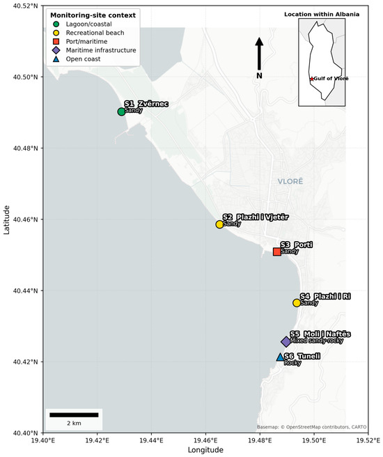
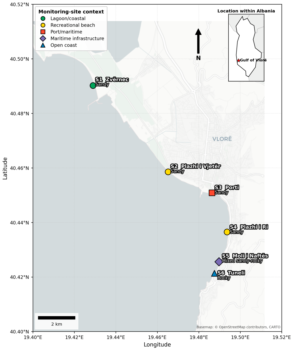
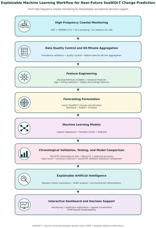
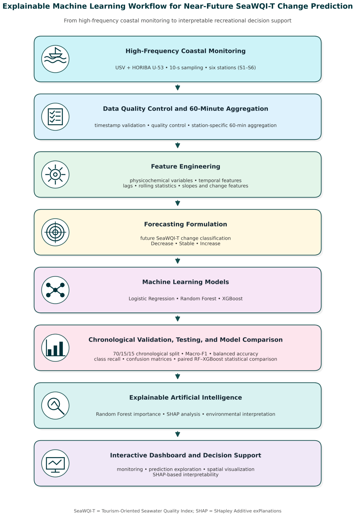
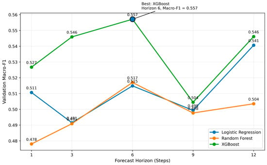
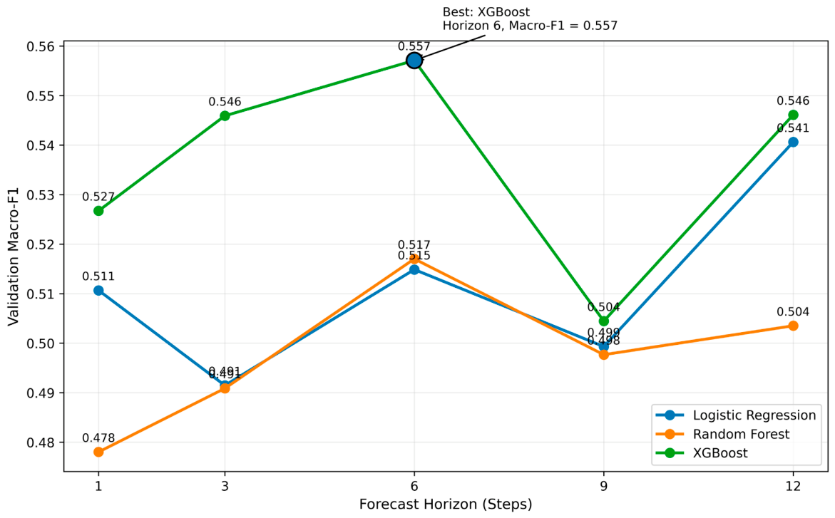
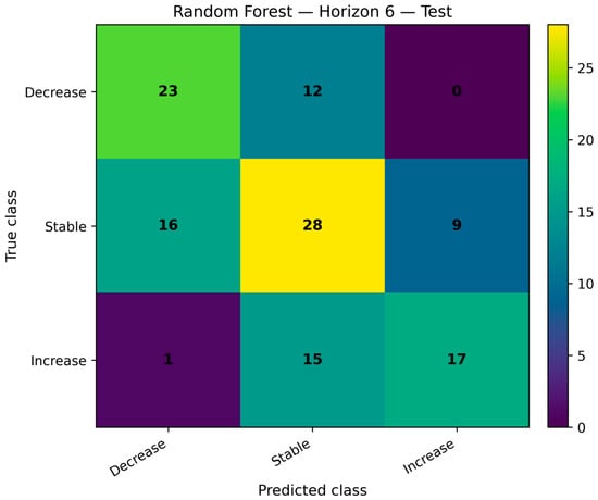
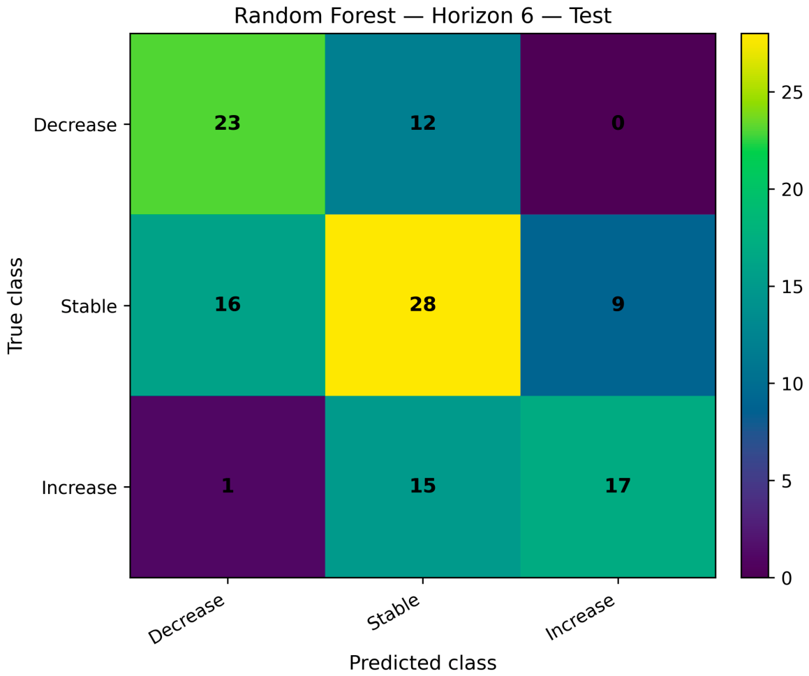
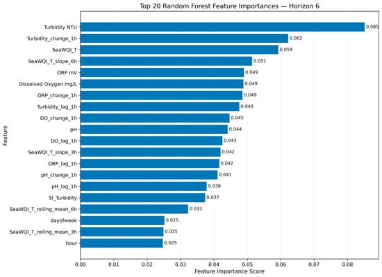
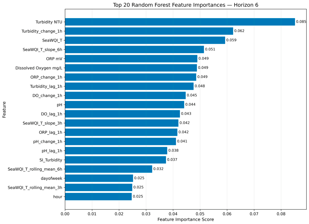
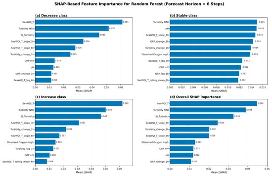
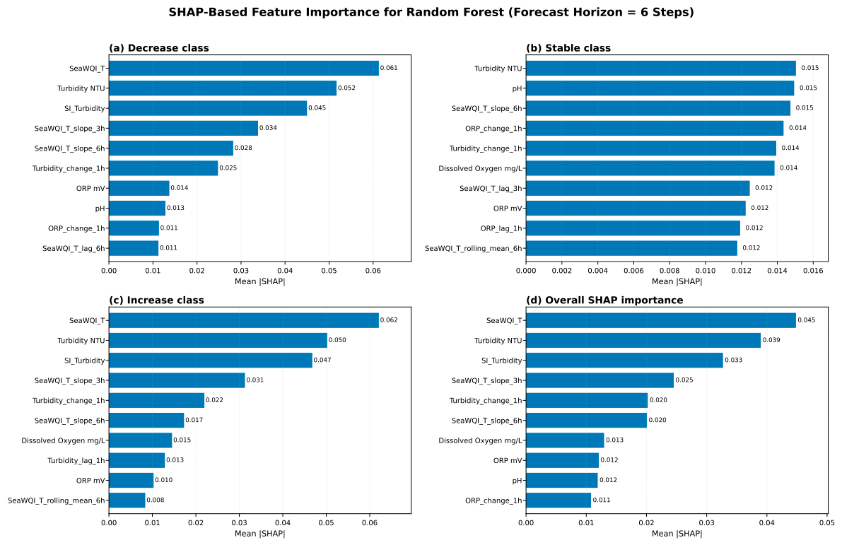
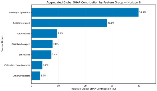
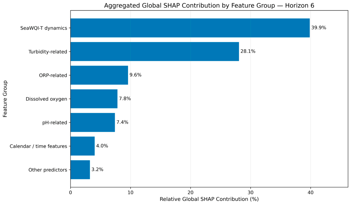
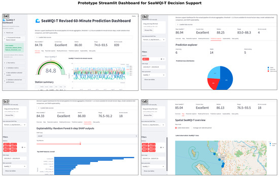
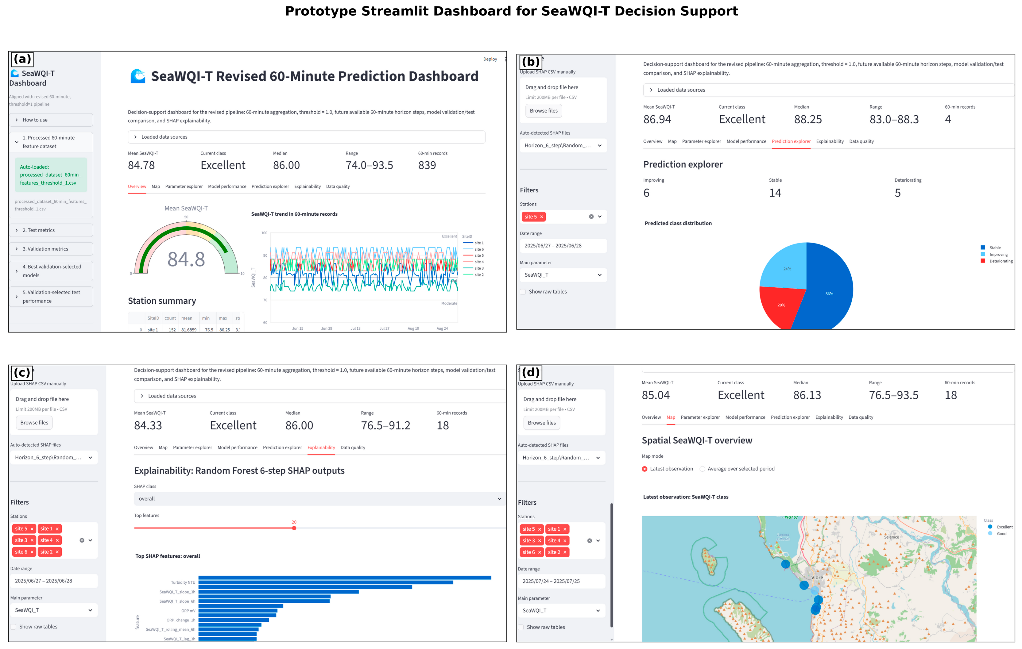

Disclaimer/Publisher’s Note: The statements, opinions and data contained in all publications are solely those of the individual author(s) and contributor(s) and not of MDPI and/or the editor(s). MDPI and/or the editor(s) disclaim responsibility for any injury to people or property resulting from any ideas, methods, instructions or products referred to in the content. |
© 2026 by the authors. Licensee MDPI, Basel, Switzerland. This article is an open access article distributed under the terms and conditions of the Creative Commons Attribution (CC BY) license.