Structural Changes in National Greenhouse Gas Intensity:Development of a Composite GHG Intensity Index for OECD Member Countries (2000–2020)

Abstract

This study assesses long-term structural changes in greenhouse gas (GHG) intensity across 38 OECD member countries over the period of 2000–2020 using a multidimensional Z-score standardization framework. GHG intensity was measured using three activity-based indicators—emissions per unit of land area, per capita emissions, and emissions per unit GDP—which were then aggregated into a Composite GHG Intensity Score (GHGIS) to facilitate cross-country comparison while accounting for differences in territorial scale, demographic structure, and economic output. The results reveal substantial heterogeneity in both the level and trajectory of composite GHG intensity across OECD member states. Countries such as Sweden (ΔScore = −0.84) and Denmark (ΔScore = −0.67) demonstrated a decrease in GHGIS, reflecting relative improvements in emission efficiency, while Korea (ΔScore = +0.92) and Türkiye (ΔScore = +1.15) recorded positive shifts in relative positioning over the study period. Several countries, including the United Kingdom, Germany, Japan, and Israel, exhibited divergent trends across land-, population-, and GDP-based measures, highlighting the multidimensional nature of national emission structures. These findings demonstrate that relative changes in GHG intensity vary across structural dimensions and cannot be adequately characterized by single-indicator measures alone. While the analysis does not identify causal drivers of observed patterns, the standardized composite framework provides a transparent and replicable tool for examining long-term comparative shifts in multidimensional emission intensity. By applying a consistent methodology across all OECD member countries over two decades, the study contributes to comparative assessments of structural GHG intensity dynamics.

1. Introduction

Global climate change has intensified due to rising greenhouse gas (GHG) concentrations driven by anthropogenic activities since industrialization [1,2,3]. According to the World Meteorological Organization, the global average temperature in 2020 was approximately 1.2 °C above the pre-industrial baseline [4]. The Intergovernmental Panel on Climate Change (IPCC) has emphasized that limiting warming to 1.5 °C requires rapid and sustained emission reductions; specifically, global GHG emissions must decline substantially from 2010 levels by 2030 to mitigate severe climate risks [5,6,7,8,9]. These findings have reinforced international commitments to carbon neutrality under frameworks such as the United Nations Framework Convention on Climate Change (UNFCCC) [10,11,12]. Carbon dioxide (CO₂), the primary component of anthropogenic GHG emissions, remains the primary driver of global warming and the resulting environmental instability [13,14].

However, evaluating national emission performance necessitates more than merely monitoring total emissions. Absolute emission levels are heavily influenced by economic scale, population size, and territorial extent, rendering direct comparisons across heterogeneous countries methodologically constrained [15,16,17,18]. Consequently, greenhouse gas intensity (GHGI)—defined as emissions per unit of economic output, population, or activity—has become a widely adopted indicator of emission efficiency [19,20]. Intensity-based measures facilitate structural comparisons by normalizing for differences in national scale and development stages [21,22].

Previous research has predominantly employed single-dimensional GHG intensity indicators, particularly emissions per unit of GDP, to assess environmental performance [23]. While informative, such measures may insufficiently capture structural heterogeneity related to demographic density and territorial scale. Some studies have incorporated additional denominators, such as land area and population, or constructed composite indices [24,25]. Nevertheless, comprehensive longitudinal benchmarking across the full set of OECD member states remains limited [26,27,28,29].

In this study, the term “structural” denotes multidimensional differences in emission intensity associated with territorial, demographic, and economic scaling factors, rather than formal structural decomposition analysis. Although analytically parsimonious, the framework is designed to enhance comparability and reduce aggregation bias by integrating these determinants into a unified standardized index. By doing so, it provides a multidimensional assessment of national emission efficiency and offers robust empirical evidence for identifying relative structural improvements across diverse national contexts. Compared to previous studies [24,25], which focused on single-dimensional measures or region-specific samples, this study applies a standardized multidimensional framework to the entire OECD over a 20-year period, establishing a consistent longitudinal benchmarking structure that has been limited in prior research.

2. Research Data and Methods

2.1. Research Scopes

The OECD is an international organization comprising 38 member countries worldwide (

Table 1. OECD member countries.

No.	Countries	Abbreviation	Year of OECD Accession	No.	Countries	Abbreviation	Year of OECD Accession
1	Australia	AUS	1971	20	Japan	JPN	1964
2	Austria	AUT	1961	21	Korea	KOR	1996
3	Belgium	BEL	1961	22	Latvia	LVA	2016
4	Canada	CAN	1961	23	Lithuania	LTU	2018
5	Chile	CHL	2010	24	Luxembourg	LUX	1961
6	Colombia	COL	2020	25	Mexico	MEX	1994
7	Costa Rica	CRI	2021	26	Netherlands	NLD	1961
8	Czechia	CZE	1961	27	New Zealand	NZL	1973
9	Denmark	DNK	1961	28	Norway	NOR	1961
10	Estonia	EST	2010	29	Poland	POL	1996
11	Finland	FIN	1969	30	Portugal	PRT	1961
12	France	FRA	1961	31	Slovak Republic	SVK	2000
13	Germany	DEU	1961	32	Slovenia	SVN	2010
14	Greece	GRC	1961	33	Spain	ESP	1961
15	Hungary	HUN	1996	34	Sweden	SWE	1961
16	Iceland	ISL	1961	35	Switzerland	CHE	1961
17	Ireland	IRL	1961	36	Türkiye	TUR	1961
18	Israel	ISR	2010	37	United Kingdom	GBR	1961
19	Italy	ITA	1962	38	United States	USA	1961

Source: http://www.oecd.org/ [30].

). Founded on core values such as market economies, pluralistic democracy, and respect for human rights, it functions as a premier intergovernmental body for policy research and cooperation, designed to promote sustainable economic development and enhance socio-economic well-being.

All member countries publish comprehensive and standardized datasets, including greenhouse gas (GHG) inventories, energy statistics, GDP, industrial value-added data, trade data, and environmental regulations (e.g., carbon taxes). The availability of such high-fidelity data facilitates the analysis of structural determinants driving GHG emissions, including advanced economic and industrial frameworks, the prevalence of energy-intensive sectors, and high levels of urbanization.

OECD member states were specifically selected for this study due to the accessibility of standardized, long-term statistical data, which ensures robust cross-country comparability and longitudinal consistency.

2.2. Research Data Source

2.2.1. OECD Member Countries Data Base Value (Total GHG Emissions)

For consistency, the data used in this study were collected from the official OECD website, focusing on total greenhouse gas emissions from OECD member countries over the past 20 years.

Table 2. GHG emissions by OECD member countries (2000–2020) (Unit: Thousand ton CO₂-eq).

Countries	2000	2010	2020	Remarks	Countries	2000	2010	2020	Remarks
AUS	501,588.99	547,172.76	536,739.72		JPN	1,373,303.42	1,300,046.75	1,144,932.50
AUT	80,619.36	84,693.29	73,910.84		KOR	502,730.45	656,119.74	656,222.88
BEL	148,877.33	133,644.30	107,272.65		LVA	10,167.78	11,857.88	10,483.14
CAN	719,463.71	701,867.55	658,788.39		LTU	19,493.65	20,741.77	20,165.73
CHL	71,498.72	86,969.65	105,551.92		LUX	9635.00	12,159.05	9029.90
COL	120,643.72	155,060.42	180,727.24	Data as of 2018	MEX	587,814.41	719,697.30	736,629.57	Data as of 2019
CRI	9945.75	12,895.96	14,477.30	Data as of 2017	NLD	219,454.92	214,236.64	164,367.79
CZE	151,139.21	140,167.57	113,072.05		NZL	74,850.47	77,328.02	77,330.66
DNK	72,662.45	65,857.45	44,483.80		NOR	54,074.16	54,925.06	49,214.64
EST	17,453.34	21,111.60	11,407.08		POL	393,992.73	407,236.96	371,312.43
FIN	70,136.61	75,555.95	47,756.28		PRT	82,420.02	69,529.86	58,029.35
FRA	548,714.51	511,152.92	398,297.03		SVK	48,986.21	45,766.63	37,187.89
DEU	1,040,191.83	932,379.13	730,922.69		SVN	18,769.38	19,797.93	15,974.78
GRC	126,659.45	119,159.95	75,464.49		ESP	383,276.36	354,652.28	272,244.36
HUN	75,378.31	66,533.79	62,965.32		SWE	68,349.11	64,375.65	46,214.03
ISL	4154.23	4906.35	4521.06		CHE	53,839.34	55,306.85	43,789.74
IRL	69,712.38	63,032.16	59,056.30		TUR	298,916.75	398,793.16	523,990.82
ISR	67,162.86	75,241.03	77,674.84		GBR	723,919.58	615,724.59	408,965.08
ITA	559,978.14	523,465.70	384,969.88		USA	7,369,162.97	7,058,197.91	6,025,973.61

Source: http://www.oecd.org/. Pollutant: Greenhouse Gases. Variable: Total emissions excluding LULUCF. Unit: Tones of CO₂ equivalent, Thousands.

presents the total greenhouse gas emissions of the 38 OECD member countries from 2000 to 2020.

If data for the year 2020 were not available, the most recently updated year was used instead. The corresponding countries are Colombia (2018), Croatia (2017), and Mexico (2019).

Although substituting the most recent available year ensures dataset completeness, this approach may introduce minor comparability bias due to short-term fluctuations in emission intensity. However, because the analysis focuses on long-term structural trends over a 20-year period and relies on standardized cross-sectional comparisons, the influence of a one- or two-year discrepancy is expected to be limited. Nevertheless, these data limitations should be acknowledged when interpreting country-level ΔScore magnitudes.

2.2.2. Data Variables for OECD Member Countries (Land, Population, GDP)

GHG emissions policy is not simply a technical measure to reduce emissions; rather, it involves adjustments across the entire social, economic, and ecological system [31]. Land area, population, and GDP represent core structural dimensions commonly associated with national emission patterns, reflecting territorial scale, demographic activity, and economic production capacity. These three factors directly influence emission levels, shape policy effectiveness, and provide a structural basis for evaluating emission reduction strategies.

Therefore, in this study, annual data on land area, population, and GDP for OECD member countries were collected for GHG intensity analysis (

Table 3. Variable Values [Land, Population, GDP] by OECD member countries (2000–2020).

Countries	Variable	2000	2010	2020	Countries	Variable	2000	2010	2020
AUS	Land	7,741,220	7,741,220	7,741,220	JPN	Land	377,800	377,950	377,974
	Population	19,028,802	22,031,750	25,655,289		Population	126,925,843	128,057,352	126,146,099
	GDP	410.13	1301.24	1435.44		GDP	4968.36	5759.07	5055.59
AUT	Land	83,879	83,879	83,879	KOR	Land	99,260	100,030	100,410
	Population	8,011,566	8,361,069	8,916,845		Population	47,008,111	49,554,112	51,836,239
	GDP	196.18	389.83	434.40		GDP	597.80	1192.83	1744.07
BEL	Land	30,528	30,528	30,528	LVA	Land	64,594	64,594	64,590
	Population	10,251,251	10,895,591	11,506,938		Population	2,367,549	2,097,553	1,900,448
	GDP	236.79	481.56	529.69		GDP	7.76	23.48	33.38
CAN	Land	15,640,500	15,640,500	15,640,500	LTU	Land	65,300	65,300	65,290
	Population	30,685,730	34,004,889	38,007,166		Population	3,499,534	3,097,282	2,794,885
	GDP	744.63	1617.35	1655.69		GDP	11.55	36.65	57.41
CHL	Land	756,096	756,096	756,700	LUX	Land	2590	2590	2590
	Population	15,343,326	17,063,927	19,458,310		Population	436,303	506,953	630,413
	GDP	78.24	217.11	253.88		GDP	21.23	56.21	73.70
COL	Land	1,141,750	1,141,750	1,140,619	MEX	Land	1,964,380	1,964,380	1,964,375
	Population	39,140,080	44,086,292	50,407,647		Population	98,785,275	113,748,671	127,792,286
	GDP	93.45	286.50	270.35		GDP	742.06	1105.42	1121.06
CRI	Land	51,100	51,100	51,100	NLD	Land	41,530	41,540	41,540
	Population	3,872,349	4,533,894	5,111,238		Population	15,925,505	16,615,390	17,441,500
	GDP	15.01	37.66	62.40		GDP	417.65	852.46	932.56
CZE	Land	78,870	78,870	78,871	NZL	Land	267,710	267,710	267,710
	Population	10,272,503	10,517,247	10,700,155		Population	3,857,700	4,350,700	5,090,200
	GDP	62.17	211.17	251.11		GDP	54.44	146.52	212.70
DNK	Land	42,920	42,920	42,920	NOR	Land	385,178	385,178	385,178
	Population	5,337,344	5,543,819	5,825,337		Population	4,490,973	4,889,253	5,379,472
	GDP	164.04	322.35	355.63		GDP	171.46	431.05	367.63
EST	Land	45,230	45,230	45,340	POL	Land	312,690	312,680	312,710
	Population	1,396,985	1,331,475	1,329,479		Population	38,258,478	38,516,689	38,354,173
	GDP	5.69	19.54	31.82		GDP	172.95	478.11	605.91
FIN	Land	338,150	338,420	338,460	PRT	Land	92,120	92,210	92,230
	Population	5,176,203	5,363,341	5,529,545		Population	10,289,898	10,573,100	10,384,846
	GDP	125.97	249.43	270.00		GDP	118.61	238.44	229.62
FRA	Land	549,087	549,087	549,087	SVK	Land	49,030	49,037	49,030
	Population	60,724,780	64,773,169	67,538,482		Population	5,400,679	5,431,024	5,458,827
	GDP	1360.96	2646.23	2647.93		GDP	20.70	91.11	107.73
DEU	Land	357,030	357,130	357,590	SVN	Land	20,270	20,270	20,480
	Population	82,211,501	81,776,936	83,160,877		Population	1,990,272	2,049,261	2,100,126
	GDP	1966.98	3468.15	3940.14		GDP	20.16	47.79	53.38
GRC	Land	131,960	131,960	131,960	ESP	Land	505,000	505,600	505,969
	Population	10,805,806	11,121,344	10,698,597		Population	40,554,387	46,562,483	47,355,685
	GDP	126.98	296.42	191.36		GDP	598.10	1427.99	1289.78
HUN	Land	93,030	93,030	93,030	SWE	Land	447,420	447,420	447,420
	Population	10,210,965	10,000,020	9,750,153		Population	8,872,112	9,378,131	10,353,444
	GDP	47.28	131.90	158.47		GDP	262.90	492.75	545.15
ISL	Land	103,000	103,000	103,000	CHE	Land	41,290	41,290	41,290
	Population	281,200	318,044	366,462		Population	7,184,250	7,824,910	8,638,169
	GDP	9.03	13.75	21.63		GDP	279.21	598.85	741.90
IRL	Land	70,280	70,280	70,280	TUR	Land	785,350	785,350	785,350
	Population	3,789,536	4,554,763	4,977,443		Population	64,268,751	73,142,162	83,384,688
	GDP	100.21	221.99	436.56		GDP	274.29	776.97	720.34
ISR	Land	22,070	22,070	22,070	GBR	Land	243,610	243,610	243,610
	Population	6,289,200	7,623,561	9,215,113		Population	58,886,065	62,759,456	67,081,234
	GDP	136.52	239.68	413.20		GDP	1665.46	2485.48	2696.78
ITA	Land	302,069	302,069	302,068	USA	Land	9,632,030	9,831,510	9,831,510
	Population	56,942,108	59,819,402	59,438,845		Population	282,162,411	309,327,143	331,511,512
	GDP	1149.66	2144.94	1907.48		GDP	10,250.95	15,048.97	21,354.11

Source: http://www.oecd.org/. 1. Land—Measure: Total area; Combined unit of measure: Square kilometres. 2. Population—Measure: Population; Time horizon: Historical; Combined unit of measure: Persons. 3. GDP—Frequency of observation: Annual; Measure: Gross domestic product; Combined unit of measure: S dollars, exchange rate converted, Billions, Current prices.

). In this study, land area refers strictly to the terrestrial surface of each country and excludes maritime zones and dependent island territories. The values correspond to the official land surface statistics reported by the OECD Data Explorer. This definition ensures consistency across countries and avoids distortions associated with the inclusion of maritime areas in national statistics.

All land area values used in this study were cross-checked for consistency and systematically applied across all calculations. Any corrections to land area data (e.g., for Norway and Sweden) were fully incorporated into the recalculation of land-based GHG intensity, Z-scores, and composite indices, ensuring internal consistency throughout the analysis.

2.3. Research Methods

This study applies a four-equation framework to evaluate cross-national GHG intensity dynamics across OECD member countries. The methodological procedure consists of three stages:

(1)

Calculation of baseline GHG intensity indicators;

(2)

Z-score standardization;

(3)

Construction of a composite index with temporal comparison.

2.3.1. Baseline GHG Intensity (GHGI)

Greenhouse gas intensity (GHGI) is defined as total greenhouse gas emissions divided by a structural variable:

$${GHGI}_{(i,k,t)}={\displaystyle \frac{{Emissions}_{(i,t)}}{{Variable Factor}_{(i,k,t)}}}$$

where i denotes country, k represents the structural factor (land area, population, or GDP), and t denotes year. Land area, population, and GDP represent territorial, demographic, and economic dimensions of national emission systems. It should be noted that land-based intensity does not represent production efficiency in the conventional economic sense. Rather, it reflects spatial emission pressure or territorial concentration of emissions. In this framework, land area is included as a complementary structural dimension to capture spatial heterogeneity alongside demographic and economic factors.

2.3.2. Z-Score Standardization

To ensure cross-country comparability, each GHGI variable was standardized using Z-score normalization:

$$Z_{(i,k,t)}={\displaystyle \frac{{GHGI}_{(i,k,t)}-{\mu }_{(k,t)}}{{\sigma }_{(k,t)}}}$$

where μ and σ represent the cross-sectional mean and standard deviation of GHGI for factor k in year t. Positive values indicate above-average intensity relative to the OECD mean, while negative values indicate below-average positioning. It should be emphasized that Z-score standardization does not eliminate or mechanically mitigate extreme values. Rather, it rescales observations relative to the cross-sectional mean and standard deviation within each year. As a result, the composite index reflects relative positioning across countries, and observations that are statistically distant from the mean may still exhibit large standardized values.

2.3.3. Composite GHG Intensity Score (GHGIS)

The composite score was calculated as the arithmetic mean of the three standardized indicators:

$${Score}_{(i,t)}={\displaystyle \frac{Z_{(i,land,t)}+Z_{(i,pop,t)}+Z_{(i,gdp,t)}}{3}}$$

Equal weighting was applied to maintain dimensional neutrality and to avoid imposing normative assumptions regarding the relative importance of territorial, demographic, and economic dimensions. Although land area exhibits limited temporal variation compared with population and GDP, it was retained as an equal component because it captures spatial emission pressure and territorial constraints that influence national emission structures. As a robustness check, principal component analysis (PCA) was conducted (Appendix A), and alternative weighting schemes based on PCA loadings produced largely consistent country rankings and ΔScore patterns, indicating that the results are not sensitive to the weighting structure.

Prior to constructing the composite index, pairwise correlation analysis was conducted among the three standardized indicators (Z_land, Z_pop, Z_gdp) to examine potential dimensional redundancy. The results indicated moderate but not excessive correlations, suggesting partial association without full collinearity. To further assess the latent structure, principal component analysis (PCA) was performed (Appendix A). The PCA results showed that although the first component captured a substantial share of variance, the remaining components retained non-negligible explanatory power, supporting the interpretation of the three indicators as related yet distinct structural dimensions rather than a single latent factor.

Because all indicators are standardized using the same cross-sectional OECD reference group within each year, their aggregation preserves internal consistency and cross-dimensional comparability.

2.3.4. Temporal Change

Temporal change was measured as

$${∆Score}_i={GHGIS}_{(i,2020)}-{GHGIS}_{(i,2000)}$$

whereas a positive value indicates an upward shift. A supplementary linear trend analysis (2000–2020) was conducted as a robustness check, yielding results consistent with ΔScore patterns.

3. Research Results

3.1. GHG Intensity Results and Comparative Analysis (2000–2020)

The analysis reveals that the direction and magnitude of changes in GHG intensity vary across the three indicators. Land-based intensity remained relatively low in territorially large countries such as Australia, Canada, and the United States, while countries with limited land area—including Belgium, the Netherlands, and Korea—exhibited comparatively higher land-based intensity values.

Population-based intensity generally declined in many OECD member countries over the study period, whereas a smaller number of countries experienced increases. GDP-based intensity showed broad reductions across much of the OECD, although several countries recorded weaker improvements or relative deterioration.

These cross-indicator differences highlight that national emission performance depends on multiple structural dimensions. The present analysis does not attempt to determine causal drivers of these variations; rather, it identifies comparative structural patterns observable across countries and over time.

Table 4. Year-specific cross-sectional standardized Composite GHG Intensity Scores (GHGIS) for OECD member countries in 2000 and 2020.

Countries	(a) GHG Intensity by Land (GHG Emissions/Land)				(b) GHG Intensity by Population (GHG Emissions/Population)				(c) GHG Intensity by GDP (GHG Emissions/GDP)
	2000	2010	2020	Rank Change	2000	2010	2020	Rank Change	2000	2010	2020	Rank Change
AUS	6.48	7.07	6.93	-	2.64	2.48	2.09	-	122,300.20	42,050.11	37,391.90	▲ 1
AUT	96.11	100.97	88.12	▲ 3	1.01	1.01	0.83	▲ 3	41,094.25	21,725.82	17,014.56	▲ 6
BEL	487.67	437.78	349.55	▼ 1	1.45	1.23	0.93	▼ 3	62,872.50	27,752.57	20,251.80	▲ 2
CAN	4.60	4.49	4.21	▼ 1	2.34	2.06	1.73	-	96,620.12	43,396.27	39,789.46	▲ 8
CHL	9.46	11.50	13.95	▲ 2	0.47	0.51	0.54	▲ 1	91,388.82	40,058.72	41,575.48	▲ 11
COL	10.57	13.58	20.43	▲ 4	0.31	0.35	0.46	▲ 2	129,104.65	54,122.59	66,849.77	▼ 27
CRI	19.46	25.24	27.61	▲ 2	0.26	0.28	0.28	-	66,244.09	34,244.36	23,202.91	▼ 17
CZE	191.63	177.72	143.36	-	1.47	1.33	1.06	▼ 1	243,102.65	66,377.07	45,028.95	▼ 1
DNK	169.30	153.44	103.64	▼ 2	1.36	1.19	0.76	▼ 9	44,294.78	20,430.70	12,508.41	▼ 1
EST	38.59	46.68	25.16	▼ 5	1.25	1.59	0.86	▼ 3	306,693.51	108,065.15	35,847.91	▼ 10
FIN	20.74	22.33	14.11	▼ 3	1.35	1.41	0.86	▼ 4	55,678.20	30,291.49	17,687.49	▼ 1
FRA	99.93	93.09	72.54	▼ 4	0.90	0.79	0.59	▼ 2	40,318.22	19,316.27	15,041.85	▲ 5
DEU	291.35	261.08	204.40	▲ 1	1.27	1.14	0.88	▼ 2	52,882.67	26,884.01	18,550.67	▲ 1
GRC	95.98	90.30	57.19	▼ 5	1.17	1.07	0.71	▼ 6	99,750.55	40,200.02	39,435.26	▲ 5
HUN	81.03	71.52	67.68	▲ 2	0.74	0.67	0.65	▲ 5	159,443.21	50,443.08	39,733.65	-
ISL	4.03	4.76	4.39	▲ 1	1.48	1.54	1.23	-	46,026.85	35,679.53	20,901.85	▲ 9
IRL	99.19	89.69	84.03	▲ 1	1.84	1.38	1.19	▼ 2	69,567.95	28,394.70	13,527.79	▼ 11
ISR	304.32	340.92	351.95	▲ 3	1.07	0.99	0.84	▲ 2	49,197.60	31,392.42	18,798.54	▲ 4
ITA	185.38	173.29	127.44	-	0.98	0.88	0.65	▼ 2	48,708.09	24,404.72	20,182.11	▲ 6
JPN	363.50	343.97	302.91	▼ 1	1.08	1.02	0.91	▲ 4	27,640.99	22,573.89	22,646.88	▲ 18
KOR	506.48	655.92	653.54	▲ 1	1.07	1.32	1.27	▲ 13	84,096.53	55,005.30	37,625.94	▲ 8
LVA	15.74	18.36	16.23	-	0.43	0.57	0.55	▲ 4	131,002.66	50,510.64	31,405.52	▼ 6
LTU	29.85	31.76	30.89	▲ 2	0.56	0.67	0.72	▲ 11	168,763.12	56,597.63	35,124.57	▼ 7
LUX	372.01	469.46	348.64	▼ 1	2.21	2.40	1.43	▼ 1	45,383.50	21,629.94	12,252.34	▼ 3
MEX	29.92	36.64	28.12	▼ 1	0.60	0.63	0.43	▼ 5	79,213.73	65,105.98	65,708.03	▼ 20
NLD	528.43	515.74	395.69	▼ 1	1.38	1.29	0.94	▼ 1	52,545.26	25,131.43	17,625.42	-
NZL	27.96	28.88	28.89	▲ 2	1.94	1.78	1.52	▲ 1	137,480.85	52,777.57	36,357.32	▼ 3
NOR	14.04	14.26	7.88	▼ 2	1.20	1.12	0.91	▲ 3	31,538.14	12,742.09	13,386.88	▲ 4
POL	126.00	130.24	118.74	▲ 2	1.03	1.06	0.97	▲ 11	227,802.66	85,176.12	61,281.35	▲ 2
PRT	89.47	75.40	62.92	▼ 1	0.80	0.66	0.56	▼ 3	69,491.07	29,159.84	25,272.04	▲ 3
SVK	99.91	93.33	75.85	▼ 2	0.91	0.84	0.68	▲ 2	236,643.85	50,231.09	34,518.70	▼ 10
SVN	92.60	97.67	78.00	▲ 3	0.94	0.97	0.76	▲ 4	93,098.54	41,424.23	29,923.86	▼ 1
ESP	75.90	70.14	53.81	▼ 1	0.95	0.76	0.57	▼ 6	64,082.01	24,835.78	21,107.75	▲ 3
SWE	15.28	14.39	8.74	▼ 2	0.77	0.69	0.45	▼ 7	25,997.75	13,064.48	8477.34	▲ 3
CHE	130.39	133.95	106.05	-	0.75	0.71	0.51	▼ 4	19,282.81	9235.49	5902.36	▲ 3
TUR	38.06	50.78	66.72	▲ 5	0.47	0.55	0.63	▲ 8	108,976.44	51,326.90	72,742.31	▲ 10
GBR	297.16	252.75	167.88	▼ 1	1.23	0.98	0.61	▼ 13	43,466.72	24,772.84	15,164.95	▲ 4
USA	76.51	71.79	61.29	-	2.61	2.28	1.82	-	71,887.60	46,901.53	28,219.27	▲ 2

Note: GHGIS values are cross-sectional Z-score-standardized composite indicators for each respective year. ΔScore represents the standardized change between 2000 and 2020 (2020–2000). Negative ΔScore values indicate relative improvement in emission efficiency. Rank Change indicates the shift in each country’s relative ranking position between 2000 and 2020 within the OECD sample. “▲” indicates an increase in ranking position, while “▼” indicates a decrease in ranking position.

reports the standardized composite GHG intensity scores for 2000 and 2020, along with the absolute change (ΔScore) between the two years. The reported values are not period averages but year-specific cross-sectional standardized scores.

Large upward or downward rank changes shown in Table 4 primarily reflect asymmetric movements across the three structural intensity dimensions rather than uniform change in a single indicator. In several cases, substantial improvements in GDP-based intensity were partially offset by weaker progress or deterioration in land- or population-based measures, leading to complex net rank shifts. Moreover, because the rankings are calculated relative to the OECD cross-sectional benchmark in each year, rank variation may also result from changes in the performance of other member countries. Therefore, large rank shifts should be interpreted as reflecting both domestic structural adjustments and evolving comparative positioning within the OECD group.

Rank change thus serves as an ordinal indicator of relative movement within the OECD comparison framework, complementing the magnitude-based ΔScore metric.

Revisions to land area values result in only minor numerical adjustments and do not materially affect country rankings, rank changes, or the overall analytical conclusions.

It should be noted that the reported rank changes represent relative positional shifts among OECD countries between 2000 and 2020, rather than the absolute change in indicator values. Therefore, a country may experience a decline in ranking even when its emission intensity decreases, if other countries achieve larger reductions over the same period.

3.2. Z-Score Standardization

To enable cross-country comparability, all GHG intensity indicators were standardized using Z-score normalization. This transformation rescales each indicator to a mean of zero and a standard deviation of one within each year, allowing relative comparison independent of unit scale. Positive Z-scores indicate above-average intensity relative to the OECD mean, whereas negative values indicate relatively lower intensity.

The standardized results confirm substantial heterogeneity across countries (

Table 5. Component-wise cross-sectional Z-score-standardized GHG intensity indicators for OECD member countries in 2000 and 2020, with average composite values and fluctuation measures (Standard: Z-Score < 0 (High efficiency), Z-Score > 0 (Low efficiency)).

Countries	2000			2020			Avg		Fluctuation Value
	Z_LAN	Z_POP	Z_GDP	Z_LAN	Z_POP	Z_GDP	2000	2020
AUS	−0.86	2.49	0.43	−0.77	2.97	0.76	0.69	0.99	0.30
AUT	−0.26	−0.26	−0.77	−0.19	−0.12	−0.53	−0.43	−0.28	0.15
BEL	2.34	0.48	−0.45	1.66	0.13	−0.32	0.79	0.49	−0.31
CAN	−0.87	1.99	0.05	−0.78	2.09	0.91	0.39	0.74	0.35
CHL	−0.84	−1.18	−0.03	−0.72	−0.83	1.02	−0.68	−0.17	0.51
COL	−0.83	−1.45	0.53	−0.67	−1.03	−1.55	−0.58	−1.08	−0.50
CRI	−0.77	−1.53	−0.40	−0.62	−1.47	−1.59	−0.90	−1.22	−0.32
CZE	0.37	0.52	2.22	0.20	0.45	1.24	1.04	0.63	−0.41
DNK	0.23	0.33	−0.73	−0.08	−0.29	−0.81	−0.06	−0.39	−0.34
EST	−0.64	0.14	3.16	−0.64	−0.05	0.66	0.89	−0.01	−0.89
FIN	−0.76	0.31	−0.56	−0.71	−0.05	−0.48	−0.34	−0.41	−0.08
FRA	−0.24	−0.45	−0.78	−0.30	−0.71	−0.65	−0.49	−0.55	−0.06
DEU	1.04	0.18	−0.60	0.63	0.00	−0.43	0.21	0.07	−0.14
GRC	−0.26	0.01	0.10	−0.41	−0.41	0.89	−0.05	0.02	0.07
HUN	−0.36	−0.72	0.98	−0.34	−0.56	0.91	−0.03	0.00	0.04
ISL	−0.87	0.53	−0.70	−0.78	0.86	−0.28	−0.35	−0.07	0.28
IRL	−0.24	1.14	−0.35	−0.22	0.76	−0.75	0.18	−0.07	−0.25
ISR	1.12	−0.16	−0.65	1.67	−0.09	−0.41	0.10	0.39	0.28
ITA	0.33	−0.31	−0.66	0.09	−0.56	−0.33	−0.21	−0.27	−0.05
JPN	1.52	−0.14	−0.97	1.33	0.08	−0.17	0.13	0.41	0.28
KOR	2.47	−0.16	−0.14	3.80	0.96	0.77	0.72	1.85	1.12
LVA	−0.80	−1.24	0.56	−0.70	−0.81	0.38	−0.49	−0.37	0.12
LTU	−0.70	−1.02	1.12	−0.60	−0.39	0.62	−0.20	−0.12	0.08
LUX	1.57	1.77	−0.71	1.65	1.35	−0.83	0.88	0.73	−0.15
MEX	−0.70	−0.96	−0.21	−0.62	−1.10	−1.57	−0.62	−1.10	−0.47
NLD	2.61	0.36	−0.60	1.98	0.15	−0.49	0.79	0.55	−0.24
NZL	−0.71	1.31	0.66	−0.61	1.58	0.69	0.42	0.55	0.14
NOR	−0.81	0.06	−0.91	−0.76	0.08	−0.76	−0.55	−0.48	0.08
POL	−0.06	−0.23	1.99	0.02	0.22	2.27	0.57	0.84	0.27
PRT	−0.31	−0.62	−0.35	−0.37	−0.78	−0.01	−0.43	−0.39	0.04
SVK	−0.24	−0.43	2.12	−0.28	−0.49	0.58	0.49	−0.06	−0.55
SVN	−0.28	−0.38	0.00	−0.26	−0.29	0.29	−0.22	−0.09	0.13
ESP	−0.40	−0.36	−0.43	−0.43	−0.76	−0.27	−0.40	−0.49	−0.09
SWE	−0.80	−0.67	−1.00	−0.75	−1.05	−1.07	−0.82	−0.96	−0.14
CHE	−0.03	−0.70	−1.10	−0.06	−0.90	−1.23	−0.61	−0.73	−0.12
TUR	−0.65	−1.18	0.23	−0.34	−0.61	2.99	−0.53	0.68	1.21
GBR	1.08	0.11	−0.74	0.37	−0.66	−0.64	0.15	−0.31	0.12
USA	−0.39	2.44	−0.32	−0.38	2.31	0.18	0.58	0.70	−0.46

Note: Z_LAN, Z_POP, and Z_GDP represent cross-sectional Z-score-standardized GHG intensity indicators based on land area, population, and GDP, respectively, for each given year. “Avg” represents the arithmetic mean of the three standardized component scores for the respective year. “Fluctuation Value” indicates the change in the average composite value between 2000 and 2020 (2020–2000). Negative Z-score values indicate relatively higher emission efficiency compared to the OECD mean for that year.

). Several Western European countries maintained consistently negative average Z-scores over time, while a smaller group exhibited persistent positive values. In many cases, movements in Z_LAN, Z_POP, and Z_GDP diverged, underscoring the multidimensional nature of national emission structures.

Rather than interpreting these differences as policy outcomes, the standardized results should be understood as descriptive indicators of relative structural positioning within the OECD group.

3.3. Composite Score & ΔScore

Among the 38 countries analyzed, Estonia and the Slovak Republic recorded the largest negative ΔScore values, indicating substantial relative improvement in composite GHG intensity between 2000 and 2020. Conversely, Türkiye and Korea recorded the largest positive ΔScore values, indicating relative deterioration over the same period.

Countries with moderate ΔScore values exhibited comparatively stable trajectories. In several cases, improvements in one structural dimension were offset by weaker performance in others, resulting in limited net change in the composite index.

The ΔScore metric should be interpreted as a measure of relative structural change within the OECD group rather than as a direct evaluation of policy effectiveness or economic performance. To strengthen the analytical rigor of the results, ordinary least squares (OLS) trend regressions were estimated for each country over the 2000–2020 period. The detailed regression results are reported in Appendix B.

For the majority of countries exhibiting clear upward or downward ΔScore patterns, the estimated trend coefficients were statistically significant (p < 0.05). These findings suggest that the observed composite intensity shifts reflect statistically meaningful long-term trends rather than purely descriptive fluctuations.

For presentation purposes, ΔScore values were multiplied by 100 to improve numerical readability. This transformation does not imply percentage change, as Z-scores are unitless standardized measures expressed in standard deviation units.

3.3.1. Cluster-Based Analysis of Structural Characteristics Using ΔScore

Countries were grouped based on similarities in ΔScore magnitude and Z-score trajectories. These clusters represent descriptive typologies rather than normative classifications.

• Group A: Increasing Composite Intensity
• (Korea, Türkiye, Poland, Czechia, Netherlands)

These countries exhibited higher average composite Z-scores in 2020 compared to 2000. The observed pattern suggests relative intensification across one or more structural dimensions during the study period.

• Group B: Low and Stable Intensity
• (Sweden, Switzerland, Denmark, Norway, France)

This group maintained consistently negative Z-scores across most indicators, indicating stable relative positioning within the lower-intensity range of OECD member countries.

• Group C: Mixed Structural Profiles
• (United Kingdom, Germany, Japan, Israel, New Zealand)

Countries in this category showed divergent movements across land-, population-, and GDP-based indicators, illustrating heterogeneous structural dynamics.

• Group D: Improving Composite Intensity
• (Ireland, Slovak Republic, Latvia, Lithuania)

These countries recorded decreasing average composite Z-scores between 2000 and 2020, indicating relative improvement in multidimensional intensity measures.

• Group E: Spatial–Economic Structural Profiles
• (Canada, Australia, Colombia, Chile)

These countries exhibited Z-score patterns influenced by combinations of territorial scale, population distribution, and economic structure. The results highlight how spatial characteristics interact with intensity metrics in cross-national comparisons.

3.3.2. Rank-Based Tier Classification

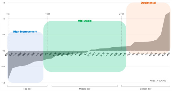
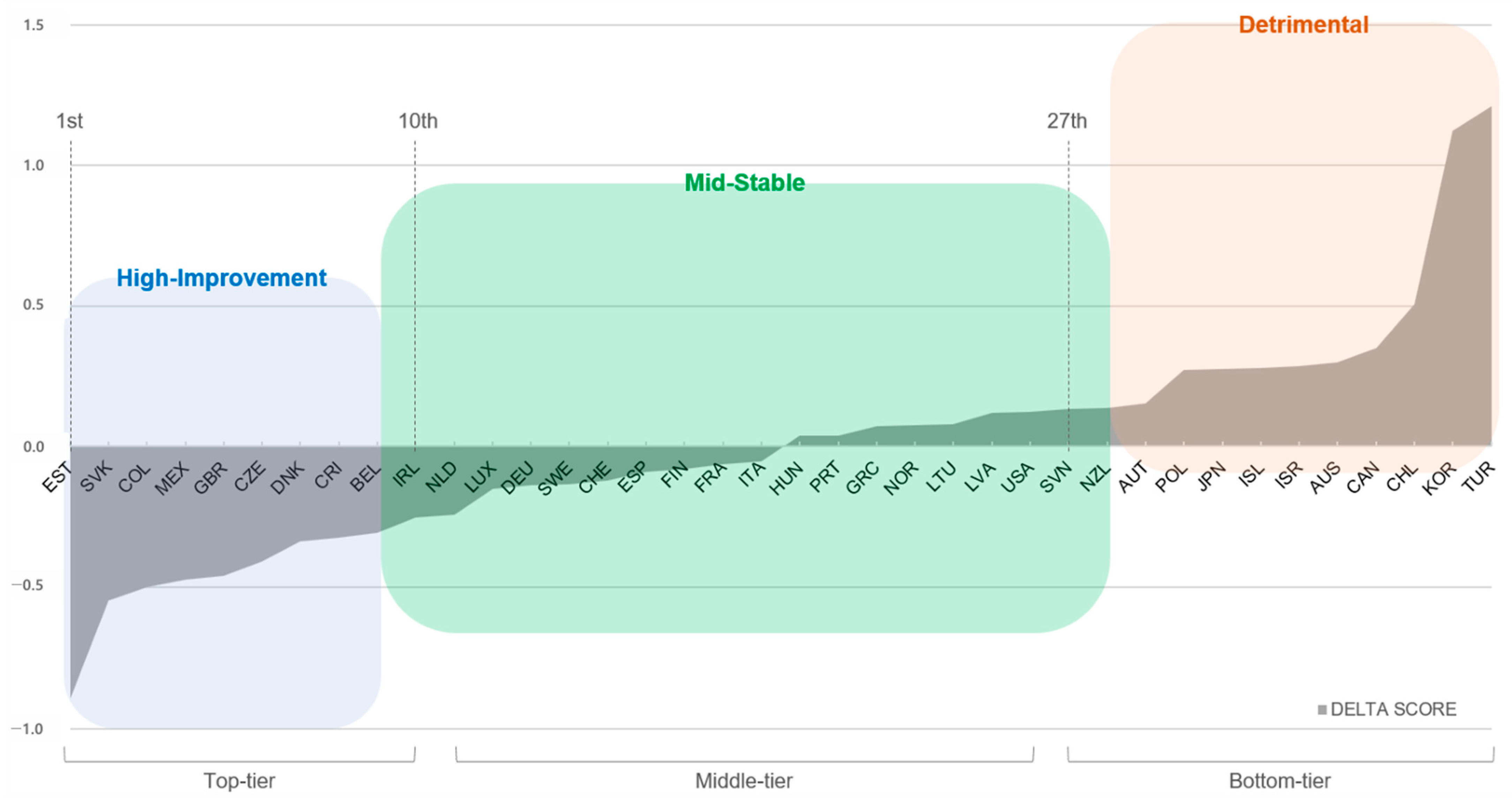
Countries are ordered from lowest to highest ΔScore. The vertical dashed lines indicate rank-based cutoffs (1st, 10th, and 27th positions) used to classify countries into High-Improvement, Mid-Stable, and Detrimental groups. This figure does not represent quartiles, medians, or other distributional summary statistics; rather, it illustrates ordinal ranking based on ΔScore values.

As shown in Figure 1, the ranked distribution of ΔScore values across OECD member countries exhibits substantial cross-national heterogeneity. The range of ΔScore extends from approximately –0.9 to over +1.1, reflecting wide variation in long-term structural intensity change. A relatively small group of countries exhibits strongly negative ΔScore values (High-Improvement tier), while the majority cluster within a narrower band around zero (Mid-Stable tier). The right tail of the distribution shows a smaller subset of countries with markedly positive ΔScore values, reflecting relative deterioration in composite standardized intensity.

The distribution is moderately asymmetric, with a steeper increase in ΔScore values in the upper tail compared to the lower tail. This pattern suggests that extreme upward shifts in relative intensity positioning are concentrated among a limited number of countries, whereas improvements are more gradually distributed. These differences reinforce the importance of examining relative positioning rather than relying solely on aggregate trends.

The figure is intended as a descriptive visualization of relative positioning rather than an inferential statistical representation. The tier boundaries reflect ordinal ranking positions rather than statistical thresholds.

Countries were additionally grouped into three tiers based on the magnitude and direction of ΔScore values between 2000 and 2020. This tier classification serves as a comparative benchmarking device within the OECD sample and does not imply normative evaluation of national policy effectiveness.

(a)

Top-tier (Rank 1–9)

Countries in this tier (Rank 1–9) recorded the largest negative ΔScore values during the study period, indicating relatively greater reductions in composite GHG intensity compared to other OECD members. These results reflect downward movements in one or more standardized intensity dimensions between 2000 and 2020. While the underlying drivers of these changes are not examined in this study, the observed pattern indicates measurable shifts in relative structural emission positioning within the OECD group.

(b)

Middle-tier (Rank 10–26)

This group exhibits ΔScore values close to zero, ranging from approximately –0.25 to +0.12, indicating limited net change in composite GHG intensity over the 20-year period. In many cases, reductions in one intensity dimension were partially offset by increases or weaker performance in others, resulting in overall stability in relative ranking. The stability observed in this tier reflects heterogeneous movements across land-, population-, and GDP-based indicators rather than uniform directional change.

(c)

Bottom-tier (Rank 27–38)

Countries in this tier recorded positive ΔScore values, indicating relative increases in composite GHG intensity between 2000 and 2020. These results correspond to upward shifts in one or more standardized intensity measures within the OECD comparison framework.

As with the other tiers, the classification reflects observed changes in relative structural positioning and should not be interpreted as a direct assessment of national mitigation policy design or economic strategy. In addition, the classification is based on national-level aggregate data and does not capture subnational heterogeneity, which may be substantial in geographically large or federally structured countries.

3.4. Comprehensive Results and Further Interpretation

3.4.1. Extended Discussion

The Z-score-based standardization applied in this study enables a structured comparison of relative GHG intensity across OECD member countries by normalizing emissions with respect to land area, population, and GDP. This approach facilitates cross-national comparability by reducing scale-related distortions and highlighting differences in structural positioning within the OECD group.

Changes in average Z-scores between 2000 and 2020 provide a descriptive measure of relative shifts in multidimensional emission intensity. Several countries, including Korea, Türkiye, and Poland, recorded higher average composite Z-scores in 2020 compared to 2000, indicating upward movement in relative intensity positioning within the OECD sample. In contrast, countries such as Sweden, Switzerland, Denmark, and France maintained consistently negative or declining average Z-scores over the same period, reflecting relatively stable low-intensity positioning in comparative terms.

These country-level patterns can be partially interpreted in light of differences in energy transition pathways and climate policy frameworks during the study period. For instance, Sweden’s persistently low composite intensity is consistent with its long-standing reliance on hydropower and nuclear energy, alongside early adoption of carbon pricing mechanisms. Korea and Türkiye, which recorded upward movements in composite intensity, experienced sustained industrial expansion and continued dependence on fossil fuel-based power generation, despite gradual renewable energy deployment. Such contrasts suggest that structural emission intensity trajectories are closely associated with national energy mix composition, industrial structure, and the timing and stringency of mitigation policies.

Importantly, the magnitude and direction of change differ across the three standardized indicators—Z_LAN, Z_POP, and Z_GDP—underscoring the multidimensional nature of national emission structures. In some countries, improvements in population- or GDP-based intensity measures coincided with persistently higher land-based intensity values. In others, relatively low land-based intensity coexisted with higher population- or GDP-based values. These cross-indicator divergences illustrate how territorial scale, demographic distribution, and economic activity interact differently across national contexts.

The findings therefore suggest that reliance on a single intensity indicator may obscure structural heterogeneity across countries. The multidimensional framework presented here provides a standardized benchmarking tool for examining relative emission intensity patterns without presuming causal explanations. While the present study does not assess policy effectiveness or determine the underlying drivers of observed changes, it offers an empirically consistent basis for comparative structural assessment within the OECD context.

3.4.2. Country-Level Interpretation and Descriptive Grouping

The following section categorizes countries based on similarities observed in their Z-score trajectories between 2000 and 2020. The grouping is intended as a descriptive typology derived from standardized intensity patterns and does not imply causal interpretation or normative evaluation (

Table 6. Structural Group Classification of OECD Member Countries Based on Composite Z-Score Trajectories (2000–2020).

Group	Representative Countries	Z-Score Characteristics (2000–2020)	Descriptive Structural Interpretation
A. Relative Increase Group	KOR, TUR, POL, CZE, NLD	Higher average composite Z-scores in 2020 compared to 2000; upward movement in land- and/or GDP-based intensity	Indicates relative upward shifts in composite intensity positioning within the OECD comparison framework
B. Low and Stable Group	SWE, CHE, DNK, NOR, FRA	Consistently negative Z-scores across most indicators; limited fluctuation over time	Reflects stable positioning within the lower-intensity range of OECD countries during the study period
C. Mixed-Pattern Group	GBR, DEU, JPN, ISR, NZL	Divergent movements across Z_LAN, Z_POP, and Z_GDP	Illustrates multidimensional heterogeneity, where improvement in one indicator coincides with stability or increase in another
D. Relative Improvement Group	IRL, SVK, LVA, LTU	Declining average composite Z-scores between 2000 and 2020	Indicates downward movement in relative intensity ranking within the OECD sample
E. Spatial–Structural Profile Group	CAN, AUS, COL, CHL	Distinct combinations of low land-based intensity and comparatively higher population- or GDP-based values	Highlights how territorial scale and demographic distribution interact with standardized intensity measures in cross-country comparison

).

The group classification is based solely on observed standardized intensity trajectories and is intended to facilitate comparative interpretation. It should not be interpreted as a direct assessment of national policy effectiveness or economic strategy.

4. Discussion

The foregoing analysis demonstrates that changes in emission efficiency among OECD member countries over the past two decades are not merely a function of aggregate emission reductions but are shaped by the interaction of economic structure, demographic dynamics, industrial composition, and policy orientation.

The empirical results show that several countries achieved improvements in composite intensity despite stable or moderately increasing total emissions, suggesting structural decoupling between economic growth and emission pressure. Conversely, some countries exhibited limited improvement or deterioration in intensity even when absolute emissions declined, indicating persistent structural inefficiencies.

As shown in Table 5, several countries exhibit divergent trajectories across component indicators, highlighting that composite Z-score changes may mask opposing trends in land-, population-, and GDP-based intensity dimensions.

The heterogeneity observed in ΔScore values highlights that emission performance cannot be adequately interpreted using single-dimension indicators such as GDP intensity alone. In particular, spatial emission pressure and demographic concentration appear to influence overall efficiency trajectories in ways that purely economic measures may overlook.

These findings imply that carbon mitigation strategies must account for country-specific structural characteristics rather than relying solely on uniform reduction targets. Policy effectiveness may depend on identifying dominant structural drivers of emissions within each national context, including land-use patterns, population density, and economic specialization.

Accordingly, future policy design should prioritize:

-

Identification of country-specific structural constraints;

-

Integrated assessment of economic, demographic, and spatial emission drivers;

-

Continuous monitoring using multidimensional intensity indicators to evaluate long-term structural progress.

To enhance practical relevance, policy recommendations should also incorporate concrete transitional pathways. For instance, targeted mitigation strategies may include sector-specific approaches such as decarbonizing power generation, enhancing industrial energy efficiency, promoting low-carbon transport systems, and implementing carbon pricing mechanisms. Linking the multidimensional structural assessment to these practical measures can improve the real-world applicability of the findings and support evidence-based policy formulation.

Beyond the OECD comparative perspective, the findings of this study should also be interpreted within the broader framework of international climate governance. Since the adoption of the United Nations Framework Convention on Climate Change (UNFCCC) in 1992, global mitigation efforts have evolved through the Kyoto Protocol and the Paris Agreement. These agreements emphasize nationally determined contributions (NDCs), transparency mechanisms, and long-term decarbonization pathways under differentiated national circumstances.

Within this framework, cross-national comparisons of structural emission intensity provide a complementary analytical perspective to absolute emission accounting. The multidimensional composite index developed in this study captures territorial, demographic, and economic dimensions simultaneously, aligning with the differentiated responsibility principle embedded in international climate governance.

Furthermore, assessment reports by the Intergovernmental Panel on Climate Change stress that deep decarbonization requires structural transformation in energy systems, land use, and industrial production. The heterogeneous ΔScore trajectories identified across OECD member countries illustrate varying structural transition pathways, reinforcing the need for multidimensional benchmarking tools when evaluating mitigation progress. While this study does not empirically test causal drivers of the observed variation, the cross-national heterogeneity in ΔScore trajectories is consistent with structural differences in industrial composition, demographic trends, and energy systems documented in prior comparative research. The present analysis adopts a descriptive benchmarking approach rather than a causal modeling framework. Future research could extend this work by applying econometric decomposition techniques or structural regression models to more rigorously identify the determinants of multidimensional emission intensity change.

While this study does not assess compliance with specific treaty obligations, it provides an empirically consistent comparative framework that may inform discussions on burden-sharing, structural transition, and long-term net-zero strategies within evolving international climate regimes.

While the proposed framework improves cross-national comparability, several limitations should be acknowledged. The use of equal weighting may not fully reflect the relative importance of individual intensity components, and alternative weighting schemes could yield different rankings. In addition, although the ΔScore captures long-term change, more sophisticated time-series approaches may further refine the assessment of structural dynamics.

In addition, this study does not explicitly incorporate LULUCF adjustments beyond their treatment in national inventory data, which may affect cross-country comparability given differences in land-use accounting practices. Furthermore, this study utilized current-price GDP due to data availability, which may not account for inflation effects; future studies should employ constant-price GDP for more refined longitudinal comparisons.

Finally, the analysis is conducted at the national level and does not capture subnational heterogeneity. In geographically large OECD member countries, emission patterns and mitigation policies may vary substantially across regions or states. Therefore, the classifications and rankings presented in this study should be interpreted as aggregate structural representations rather than reflections of uniform internal policy conditions. Future research could extend this framework to subnational datasets to better account for within-country variation.

5. Conclusions

This study examined long-term changes in greenhouse gas (GHG) intensity across OECD member countries between 2000 and 2020 by standardizing three activity-based indicators—land area, population, and GDP—using a Z-score framework and constructing a composite GHG intensity score (GHGIS). By focusing on relative standardized positioning rather than absolute emission levels, the analysis identified substantial heterogeneity in multidimensional intensity trajectories across countries.

The results demonstrate that changes in composite GHG intensity vary considerably in both magnitude and direction across the OECD sample. In several cases, improvements in one standardized dimension were accompanied by stability or relative increases in another, underscoring the multidimensional character of national emission structures. These findings indicate that reliance on a single intensity indicator may obscure structural differences that become visible when territorial, demographic, and economic factors are evaluated simultaneously.

The Z-score-based framework enhances cross-national comparability by minimizing scale effects and providing a consistent basis for assessing relative structural positioning within a common reference group. Rather than evaluating policy effectiveness or identifying causal drivers, the study offers a standardized descriptive tool for examining long-term shifts in emission intensity patterns. The Composite GHG Intensity Score (GHGIS) and its change over time (ΔScore) therefore contribute a replicable methodological approach for comparative structural assessment.

Several limitations should be acknowledged. First, the analysis relies on officially reported OECD GHG statistics, which may involve differences in reporting methodologies across countries. Second, the framework incorporates only three activity-based intensity dimensions and does not account for additional structural, sectoral, or technological variables that may influence emissions. Third, equal weighting was applied in constructing the composite score; alternative weighting schemes could produce different relative rankings.

Future research may extend this framework by incorporating additional structural indicators, applying alternative weighting or decomposition techniques, or examining non-OECD contexts to evaluate the robustness and broader applicability of the multidimensional standardization approach. Such extensions would further refine comparative analyses of long-term GHG intensity dynamics while maintaining methodological transparency.

References

- Hassan, H.; Tian, S.; Safi, A.; Umar, M. Climate commitments and financial moderation: A deep dive into renewable energy’s influence on OECD carbon footprints. Econ. Anal. Policy 2024, 81, 1484–1495. [Google Scholar] [CrossRef] [Scilit]
- Sarwar, N.; Junaid, A.; Alvi, S. Impact of urbanization and human development on ecological footprints in OECD and non-OECD countries. Heliyon 2024, 10, e38058. [Google Scholar] [CrossRef] [Scilit]
- Iqbal, N.; Abbasi, K.R.; Shinwari, R.; Guangcai, W.; Ahmad, M.; Tang, K. Does exports diversification and environmental innovation achieve carbon neutrality target of OECD economies? J. Environ. Manag. 2021, 291, 112648. [Google Scholar] [CrossRef] [Scilit]
- Sudmant, A.; Boyle, D.; Higgins-Lavery, R.; Gouldson, A.; Boyle, A.; Fulker, J.; Brogan, J. Climate policy as social policy? A comprehensive assessment of the economic impact of climate action in the UK. J. Environ. Stud. Sci. 2024, 15, 476–490. [Google Scholar] [CrossRef] [Scilit]
- Perone, G. The relationship between renewable energy production and CO2 emissions in 27 OECD countries: A panel cointegration and Granger. J. Clean. Prod. 2024, 434, 139655. [Google Scholar] [CrossRef] [Scilit]
- Cui, L.; Dong, R.; Mu, Y.; Shen, Z.; Xu, J. How policy preferences affect the carbon shadow price in the OECD. Appl. Energy 2022, 311, 118686. [Google Scholar] [CrossRef] [Scilit]
- Ivanova, D.; Vita, G.; Wood, R.; Lausselet, C.; Dumitru, A.; Krause, K.; Macsinga, I.; Hertwich, E.G. Carbon mitigation in domains of high consumer lock-in. Glob. Environ. Change 2018, 52, 117–130. [Google Scholar] [CrossRef] [Scilit]
- van Daalen, K.R.; Tonne, C.; Semenza, J.C.; Rocklöv, J.; Markandya, A.; Dasandi, N.; Jankin, S.; Achebak, H.; Ballester, J.; Bechara, H.; et al. The 2024 Europe report of the Lancet Countdown on health and climate change: Unprecedented warming demands unprecedented action. Lancet Public Health 2024, 9, 495–522. [Google Scholar] [CrossRef] [Scilit]
- Ayhan, F.; Elal, O. The IMPACTS of technological change on employment: Evidence from OECD countries with panel data analysis. Technol. Forecast. Soc. Change 2023, 190, 122439. [Google Scholar] [CrossRef] [Scilit]
- Abbas, S.; Ahmed, Z.; Sinha, A.; Mariev, O.; Mahmood, F. Toward fostering environmental innovation in OECD countries: Do fiscal decentralization, carbon pricing, and renewable energy investments matter? Gondwana Res. 2024, 127, 88–99. [Google Scholar] [CrossRef] [Scilit]
- Jin, C.; Lv, Z.; Li, Z.; Sun, K. Green finance, renewable energy and carbon neutrality in OECD countries. Renew. Energy 2023, 211, 279–284. [Google Scholar] [CrossRef] [Scilit]
- Pata, U.K.; Samour, A. Assessing the role of the insurance market and renewable energy in the load capacity factor of OECD countries. Environ. Sci. Pollut. Res. 2023, 30, 48604–48616. [Google Scholar] [CrossRef] [Scilit]
- Paramati, S.R.; Mo, D.; Huang, R. The role of financial deepening and green technology on carbon emissions: Evidence from major OECD economies. Financ. Res. Lett. 2021, 41, 101794. [Google Scholar] [CrossRef] [Scilit]
- Hassan, M.; Kouzez, M.; Lee, J.Y.; Msolli, B.; Rjiba, H. Does increasing environmental policy stringency enhance renewable energy consumption in OECD countries? Energy Econ. 2024, 129, 107198. [Google Scholar] [CrossRef] [Scilit]
- Hassan, T.; Song, H.; Khan, Y.; Kirikkaleli, D. Energy efficiency a source of low carbon energy sources? Evidence from 16 high-income OECD economies. Energy 2022, 243, 123063. [Google Scholar] [CrossRef] [Scilit]
- Hassan, T.; Song, H.; Khan, Y.; Kirikkaleli, D. How significant is energy efficiency to mitigate CO2 emissions? Evidence from OECD countries. Energy Econ. 2018, 72, 200–221. [Google Scholar] [CrossRef] [Scilit]
- Pereira, D.; Santos, M.D.; Costa, I.; Moreira, M.; Terra, A.V. Multicriteria and Statistical Approach to Support the Outranking Analysis of the OECD Countries. IEEE Access 2022, 10, 69714–69726. [Google Scholar] [CrossRef] [Scilit]
- Lei, Q.; Huang, W.; Zhao, F.; Sarwar, S.; Chaudhary, M.G. The importance of public sector size and resources volatility in carbon emissions: Empirical evidence from OECD countries. Resour. Policy 2023, 85, 103968. [Google Scholar] [CrossRef] [Scilit]
- World Resources Institute (WRI). Climate Watch: Historical GHG Emissions Data; World Resources Institute: Washington, DC, USA, 2019. [Google Scholar]
- Intergovernmental Panel on Climate Change (IPCC). The Physical Science Basis. In Contribution of Working Group I to the Sixth Assessment Report; Climate Change; Cambridge University Press: Cambridge, UK, 2021. [Google Scholar]
- Sims, R.; Schaeffer, R.; Creutzig, F.; Cruz-Núñez, X.; D’Agosto, M.; Dimitriu, D.; Tiwari, G. Transport. In Climate Change 2014: Mitigation of Climate Change; Cambridge University Press: Cambridge, UK, 2014. [Google Scholar]
- Peters, G.P.; Minx, J.C.; Weber, C.L.; Edenhofer, O. Growth in emission transfers via international trade from 1990 to 2008. Proc. Natl. Acad. Sci. USA 2012, 108, 8903–8908. [Google Scholar] [CrossRef] [Scilit]
- André, F.; Méjean, A.; Jouvet, P.-A. EU countries’ carbon intensity trends in relation to GDP: Structural change and renewable energy adoption. Energy Policy 2018, 118, 260–271. [Google Scholar] [CrossRef] [Scilit]
- Zhang, Y.; Chen, W.; Li, H. Multi-dimensional normalization of carbon intensity across countries using land, population, and GDP. J. Clean. Prod. 2020, 273, 123045. [Google Scholar] [CrossRef] [Scilit]
- Wang, S.; Xu, C.; Zhang, Q. Composite carbon intensity index for national emission performance evaluation. Environ. Sci. Policy 2019, 101, 1–10. [Google Scholar]
- Sinha, A. Inequality of carbon intensities across OECD countries. Energy Procedia 2015, 75, 2529–2533. [Google Scholar] [CrossRef] [Scilit]
- Yıldırım, D.Ç.; Esen, Ö.; Yıldırım, S. The nonlinear effects of environmental innovation on energy sector-based carbon dioxide emissions in OECD countries. Technol. Forecast. Soc. Change 2022, 182, 121800. [Google Scholar] [CrossRef] [Scilit]
- Khan, I.; Zakari, A.; Ahmad, M.; Irfan, M.; Hou, F. Linking energy transitions, energy consumption, and environmental sustainability in OECD countries. Gondwana Res. 2022, 103, 445–457. [Google Scholar] [CrossRef] [Scilit]
- Sohag, K.; Chukavina, K.; Samargandi, N. Renewable energy and total factor productivity in OECD member countries. J. Clean. Prod. 2021, 296, 126499. [Google Scholar] [CrossRef] [Scilit]
- OECD (Organization for Economic Co-operation and Development). Available online: https://www.oecd.org/ (accessed on 29 March 2026).
- Hassan, T.; Khan, Y.; He, C.; Chen, J.; Alsagr, N.; Song, H. Environmental regulations, political risk and consumption-based carbon emissions: Evidence from OECD economies. J. Environ. Manag. 2022, 320, 115893. [Google Scholar] [CrossRef] [Scilit] [PubMed]
Disclaimer/Publisher’s Note: The statements, opinions and data contained in all publications are solely those of the individual author(s) and contributor(s) and not of MDPI and/or the editor(s). MDPI and/or the editor(s) disclaim responsibility for any injury to people or property resulting from any ideas, methods, instructions or products referred to in the content. |
© 2026 by the authors. Licensee MDPI, Basel, Switzerland. This article is an open access article distributed under the terms and conditions of the Creative Commons Attribution (CC BY) license.