


Abstract
Landslide susceptibility mapping in alpine regions with limited data has two persistent obstacles: too few recorded landslide cases and the questionable reliability of non-landslide samples. We address these issues with a hybrid generative framework—a Variational Autoencoder (VAE) performs latent-space interpolation to produce additional positive samples, while a Conditional Diffusion Model (CDM) generates counterfactual negative samples. To validate generation quality, we used Principal Component Analysis (PCA) scatterplots, convex hull containment analysis, and covariance structure checks. The generated samples were then evaluated across five classifiers (Logistic Regression (LR), Random Forest (RF), Support Vector Machine (SVM), eXtreme Gradient Boosting (XGBoost), and The Convolutional Neural Network-Transformer-Long Short-Term Memory-Graph Convolutional Network (CTLGNet)). VAE-CDM consistently outperformed the original dataset, Synthetic Minority Over-sampling Technique (SMOTE), and Conditional Tabular Generative Adversarial Network (CTGAN), with XGBoost achieving the best results—Area Under the Curve (AUC) of 0.9337, recall of 0.91, and F1 of 0.87. DeLong’s test confirmed the AUC gain was statistically significant (p = 0.043). After augmentation, the very-high-susceptibility capture rate rose from 68.5% to 89.4%, while cumulative capture curves reflected a 4.9% improvement in spatial targeting efficiency. Shapley Additive Explanations (SHAP) analysis highlighted distance to roads, elevation, and the Freeze-Thaw Index (FTI) as the dominant controlling factors. Application to Southeastern Xizang shows the framework offers a viable pathway for susceptibility mapping in data-limited environments, although the generated samples show moderate diversity reduction (0.53) due to the interpolation-based generation strategy.
1. Introduction
China is characterized by a vast territory, complex geological conditions, diverse landforms, and pronounced regional climatic differences. In recent years, with the increasing frequency of extreme climatic events and the intensification of anthropogenic engineering activities, China has become one of the most landslide-prone regions in the world [1]. Landslides account for over 70% of all geological hazards in China, causing substantial economic losses and casualties every year [2]. Therefore, systematic investigations into landslide mechanisms, monitoring and early warning, risk assessment, and mitigation strategies are not only a key scientific issue in engineering geology and disaster prevention but also a practical necessity for supporting major national initiatives, building a habitable Earth, and promoting harmonious coexistence between humans and nature.
The rapid development of “Space-Air-Ground-Deep” integrated monitoring technology has provided unprecedented data support for landslide research. The deep integration of high-resolution optical remote sensing, interferometric synthetic aperture radar (InSAR), unmanned aerial vehicle (UAV) photogrammetry, light detection and ranging (LiDAR), and ground-based sensor networks has established a three-dimensional monitoring framework [3]. This framework enables earlier hazard identification and improved characterization of deformation evolution patterns [4]. Joint interpretation of multi-source remote sensing data compensates for the limitations of any single data source (e.g., geometric distortion and vegetation cover effects), thereby enhancing landslide identification capability in complex mountainous terrains [5]. Concurrently, landslide susceptibility assessment has shown a clear trend from qualitative, empirical approaches toward quantitative, intelligent, and dynamic methods. Machine learning algorithms, such as random forest (RF), support vector machine (SVM), logistic regression (LR), artificial neural networks (ANN), convolutional neural networks (CNN), and XGBoost, offer significant advantages in landslide susceptibility mapping due to their powerful nonlinear mapping capabilities and self-learning mechanisms [6]. Research focus has expanded from applying single models to cutting-edge directions including multi-model coupling, ensemble learning, and deep learning, aiming to further improve prediction accuracy and model generalization [7]. Moreover, researchers increasingly acknowledge and quantify uncertainties in the susceptibility modeling process stemming from factor selection and discretization, training sample selection, and model parameter optimization to obtain more reliable and robust susceptibility assessments [8]. Comparative studies confirm that algorithms such as SVM and ANN significantly outperform traditional frequency ratio and LR models in capturing the nonlinear relationships between landslides and conditioning factors [9].
Despite these advances, a core bottleneck remains: insufficient sample data and class imbalance. Landslides are sporadic and sudden events; incomplete historical records and the high cost of field surveys result in extremely limited numbers of positive (landslide) samples. Meanwhile, the selection of negative (non-landslide) samples has long lacked unified theoretical guidance, and random sampling tends to introduce unstable area samples, further exacerbating modeling uncertainties. Although 480 landslide points were compiled for this study, the positive-to-negative sample ratio in the study area is extremely imbalanced, making the 480 positive samples insufficient to represent the full environmental feature space of landslide-prone slopes across the 37,660 km2 region. Therefore, a robust augmentation strategy is required to generate reliable positive and negative samples for training predictive models. To address this issue, researchers have pursued two main strategies. For positive sample augmentation, the synthetic minority over-sampling technique (SMOTE) has been widely used to optimize landslide sample databases. For instance, one study expanded the positive-to-negative sample ratio from 1:3 to 1:2 and, combined with a convolutional neural network, achieved an AUC of 0.977 [10]. Deep generative methods such as generative adversarial networks (GANs) and conditional tabular generative adversarial networks (CTGANs) further improve augmentation effectiveness. In a case study from Lianghe County, Yunnan Province, augmenting 200 positive samples with CTGAN enabled an RF model to reach an AUC of 0.962 [11]. Recent studies have also applied tabular variational autoencoders with quality-diversity selection for landslide data augmentation [12]. Transfer learning (e.g., the TrAdaBoost algorithm) leverages knowledge from a source region to assist modeling in a target region; in the Wenchuan earthquake area, it increased the AUCs of both decision tree and LR models by 0.13, markedly improving predictive performance under small-sample conditions [13]. For negative sample optimization, methods such as frequency-ratio-guided sampling and analytic hierarchy process-kernel density estimation (AHP-KDE) multi-ring sampling have effectively improved the representativeness of negative samples [14]. International comparisons of seven non-landslide sampling strategies have demonstrated that sampling from very low susceptibility zones yields the most stable model performance [15]. Additionally, a semi-supervised learning strategy incorporating positive-unlabeled (PU) learning and bagging has been introduced to automatically screen stable negative samples from candidate areas [16].
Collectively, these studies confirm that both positive-sample quality and negative-sample quality critically influence model performance, and that a rational sampling strategy can substantially reduce modeling uncertainty. However, existing research has treated positive-sample augmentation and negative-sample optimization separately, lacking an integrated framework that addresses both ends of the imbalance problem simultaneously. To fill this research gap, this study proposes a novel hybrid strategy that combines deep generative positive-sample augmentation based on a Variational Autoencoder (VAE) with susceptibility-guided negative-sample sampling using a Conditional Diffusion Model (CDM), and systematically evaluates their synergistic effects in landslide susceptibility modeling. By addressing this research gap, this work provides a more robust and theoretically grounded approach for data-scarce, landslide-prone regions, offering unique scientific value and practical applicability.
The overarching scientific question of this study is: Can the environmental manifold of landslide occurrences be reliably inferred from sparse data, and does that inference improve high-risk mapping in under-sampled alpine regions? These are the core questions we pursue. Our proposed solution is a hybrid augmentation framework that couples VAE-based interpolation in latent space with counterfactual generation using a conditional diffusion model. We evaluate this framework across three validation tiers—sample, model, and spatial scales—within the alpine gorge of southeastern Xizang. Compared with existing methods, VAE-CDM offers three advances: (1) latent-space interpolation (vs. SMOTE), preserving factor correlations; (2) counterfactual negative generation conditioned on landslide samples (vs. GANs/CTGAN), targeting negative-sample reliability; and (3) joint augmentation of both classes (vs. PU learning or susceptibility-guided selection), resolving their interdependence. Empirical synergy is confirmed in the ablation study (Section 4.2.3). Unlike conventional methods (e.g., SMOTE, GANs, or CTGAN) that treat positive-class enrichment in isolation, our unified VAE-CDM approach concurrently addresses the scarcity of positive samples and the inherent uncertainty of negative samples. To our knowledge, leveraging conditional diffusion for counterfactual negative-sample generation has seldom been attempted in the context of landslide susceptibility.
2. Study Area and Data
2.1. Study Area
The study area is situated in the Southeastern Xizang Autonomous Region, China, covering approximately 37,660 km2. It encompasses Bayi District and Bomê County of Nyingchi City, as well as Baxoi County of Qamdo City, with geographical coordinates extending from approximately 93°00′ E to 97°30′ E and 29°30′ N to 31°00′ N (Figure 1). The area is characterized by extreme relief, with elevations ranging from about 1126 m in the river valleys to over 7191 m in the mountain ridges and local vertical relief exceeding 3000 m. The study area lies in the intensely uplifted zone resulting from the collision and compression between the Indian Plate and the Eurasian Plate, characterized by complex geological structures. The Jiali fault zone traverses the entire region in a NW-SE direction, and its left-lateral strike-slip movement has led to fragmented rock masses and well-developed joints. Lithology is dominated by sandstone, gneiss, slate, and granite, which are highly weathered, providing abundant loose source materials for landslides. Geomorphologically, the area belongs to an alpine gorge region with intense topographic dissection and huge elevation differences. The slopes are steep, with an average gradient exceeding 35°, and some river sections are nearly vertical. The steep topography intensifies surface runoff convergence and erosion, and provides gravitational potential energy for high-elevation and long-runout landslides.
Figure 1.
Location map of the study area.
The Yigong Zangbo River and the Palong Zangbo River are both high-energy tributaries of the lower Yarlung Zangbo River. Their hydrological processes are governed by a “dual supply mechanism” of monsoonal precipitation and snow/ice meltwater, with glacial meltwater contribution increasing significantly in late spring and early summer, leading to earlier flood seasons and higher peak discharges [17]. This hydrological variability intensifies the scouring and undercutting of riverbank toes, representing a key hydrodynamic factor causing the instability of fluvial deposits.
2.2. Data Sources and Processing
To characterize the landslide distribution in the study area, we compiled landslide inventory points from field surveys and the Earth Resources Data Cloud geological hazard point dataset. Because many factors influence landslide occurrence such as geological structure, topography, and hydrological conditions, each with varying impacts this study constructed a regional landslide susceptibility assessment index system by selecting twelve conditioning factors across five dimensions: topography, geological conditions, environmental conditions, meteorology and hydrology, and human activities.
Among these, topographical factors include elevation, slope, profile curvature (PC), (topographic wetness index) TWI, and surface relief, which are used to characterize slope geometry and stress distribution. Geological conditions are represented by distance to faults and lithology, reflecting how tectonic fracture zones and rock mass strength control slope stability. Environmental conditions include distance to rivers and the Normalized Difference Vegetation Index (NDVI), representing river lateral erosion and the soil reinforcement effect of vegetation. Meteorological and hydrological factors include mean annual precipitation (MAP) [18] and the FTI [19], reflecting the influence of rainfall infiltration and cycles on rock and soil weakening. Human activities are represented by distance to roads, indicating the spatial intensity of engineering disturbance (Table 1).
Table 1.
Sources of research data.
During data preprocessing, the raw data of the twelve conditioning factors were processed on the ArcGIS platform. Each factor was uniformly converted into raster data at 30 m resolution and masked using the study area boundary to ensure spatial consistency across all layers. For continuous factors with different measurement units, such as elevation, slope, and distance to faults, the min-max normalization method was applied to map them onto the [0, 1] interval. Categorical variables, such as lithology, were assigned quantitative values based on landslide susceptibility and then normalized. This preprocessing eliminated dimensional differences among the factors, providing a unified and comparable feature input for subsequent landslide susceptibility modeling.
Pearson correlation analysis was performed on the twelve factors to examine their interrelationships [20]. After removing surface relief, which was highly redundant with slope, no strong linear correlations remained among the remaining eleven features, effectively mitigating multicollinearity (Figure 2). Elevation shows a moderate negative correlation with MAP and NDVI, reflecting the vertical gradients of precipitation and vegetation across the study area. Lithology, FTI, and PC exhibit near-zero correlations with most features, suggesting they primarily influence landslides through nonlinear or interaction effects rather than linear relationships. These eleven factors are grouped into two figures based on their physical categories: topographic and surface factors (Road_dist, Elevation, Slope, TWI, PC, NDVI) in Figure 3, and geological and climatic factors (Lithology, Fault_dist, River_dist, MAP, FTI) in Figure 4. Together, they capture the dominant controls on landslide development from multiple dimensions, providing a scientifically informed feature set for machine learning model training and prediction.
Figure 2.
Pearson correlation coefficients among the twelve factors.
Figure 3.
Landslide conditioning factors related to topography and surface characteristics: (a) distance to roads (Road_dist), (b) elevation, (c) slope, (d) topographic wetness index (TWI), (e) profile curvature (PC), (f) normalized difference vegetation index (NDVI).
Figure 4.
Landslide conditioning factors related to geology and climate: (a) Lithology, (b) Distance to faults, (c) Distance to rivers, (d) Mean annual precipitation (MAP), (e) FTI.
To assess spatial independence, we computed nearest-neighbor statistics for the 480 landslide points (projected to a planar coordinate system). The minimum inter-point distance was 87.3 m, and the mean nearest-neighbor distance was 1537.0 m (median: 1183.1 m). The nearest-neighbor ratio (NNR) of 0.321 (p < 0.001) confirms significant clustering, consistent with valley-confined landslide distribution along river corridors. A 200 m threshold identified 47 near-duplicate point pairs, involving 72 points (15.0% of the inventory). The effective sample size is estimated at 428 (89.2% of the nominal 480), indicating that substantial independent information remains. Critically, spatial cross-validation (Section 4.2.2) already ensures that this clustering does not inflate model performance.
3. Methodology
To address the issues of scarce positive landslide samples and unreliable negative samples, we propose a generative augmentation strategy centered on VAE latent space interpolation. A CDM was employed to generate counterfactual stable samples to enhance the authenticity of negative samples. Through VAE latent space interpolation, a low-dimensional manifold of landslide environmental factors was learned, significantly improving the model’s ability to capture the gradual processes of landslide evolution. Together, these components constructed a high-quality augmented training set. Five machine learning models (RF, LR, SVM, XGBoost, and the CTLGNet model) were used for landslide susceptibility modeling and comparative evaluation, and the susceptibility results generated by the five models were compared and analyzed. Multi-level interpretation of the optimal XGBoost model was performed using SHAP explainability analysis (Figure 5).
Figure 5.
Methodological flowchart. VAE and CDM were trained exclusively on the training set (70%); the test set (30%) remained untouched for final evaluation. Multi-level validation includes PCA, 5-fold CV, and spatial capture rate analysis. Landslide susceptibility maps of XGBoost (a) before augmentation and (b) after augmentation.
3.1. Variational Autoencoder (VAE) Latent Space Interpolation
To address the scarcity of positive landslide samples, this study proposes a sample augmentation method based on VAE latent space interpolation. Only landslide samples were used to train the VAE, mapping the high-dimensional environmental factors to an 8-dimensional latent space to learn a low-dimensional manifold of landslide distribution. The choice of L = 8 was guided by the intrinsic dimensionality of the original training set (n = 336, before augmentation): Principal Component Analysis (PCA) on the 11-dimensional feature space of the original training data showed that the first eight principal components explained 87% of the total variance, indicating that an 8-dimensional latent space captures the dominant environmental gradients while maintaining a compact representation to avoid overfitting in our small-sample setting. The training objective of the VAE was to maximize the Evidence Lower Bound (ELBO):
where represents the input environmental factor sample, is the latent variable (dimension L = 8), is the posterior distribution of the latent variable given by the encoder (with parameters ), is the reconstruction distribution given by the decoder (with parameters ), and is the standard normal prior. The Kullback-Leibler (KL) divergence term is used to regularize the latent space:
where and are the mean and variance vectors output by the encoder, respectively, and iterates over the dimensions of the latent space. After training, two real landslide samples and were selected, and their latent variable means were obtained through the encoder: , . Linear interpolation was then performed in the latent space:
where is the interpolation coefficient, controlling the mixing ratio of the two endpoint samples. The interpolated latent vector was then mapped back to the original space through the decoder to obtain intermediate transitional states of landslide evolution:
where is the generated transitional sample. This method not only expanded the sample size but, more importantly, endowed the model with an understanding of the continuity of landslide evolution, thereby enhancing the generalization capability of the landslide susceptibility model. The VAE was trained independently using only positive samples from the training set.
To assess the risk of overfitting or mode collapse—inherent concerns when training a deep generative model on limited samples (n = 336) with an 8-dimensional latent space—we monitored the VAE training dynamics and evaluated the diversity of the generated samples. The KL divergence term remained stable throughout training (mean: 2.82 ± 0.25), with no evidence of persistent KL collapse. The mean pairwise Euclidean distance among generated samples was 0.53 times that among real training samples, indicating moderate diversity preservation—an expected characteristic of interpolation-based generation, which tends to produce samples near the center of the data manifold rather than edge cases. Importantly, 100% of generated samples fell within the convex hull of real samples (Section 4.1.2), confirming that the VAE did not generate out-of-distribution artifacts. Furthermore, the PCA reconstruction error of generated samples (0.07346) was substantially lower than random noise (0.558282), confirming that the generated samples reside on the same low-dimensional manifold as real data. The larger reconstruction error for random noise relative to real samples (0.558282 vs. 0.322952) is expected, as random noise lacks the low-dimensional structure of real landslide data, serving as a valid negative control. These diagnostics collectively confirm that the VAE did not suffer from mode collapse or severe overfitting in the present setting, while acknowledging the inherent diversity reduction associated with interpolation-based generation.
3.2. Conditional Diffusion Model (CDM)
Based on landslide occurrence mechanisms, candidate non-landslide points were screened within the study area to ensure their stability and representativeness. The screening conditions were slope less than 35°, normalized lithology encoding less than 0.8 (corresponding to hard rock strata), and a distance of more than 200 m from existing landslide points. Under these constraints, twice the number of landslide points were randomly generated as candidate non-landslide points. These conservative criteria were adopted to select high-confidence negative samples, as their quality cannot be independently verified in field-based inventories [14].
The CDM is a deep generative model based on a Markov diffusion process that achieves data generation through a forward noising process and a reverse denoising process. The forward process gradually adds Gaussian noise to a real sample over time steps, producing a sequence of increasingly noisy samples according to:
where is a predefined variance schedule. When is sufficiently large, approximates pure Gaussian noise . The reverse process learns a conditional denoising network to gradually recover the original data from noise:
where denotes the conditioning information (here, landslide samples). The training objective is to minimize the difference between the predicted noise and the actual noise added at each step:
In this paper, the CDM was used to generate corresponding counterfactual stable samples conditioned on landslide samples, simulating hypothetical states where the environmental factors are the same, but no landslide occurs. During training, real non-landslide samples served as targets, enabling the model to learn the conditional mapping from noise to stable samples [21]. The generated counterfactual samples acted as high-quality negative samples in modeling, effectively enhancing the classifier’s ability to discriminate the positive-negative boundary. The CDM was trained separately after the VAE, using paired positive and negative samples from the training set.
3.3. Machine Learning Models
3.3.1. Logistic Regression (LR)
LR is a classic and highly interpretable generalized linear model widely used for landslide susceptibility modeling, binary classification, and probability prediction tasks [22]. It linearly combines environmental factors such as elevation, slope, and lithology, and then maps the result to landslide occurrence probability via a Sigmoid function, thereby establishing a clear nonlinear relationship between parameters and output [23]. LR employs maximum likelihood estimation for parameter solving and can incorporate L2 regularization to prevent overfitting and enhance model generalization [24]. Due to its simple structure, fast training speed, and ability to directly output the direction and strength of each coefficient factor, LR has been widely used in environmental and geospatial modeling, particularly for landslide susceptibility mapping [25]. Furthermore, LR can be easily integrated with geographic information systems, requires a moderate sample size, and can be coupled with the weight-of-evidence method or spatial autocorrelation terms to further improve prediction accuracy, making it a robust and transparent benchmark model for regional landslide risk assessment [26].
3.3.2. Random Forest (RF)
RF is a decision tree-based Bagging ensemble learning algorithm [27]. It generates multiple training subsets through bootstrap sampling and constructs a decision tree independently for each subset. At each node split, a random subset of features is selected to determine the optimal split; this dual randomness effectively reduces the correlation among trees. The final prediction is output by voting (for classification) or averaging (for regression) across all decision trees, with the landslide susceptibility probability taken as the mean of the positive class probabilities predicted by all trees [28]. RF offers advantages such as resistance to overfitting, the ability to handle high-dimensional data, feature importance evaluation, and capture of nonlinear interactions, and has been widely used in landslide susceptibility modeling in recent years [29].
3.3.3. Support Vector Machine (SVM)
SVM is a supervised learning model based on statistical learning theory. It maps low-dimensional features to a high-dimensional space via a kernel function and constructs a hyperplane that maximizes the classification margin, effectively handling nonlinear relationships and exhibiting strong generalization ability [30]. In landslide susceptibility modeling, SVM is widely used for small-sample scenarios and often serves as a baseline model for systematic comparison with other algorithms. In practical applications, SVM can achieve AUC values exceeding 0.87, although some studies indicate that its performance is slightly inferior to ensemble learning methods such as RF [31].
3.3.4. Extreme Gradient Boosting (XGBoost)
XGBoost is an efficient and scalable supervised learning algorithm designed for structured data [32]. Unlike traditional bagging ensemble methods, XGBoost adopts a boosting strategy that builds decision trees sequentially, with each new tree correcting residuals by focusing on misclassified or uncertain instances from the previous trees, and the final prediction is the sum of the outputs from all trees. XGBoost offers a rich set of hyperparameters for fine-grained control of model complexity and generalization ability. Although these additional settings increase the tuning complexity, they effectively enhance model generalization and help reduce overfitting. Despite XGBoost’s excellent performance across various domains, particular attention must be paid to sampling strategies or class weight adjustments when applying it to the typically imbalanced datasets of landslide susceptibility modeling (LSM) [33]. In this study, XGBoost was implemented as one of the core classifiers using Python’s scikit-learn interface, with hyperparameters optimized via cross-validation to evaluate its performance in regional landslide susceptibility mapping.
3.3.5. The Convolutional Neural Network-Transformer-Long Short-Term Memory Graph Convolutional Network (CTLGNet)
CTLGNet is a hybrid deep learning model that integrates Convolutional Neural Network (CNN), Transformer, Long Short-Term Memory (LSTM), and Graph Convolutional Network (GCN) to jointly capture the spatial local features, long-range dependencies, temporal dependencies, and topological relationships among geographical units of landslide environmental factors [34]. The model consists of four feature extraction modules: a convolutional module extracts local spatial patterns from raster factors; a graph convolutional module captures topological dependencies among units based on a sub-watershed adjacency graph; the sub-watershed adjacency graph was constructed from the study area’s 30 m DEM using standard hydrological analysis tools (fill, flow direction, flow accumulation, and watershed delineation) in ArcGIS 10.8. Each sample point was assigned to its corresponding sub-watershed unit based on its spatial location. An adjacency matrix was then defined where two sub-watershed units were considered connected if they shared a common boundary, which was fed into the GCN module to capture topological dependencies among geographical units; a Transformer module performs self-attention encoding to capture long-range feature interactions. Although the LSTM module is included with an eye toward future time-series deformation data, it remains underutilized in the current static-input setting. In practice, it functions largely as a feature-dimension extractor that propagates states to capture long-term dependencies. The outputs from all modules are then concatenated in a fusion layer, passed through fully connected layers, and finally squashed by a Sigmoid function to yield landslide probability. Training employs binary cross-entropy loss, with Dropout and early stopping for regularization. In this work, CTLGNet was implemented in PyTorch v2.9.0 using the same input features as the other models; continuous variables were Z-score normalized [35].
The key hyperparameters used in this study were as follows: XGBoost (n_estimators = 300, max_depth = 6, learning_rate = 0.05, subsample = 0.8), RF (n_estimators = 500), SVM (RBF kernel, C = 1.0, gamma = scale), and Logistic Regression (L2 penalty, C = 1.0). The VAE was trained with an 8-dimensional latent space, learning rate 0.001, batch size 32, and 100 epochs with KL annealing over the first 50 epochs. The CDM was trained with 1000 diffusion steps, a linear noise schedule (β1 = 10−4, βT = 0.02), learning rate 0.0002, batch size 64, and 200 epochs. All experiments used a fixed random seed of 42 and a 70/30 train-test split with 5-fold stratified cross-validation.
3.4. Shapley Additive Explanations (SHAP)
To reveal the decision logic of the landslide prediction model and enhance the credibility of the results, this section employs the SHAP method to perform multi-level interpretation of the optimal XGBoost model. SHAP, based on the Shapley value from game theory, can uniformly quantify the marginal contribution of each input feature to the model’s output (landslide occurrence probability), thereby supporting global importance assessment, nonlinear directional analysis of feature impacts, and local attribution for individual samples [36]. SHAP interprets the model’s prediction as a linear summation of feature contributions. For a single sample , the difference between the model’s prediction and the baseline value can be decomposed into the sum of the SHAP values of all features:
where is the number of features, and is the SHAP value of the -th feature. The calculation of is based on the Shapley value, defined as the average marginal contribution of feature over all possible feature subsets :
where f( represents the model’s prediction using only the features in subset . This formula satisfies the three axioms of local accuracy, missingness, and consistency, ensuring fairness and interpretability in feature attribution [37]. In this study, the TreeExplainer algorithm was employed to efficiently compute SHAP values for the XGBoost model, and these values are subsequently used for global feature importance ranking, dependence plot analysis, and local interpretation of individual samples.
3.5. Validation Strategy
To comprehensively evaluate the reliability and practical utility of the generated samples and the resulting susceptibility maps, we adopted a multi-level validation strategy. At the sample level, PCA scatterplots and covariance matrix Frobenius norms were used to assess whether the generated samples preserved the original feature distribution. At the model level, we employed an independent hold-out test set (30%) and 5-fold stratified cross-validation on the training set to evaluate predictive generalization and model stability. At the spatial level, we overlaid all 480 known landslide points onto the susceptibility zonation maps to examine the capture rate of the very-high susceptibility zone—a standard quality check in susceptibility mapping practice [38].
To prevent potential data leakage between the augmented training set and the independent test set, we emphasize that all augmentation procedures—including VAE latent-space interpolation and CDM counterfactual generation—were applied exclusively to the training set (70% of the data, n = 336 per class). The test set (30%, n = 144 per class) remained completely untouched throughout the augmentation process and was used solely for final model evaluation (Section 4.2). Importantly, both VAE and CDM operate via feature-space interpolation rather than geographic spatial interpolation; no geographic coordinates (longitude/latitude) are used during generation. This design ensures that augmented training samples are derived solely from the feature distributions of the training set, without leveraging any spatial proximity information from test-set locations. The mean Euclidean distance from VAE-generated samples to their nearest real training samples (1.1943) closely matched the internal nearest-neighbor distance of real samples (1.1684), while random noise yielded a substantially larger distance (2.3273). This confirms that the generated samples reside within the same feature-space manifold as the real data.
4. Results and Analysis
The results are organized in four sections. First, the reliability of the generated samples is assessed through a multi-level validation strategy (Section 4.1), including PCA-based distribution analysis, convex hull overlap quantification, covariance structure preservation, and PCA reconstruction error evaluation—all conducted on the training set to which the augmentation was applied. Second, the predictive performance of the five models (RF, LR, SVM, XGBoost, and CTLGNet) is compared before and after augmentation on the independent test set (Section 4.2). Third, SHAP analysis is employed to interpret the contribution of each conditioning factor to the optimal model (Section 4.3). Finally, the spatial distribution of landslide susceptibility is examined through zonal statistics based on all 480 known landslide points (Section 4.4).
4.1. Quality Assessment of Generated Samples
4.1.1. PCA-Based Distribution Analysis
To verify the reliability of samples generated by VAE latent space interpolation and the conditional diffusion model, PCA was performed on both positive and negative samples [39] from the training set (70% of the data, n = 336 per class). Figure 6a shows the distribution of real landslide points and VAE-interpolated samples on the PC1-PC2 plane. The projected points of the generated samples generally fell within the convex hull of the real samples, indicating that the samples generated by the VAE exhibited a multi-dimensional feature distribution similar to that of real landslides. Figure 6b presents the PCA scatterplot of real non-landslide points and the counterfactual samples generated by the diffusion model, where the two types of samples were similarly closely interwoven with consistent distribution ranges. PC1 and PC2 accounted for 21.03% and 16.57% of the total variance for positive samples (cumulative 37.6%), and 23.4% and 15.4% for negative samples (cumulative 38.8%) (Figure 6c,d).
Figure 6.
As shown in (a,b), generated samples fell within or closely overlapped the convex hull of real samples. PC1 and PC2 explained 21.03% and 16.57% of variance for positive samples (cumulative 37.6%), and 23.4% and 15.4% for negative samples (cumulative 38.8%) (c,d).
The moderate cumulative variance explained by PC1 and PC2 (37.6% for positive and 38.8% for negative samples) is not uncommon for high-dimensional environmental datasets with complex nonlinear interactions. The primary purpose of PCA here is to visualize distributional overlap rather than to achieve high dimensionality reduction efficiency. Critically, the 100% convex hull overlap (Section 4.1.2) and reconstruction errors close to real samples (Section 4.1.4) provide more direct and robust evidence of distributional consistency—both independent of the variance captured by the first two principal components.
4.1.2. Quantitative Evaluation via Convex Hull Overlap
To move beyond visual inspection, we quantified the overlap between generated and real samples using convex hull analysis, with convex hull boundaries shown in Figure 6a,b. For positive samples, 100% of VAE-generated samples ( fell within the convex hull of real landslide samples. For negative samples, 100% of CDM-generated counterfactual samples ( fell within the convex hull of real non-landslide samples.
These results demonstrate that the generated samples are not only visually similar to real samples but are strictly confined to the feature-space boundaries defined by the real data, confirming that both generative models successfully learned the environmental feature manifolds of their respective classes without generating anomalous outliers.
To further assess geological plausibility, we examined whether VAE-generated factor combinations correspond to physically possible conditions. Beyond the 100% convex hull containment, we compared multivariate correlations between generated and real samples. Key relationships—elevation–slope coupling, slope–lithology association, and elevation–FTI interaction—are consistently preserved, indicating that the generated samples maintain the underlying physical constraints governing landslide occurrence. This is independently supported by SHAP analysis (Section 4.3), which identifies the same dominant controls (distance to roads, elevation, and FTI) in both real and augmented datasets, consistent with previous field-based studies [12]. While these lines of evidence support the geological plausibility of the generated samples, we acknowledge that the 100% convex hull overlap is partly expected due to the constrained nature of the generation procedure, as discussed in Section 5.4.
4.1.3. Covariance Structure Preservation
The capability of the generated samples to preserve the original covariance structure was evaluated using the Frobenius norm of the difference between correlation matrices (Table 2). The relative difference for positive samples (real vs. VAE-generated) was 0.4750, while for negative samples (real vs. CDM-generated) it was 0.2512.
Table 2.
Summary of validation metrics for generated samples (training set, per class).
The smaller difference for negative samples indicates that the CDM better preserves inter-factor correlations than VAE interpolation. This is expected: VAE interpolation inherently modifies some inter-factor relationships through latent-space mixing, whereas the CDM learns the full data distribution and better maintains the original covariance structure. Visual comparison of the correlation matrices (Figure 7) confirms that the major factor associations—such as the positive relationship between elevation and FTI, and the negative relationship between TWI and slope—are consistently preserved across both real and generated samples. Both differences are within acceptable limits for data augmentation, confirming that the generated samples preserve the underlying physical relationships among environmental factors.
Figure 7.
Correlation coefficient matrices of conditioning factors: (a) Real landslide samples; (b) VAE-generated positive samples; (c) Real non-landslide samples; (d) CDM-generated counterfactual negative samples. Frobenius norm relative differences: 0.4750 for positive samples; 0.2512 for negative samples.
To provide a benchmark for assessing these differences, we computed the Frobenius norm difference between real samples and randomly generated noise as a negative control. The noise baseline was 0.5311 for positive samples, compared to 0.4750 for VAE-generated samples; for negative samples, the baseline was 0.5696, versus 0.2512 for CDM-generated samples. In both cases, the observed differences were smaller than the random noise baseline, confirming that the generated samples preserve the covariance structure more faithfully than unstructured random noise. Notably, the smaller difference for CDM (0.2512) relative to VAE (0.4750) reflects the conditional diffusion model’s ability to learn the full data distribution directly, whereas VAE interpolation inherently alters some inter-factor relationships through latent-space mixing. Both differences fall within acceptable bounds for data augmentation, supporting the physical plausibility of the generated samples.
4.1.4. PCA Reconstruction Error
To further assess whether the generated samples lie on the same low-dimensional manifold as real samples, we computed the PCA reconstruction error (MSE) using the first five principal components fitted on real samples (Table 2). For positive samples, the reconstruction error was 0.322952 for real samples, 0.073460 for VAE-generated samples, and 0.558282 for random noise. For negative samples, the errors were 0.296833 for real samples, 0.193537 for CDM-generated samples, and 0.573837 for random noise.
In both cases, the generated samples yielded reconstruction errors substantially closer to real samples than to random noise, confirming that the generated samples reside on the same low-dimensional manifold as real samples and are not random artifacts. The lower reconstruction errors of generated samples versus real ones are expected, as interpolation-based generation tends to produce samples near the manifold center, whereas real samples include harder-to-reconstruct edge cases. This, however, entails a trade-off: generated samples cluster around the center, reducing diversity for atypical landslide configurations (diversity preservation ratio: 0.53, Section 3.1). This behavior is inherent to interpolation-based strategies, which favor smooth transitions over exploration of extreme feature combinations. Importantly, this diversity reduction does not contradict the continuity objective stated in Section 3.1—rather, it reflects a deliberate prioritization of geological plausibility (100% convex hull containment) over exhaustive feature-space coverage. For susceptibility mapping, generating physically plausible samples within the observed feature space is more critical than covering rare edge cases, which may introduce unrealistic combinations and undermine reliability. We acknowledge this limitation and revisit it in Section 5.4.
4.2. Model Performance Comparison
The original dataset was randomly split into training and test sets in a 7:3 ratio using stratified sampling. After VAE-based interpolation and CDM-based generation, the training set was augmented to a 1:1 balance, while the test set remained untouched for final evaluation.
4.2.1. Model Performance on a Conventionally Balanced Dataset
The evaluation results of the five models on the unaugmented dataset are presented in Table 3. XGBoost achieved the best performance, with an AUC of 0.9287, accuracy of 0.8620, recall of 0.89, and F1 of 0.87. RF also performed well (AUC 0.9140, recall 0.91), while LR and SVM showed relatively lower recall (0.83 and 0.82, respectively). Figure 8 presents the ROC curves, visually demonstrating the superior discriminative ability of ensemble learning models over traditional linear models.
Table 3.
Performance metrics of different models on the unaugmented dataset.
Figure 8.
ROC curves of different models (before augmentation).
Overall, XGBoost and RF exhibited clear advantages in this task, while all models maintained a relatively high predictive level on the unaugmented data.
Feature importance analysis indicated that elevation was the most critical factor across all models. It accounted for 34.7% of the feature importance in RF and 29.8% in XGBoost. Distance to rivers and the topographic wetness index also exerted significant influence, whereas the role of profile curvature was relatively weak. Overall, ensemble learning models outperformed traditional linear models and lightweight neural networks in capturing the nonlinear relationships between landslides and environmental factors.
4.2.2. Model Performance Under the Sample Augmentation Strategy
After augmentation, all models achieved satisfactory predictive performance (Table 4). XGBoost delivered the best overall results, with an AUC of 0.9337, accuracy of 0.8594, recall of 0.91, and F1 of 0.87. RF ranked second (AUC 0.9251, recall 0.94), while CTLGNet attained a recall of 0.92. The augmentation strategy consistently improved recall across models, most notably for LR (+9 percentage points) and CTLGNet (+6 percentage points). SVM, meanwhile, showed the largest gain in accuracy (+7.85 percentage points).
Table 4.
Classification performance of different models after sample augmentation (VAE-CDM).
To evaluate model stability, we performed 5-fold stratified cross-validation on the augmented training set. The mean CV AUC across folds aligned with the test-set rankings: XGBoost achieved the highest CV AUC (0.941 ± 0.008), followed by RF (0.931 ± 0.010), CTLGNet (0.926 ± 0.012), SVM (0.919 ± 0.014), and LR (0.916 ± 0.011) (Table 4). All standard deviations remained below 0.015, indicating robust performance with low sensitivity to data partitioning. To test the statistical significance of XGBoost’s AUC improvement, we applied DeLong’s test for correlated ROC curves. The result confirmed that the increase from 0.9287 to 0.9337 was statistically significant (p = 0.043). Figure 9 presents the ROC curves of different models after augmentation, visually confirming XGBoost’s superior discriminative ability.
Figure 9.
ROC curves of different models on the test set after sample augmentation.
To rigorously evaluate spatial generalizability and mitigate the risk of over-optimism due to spatial autocorrelation—a critical concern given the spatial clustering of landslide points along river valleys (Figure 1)—we performed an additional K-means-based spatial 5-fold cross-validation on the VAE-CDM augmented dataset. As shown in Table 5, XGBoost achieved a mean spatial CV AUC of 0.9327 ± 0.0084, with individual fold AUCs ranging from 0.9332 to 0.9393. Notably, even the smallest spatial block (Fold 4, containing only 39 samples) yielded an AUC of 0.9356, underscoring the model’s robustness in data-scarce spatial units. While this spatial CV AUC is modestly lower than the random CV AUC (0.941 ± 0.008), the difference is negligible (< 1%), confirming that the strong predictive performance is not an artifact of spatial autocorrelation but rather a genuine reflection of the underlying environmental feature–landslide relationships.
Table 5.
Spatial 5-fold cross-validation results for the XGBoost model based on K-means clustering of geographic coordinates on the VAE-CDM augmented dataset. The spatial folds ensure that geographically proximal samples do not appear simultaneously in training and validation sets, providing a rigorous test of spatial generalizability.
The substantial recall improvement for LR (+9 percentage points) alongside a marginal AUC increase (+0.004) reflects the different nature of these metrics: recall is threshold-dependent, whereas AUC evaluates ranking performance across all thresholds. This pattern suggests that augmentation primarily improves feature-space coverage of the positive class, enhancing detection at the optimal classification threshold without fundamentally altering the model’s ranking structure. This interpretation is supported by the cross-model consistency: recall gains ranged from +2 to +9 percentage points across all five models, while AUC changes remained modest (+0.004 to +0.014), confirming that augmentation exerts a localized effect near the decision boundary rather than introducing entirely new discriminative features. Based on these results, XGBoost was selected as the optimal model for producing final susceptibility maps, as it achieved the highest AUC (0.9337) and the highest very-high-susceptibility capture rate (89.4%; Section 4.4)—the two primary criteria for susceptibility mapping due to their robustness to threshold choice and direct reflection of spatial targeting performance —while maintaining competitive recall (0.91).
4.2.3. Benchmarking Against Standard Augmentation Strategies
To establish a performance baseline for the proposed VAE-CDM framework, we conducted comparative experiments using XGBoost as the base classifier, benchmarking against VAE-only, CDM-only, and the CTGAN + SMOTE combination (Table 6). Both VAE-only (AUC = 0.9226) and CDM-only (AUC = 0.9153) underperformed relative to the original dataset (AUC = 0.9287), suggesting that single-class augmentation alone is inadequate and may inadvertently introduce noise. When combined—VAE-CDM—the framework achieved the highest AUC (0.9337), substantially surpassing VAE-only (+0.0111) and CDM-only (+0.0184), which clearly demonstrates a synergistic effect between the two components. Examining the trade-offs more closely, VAE-only attained a recall of 0.90 but at the expense of F1 (0.82) and accuracy (0.8365), indicating that augmenting only positive samples inflates false-positive rates. In contrast, CDM-only delivered high accuracy (0.8743) and F1 (0.88) but suffered from the lowest recall (0.87), reflecting an overly conservative model that tends to miss positive cases. Only the VAE-CDM framework achieved a balanced performance, attaining the highest recall (0.91) while maintaining a competitive F1 (0.87).
Table 6.
Performance comparison of XGBoost under different augmentation strategies.
Relative to CTGAN + SMOTE (AUC = 0.932, recall = 0.89, F1 = 0.84), VAE-CDM achieved numerically slightly superior values across all three metrics: AUC (+0.0017), recall (+0.02), and F1 (+0.03). While the AUC gain is marginal, the improvements in recall and F1 are more substantial. The enhanced recall of VAE-CDM is particularly consequential in susceptibility mapping, where the cost of omitting a true landslide far exceeds that of a false alarm.
4.3. SHAP Interpretability Analysis
4.3.1. Global Feature Importance Ranking
Figure 10a shows the global SHAP importance ranking. Distance to roads (0.2406), elevation (0.1105), and FTI (0.0443) are the top three factors, followed by lithology (0.0312) and TWI (0.0292). Figure 10b presents SHAP dependence plots for each factor, illustrating the direction and nonlinear effects of feature values on model predictions.
Figure 10.
(a) Global SHAP importance analysis; (b) Feature dependence plot.
4.3.2. Directionality Analysis of Key Factors
SHAP dependence plots (Figure 11) revealed the directionality and threshold effects of each factor. Proximity to roads yielded positive SHAP (0.10–0.15) at short distances but turned negative with increasing distance due to road construction. Low elevation gave high SHAP (up to 0.17), approaching zero as elevation rises, reflecting the concentration of human activities at lower elevations. Similarly, proximity to rivers gave positive SHAP (~0.03), decreasing to −0.05 farther away because of river toe erosion. Slope became positive only above 0.38 (negative below 0.3). Hard rock yielded negative SHAP, loose rock positive (~0.08). The FTI was consistently positive, indicating progressive rock/soil degradation. The TWI was consistently negative, as high TWI areas were water-saturated and behaved plastically, suppressing sudden sliding. Mean annual precipitation (MAP) was consistently negative (−0.09 to −0.15). NDVI switched from negative below 0.3 to positive above 0.3, reflecting the trade-off between erosion and root reinforcement. Distance to faults showed a positive contribution (~0.02) only when the normalized value was below 0.1, near zero thereafter, due to weak fracture zones at very close distances. Profile curvature alternated near zero with a weak overall contribution.
Figure 11.
Combined SHAP dependence plots for key environmental factors: (a) Road_dist, (b) Elevation, (c) FTI, (d) Lith, (e) TWI, (f) NDVI, (g) Slope, (h) River_dist, (i) Fault_dist, (j) MAP, (k) PC. The x-axis represents factor values, and the y-axis represents SHAP values, reflecting each factor’s influence on model predictions. Blue scatter points represent individual samples, and red curves indicate the overall trend of SHAP values as feature values change.
4.3.3. Local Interpretation of a Typical Landslide Sample
Building on the global interpretation, local SHAP analysis attributed predictions for a single representative sample. Figure 12a showed a real landslide sample with a predicted probability of 0.988, well above the baseline. Following the top-to-bottom order of the waterfall plot, the features contributed as: distance to roads (positive), elevation (positive), TWI (positive), lithology (positive), FTI (positive), MAP (positive), and distance to rivers (positive). The remaining features (NDVI, slope, fault distance, PC, and two others) showed minor contributions. This attribution explained why this slope was classified as high risk.
Figure 12.
SHAP waterfall plots for individual samples. (a) Landslide sample; (b) Non-landslide sample. The baseline value represents the expected model output. Red bars indicate features that contribute positively to landslide probability (pushing the prediction higher), while blue bars indicate features that contribute negatively (pushing the prediction lower). The final predicted probability is shown at the top of each plot.
For comparison, the waterfall plot of a non-landslide sample (Figure 12b) gave a probability of 0.016. Following the top-to-bottom order of the plot, the features ranked as: Road_dist (strongly negative), Elevation (negative), TWI (negative), Lith (slightly negative), FTI (negative), with the remaining factors (MAP, River_dist, NDVI, Fault_dist, PC, and two others) showing near-zero contributions. This kept the prediction firmly in the stable range, confirming that the model could distinguish landslide from non-landslide drivers. Combined with global SHAP ranking, directionality analysis, and local interpretation, a full interpretability framework was established, enhancing the model’s transparency and credibility for engineering applications.
4.4. Analysis of Landslide Susceptibility Distribution
We first compared the susceptibility statistics before and after augmentation (Table 7 and Table 8), with a primary focus on XGBoost. As illustrated in Figure 13, XGBoost exhibited the most pronounced gain in very-high-zone capture rate (+20.9 percentage points, rising from 68.5% to 89.4%), followed by LR (+10.2 percentage points) and CTLGNet (+10.0 percentage points).
Table 7.
Susceptibility Zonal Statistics Table of the Study Area before augmentation.
Table 8.
Susceptibility Zonal Statistics Table of the Study Area after VAE-CDM augmentation.
Figure 13.
Comparison of landslide capture rates within the very-high susceptibility zone before and after VAE-CDM augmentation. The arrows indicate the degree of improvement after augmentation. The capture rate is defined as the percentage of known landslide points that fall within the very-high susceptibility class. XGBoost shows the largest improvement (+20.9 percentage points), increasing from 68.5% to 89.4%.
A notable caveat, however, is that this increased capture rate was accompanied by a considerable expansion of the very-high susceptibility zone. For XGBoost, the area of this zone grew from 3306 km2 to 7046 km2, with capture efficiency correspondingly declining from 0.0995 to 0.061 points/km2. This trade-off encapsulates the perennial tension between recall and precision in susceptibility mapping. Nevertheless, the net gain of 100 additional landslide points captured within the very-high zone after augmentation (from 329 to 429) constitutes a practically meaningful decrease in omission errors.
Visually, the post-augmentation XGBoost map (Figure 14b) provides a more coherent delineation of high-risk corridors along the river valleys, whereas the pre-augmentation version (Figure 14a) displays more fragmented high-susceptibility patches. This visual improvement corroborates the quantitative increase in capture rate, though it inevitably comes at the expense of a larger very-high zone footprint. The remaining models also showed positive, albeit less substantial, changes: RF improved from 84.2% to 85.6%; LR from 55.4% to 65.6%; SVM from 60.4% to 64.4%; and CTLGNet from 74.8% to 84.8%. Taken together, these findings validate the utility of generative augmentation for improving landslide detection, while also highlighting the inherent trade-off between sensitivity and spatial specificity.
Figure 14.
Landslide susceptibility maps of XGBoost (a) before and (b) after augmentation. Very-high zones are shown in red. Capture rate: 68.5% to 89.4%.
To quantitatively assess spatial concentration, we constructed cumulative capture curves (Figure 15), plotting the cumulative percentage of landslide points captured against the cumulative percentage of area classified from very high to very low susceptibility. The augmented model exhibits a stronger curvature toward the upper-left corner, with the AUC-like Concentration Index (ACCI) increasing from 0.865 to 0.907 (Gini coefficient: 0.730 to 0.814), confirming a 4.9% relative improvement in spatial targeting efficiency. This quantitative evidence corroborates the visual observation in Figure 13 and complements the capture-rate analysis by accounting for the expansion of the very-high susceptibility zone.
Figure 15.
Cumulative capture curves for XGBoost models before (blue dashed) and after (red solid) VAE-CDM augmentation. The diagonal dashed line represents a random baseline. ACCI increased from 0.865 to 0.907; Gini coefficient increased from 0.730 to 0.814.
5. Discussion
5.1. Effectiveness of the Generative Augmentation Strategy
The VAE-CDM framework enhanced landslide susceptibility modeling in southeastern Xizang, with XGBoost’s AUC increasing from 0.9287 to 0.9337—a statistically significant improvement as confirmed by DeLong’s test (p = 0.043; Section 4.2.2). Although the AUC gain itself is modest in magnitude, this is unsurprising given that XGBoost already performed well on the original data (AUC > 0.92). More importantly, the capture rate in the very-high-susceptibility zone increased by 20.9 percentage points (from 68.5% to 89.4%), demonstrating that the primary benefit of augmentation lies in enhanced spatial targeting rather than marginal AUC gains. Unlike SMOTE, which interpolates directly in the original space and often generates physically implausible samples [10], VAE latent-space interpolation preserves the covariance structure of environmental factors, thereby providing “distribution enrichment” rather than a mere increase in sample quantity [40]. A systematic comparison with SMOTE and GAN-based augmentation is beyond the scope of this study, as our primary objective is to demonstrate the feasibility of VAE-CDM for integrated positive/negative sample generation in data-scarce alpine regions. Meanwhile, CDM synthesizes high-quality counterfactual negative samples, addressing the long-standing issue of unreliable non-landslide sampling [16]. While previous studies treated positive augmentation and negative optimization separately, our framework integrates both ends of the imbalance problem within a single pipeline. This advance is particularly valuable for data-scarce alpine gorge regions such as southeastern Xizang. From a practical perspective, the capture rate of nearly 90% in the very-high susceptibility zone—representing a 20.9-percentage-point improvement over the unaugmented model—enables targeted road planning, urban development, and early warning systems on the 18.7% of the area mapped as very high susceptibility. Thus, the VAE-CDM + XGBoost framework fills a methodological gap and provides actionable support for landslide risk management in Southeastern Xizang.
5.2. Model Performance Comparison and Optimal Model Selection
Among the five models, XGBoost and RF consistently outperformed LR, SVM, and CTLGNet. Although RF achieved the highest recall (0.94) and CTLGNet attained a recall of 0.92, surpassing XGBoost’s recall (0.91), XGBoost was selected as the optimal model based on its superior AUC (0.9337) and very-high-susceptibility capture rate (89.4%)—the primary criteria for susceptibility mapping because they reflect overall discriminative ability and spatial targeting performance, respectively, whereas recall is threshold dependent. Tree-based ensembles are inherently well-suited to structured tabular data with nonlinear interactions, explaining their superiority in landslide susceptibility modeling [41]. LR, as a linear model, lacked capacity for complex interactions; SVM with RBF kernel partially addressed nonlinearity but remained sensitive to class imbalance and hyperparameter tuning [30].
CTLGNet is a hybrid CNN-Transformer-LSTM-GCN architecture designed for spatiotemporal and topological feature extraction—capabilities that are not fully utilized in the current static tabular setting. While the GCN module operates on sub-watershed adjacency graphs, the CNN, Transformer, and LSTM components remain underleveraged due to the absence of spatial neighborhoods, positional encoding, and temporal sequences, respectively. This partial architectural mismatch explains why CTLGNet, despite competitive performance (AUC 0.922) and strong recall (0.92) among all models, did not surpass XGBoost in overall AUC. The higher recall underscores its strong sensitivity to landslide-positive samples, which is particularly valuable where missing positive cases carry high costs. More importantly, this comparison serves as a forward-looking benchmark: while CTLGNet does not outperform XGBoost on static data, its flexible architecture offers a ready-to-use framework for future spatiotemporal scenarios (e.g., InSAR time series or multi-temporal remote sensing), where conventional tree-based models would struggle to incorporate such structural information.
5.3. Physical Consistency of SHAP Interpretability Analysis
SHAP analysis identifies distance to roads, elevation, and lithology as the dominant landslide controls in the study area, consistent with the alpine gorge terrain and road engineering in southeastern Xizang [36]. Directionality analysis shows that proximity to roads, low elevation, steep slopes, loose lithology, and high FTI positively contribute to landslide risk. FTI exhibits a consistently positive SHAP contribution, reflecting the progressive rock and soil degradation caused by repeated cycling. In alpine environments, frost wedging expands rock fractures and reduces mass integrity, while cyclic freezing of pore water weakens soil structure and shear strength [42]. This mechanism is particularly relevant to the seasonally frozen ground in southeastern Xizang, where the frozen-to-thawed transition occurs annually. Additionally, meltwater infiltration during thawing periods increases pore pressure and reduces effective stress—consistent with the early-summer peak in landslide activity observed in the region [17]. The negative SHAP contribution of TWI does not imply that high moisture directly inhibits landslides; rather, high-TWI areas are typically waterlogged depressions or gentle valleys lacking the slope conditions required for landsliding [43]. Landslides mostly occur on steep slopes, where TWI is consequently lower. This suggests that when applying models across regions, the local directional effects of each factor should be re-examined [44]. NDVI shows a negative contribution at low vegetation cover and turns positive at high cover, reflecting vegetation’s dual role: low cover provides weak root reinforcement, while very high cover may indicate densely forested steep slopes where root reinforcement is limited and tree load may even increase instability. The consistency between SHAP-derived factor contributions and known regional landslide mechanisms (e.g., road proximity and topographic controls) indirectly validates the physical plausibility of the generated samples, as they were trained on real landslide distributions and preserve the same factor relationships.
5.4. Limitations and Future Perspectives
Although this study makes meaningful contributions, several limitations should be acknowledged. First, the VAE-CDM framework does not explicitly incorporate physical constraints or temporal slope stability changes; future work could integrate physics-informed constraints and time-series InSAR data. Second, we did not systematically separate aleatoric from epistemic uncertainties [8]; Bayesian or ensemble-based approaches could provide probability intervals for predictions. Third, CTLGNet did not outperform XGBoost in AUC, likely due to the static tabular inputs; future studies with spatiotemporal data may better exploit its hybrid architecture [34].
Fourth, while the CDM screening criteria may bias negative samples toward stable terrain, spatial cross-validation shows that this bias does not substantially inflate performance—the spatial CV AUC (0.9327) remained close to random CV AUC (0.941), with a difference of <1%. Other sample-related caveats include the inherent diversity reduction (0.53) and the limited sample size (n = 336 per class). As discussed in Section 4.1.2, the 100% convex hull containment is partly an expected consequence of the constrained generation procedure rather than an independent validation.
Finally, while spatial cross-validation has mitigated spatial autocorrelation concerns, the transferability of our framework to other regions requires further investigation. The choice of L = 8 was specific to our original training dataset (n = 336, before any augmentation) and was guided by the intrinsic dimensionality of the training data via PCA on the 11 environmental factors (87% cumulative variance for the first 8 PCs). We emphasize that the core methodological contribution is not the fixed value L = 8, but the strategy of determining latent dimensionality based on data characteristics. For application to other regions, we recommend the following adaptive procedure: (1) perform PCA on the local training data; (2) select L such that the cumulative explained variance exceeds 85%; (3) for datasets with smaller sample sizes, apply a conservative choice (e.g., L = min (8, n_features, n_samples/40)) to avoid overfitting. This approach ensures that the framework can be flexibly adapted to different data-scarce settings while maintaining the core VAE-CDM augmentation strategy. We note that the spatial cross-validation results (Section 4.2.2, Table 5) already demonstrated robust performance when the training set was partitioned into spatial blocks as small as 39 samples, providing initial evidence that the method may retain reasonable performance under even more constrained data conditions. Nevertheless, the robust spatial CV results and the consistency between SHAP-derived contributions and known regional mechanisms suggest that the framework captures genuine environmental controls, underscoring its potential applicability to other data-scarce alpine regions with appropriate local calibration.
6. Conclusions
This study proposed a VAE-CDM generative augmentation framework to address positive-sample scarcity and negative-sample unreliability in landslide susceptibility mapping. Among the five evaluated models, XGBoost achieved the highest AUC (0.9337) and the largest improvement in very-high-susceptibility capture rate (68.5% to 89.4%), confirming its optimality for this task. The AUC improvement was statistically significant (DeLong test, p = 0.043), and 5-fold cross-validation confirmed model stability (0.941 ± 0.008). SHAP analysis identified distance to roads, elevation, lithology, and FTI as the dominant controlling factors. The framework provides a practical pathway for high-confidence susceptibility mapping in data-limited alpine regions. A limitation is that 100% convex hull containment is partly an artifact of the constrained generation procedure, and the moderate diversity reduction (0.53) suggests under-representation of atypical landslide configurations. Future work should enhance diversity while maintaining geological plausibility.
Author Contributions
Conceptualization, K.L. and H.Y.; methodology, K.L. and H.Y.; software, K.L. and H.W.; validation, K.L., S.H. and J.L.; formal analysis, K.L. and S.H.; investigation, K.L., H.Y., J.L., C.D. and Y.G.; data curation, K.L., C.D. and Y.G.; writing—original draft preparation, K.L.; writing—review and editing, K.L. and H.Y.; visualization, K.L.; supervision, H.Y. and H.W.; project administration, H.Y.; funding acquisition, H.Y. All authors have read and agreed to the published version of the manuscript.
Funding
We would like to express our gratitude to the editor and the anonymous reviewers for their insightful comments and suggestions. This research was funded by the Science and Technology Program of Xizang Autonomous Region (XZ202502YD0003, XZ202601ZY0253, XZ202601ZD0014, XZ202601ZY0208, XZ202501ZY0139, XZ202501ZY0142, XZ202402ZD0001, XZ202501ZY0081).
Data Availability Statement
The data that support the findings of this study are available from publicly accessible sources as follows: Digital Elevation Model (DEM) data are available from the Geospatial Data Cloud (https://www.gscloud.cn/); Normalized Difference Vegetation Index (NDVI) data are from the National Ecological Science Data Centre (http://www.nesdc.org.cn); lithology and fault data are from the Resource and Environmental Science Data Center, Chinese Academy of Sciences (http://www.resdc.cn); river and road data are from the same center and the National Catalogue Services for Geographic Information (http://www.webmap.cn); FTI data are from the National Tibetan Plateau Data Center (https://cstr.cn/18406.11.Cryos.tpdc.301598 (accessed on 20 March 2026)); and precipitation data are from the National Tibetan Plateau Data Center (https://doi.org/10.5281/zenodo.3114194 (accessed on 15 March 2026)). Due to project confidentiality and data protection policies, we are unable to release the original landslide data, complete code, synthetic samples, or de-identified data. To compensate, we have provided comprehensive methodological descriptions (Section 3.1, Section 3.2, Section 3.3, Section 3.4 and Section 3.5) including all model formulations (Equations (1)–(7)), hyperparameters (Section 3.3.5), and validation procedures, enabling theoretical reproducibility. We believe this level of methodological transparency, combined with the detailed presentation of all key experimental settings, provides sufficient basis for interested researchers to reproduce our work independently.
Conflicts of Interest
The authors declare that they have no known competing financial interests or personal relationships that could have appeared to influence the work reported in this paper.
References
- Huang, R.Q.; Zhang, Y.X. Large-scale landslides and their occurrence mechanisms in China since the 20th century. Chin. J. Rock Mech. Eng. 2007, 26, 433–454. [Google Scholar] [CrossRef]
- Zhang, Y.; Li, Y.; Dijkstra, T.; Wasowski, J.; Meng, X.M.; Wu, X.; Liu, W.C.; Chen, G. Evolution of large landslides in tectonically active regions: A decade of observations in the Zhouqu County, China. Eng. Geol. 2025, 348, 107967. [Google Scholar] [CrossRef] [Scilit]
- Zheng, X.T.; Yang, X.L.; Ma, H.T.; Ren, G.W.; Yu, Z.X.; Yang, F.; Zhang, H.; Gao, W.Y. Integrative landslide emergency monitoring scheme based on GB-INSAR interferometry, terrestrial laser scanning and UAV photography. J. Phys. Conf. Ser. 2019, 1213, 052069. [Google Scholar] [CrossRef] [Scilit]
- Guo, X.Y.; Fu, B.H.; Du, J.; Shi, P.L.; Li, J.X.; Li, Z.; Du, J.X.; Chen, Q.Y.; Fu, H. Monitoring and assessment for the susceptibility of landslide changes after the 2017 Ms 7.0 Jiuzhaigou earthquake using the remote sensing technology. Front. Earth Sci. 2021, 9, 633117. [Google Scholar] [CrossRef] [Scilit]
- Gao, X.; Chen, T.; Niu, R.Q.; Plaza, A. Recognition and mapping of landslide using a fully convolutional DenseNet and influencing factors. IEEE J. Sel. Top. Appl. Earth Obs. Remote Sens. 2021, 14, 7881–7894. [Google Scholar] [CrossRef] [Scilit]
- Liu, S.L.; Wang, L.Q.; Zhang, W.G.; He, Y.W.; Samui, P. A comprehensive review of machine learning-based methods in landslide susceptibility mapping. Geol. J. 2023, 58, 3591–3610. [Google Scholar] [CrossRef] [Scilit]
- Huang, F.M.; Chen, B. Landslide susceptibility prediction modeling based on self-screening deep learning and its interpretability. Earth Sci. 2023, 48, 1696–1710. [Google Scholar] [CrossRef] [Scilit]
- Wu, C.H. Landslide susceptibility based on extreme rainfall-induced landslide inventories and the following landslide evolution. Water 2019, 11, 2609. [Google Scholar] [CrossRef] [Scilit]
- Yilmaz, I. Comparison of landslide susceptibility mapping methodologies for Koyulhisar, Turkey: Conditional probability, logistic regression, artificial neural networks, and support vector machine. Environ. Earth Sci. 2010, 61, 821–836. [Google Scholar] [CrossRef] [Scilit]
- Bui, D.T.; Tuan, T.A.; Klempe, H.; Pradhan, B.; Revhaug, I. Spatial prediction models for shallow landslide hazards: A comparative assessment of the efficacy of support vector machines, artificial neural networks, kernel logistic regression, and logistic model tree. Landslides 2015, 13, 361–378. [Google Scholar] [CrossRef] [Scilit]
- Jiang, Y.; Wang, W.; Zou, L.; Cao, Y.; Xie, W.C. Investigating landslide data balancing for susceptibility mapping using generative and machine learning models. Landslides 2025, 22, 189–204. [Google Scholar] [CrossRef] [Scilit]
- Xu, Z.; Wang, S. Landslide susceptibility assessment via imbalanced data augmentation with tabular variational autoencoder and quality–diversity post-selection. Appl. Sci. 2025, 15, 11965. [Google Scholar] [CrossRef] [Scilit]
- Du, W.Q.; Fu, Z.Y.; Li, D.Q.; Wang, S. Landslide susceptibility assessment based on multi-temporal landslide inventory and TrAdaBoost transfer learning. Earth Sci. 2023, 48, 1935–1947. [Google Scholar] [CrossRef] [Scilit]
- Zhu, Y.C.; Sun, D.L.; Wen, H.J.; Zhang, Q.; Ji, Q.; Li, C.M.; Zhou, P.G.; Zhao, J.J. Considering the effect of non-landslide sample selection on landslide susceptibility assessment. Geomat. Nat. Hazards Risk 2024, 15, 2392778. [Google Scholar] [CrossRef] [Scilit]
- Kalantar, B.; Pradhan, B.; Naghibi, S.A.; Motevalli, A.; Mansor, S. Assessment of the effects of training data selection on the landslide susceptibility mapping: A comparison between support vector machine (SVM), logistic regression (LR) and artificial neural networks (ANN). Geomat. Nat. Hazards Risk 2018, 9, 49–69. [Google Scholar] [CrossRef] [Scilit]
- Merghadi, A.; Yunus, A.P.; Dou, J.; Whiteley, J.; ThaiPham, B.; Bui, D.T.; Avtar, R.; Abderrahmane, B. Machine learning methods for landslide susceptibility studies: A comparative overview of algorithm performance. Earth-Sci. Rev. 2020, 207, 103225. [Google Scholar] [CrossRef] [Scilit]
- Ban, C.G.; Xu, Z.X.; Zuo, D.P.; Li, P.; Wang, J.; Da, W.R. Hydrological simulation and runoff components analysis in the high cold alpine region: Case study in the upper reaches of the Parlung Zangbo watershed of the Yarlung Zangbo River basin. J. Beijing Norm. Univ. 2023, 59, 85–93. [Google Scholar] [CrossRef]
- Peng, S.Z. 1-Km Monthly Precipitation Dataset for China (1901–2024); National Tibetan Plateau/Third Pole Environment Data Center: Beijing, China, 2020. [Google Scholar] [CrossRef]
- Yan, D.; Feng, M. Freezing-Thawing strength index of Tibetan Plateau; National Tibetan Plateau/Third Pole Environment Data Center: Beijing, China, 2024; Available online: https://cstr.cn/18406.11.Cryos.tpdc.301598 (accessed on 20 March 2026).
- Badavath, N.; Sahoo, S. Geospatial assessment and integrated multi-model approach for landslide susceptibility mapping in Meghalaya, India. Adv. Space Res. 2025, 75, 2764–2791. [Google Scholar] [CrossRef] [Scilit]
- Huang, Y.; Li, Y.K.; Hei, L.S.; Zou, J.L.; Chen, D.Y. Explainable machine learning and generative diffusion modeling for improved susceptibility mapping of rainfall-induced clustered landslides: A case study from Wuping County, southeastern China. Comput. Geotech. 2026, 193, 107989. [Google Scholar] [CrossRef] [Scilit]
- Chowdhury, M.S.; Rahman, M.N. GIS-based landslide susceptibility mapping using logistic regression, random forest and decision and regression tree models in Chattogram District, Bangladesh. Heliyon 2024, 10, e23424. [Google Scholar] [CrossRef] [Scilit] [PubMed]
- Wang, H.S.; Xu, J.; Tan, S.C.; Zhou, J.X. Landslide susceptibility evaluation based on a coupled informative–logistic regression model: Shuangbai County as an example. Sustainability 2023, 15, 12449. [Google Scholar] [CrossRef] [Scilit]
- Dong, J.H.; Niu, R.Q.; Chen, T.; Dong, L.Y. Assessing landslide susceptibility using improved machine learning methods and considering spatial heterogeneity for the Three Gorges Reservoir Area, China. Nat. Hazards 2024, 120, 1113–1140. [Google Scholar] [CrossRef] [Scilit]
- Ullah, M.; Tang, B.; Xu, C.; Zhang, J.; Jiang, X. Machine learning-driven landslide susceptibility mapping in the Himalayan China–Pakistan Economic Corridor region. Land 2024, 13, 1011. [Google Scholar] [CrossRef] [Scilit]
- Shang, H.; Liu, S.H.; Zhong, J.X.; Tsangaratos, P.; Ilia, I.; Chen, W.; Chen, Y.Z.; Liu, Y. Application of Naive Bayes, kernel logistic regression and alternation decision tree for landslide susceptibility mapping in Pengyang County, China. Nat. Hazards 2024, 120, 12043–12079. [Google Scholar] [CrossRef] [Scilit]
- Breiman, L. Random forests. Mach. Learn. 2001, 45, 5–32. [Google Scholar] [CrossRef] [Scilit]
- Belgiu, M.; Drăguţ, L. Random Forest in remote sensing: A review of applications and future directions. ISPRS J. Photogramm. Remote Sens. 2016, 114, 24–31. [Google Scholar] [CrossRef] [Scilit]
- Samodra, G.; Ngadisih; Nugroho, F.S. Benchmarking data handling strategies for landslide susceptibility modeling using random forest workflows. Artif. Intell. Geosci. 2024, 5, 100093. [Google Scholar] [CrossRef] [Scilit]
- Cortes, C.; Vapnik, V. Support-vector networks. Mach. Learn. 1995, 20, 273–297. [Google Scholar] [CrossRef] [Scilit]
- Huang, F.M.; Hu, S.; Yan, X.; Li, M.; Wang, J.; Li, W.; Guo, Z.; Fan, W. Landslide susceptibility prediction modeling based on machine learning and its identification of main controlling factors. Bull. Geol. Sci. Technol. 2022, 41, 79–90. [Google Scholar] [CrossRef]
- Chen, T.; Guestrin, C. XGBoost: A scalable tree boosting system. In Proceedings of the 22nd ACM SIGKDD International Conference on Knowledge Discovery and Data Mining, San Francisco, CA, USA, 13–17 August 2016; pp. 785–794. [Google Scholar] [CrossRef] [Scilit]
- Badola, S.; Mishra, V.N.; Parkash, S. Landslide susceptibility mapping using XGBoost machine learning method. In Proceedings of the 2023 International Conference on Machine Intelligence for GeoAnalytics and Remote Sensing (MIGARS), Hyderabad, India, 27–28 January 2023; pp. 1–4. [Google Scholar] [CrossRef] [Scilit]
- Zhao, Z.Y.; Chen, T.; Dou, J.; Liu, G.; Plaza, A. Landslide susceptibility mapping considering landslide local-global features based on CNN and transformer. IEEE J. Sel. Top. Appl. Earth Obs. Remote Sens. 2024, 17, 7475–7489. [Google Scholar] [CrossRef] [Scilit]
- Zhang, X.L.; Huang, S.; Gao, B.H. Full-waveform CNN–transformer neural network for regional coseismic landslide susceptibility modeling: A case study of the 2022 Luding earthquake, China. Eng. Geol. 2026, 362, 108520. [Google Scholar] [CrossRef] [Scilit]
- Lundberg, S.M.; Erion, G.G.; Lee, S.I. Consistent individualized feature attribution for tree ensembles. arXiv 2019, arXiv:1802.03888. [Google Scholar] [CrossRef] [Scilit]
- Lundberg, S.M.; Lee, S.I. A unified approach to interpreting model predictions. In Proceedings of the 31st International Conference on Neural Information Processing Systems (NIPS 2017), Long Beach, CA, USA, 4–9 December 2017; pp. 4768–4777. Available online: https://dl.acm.org/doi/10.5555/3295222.3295230 (accessed on 18 March 2026).
- Conforti, M.; Pascale, S.; Robustelli, G.; Sdao, F. Evaluation of prediction capability of the artificial neural networks for mapping landslide susceptibility in the Turbolo River catchment (northern Calabria, Italy). CATENA 2014, 113, 236–250. [Google Scholar] [CrossRef] [Scilit]
- Chen, Z.L.; Quan, H.C.; Jin, R.; Jin, A.F.; Lin, Z.H.; Jin, G.R.; Jin, G.Z. Assessment of Landslide Susceptibility Using the PCA and ANFIS with Various Metaheuristic Algorithms. KSCE J. Civ. Eng. 2024, 28, 1461–1474. [Google Scholar] [CrossRef] [Scilit]
- Monteagudo Honrubia, M.; Herraiz-Martínez, F.J.; Matanza Domingo, J. Into the latent space of capacitive sensors: Interpolation and synthetic data generation using variational autoencoders. Mach. Learn. Sci. Technol. 2025, 6, 015031. [Google Scholar] [CrossRef] [Scilit]
- Grinsztajn, L.; Oyallon, E.; Varoquaux, G. Why do tree-based models still outperform deep learning on tabular data? arXiv 2022, arXiv:2207.08815. [Google Scholar] [CrossRef] [Scilit]
- Liu, K.; Wang, X.G.; Lian, B.Q.; Hu, S.; Wang, D.Z.; Xue, C.; Liu, J.; Ye, X.G. Triaxial creep characteristics of undisturbed loess under freeze-thaw cycles and its induced landslide mechanism. Acta Geotech. 2025, 20, 5543–5563. [Google Scholar] [CrossRef] [Scilit]
- Xie, C.C.; Huang, Y.D.; Li, L.; Li, T.; Xu, C. Detailed Inventory and Spatial Distribution Analysis of Rainfall-Induced Landslides in Jiexi County, Guangdong Province, China in August 2018. Sustainability 2023, 15, 13930. [Google Scholar] [CrossRef] [Scilit]
- Martinello, C.; Cappadonia, C.; Agnesi, V.; Conoscenti, C.; Rotigliano, E. Optimal slope units partitioning in landslide susceptibility mapping. J. Maps 2021, 17, 152–162. [Google Scholar] [CrossRef] [Scilit]
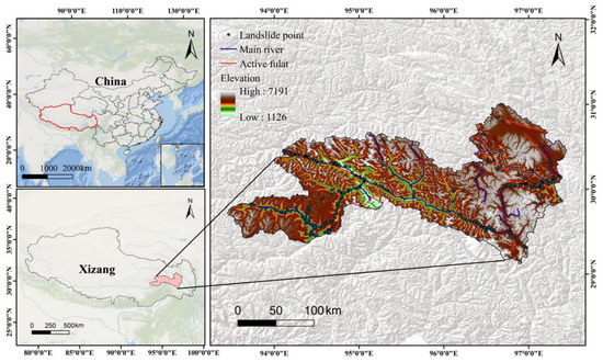
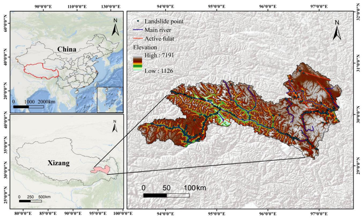
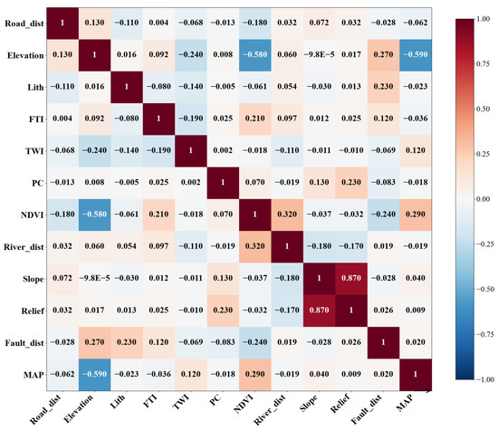
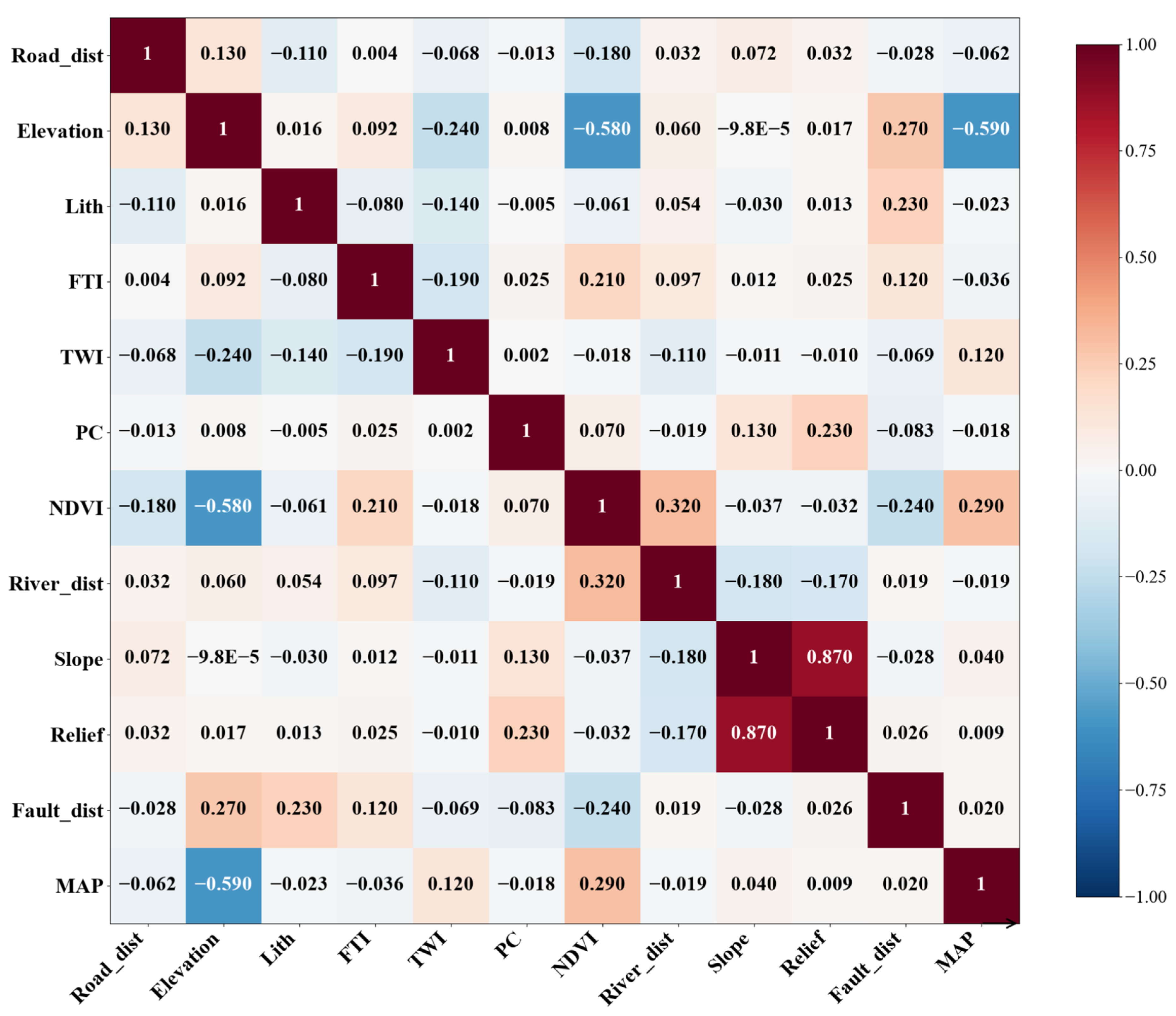
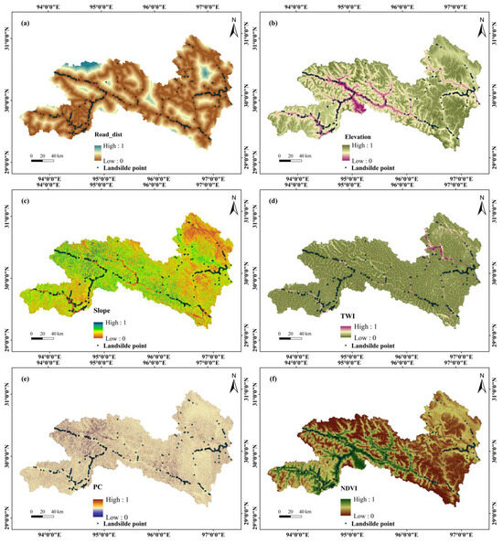
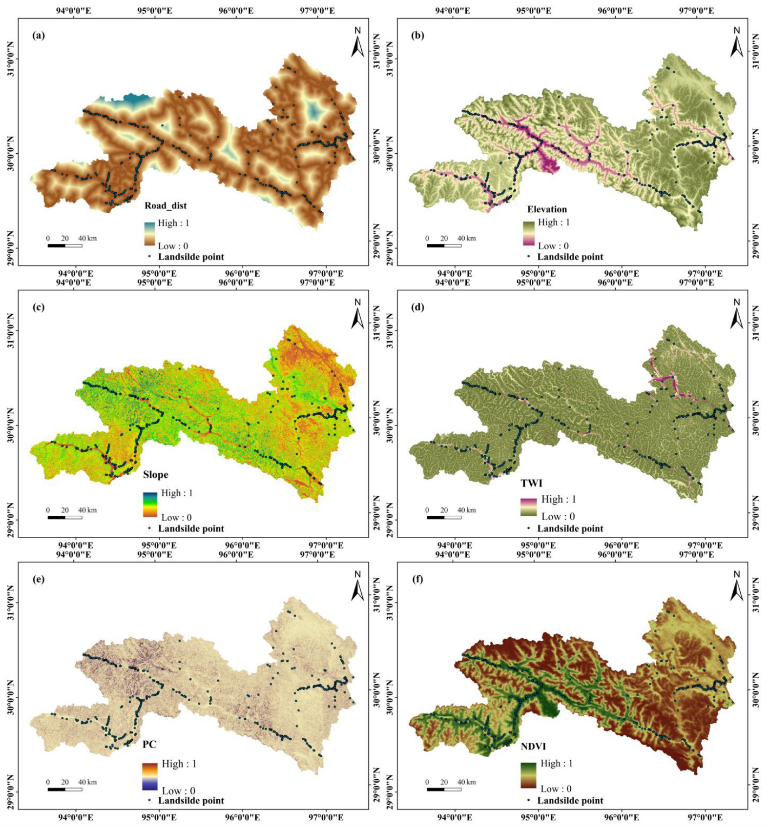
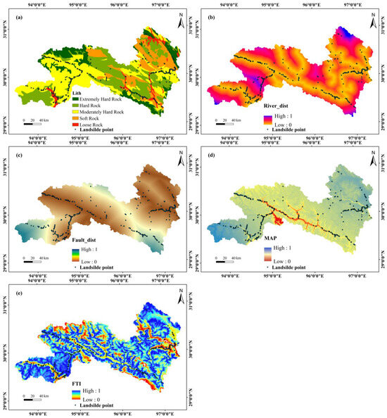
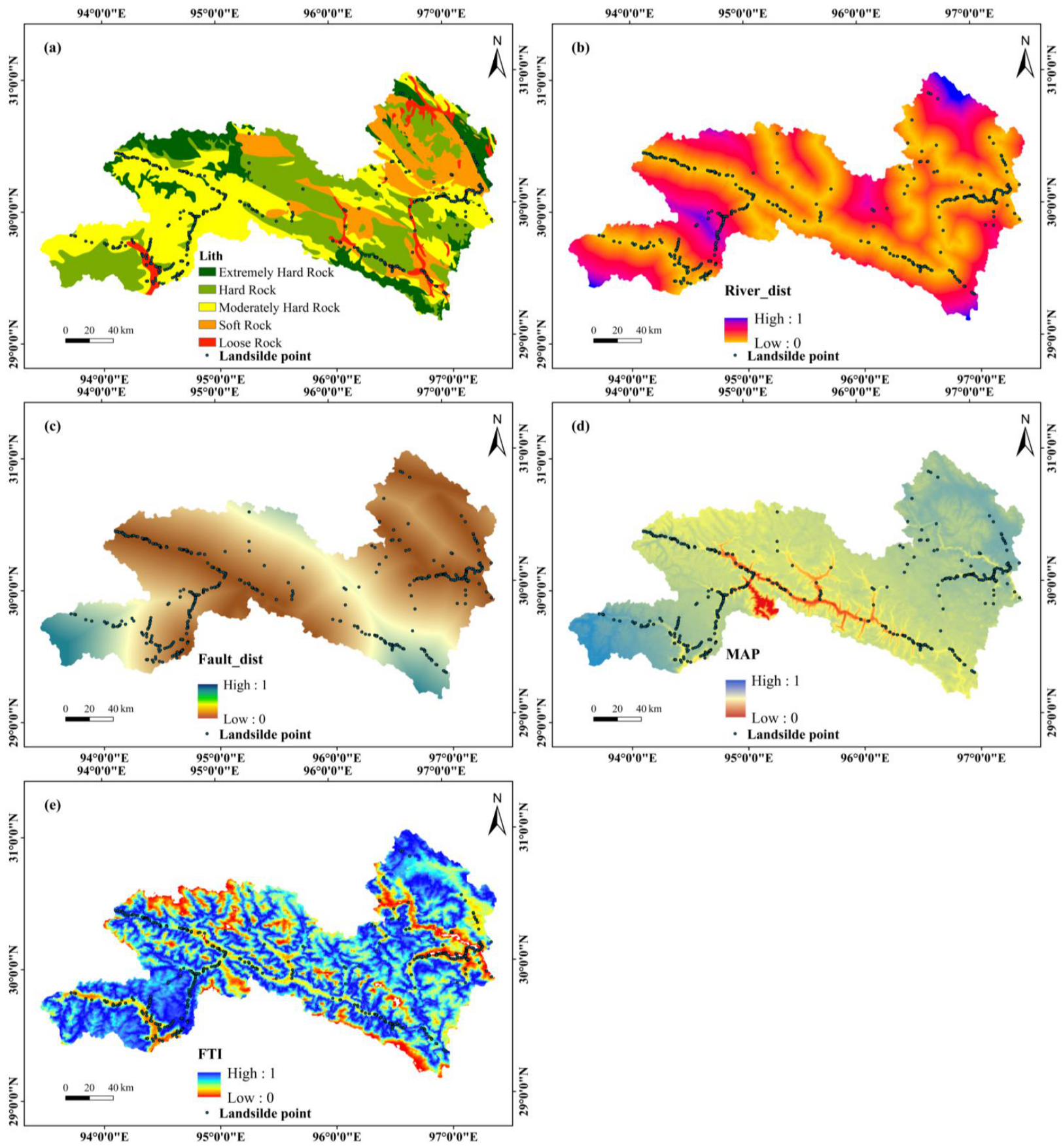
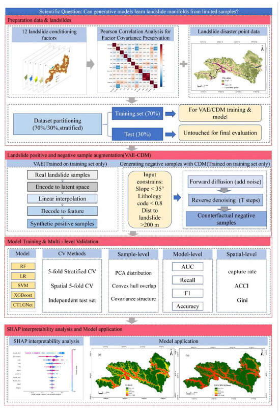
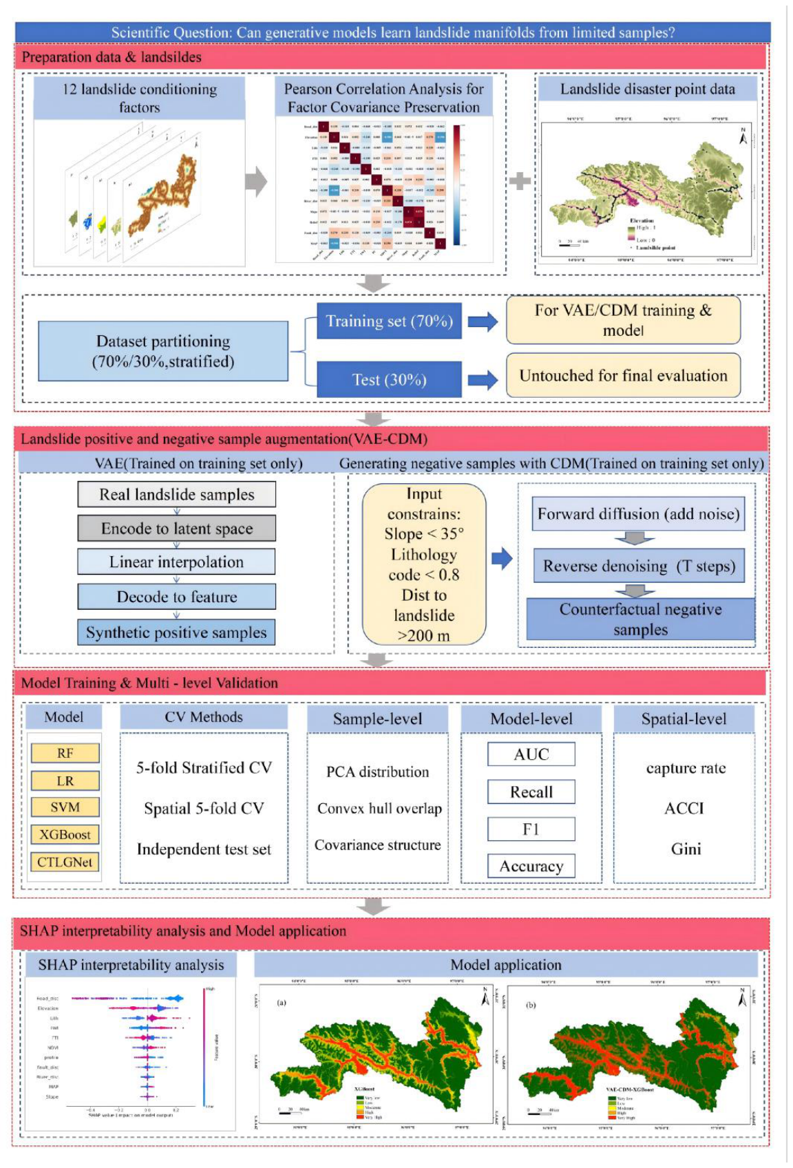
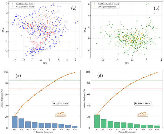
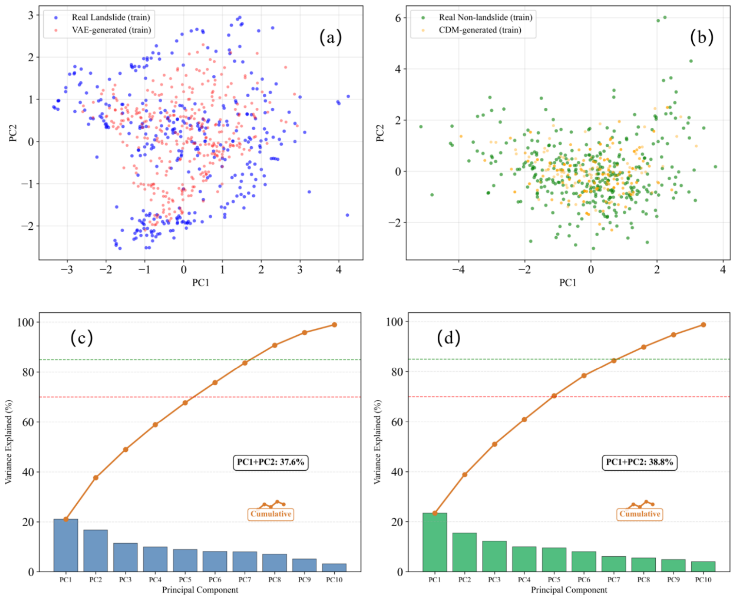
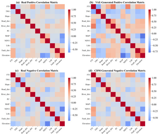
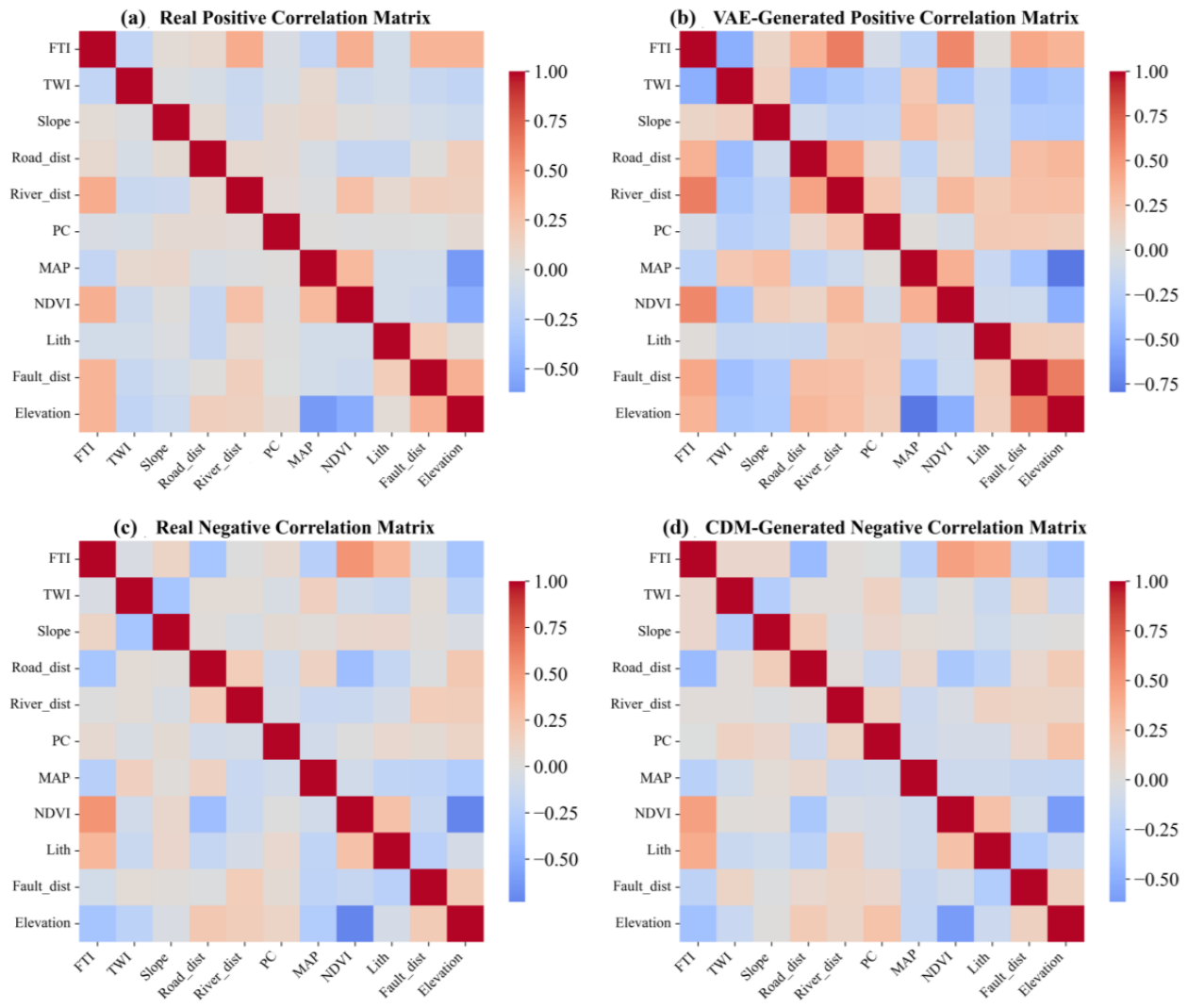
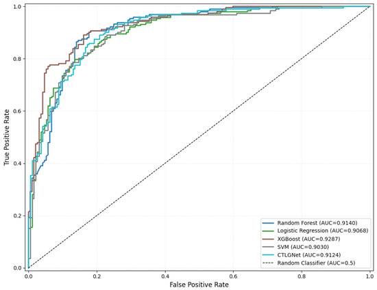
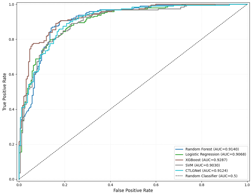
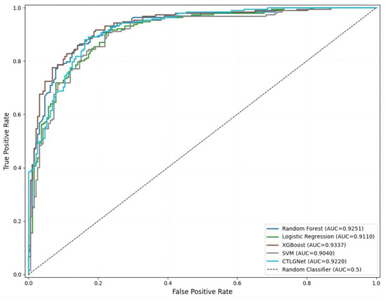
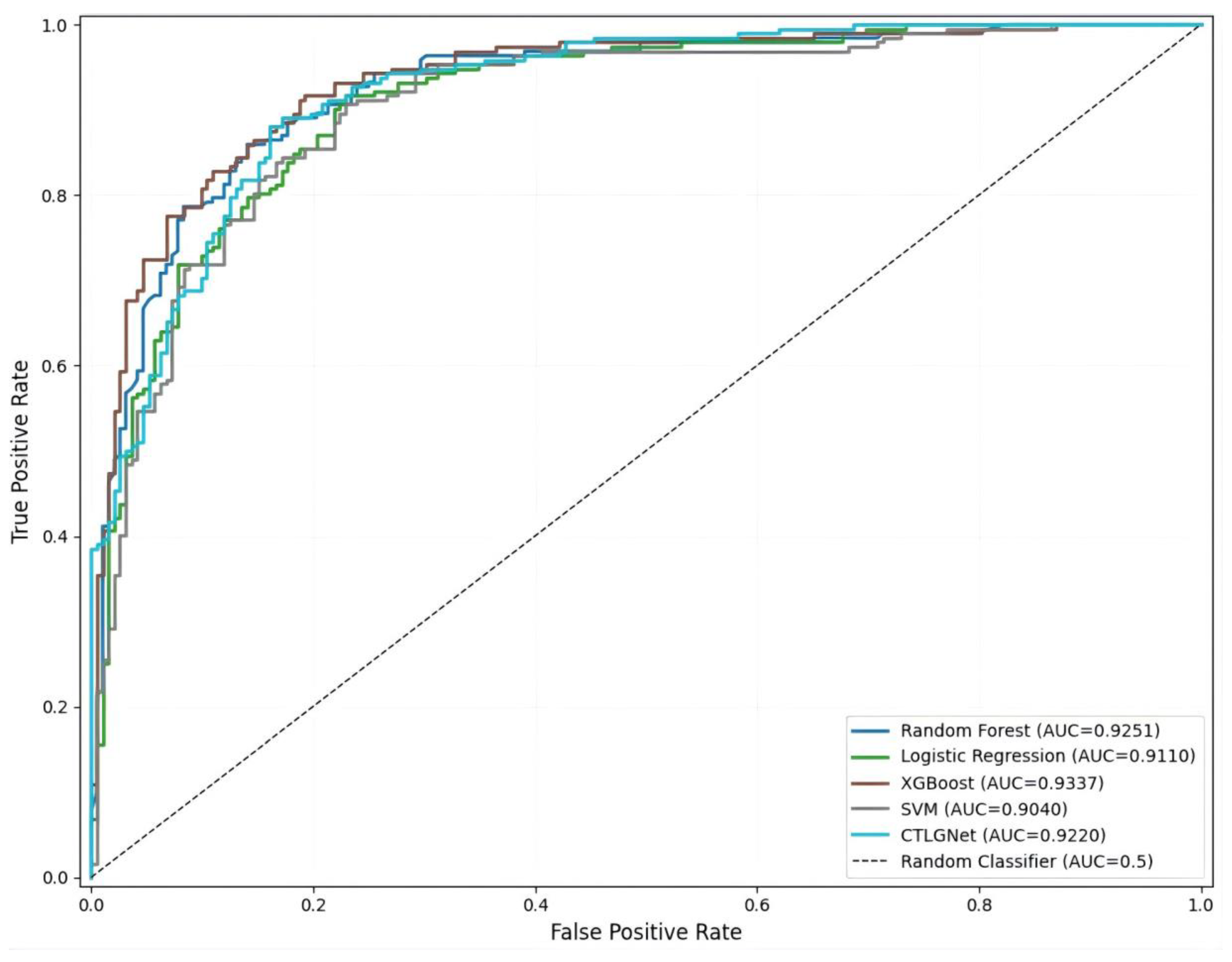
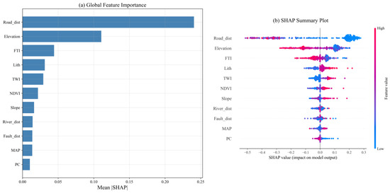
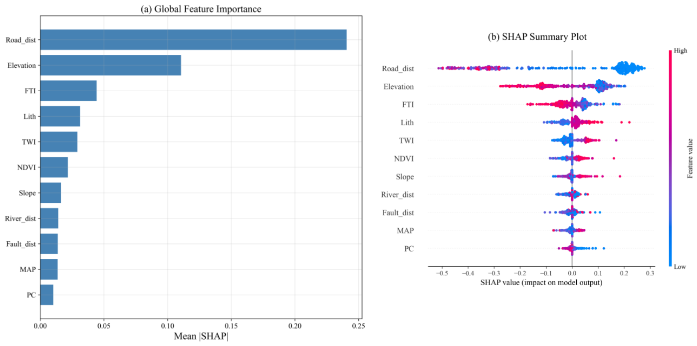
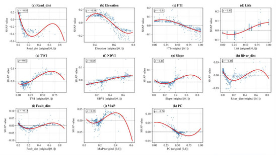
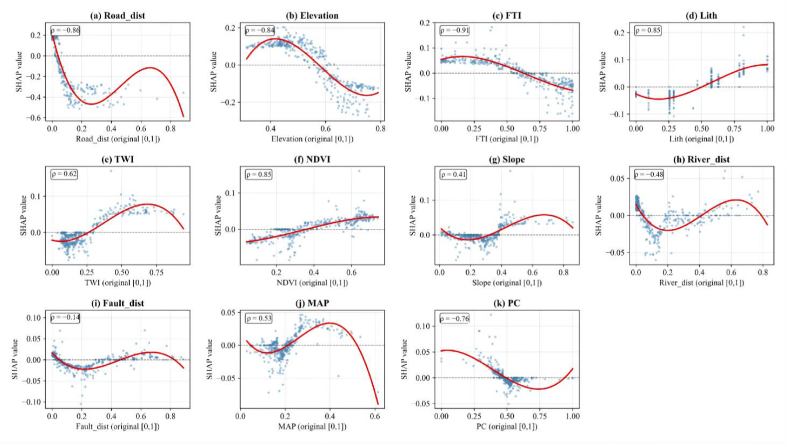
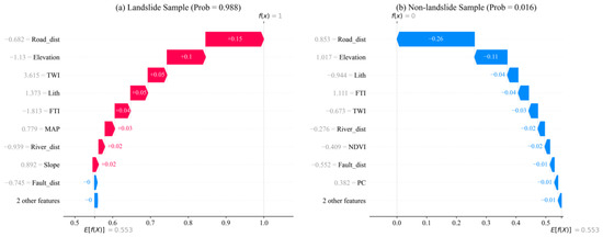
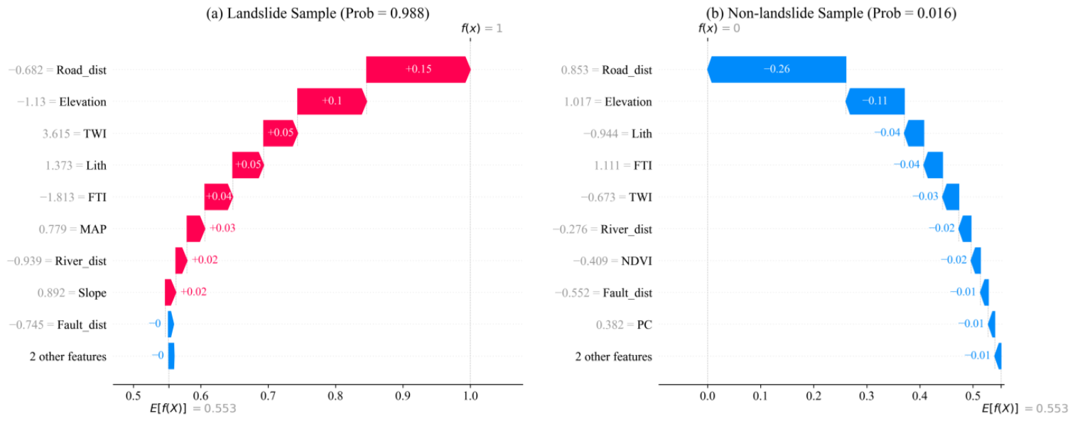
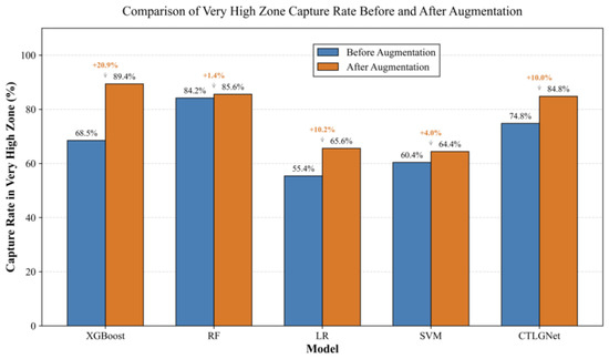
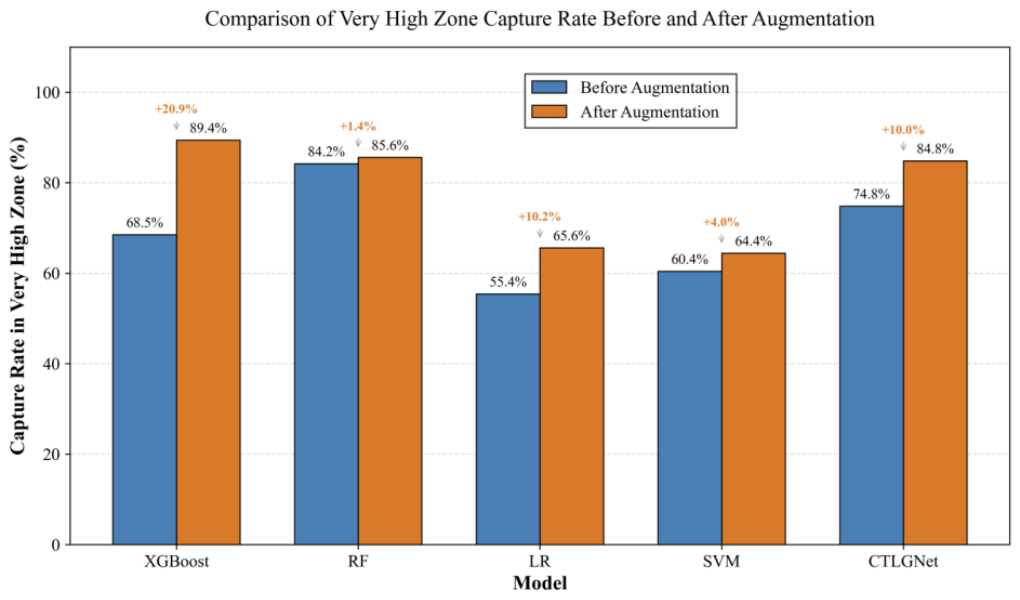
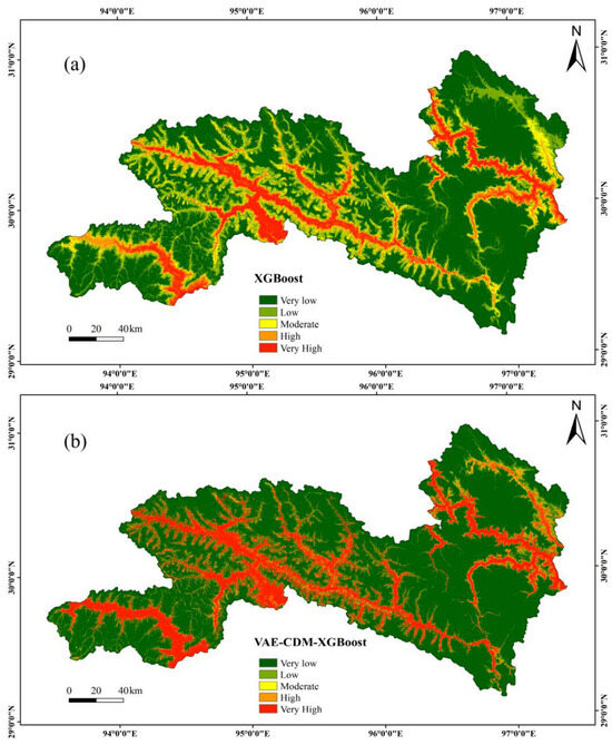
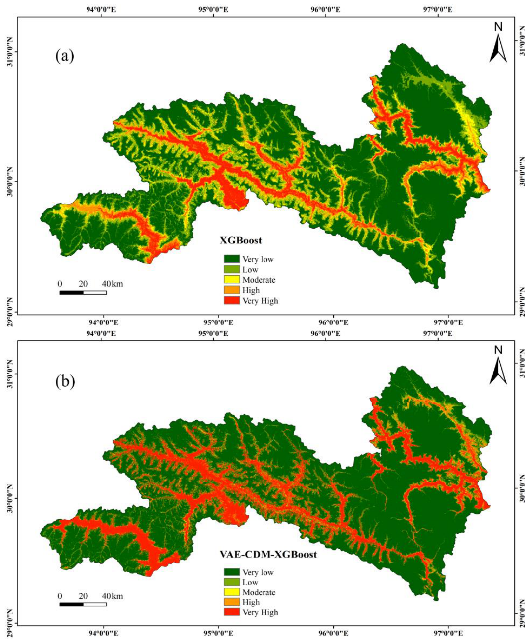
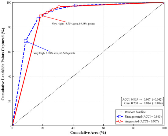
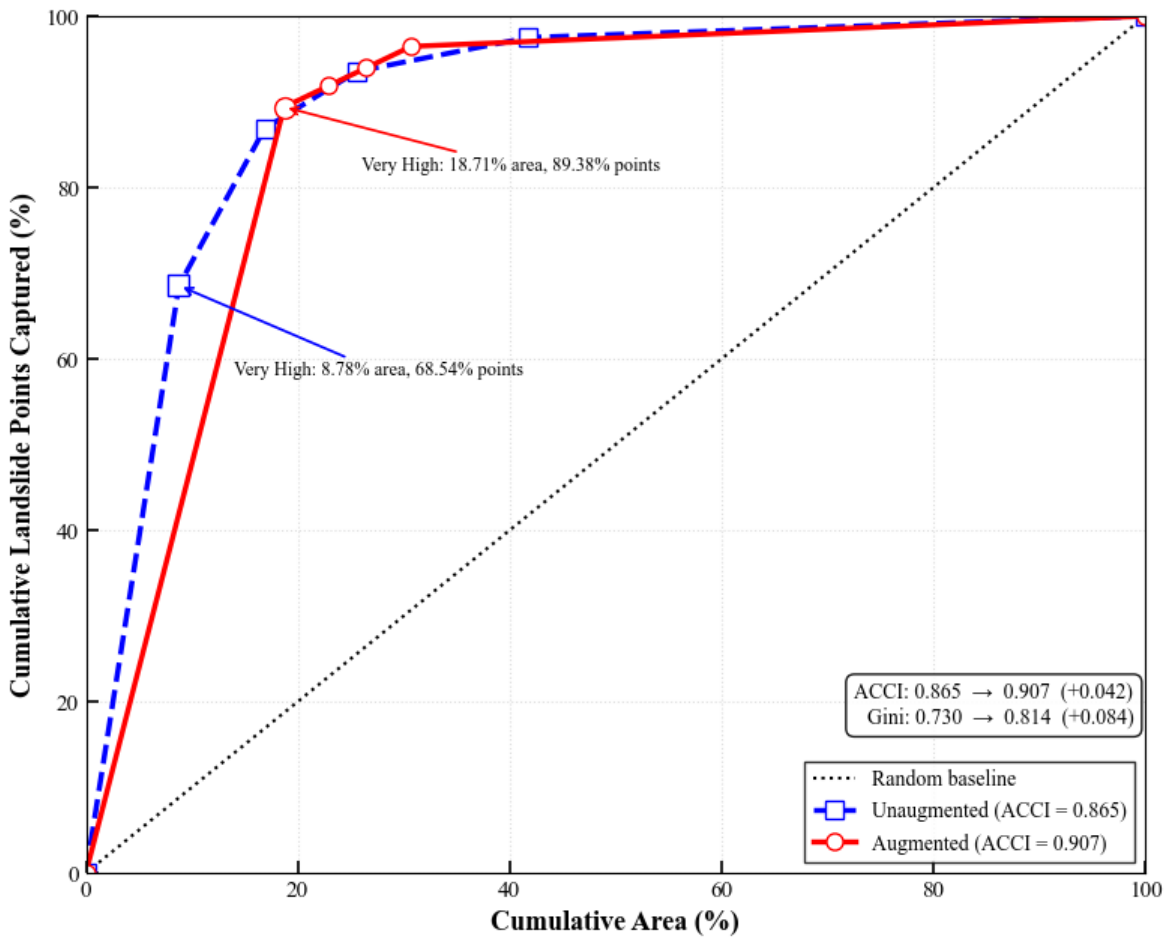

Disclaimer/Publisher’s Note: The statements, opinions and data contained in all publications are solely those of the individual author(s) and contributor(s) and not of MDPI and/or the editor(s). MDPI and/or the editor(s) disclaim responsibility for any injury to people or property resulting from any ideas, methods, instructions or products referred to in the content. |
© 2026 by the authors. Licensee MDPI, Basel, Switzerland. This article is an open access article distributed under the terms and conditions of the Creative Commons Attribution (CC BY) license.