


Abstract
The spring floods that occurred in 2024 in western and northern Kazakhstan caused extensive damage. Our understanding of runoff formation processes under frozen-soil conditions remains limited. In this study, we apply a coupled hydrothermal model as a case study to explicitly simulate vertical heat and water transport, phase transitions, snow dynamics, and reduced infiltration capacity due to cryogenic pore blockage (ice-filled pores). The model is based on regular meteorological data from 65 stations in five regions covering the full hydrological cycle (August–May) of 2021 and 2024. A multilevel diagnostic check showed that soil temperature is reproduced with a median of 0.962 and NSE of 0.888, the frozen/thawed surface condition corresponds to WMO (World Meteorological Organization) standards on approximately 91% of days, and water balance agreement reaches 86.2% (56 out of 65 stations). The model reflects the regional variability of the 2024 flood. In the northern regions (Kostanay, North Kazakhstan), snowfall was above average, and modeled runoff increased compared to 2021 (for example, at the Sergeevka station, it increased by a factor of four). In the western regions, the trends were mixed: the strongest relative increase in runoff was recorded in the Atyrau region (+119%), whilst in the West Kazakhstan region, the increase was more modest (+19%), and in the Aktobe region, runoff increased by 60%. The key mechanism—the time lag between rapid snowmelt and delayed soil thaw—is clearly evident: peaks in snowmelt occur when the soil remains frozen, infiltration capacity decreases, and the runoff potential index (RPI) exceeds 1 for extended periods. Although the model does not simulate the river channel, its ability to diagnose runoff generation conditions at the slope scale offers a diagnostic framework for identifying runoff-conducive conditions in regions with limited data, rather than a physically validated tool for flood-prone area identification. The results show that the 2024 flood period was characterized by abnormally high water inflow and hydrothermal conditions consistent with a temporal mismatch between water supply and the recovery of soil infiltration capacity. Because the RPI is a diagnostic indicator constructed from water input and infiltration capacity, these results should be interpreted as evidence of conditions conducive to runoff generation rather than as an independent causal verification of the flood mechanism.
Keywords:
floods; Kazakhstan; frozen soil; snowmelt; infiltration; hydrothermal modeling; timing mismatch 1. Introduction
In the spring of 2024, Kazakhstan was hit by a catastrophic flood, recognized as one of the most devastating natural disasters in the country’s history. A state of emergency was declared in 10 of the country’s 17 regions. According to official data, the flooding affected around 120,000 people, with more than 17,000 homes damaged [1].
According to the findings of emergency services and international experts, the key factors behind the flooding were abnormally high snow cover, extreme liquid precipitation during the snowmelt period, and increased pre-winter soil moisture [2,3]. At the same time, studies point to another important mechanism: the sharp warming at the end of March 2024 occurred against a backdrop of deeply frozen ground. Meltwater could not infiltrate downwards and was almost entirely transformed into surface runoff [4].
In the scientific literature, this effect is described as a temporary mismatch between the intense inflow of water to the surface and the persistence of low infiltration capacity due to the presence of interstitial ice. However, it should be emphasized that this explanation remains a scientific hypothesis requiring quantitative verification. Alternative mechanisms include predominantly sub-permafrost runoff, intra-permafrost filtration through melt channels, and combined processes, in which the dominant mechanism depends on the rate of spring warming and the initial depth of frost penetration.
Thus, the flood of 2024 poses a fundamental question for the hydrological community: what physical mechanism really determined the extreme runoff in various regions of Kazakhstan? Answering this question involves the application of a model tool tailored to diagnosing timing mismatch on a network of meteorological stations with a limited amount of input data.
In the existing literature, hydrological modeling of spring floods in cold regions has often relied on conceptual, semi-distributed, and land surface hydrological models, of which the most widely used are HBV, SWAT, and VIC. These models remain relevant in contemporary hydrological research: recent studies have applied or further developed HBV and VIC for parameter optimization and distributed modeling, while SWAT and HBV continue to be used for comparative streamflow estimation in data-limited basins [5,6,7].
The HBV model [8] uses degree-day formulations for snowmelt and empirical runoff generation functions. Its strength lies in computational simplicity and low data requirements, which makes it suitable for long-term forecasting and regional hydrological applications. However, in many applications, frozen-soil effects are represented only indirectly, for example, through air-temperature thresholds or empirical correction factors. This limits the ability of the model to diagnose abrupt reductions in infiltration capacity caused by pore-ice blockage. The SWAT model [9] includes a more detailed snow module and can estimate soil temperature in several layers, but the reduction in infiltration under frozen-soil conditions is commonly represented by empirical parameterization rather than by explicit ice-dependent hydraulic conductivity. The VIC model [10] implements an energy balance approach to snowmelt and represents heat transfer in the soil column; nevertheless, the influence of ice on hydraulic properties is usually simplified. Therefore, although HBV, SWAT, and VIC are effective for many streamflow and snowmelt applications, they are not primarily designed as diagnostic tools for identifying cryogenic infiltration blockage at the level of individual meteorological stations.
More physically detailed representations of freezing and thawing processes have been developed within cryogenic hydrology, soil physics, and geocryology. Established tools include SHAW, CoupModel, HYDRUS-1D, and more recent distributed hydrothermal coupling frameworks. The SHAW model [11] solves coupled one-dimensional heat and water transfer in the snow–residue–soil system and explicitly represents freezing and thawing processes. Recent modifications of SHAW have further improved the simulation of soil hydrological processes under freeze–thaw conditions by considering soil deformation and its effects on hydrothermal properties [12]. CoupModel [13] provides a flexible one-dimensional platform for coupled water, heat, carbon, and nitrogen processes and allows detailed configuration of soil freezing parameters. HYDRUS-1D with freezing modules [14,15] simulates coupled water, vapor, and heat movement during freezing–thawing periods and is widely used for detailed profile-scale analysis of frozen-soil processes. Recent thermal–hydro-mechanical formulations also demonstrate that coupled modeling of heat transfer, water infiltration, and deformation in frost-susceptible soils is already well established [16]. In addition, the DHTC model represents a modern distributed hydrothermal coupled hydrological framework for cold regions [17].
Thus, freeze–thaw hydrothermal coupling itself should not be regarded as a new concept. Existing cryogenic models provide high physical detail, but they are often designed for site-specific studies, require detailed soil-profile parameterization, or depend on spatially distributed information and calibration data that are not always available for regional station network diagnostics. Conversely, conceptual and semi-distributed hydrological models are easier to apply regionally, but their treatment of frozen-soil infiltration limitation is often simplified or indirect.
Table 1 compares the main model classes according to their treatment of snowmelt, freezing and thawing, ice-related infiltration reduction, connection to runoff, and data or computational requirements.
Table 1.
Comparison of model classes used to analyze spring flooding in cold regions.
The comparison shows that the proposed approach lies between highly simplified hydrological models and physically detailed cryogenic profile models. It does not aim to replace SHAW, CoupModel, HYDRUS-1D, DHTC, or fully distributed hydrological models. Instead, it is intended as a computationally simple diagnostic framework for identifying runoff generation conditions under limited data availability. Studies using physically based watershed models, including SWIM-based applications for spring floods in Kazakhstan [18], demonstrate the value of basin-scale modeling for analyzing cold-region runoff formation. However, such models are designed primarily to reproduce integrated catchment response, whereas this study focuses on diagnosing local infiltration limitation and timing mismatch at the meteorological station scale.
It is important to emphasize that the approach proposed in this study should be understood as a regional diagnostic case study rather than a novel modeling framework. The individual physical components—enthalpy-based phase-change representation, Richards-type moisture transfer, van Genuchten–Mualem hydraulic functions, and cryogenic impedance—are well-established and implemented in SHAW, CoupModel, HYDRUS-1D, and Noah-MP. Freeze–thaw hydrothermal coupling is not a new concept.
The contributions of this case study are application-specific and comprise three elements: (1) first, the simultaneous diagnostic application to 65 Kazhydromet meteorological stations across five regions of Kazakhstan with regional pedotransfer parameterization from the Kazakhstan state soil map; (2) the quantitative station-level testing of the timing mismatch hypothesis for the 2024 event—proposed qualitatively [4] but never tested across a regional network; and (3) the novel use of WMO KN-01 soil condition codes as deterministic autumn soil moisture initialization constraints.
Thus, the proposed model should be interpreted as a limited-data diagnostic tool rather than as a fully distributed flood-routing model. Its purpose is to identify where and when rapid snowmelt and liquid precipitation coincide with delayed recovery of soil infiltration capacity, thereby creating conditions favorable for surface runoff generation. Based on its application to 65 meteorological stations in the Atyrau, Aktobe, West Kazakhstan, Kostanay, and North Kazakhstan regions for the cold hydrological cycles of 2020–2021 and 2023–2024, the framework enables quantitative assessment of the timing mismatch mechanism during the 2024 extreme flood period.
2. Materials and Methods
2.1. Study Area and Data
In this paper, we examine the five regions of Kazakhstan most affected by spring floods in 2024: Atyrau, Aktobe, West Kazakhstan, Kostanay, and North Kazakhstan. The study area spans from 46° N to 55° N and from 48° E to 78° E, with stations unevenly distributed across these administrative territories (Table 2, Figure 1).
Table 2.
Geographic coordinates of the study area and meteorological station distribution by administrative region.
Figure 1.
Map of meteorological stations across the territory of Kazakhstan. Study regions: West Kazakhstan, Atyrau, Aktobe, Kostanay, and North Kazakhstan.
The territory is characterized by a sharply continental climate with pronounced latitudinal zonation: the average January temperature ranges from −5 °C in the southwest (Atyrau region) to −19 °C in the north of the region. Stable snow cover persists from November to March, and its average long-term height increases naturally along the latitude gradient from the low-power snow cover of the desert zone to the more stable and high snow cover of the forest–steppe and steppe zones [19].
We used the daily data of 65 meteorological stations of RSE Kazhydromet for the period from August to May 2020–2021 and 2023–2024 [20]. These two hydrological cycles (2020–2021 and 2023–2024) were deliberately chosen to test the central hypothesis of this study. The 2020–2021 cycle represents a background (relatively low-water) period in which spring snowmelt did not lead to extreme flooding. Conversely, the 2023–2024 cycle corresponds to a catastrophic historical flood—the most severe in recent decades. A systematic comparison of these two contrasting modes allows us to test whether the timing mismatch mechanism consistently distinguishes between flood and non-flood years. The 2024 flood is unique in recent history, and the availability of consistent soil condition codes (WMO KN-01) and meteorological data from the Kazhydromet network for these two periods ensures a robust comparison. While a longer time series would be desirable for generalization, the extreme contrast between these two years provides a strong test of the proposed mechanism. The database contains data on air temperature, soil surface temperature, soil surface condition codes, snow cover height, degree of snow cover, and precipitation.
To account for the influence of terrain on the formation of slope runoff, the SRTM (Shuttle Radar Topography Mission) digital terrain model with a resolution of 30 m was used, obtained through OpenTopography [21]. A local slope was calculated for each weather station in the km window (, Equation (15)), and used in the equation for laminar flow velocity.
To parameterize the roughness of the underlying surface, we used annual data from the MOD44B (Vegetation Continuous Fields) product of the MODIS satellite (NASA) with a spatial resolution of 500 m [22]. Based on the percentage of open soil (Percentage Non-Vegetated) for each time interval (2021 and 2024), the proportion of projective vegetation coverage () was calculated: . The obtained values of were used to calibrate the hydraulic resistance coefficients.
Short omissions of weather data (1–3 days) were restored by holding the last known value. Prolonged omissions led to the exclusion of the corresponding periods from the analysis. The total share of passes at all stations did not exceed 5%.
2.2. Model Description
Note that the model was operated in diagnostic mode throughout this study. The optional hydraulic routing component (laminar surface flow with vegetation resistance) was implemented in the code but not activated here, as the study objective was to estimate runoff generation potential rather than simulate flood propagation or channel flow. The model used in this case study was built on the van Genuchten [23] hydraulic functions and mass-conservative numerical scheme of Celia et al. [24], supplemented with coupled heat transfer accounting for cryogenic pore blockage () and a diagnostic runoff index (RPI) specifically designed to quantify the timing mismatch between snowmelt and soil thawing.
Hydrothermal processes were simulated continuously over the entire hydrological year on a 1.0 m vertical column ( m) [24] using a sequential operator-splitting scheme (Section 2.6), in which the heat-transfer equation was solved implicitly and the moisture equation explicitly.
Humidity fields in late autumn form the initial conditions of the system before winter freezing, and the cryogenic profile of ice pores accumulated over the winter acts as a limiter of infiltration and influences modeled runoff-generation potential in spring [25]. The model is diagnostic and mechanism-oriented. It focuses on isolating the timing mismatch (desynchronization) between the supply of meltwater and the infiltration capacity of the soil, rather than on a full hydrodynamic simulation of flood propagation or river routing [23,26].
The unsteady vertical distribution of the soil temperature field (°C) is described by a nonlinear thermal conductivity–convection equation modified for a partially frozen porous matrix:
where T is the soil temperature (°C), t is time (s), z is the vertical depth (m), is the effective volumetric heat capacity (), is the effective thermal conductivity (), and are the volumetric liquid water and ice contents (), and are the density () and specific heat () of liquid water, and is the downward water flux ().
Table 3 lists all input variables used by the model for each weather station.
Table 3.
Model inputs.
Figure 2 presents the general scheme of the modeling implementation.
Figure 2.
Conceptual framework of the coupled hydrothermal model, illustrating the interactions between snowmelt, soil freezing/thawing, infiltration limitation, and surface runoff generation through the timing mismatch mechanism.
The following sections detail the key components of the model: the method of effective heat capacity, the calculation of the moisture-dependent thermal conductivity, the cryogenic mechanics of infiltration and soil parameterization, the numerical scheme, the boundary conditions, and the formation of surface runoff and diagnostic indices (RPIs).
2.3. Effective Heat Capacity Method (Enthalpy Form)
To strictly comply with the law of conservation of energy during water–ice phase transitions, the system includes an effective heat capacity method within the finite range of the freezing point depression , which depends on the textural class of the soil (Table 4): for sands (Atyrau region), °C is assumed; for sandy loam (West Kazakhstan region), °C; for light loam (Aktobe region), °C; for medium loam (Kostanay region), °C; and for heavy loam (North Kazakhstan region), °C. This regional separation is due to the different ability of finely dispersed soils to retain unfrozen water and a wider interval of phase transition in clay soils.
where is the total porosity of the soil in the studied region, is the volume of liquid water, is the volume of intrapore ice, kg/m3 and J/(kg·K) are the density and heat capacity of ice, respectively, J/(m3·K) is the volumetric heat capacity of the mineral skeleton of the soil, and J/kg is the latent heat of melting.
Table 4.
Hydro- and thermophysical parameters of the pore matrix and textural classes of the study regions.
Enthalpy derivative (with regional ) functions as a nonlinear sink/energy source that iteratively absorbs or releases heat pulses during winter thaws and spring snowmelt, enabling the temperature of the calculation node to be maintained near the plateau of K until the phase transformation of moisture finalizes.
At subzero temperatures, , liquid humidity decreases to the residual value of , and ice fills the remaining pore volume: . In the transition zone (), the liquid and solid phases are distributed linearly depending on temperature. This ensures realistic seasonal freezing and thawing, which directly affects the infiltration capacity.
2.4. Moisture-Dependent Thermal Conductivity of the Soil
The dynamic volumetric thermal conductivity of the soil [W/(m·K)] is recalculated at each macro-step using the Coté and Konrad method [27] with the normalized Kersten number ():
where and are the thermal conductivity of dry and water-saturated soil, which are determined individually for each texture class (Table 4) and Kersten number . The coefficient 1.1 multiplied by the volume content of ice () in the thermal conductivity formula reflects the ratio of water density to ice density (), which is necessary to correctly account for the volume of pores occupied by ice.
2.5. Cryogenic Mechanics of Infiltration and Soil Parameterization
The vertical redistribution of moisture in unsaturated conditions is described by the Richards equation in mixed diffusion–gravity form, taking into account the cryogenic reduction in hydraulic conductivity:
where is the effective moisture diffusivity, is a characteristic capillary length scale ensuring dimensional consistency, is the hydraulic conductivity, calculated using the van Genuchten model [23] with cryogenic correction (Equation (6)), and is the phase-change mass source term (Equation (7)). Equation (4) is therefore a Richards-type, mixed diffusion–gravity approximation, in which the capillary diffusion term uses a constant length scale rather than the full soil-water diffusivity . The first term represents moisture diffusion driven by the matric potential gradient, and the second term represents gravitational drainage, which is the dominant flux mechanism when the soil approaches saturation during spring snowmelt. At cell interfaces, hydraulic conductivity is evaluated as the arithmetic mean of adjacent nodes: . This represents downward gravity-driven flow under near-saturated conditions typical of spring snowmelt on frozen soils.
2.5.1. Closure According to the Mualem–Van Genuchten Model
Hydrophysical functions are closed using the fundamental Mualem–van Genuchten parameterizations model [23]:
where and —effective saturation of pores with liquid water. This parameter is calculated strictly relative to the available free porosity, reduced by the current volume of intrapore ice . The dimensionless coefficient of cryogenic impedance is assumed to be in strict accordance with the validated equations of hydrodynamics of frozen media embedded in the global climatic and hydrological models SHAW [11] and Noah-MP [28].
As pore ice content increases, the hydraulic conductivity decreases exponentially through the cryogenic impedance term in Equation (6), reflecting progressive pore blockage and increased flow tortuosity. For the soil textures considered here (), this formulation predicts a reduction in hydraulic conductivity of approximately 50–53% when the ice-filled pore fraction reaches , and approximately 75–78% when it reaches .
2.5.2. Pedotransfer Coordinate Reference Procedure
In order to exclude the subjective selection of empirical coefficients, a strict Pedotransfer Mapping Procedure was implemented as part of a numerical experiment. The state soil map of the Republic of Kazakhstan has been digitized and verified by converting it to the USDA International Classification of texture classes (based on validated granulometric composition matching matrices).
The identified regional study areas were compared with the reference physical base of the Carsel and Parrish constants [29] (Table 4), which allowed us to form invariant physical profiles of the model, free from stochastic parameter fitting.
2.5.3. Phase-Change Mass Coupling
To ensure mass conservation during freeze–thaw events, the moisture balance Equation (4) includes a source term that accounts for the conversion of ice to liquid water is as follows:
where and (m3/m3) are the volumetric ice contents at the previous and current time steps, respectively, and (s) is the hourly moisture time step ( s). The operator ensures that only ice melting contributes as a liquid water source; refreezing is handled separately by the phase transition boundary in the ice content update procedure. This approach follows the operator-splitting treatment of coupled heat–moisture systems described in [14] and ensures that meltwater produced by the thermal block is correctly transferred to the hydrological block at each time step, preserving mass conservation during spring thaw events.
2.6. Discrete Numerical Time-Splitting Scheme
The conjugate nonlinear system is solved using the finite difference method, which involves splitting through physical processes and a time-splitting technique [24]. This method employs a division based on two independent spatial scales:
- 1.
- Vertical soil column with a depth of 1 m with a uniform step of m (20 nodes). On this grid, the implicit scheme (daily step s) solves the heat transfer equation with phase transitions, and the explicit scheme (hourly step s) solves the Richards equation for moisture transfer. The column represents a local point (elementary catchment area) and calculates the temperature profile, ice content, infiltration capacity, and water balance.
- 2.
- A horizontal slope area measuring km, for which the local slope is calculated according to SRTM data. This parameter is used only in the parameterization of the laminar flow rate of excess water and does not require spatial sampling.
The sequential operator-splitting strategy introduces a coupling error of order in the energy–mass exchange. To minimize this error, three measures are implemented: (1) All temperature-dependent hydraulic properties (, , ) are recalculated at the start of each daily macro-step from the updated and fields; (2) the phase-change mass source is explicitly transferred from the thermal block to the moisture block at each macro-step; and (3) hydraulic conductivity is updated at each hourly micro-step within the nested moisture loop.
This pseudo-implicit coefficient update strategy substantially reduces the effective splitting error and follows the approach applied in the Noah-MP land surface model [28]. The residual splitting error is acceptable for the diagnostic purpose of identifying timing mismatch conditions, as confirmed by the validation results presented in Section 3.3.
Since the flow hydraulics are not directly modeled, but only the potential for surface runoff formation is estimated, the vertical soil column and slope section do not require strict spatial coordination. The difference in grid scales does not lead to numerical inconsistency, since the models are connected through a common physical criterion for the transition to surface runoff. This approach allows us to focus on the key mechanism—the time discrepancy between snowmelt and soil thawing (timing mismatch).
Time integration is performed with different steps for different processes: the thermal block is solved with an implicit finite-difference scheme of the first order in time and the second order in space at the daily macro-step s, which ensures unconditional stability. The Richards equation for moisture transfer is solved using an explicit scheme with an hourly step of s, and surface runoff is calculated using an explicit scheme with a step of s, satisfying the Courant–Friedrichs–Lewy (CFL) condition.
The space–time discretization of the equation of thermal conductivity and balance of phase transitions has the following form:
where is the effective heat capacity () at grid node i and time step n, is soil temperature (°C), is the macro-time step (s), is the vertical grid spacing, is the thermal conductivity ()) at the interface between nodes, is the infiltration flux (), and and are the density and specific heat of liquid water ( and J/(kg·K)).
To preserve second-order spatial accuracy, at the lower boundary of the soil column (), the ghost node () is eliminated by applying a second-order Neumann boundary condition within the central difference discretization. The resulting expression forms the final row of the tridiagonal system of linear algebraic equations:
In Equation (9), is the geothermal heat flux. The resulting system of linear algebraic equations has a tridiagonal form and is efficiently solved at each time step using the Thomas algorithm.
Within each daily macro-step, a nested iteration cycle is initialized at an hourly micro-step = 3600 s. This block performs a layer-by-layer recalculation of the dynamic redistribution of moisture according to the nonlinear Richards equation and routes the excess surface layer of water , strictly satisfying the criteria of numerical stability of CFL for explicit schemes.
2.7. Boundary Conditions
Dynamic variables of volumetric humidity () and ice content () at the beginning of the winter period are initialized deterministically by decoding the daily synoptic codes of the soil surface condition (Table 5) for October–November 2020 and 2023 [25]. This approach allowed us to identify the key hydrological triggers that caused the difference between the low-flow spring period of 2021 and the catastrophic flood of 2024.
Table 5.
Synoptic codes of soil surface conditions (WMO KN-01).
Soil codes 0–3 are taken into account in the autumn initialization, as they describe the moisture content of the open soil surface before freezing. Soil codes 4–9 already relate to winter phase states—frozen soil, ice, and snow; thus, they are used not to set the initial humidity, but to subsequently check the phase state of the surface.
Base scenario for 2021 (autumn 2020): The predominance of the soil codes of the dry and moderately moist upper layer (soil codes 0 and 1) fixes a significant deficit in the pre-winter moisture profile. In this case, the starting humidity is assumed to be close to the residual value: .
At the same time, the effective volume of intrapore ice tends to zero (), leaving the pore channels free for high-intensity spring infiltration.
Flood scenario of 2024 (autumn 2023): Continuous multi-day recordings of wet, waterlogged, and superficially flooded soils (soil codes 1–3, corresponding to moist soil) verify the extreme rise in water level immediately before the onset of stable negative temperatures. In this case, humidity is approximated at the level of full saturation porosity: .
Upon subsequent freezing, this volume of free moisture almost entirely passes into the solid phase (), forming a continuous cryogenic water barrier by the beginning of spring snowmelt.
2.7.1. Upper Bound ()
The upper thermal node of the computational grid is , which calculates the dynamic thermal resistance and thermal insulation effect of seasonal snow cover (, (m)):
where the exponential attenuation coefficient in the initial formulation is recalculated daily as a nonlinear function of snow density and metamorphism according to Sturm’s formulas [30], ranging from m−1 (winter dry wind snow) to m−1 (spring wet ripened snow). In the numerical implementation, due to the lack of daily measurements of snow density, the coefficient is assumed to be constant m−1, which corresponds to the average value and does not lead to a significant error in timing mismatch diagnostics.
The actual layer of meltwater entering the daytime surface in a calculated time step (, (m)) is calculated only at a positive air temperature ( °C), which eliminates the generation of false volumes of moisture from the winter settling of snowdrifts:
where is the daily volume of liquid precipitation, = 1000 kg/m3, and is the snow density, which in the model depends on the snow cover status code E′ (Table 6): for dry loose snow (E′ codes 5–8), = 150 kg/m3 is accepted; for wet packed snow (E′ codes 1–4), = 400 kg/m3; and for ice (E′ code 0), = 917 kg/m3.
Table 6.
Snow codes E′ (soil surface conditions in the presence of snow or ice cover) based on WMO FM-12 SYNOP code [25].
The actual rate of moisture infiltration into the soil profile () is limited by the current absorption capacity of the upper calculation node (): .
2.7.2. Lower Bound ( m)
The process of bidirectional thawing is modeled by setting a physically valid second-order Neumann boundary condition at the lower boundary of the domain. This condition reflects the stable upward geothermal heat flow of the Earth ( = 0.06 W/m2) for the Eurasian lithospheric plate:
In the hydrodynamic block at the lower boundary (), the condition of free gravitational drainage is set:
This methodological approach is mathematically the least arbitrary and introduces the so-called conservative error into the calculation scheme. By completely eliminating artificial moisture supports from below, this boundary condition helps isolate the modeled contribution of cryogenic pore sealing in the upper aeration zone to spring surface runoff, within the adopted model assumptions, rather than attributing runoff to marginal defects or boundary artifacts of the computational grid [24].
Short gaps (1–3 days) were filled in by retaining the last known value, and longer gaps led to the exclusion of the corresponding days from the analysis.
2.8. Hydrodynamics of Surface Slope Runoff
The infiltration capacity (mm/day) is dynamically computed at each daily time step from the effective hydraulic conductivity of the uppermost soil layer, which explicitly accounts for cryogenic ice blockage through Equation (6):
where is given by Equation (6), s, and the factor converts m/s to mm/day. As ice content in the surface layer increases during winter freezing, the cryogenic impedance factor causes both and to decrease exponentially—by approximately 75–78% when . Conversely, as the thawing front descends and decreases in spring, recovers progressively. This dynamic coupling between the thermal state, represented by from the enthalpy block, and the hydraulic state, represented by , constitutes the core physical mechanism of the timing mismatch hypothesis.
To account for the spatial heterogeneity of the relief, the dimensionless slope coefficient was calculated individually for each of the 65 weather stations using the SRTM 30m digital terrain model. An altitude window of km was cut out around the coordinates of the station, from which a local elementary slope was then determined:
where and (m) are the elevations at the upper and lower boundaries of the 1 × 1 km window centered on each meteorological station, and (m) is the horizontal distance between them.
2.9. Runoff Potential Diagnostic Index (RPI)
The Runoff Potential Index (RPI) was introduced to quantify the timing mismatch hypothesis:
where is the daily meltwater input calculated from the decrease in snow cover height, and is the daily liquid precipitation. When RPI > 1, the estimated daily water supply exceeds the infiltration capacity of the upper soil layer, indicating conditions favorable for surface runoff generation. RPI is therefore used as a diagnostic consistency indicator rather than as an independent validation metric. Because water input and infiltration capacity are explicitly included in its definition, exceeding the RPI threshold alone cannot be interpreted as diagnostic consistency of the proposed timing-mismatch mechanism. Instead, the index is used to compare the duration, timing, and regional synchronization of runoff-conducive conditions between the 2020–2021 and 2023–2024 hydrological cycles. For each station, changes in the number of days with RPI , total water inflow, and model runoff between the periods under consideration were calculated: , , and . The indicator characterizes changes in the duration of periods with a high potential for surface runoff formation, while and reflect changes in water inflow and catchment response, respectively.
Stations were classified according to the degree of diagnostic consistency. Strong consistency was assigned if both conditions of the hypothesis were fulfilled simultaneously: an increase in the number of days from RPI () and the signs and matched; partial consistency was assigned if only one of them was fulfilled. There were two conditions; if neither of the conditions were met, the station was classified as not consistent.
2.10. Diagnostic Validation Strategy
Direct observations of river discharge and flood extent were not available for all stations, and thus direct validation against observed discharge was not feasible due to the absence of gauging stations at the spatial scale of our elementary slopes and the unavailability of flood extent data for 2024. Thus, the model was evaluated using a multi-level diagnostic validation strategy, focusing on the hydrothermal state—the primary driver of runoff generation. This is a standard approach for diagnostic models that aim to identify conditions conducive to runoff rather than to simulate flood hydrographs.
The validation focused on hydrothermal parameters that directly control runoff generation: soil temperature (thermal regime of the active layer), frozen/thawed surface state (phase condition of the uppermost soil layer), infiltration capacity (influenced by ice content and soil texture), and water balance consistency (relationship between water input and modeled runoff). These parameters are the primary physical drivers of surface runoff formation in cold regions, rather than the flood hydrograph itself, which would require separate river route modeling.
Three levels of validation were used:
- 1.
- Comparison of the simulated near-surface soil temperature with observations of soil temperature at the station.
- 2.
- Comparison of the simulated frozen/thawed surface state with the WMO soil condition codes (KN-01).
- 3.
- Assessment of the consistency in the sign of change between total water inflow and modeled surface runoff when comparing 2021 and 2024.
These validation levels were chosen because soil temperature and phase state are the primary controls of infiltration capacity in frozen soils. The third level provides a diagnostic check on whether the modeled runoff response is physically consistent with changes in water input.
The following indicators were used: , the Nash–Sutcliffe efficiency coefficient (NSE), bias, and the phase state correspondence, defined as the proportion of days with the correct definition of the frozen/thawed surface. The consistency of the water balance was estimated as the proportion of stations where the sign of the change in the total water inflow between 2021 and 2024 coincides with the sign of the change in the model surface runoff (consistency coefficient).
3. Results
3.1. Interannual Consistency of Water Balance
For an initial assessment of the physical viability of the model, the relationship between changes in total water inflow and changes in model surface runoff between 2021 and 2024 was analyzed. Figure 3 shows the relationship between the change in the total seasonal water inflow (Input) and the corresponding change in runoff (Runoff) for the studied stations.
Figure 3.
Interannual agreement between changes in total water inflow and changes in runoff in 2021 and 2024. Green dots indicate stations consistent with the model’s hydrological response; red dots indicate inconsistent stations.
Most stations show a consistent response: an increase in water inflow was accompanied by an increase in model runoff, and a decrease in water inflow was accompanied by a decrease in runoff. A total of 56 out of 65 stations (86.2%) showed a consistent direction of change, which indicates a physically plausible interannual model response.
To facilitate spatial comparison, the station-based results were aggregated by region. Table 7 summarizes the mean total water input and simulated surface runoff for 2021 and 2024, together with their standard deviations and the results of paired t-tests.
Table 7.
Regional summary of model results for 2021 and 2024 (mean ± standard deviation across stations). Statistical significance was evaluated using paired t-tests.
To assess the robustness of regional differences, we calculated standard deviations (reported as mean ± standard deviation) across stations within each region and performed paired t-tests to evaluate the statistical significance of interannual changes between 2021 and 2024. The results show that increases in total water input were statistically significant () for all regions, although the effect was weakest in West Kazakhstan (). For modeled runoff, the increases were significant () in the Aktobe, Atyrau, Kostanay, and North Kazakhstan regions, but not in West Kazakhstan (). This suggests that, in West Kazakhstan, the increase in runoff was less pronounced and more variable across stations, likely due to the predominance of sandy loam soils, which freeze less deeply and thaw more rapidly, thereby reducing the cryogenic effect. The relatively large standard deviations indicate considerable spatial heterogeneity within all regions, reflecting differences in local snow accumulation, soil properties, and topographic conditions.
To assess the stability of the proposed mechanism, the stations were classified according to the degree of diagnostic consistency for the timing mismatch hypothesis. The classification results are shown in Table 8.
Table 8.
Regional distribution of diagnostic consistency for the timing mismatch hypothesis.
The hypothesis was diagnostically consistent across all studied territories: The consistency rate was 100% in four regions and 91.7% in the West Kazakhstan region. In the Kostanay, Aktobe, and Atyrau regions, all stations are classified as having strong consistency. In the North Kazakhstan region, 80% of stations have strong consistency and 20% have partial consistency, which gives an overall consistency of 100%.
In the West Kazakhstan region, consistency was 91.7%, and one station did not meet the hypothesis criterion. This may indicate the presence of local factors that affect the formation of runoff and are not taken into account by the mechanism under consideration.
It is important to distinguish between the RPI threshold condition and the scientific findings of this analysis. The RPI formula defines when runoff generation occurs (RPI when ). The scientific findings concern what is not embedded in this definition: (1) In 2024, all five regions reached peak RPI excess within a 6-day window (2–8 April), driven by a documented large-scale synoptic warming event on 1–2 April, whereas in 2021, peaks were distributed over 19 days (25 March–13 April)—this spatial synchronization explains the catastrophic scale of the 2024 event. (2) The pre-winter soil moisture state (wet autumn 2023 vs. dry autumn 2020) determined the initial ice content and thus the spring suppression. (3) Stations in the Ural River floodplain (Uralsk: mm; Chapayevo: mm) show negative , correctly reflecting that their 2024 flooding was driven by river overflow rather than slope-scale runoff generation—consistent with the diagnostic scope of the model.
3.2. Coupled Hydrothermal Evolution on the Example of the Sergeevka Station
After a regional generalization, a detailed example of the Sergeevka station (North Kazakhstan region) was considered. Figure 4 shows the conjugate evolution of water inflow, frozen layer, infiltration capacity and potential runoff index (RPI) in the cold season of 2023–2024.
Figure 4.
Coupled hydrothermal evolution at the Sergeevka station (North Kazakhstan region) during the 2023–2024 cold season: (a) water input (snowmelt and precipitation), (b) frozen layer thickness, (c) infiltration efficiency, (d) runoff potential index (RPI). Vertical dashed lines indicate key transition dates: green—onset of snowmelt, orange—peak snowmelt. The horizontal gray dashed line in panel (d) indicates the runoff potential threshold (RPI = 1).
The results show that during the cold season of 2023–2024, the Sergeevka station experienced a temporary overlap of water inflow, frozen soil conditions, and reduced infiltration capacity. Some of the snowmelt and precipitation impulses occurred against the background of a persistent frozen layer, especially in the autumn–winter and early spring periods. At this time, infiltration efficiency remained low, accompanied by a higher threshold value of , which is indicative of a greater probability of surface runoff formation.
At the same time, the main peak of snowmelt in early April falls in the transition stage, when the frozen layer was already beginning to degrade and the infiltration capacity was rapidly restored. This shows that the mechanism of runoff formation is related to not only the presence of a frozen layer but also the temporary discrepancy between the flow of water, the condition of the soil, and the rate of infiltration recovery.
In 2024, rapid spring warming led to intense snowmelt. However, the soil remained frozen at depth, as thawing takes longer. As a result, the infiltration capacity was significantly reduced, which resulted in exceedance of the RPI threshold, indicating conditions conducive to surface runoff generation—a modeled example of the timing mismatch mechanism.
Thus, the key result is not just the coincidence of snowmelt and freezing maxima, but the presence of a transition period when the water inflow increases faster than the soil has time to restore its infiltration capacity. This temporal discrepancy is consistent with the proposed timing mismatch mechanism.
In order to identify the most pronounced model reactions, a table of stations with the largest absolute change in surface runoff between 2021 and 2024 was compiled.
Table 9 shows that changes in modeled surface runoff between 2021 and 2024 were concentrated mainly at stations located in the North Kazakhstan and Kostanay regions. The largest increase in modeled runoff was calculated for the Saumalkol station, where the difference between 2021 and 2024 reached +304 mm. High runoff increases were also obtained for the Arshalinsky Z/SVH, Zhitikara, Mikhaylovka, and Karabutak stations.
Table 9.
Stations with the greatest modeled change in surface runoff between 2021 and 2024.
In most cases, an increase in surface runoff was accompanied by an increase in the number of days exceeding the threshold of . This indicates longer periods of potential surface runoff generation in 2024 compared with 2021. However, this relationship was not observed at all stations. For example, at Mikhaylovka station, the number of days with decreased by 22 days, despite a substantial increase in total modeled runoff. This demonstrates that flood response intensity is controlled by not only the duration of threshold exceedance but also the magnitude of the water pulse and its coincidence with periods of reduced soil infiltration capacity.
The case of the Mikhaylovka station warrants particular attention because it represents an apparent paradox: modeled runoff increased by 226 mm between 2021 and 2024, while the number of days with decreased by 22 days. This apparent inconsistency can be explained by considering the intensity rather than only the frequency of RPI exceedance events. In 2024, Mikhaylovka experienced fewer but substantially more intense snowmelt pulses. Total water input increased by 285 mm (41.5%), with additional water concentrated within a short period of rapid spring warming. During this period, the soil remained frozen and infiltration capacity was strongly reduced. Consequently, a single large meltwater pulse produced more runoff than multiple smaller pulses distributed over a longer period in 2021.
This observation highlights an important limitation of using the number of days with as a standalone indicator. While the duration of threshold exceedance reflects the persistence of flood-prone conditions, the magnitude of daily water surplus is equally important. Total runoff is determined by the temporal integration of RPI exceedance, rather than by exceedance frequency alone. Therefore, the Mikhaylovka response is consistent with the timing mismatch mechanism: the critical factor is not the number of days when the threshold was exceeded, but whether the largest water pulses occurred during periods of minimum infiltration capacity.
Thus, the results for individual stations confirm that the strongest model response was formed not only due to an increase in total water intake, but also due to an unfavorable combination of snowmelt, precipitation, and the limited infiltration capacity of frozen soil.
3.3. Thermal Structure of the Soil and Dynamics of the Thawing Front
For an additional physical explanation of the revealed mechanism, the vertical structure of the ground temperature at the Sergeevka station was considered. Figure 5 shows the temporal evolution of the temperature field and the position of the isotherm 0 °C, interpreted as the estimated position of the thawing front.
Figure 5.
Temporal evolution of soil temperature and dynamics of the thaw front at the Sergeevka station (North Kazakhstan region) during the cold season of 2023–2024. The white dotted line indicates the estimated position of the thaw front (0 °C).
The temperature field demonstrates a steady persistence of negative temperatures in the subsurface layers throughout most of the cold season. After the formation of the snow cover, the upper part of the profile remained thermally isolated, while the deeper horizons maintained negative temperatures. This indicates a long-term preservation of the frozen state of the soil during the winter period.
In spring, thawing began from the surface, but the restoration of positive temperatures in depth occurred with a delay. The figure shows that the transition through 0 °C in deeper layers shifted downward mainly in the late spring period, while during the main part of the cold season, the subsurface horizons remained frozen.
In combination with the analysis of the water inflow, this demonstrates the existence of a temporary discrepancy between the water supply to the surface and the restoration of the infiltration capacity of the soil. Thus, the vertical structure of the ground temperature is also consistent with the timing mismatch mechanism: water could have entered the surface during the period when frozen horizons still limited infiltration and contributed to the formation of surface runoff.
Since the model does not model fluvial hydrodynamics or calculate river flow, validation was performed using hydrothermal variables directly related to the formation of surface runoff. The results of the multilevel diagnostic validation are presented in Table 10.
Table 10.
Distribution of thermal validation metrics (soil temperature) across all stations for 2021 and 2024 combined.
The median of 0.962 (IQR: 0.928–0.984) indicates a very strong linear correlation between modeled and observed soil temperatures, suggesting that the model captures temporal soil temperature dynamics with high fidelity. The median NSE value of 0.888 (IQR: 0.812–0.955) confirms that the model also performs well in terms of predictive efficiency.
A higher , compared with NSE, is expected, as measures linear correlation and is insensitive to systematic bias, whereas NSE accounts for both bias and variance. The systematic positive bias (median: 1.388 °C; IQR: −0.370–2.519 °C) indicates a slight overestimation of soil temperature, likely resulting from uncertainties in snow insulation parameterization, as the snow cover thermal resistance coefficient was kept constant across all stations. The lowest (0.779) and NSE (0.625) values were observed at stations with sandy soils in the Atyrau region, where soil temperature dynamics are more variable due to rapid heat transfer. The wide range of bias values (−1.726–4.814 °C) reflects spatial heterogeneity in soil properties and snow conditions, which are not fully represented by the regional soil texture classification.
The distributions confirm that the model performs consistently well across the majority of stations, with reduced performance observed mainly in regions characterized by extreme soil heterogeneity or complex snow dynamics. The soil surface state was validated by comparing modeled frozen/thawed conditions with WMO KN-01 codes. The median agreement between model results and observations is presented in Table 11.
Table 11.
Water balance consistency between total water input and modeled surface runoff across all stations by region.
The verification of water balance consistency also showed a stable relationship between changes in total water input and changes in modeled surface runoff. In 56 of the 65 stations (86.2% of cases), the direction of change in water input between 2021 and 2024 was consistent with the direction of change in surface runoff (Table 11). This confirms that the modeled hydrological response is physically plausible, despite the absence of direct runoff observations. The inconsistencies observed at the remaining nine stations (13.8%) were primarily concentrated in West Kazakhstan (four stations) and North Kazakhstan (three stations), suggesting that local factors such as soil texture heterogeneity, anthropogenic modification of natural drainage, or uncertainties in snowmelt timing may influence the runoff response in these regions.
3.4. Spatial Corroboration Using Observed Flood Dynamics and Sentinel-2 Imagery
To complement the hydrothermal validation presented in Section 3.3, we compare the temporal and spatial pattern of modeled runoff generation conditions against the documented chronology of the 2024 Kazakhstan floods.
According to official emergency management reports, the 2024 spring floods in Kazakhstan began on 27 March 2024, with a state of emergency declared on 6 April in all five study regions [1]. The coupled model produces peak suppression and maximum RPI exceedance across all five regions within the period of 2–8 April 2024, representing a temporal agreement of 2–6 days with the documented emergency onset. In contrast, for the 2020–2021 hydrological cycle, the value of the modeled RPI remained predominantly below 1 throughout the spring period at most stations, consistent with the absence of flood emergencies in that year.
The most severely affected areas in 2024 were the North Kazakhstan and Kostanay regions, which experienced the greatest residential displacement and infrastructure damage [1]. The coupled model produces the greatest absolute increases in modeled runoff for exactly these two regions— and , respectively—and the highest number of days with in 2024—122 and 105 days, respectively. The Atyrau region, which experienced intense but short-duration flooding primarily associated with Ural River overflow, shows the largest relative runoff increase, , concentrated within a narrow time window consistent with rapid snowmelt on sandy soils.
These comparisons demonstrate that the coupled model correctly reproduces both the timing and regional ranking of flood-prone conditions in 2024 relative to 2021, providing qualitative diagnostic consistency for the timing mismatch diagnosis. We acknowledge that formal quantitative validation against observed discharge hydrographs was not feasible due to the absence of gauging-station records at the elementary-slope scale; this limitation is explicitly stated in Section 2.10 and Section 4.2.
To provide independent observational evidence for the modeled runoff generation hotspots, Sentinel-2 L2A NDWI (Normalized Difference Water Index) products (10 m native resolution, scene cloud cover < 30%) were obtained from the Copernicus Browser [31] for two dates: 13 August 2023 (dry baseline, permanent water only) and 14 April 2024 (flood peak, approximately 8 days after the state-of-emergency declaration). The NDWI was computed from the green (B3) and near-infrared (B8) bands. Both scenes were exported in EPSG:4326; the August baseline was reprojected onto the April grid ( px, nearest neighbor), so the effective analysis domain is the intersection of the two scenes (≈51.08– E, – N) rather than the full baseline extent. At this latitude, the resampled pixel measures ≈ 630 × 629 m. Permanent water was removed via baseline subtraction; flood pixels were isolated where the NDWI difference exceeded 55 on the 0–255 uint8 scale (), followed by binary opening to suppress isolated noise. Pixel areas were integrated on the sphere ( km), yielding 8291 flood pixels over a net inundated area of ≈3328 km2 in the Atyrau and West Kazakhstan regions.
Figure 6 shows the satellite-derived flood extent overlaid with station values.
Figure 6.
Satellite-derived flood inundation extent (Sentinel-2 L2A NDWI) overlaid with modeled surface runoff changes (, 2024 vs. 2021) at meteorological stations in the Atyrau and West Kazakhstan regions. Stations in the Ural River floodplain (Uralsk, Chapayevo) exhibit negative due to the dominance of river overflow rather than local slope-scale runoff generation. Credit: European Union; contains modified Copernicus Sentinel data, 2024 [31].
Stations with the highest modeled runoff increases are spatially co-located with or adjacent to satellite-detected inundation zones: Peshnoye ( mm), Kulsary ( mm), and Ganyushkino ( mm) in Atyrau, and Dzhambeyty ( mm) in West Kazakhstan. Stations showing negative (Uralsk: mm; Chapayevo: mm) are located in the Ural River floodplain where flooding was primarily driven by river overflow—consistent with the diagnostic scope of the slope-scale model.
We acknowledge three limitations of this study: (a) the satellite extent reflects integrated flood processes including river overflow, whereas the model diagnoses slope-scale runoff generation potential; (b) the 14 April scene captures inundation approximately 8 days after the peak modeled runoff generation (2–8 April), so some extent may reflect downstream propagation; and (c) cloud cover limited the satellite analysis to the Atyrau and West Kazakhstan regions. Despite these limitations, the spatial correspondence between modeled runoff hotspots and satellite-detected inundation provides independent observational diagnostic consistency for the diagnostic capability of the RPI framework.
The flood area estimate carries substantial uncertainty from three sources: the NDWI difference threshold (varying it over 50– changes the delineated area by roughly –), the coarse m working resolution relative to the 10 m native product, and residual cloud/shadow effects, since masking relied on scene-level cloud filtering rather than per-pixel scene-classification masking. The satellite extent is therefore used as an independent qualitative corroboration of modeled runoff hotspots, not as a quantitative validation target.
4. Discussion
4.1. Analysis of Research Results
The results of the coupled hydrothermal model applied in this case study are consistent with the hypothesis that the key role in the formation of extreme surface runoff in Kazakhstan in the spring of 2024 could be played by a temporary discrepancy between intensive water supply and maintaining low infiltration capacity due to the presence of intrapore ice. Our results are consistent with the conclusions of [4], which, based on satellite data and ERA5 reanalysis, concluded that the flood of 2024 was the result of two factors: a wet autumn and a powerful Arctic invasion. However, unlike their qualitative analysis, our model provides quantitative estimates: the accuracy of determining the frozen/thawed state is 91%, and the share of stations with an agreed sign of changes is 86.2%. The latter assumption may be due to the combination of abnormally high pre-winter soil moisture and deep freezing at the end of winter creating an almost impermeable layer that turns any spring water pulse into surface runoff. The authors of [18] used the SWIM model and showed that peak floods in the Zhabai River basin may double by the middle of the century due to climate change. Our model complements these forecasts, indicating that the key factor is not so much the absolute amount of snow cover as the pre-winter soil condition and the depth of freezing. Thus, this study complements precipitation- and snow-focused interpretations by demonstrating that the antecedent hydrothermal state of the soil may also influence the development of runoff-conducive conditions.
The diffusion–gravity clarification of Equation (4) affects only the magnitude of intra-profile moisture redistribution, not the two quantities that govern the diagnostic result: the surface infiltration capacity , controlled by the cryogenic term , and the near-saturation gravitational flux. Because the interannual contrast (2021 vs. 2024) and the regional ranking are set by antecedent ice content (autumn moisture) and by snowmelt volume and timing, none of which depend on , the principal interannual and regional patterns are essentially unchanged, and this is consistent with the sensitivity analysis (Section 4.3).
According to the predefined diagnostic classification, 64 out of 65 stations (98.5%) met at least one of the criteria associated with timing mismatch conditions. Strong diagnostic consistency was identified at 61 stations (93.8%), while 3 stations (4.6%) showed partial consistency. These percentages describe agreement with the model-based diagnostic criteria and should not be interpreted as an independent validation rate or direct proof of flood causation. Only one station in the West Kazakhstan region was not consistent with the hypothesis, likely due to local anthropogenic modification of natural drainage patterns and floodplain development [32]. Sandy loam soils predominate in this region, which freeze less deeply and thaw faster, weakening the cryogenic effect. The share of stations showing a consistent direction of change between water input and modeled runoff is 86.2% (56 out of 65 stations), which confirms the physical plausibility of the model response. Thus, the unexpected result does not refute the hypothesis, but indicates the need to take into account local features.
These diagnostic results highlight the potential value of antecedent autumn–winter soil conditions alongside spring meteorological anomalies. The model has potential for use in early-warning applications, such as in the autumn monitoring of WMO KN-01 soil condition codes combined with RPI forecasting. However, operational implementation would require further validation against observed discharge data and integration with hydrological routing models.
4.2. Limitations
Several limitations should be acknowledged. First, the model does not simulate river channel hydraulics, flood routing, or lateral redistribution of water between neighboring areas; therefore, the model output should be interpreted as runoff generation potential rather than as a flood hydrograph. Second, the vertical moisture transfer formulation uses a diffusion-form approximation of Richards-type flow, which limits the representation of capillary rise, preferential flow, and some unsaturated-flow processes. Third, the snow insulation coefficient is treated as constant () because daily snow-density observations were unavailable, although snow thermal properties vary with density, age, compaction, and metamorphic state. Fourth, the daily meteorological forcing prevents the model from resolving intraday melt and infiltration peaks, which may be important during rapid spring warming events. Fifth, the initial autumn soil moisture conditions are estimated from WMO soil condition codes rather than from direct volumetric soil-moisture measurements, introducing uncertainty into the pre-winter moisture profile.
Despite these limitations, the model shows good agreement with the available diagnostic observations, including near-surface soil temperature, frozen/thawed soil-state classification, and interannual water balance consistency. The obtained performance statistics (median , median NSE = 0.888, and 91% soil-state accuracy) indicate that the framework is suitable for identifying timing mismatch conditions at the regional station network scale, while not being intended for flood routing or discharge prediction.
The sequential operator-splitting between the thermal and moisture equations introduces a coupling error of order . Full simultaneous implicit coupling, as implemented in SHAW or HYDRUS-1D, would further reduce this error but would require iterative nonlinear solvers and substantially increase computational cost, making regional application to 65 stations impractical with the available daily meteorological data. The validated performance metrics, namely median and , indicate that the splitting error does not substantially degrade the model’s diagnostic capability for identifying timing mismatch conditions.
4.3. Sensitivity Analysis
To evaluate the robustness of model outputs to uncertainties in key parameters, we performed a one-at-a-time sensitivity analysis for five representative stations (Petropavlovsk, Sergeevka, Aktobe, Atyrau, and Uralsk). The following parameters were varied within physically plausible ranges: the cryogenic impedance coefficient (), the snow insulation coefficient ( m−1), initial soil moisture ( varied by ±10% of the baseline), and saturated hydraulic conductivity ( varied by ±50% of the Carsel–Parrish baseline values). All other parameters were retained at their default values.
The results show that, among the tested parameters, the cryogenic impedance coefficient produced the narrowest range of variation in modeled runoff ( relative to the baseline). The snow insulation coefficient produced a wider range (), reflecting the importance of snow cover in regulating soil temperature and melt timing. The largest ranges of variation were observed for initial soil moisture () and saturated hydraulic conductivity (). These ranges indicate substantial to very large uncertainty in the absolute magnitude of simulated runoff across all tested parameters, including . In this limited one-at-a-time sensitivity analysis across five stations, only the interannual direction of change (2024 vs. 2021) and the regional ranking of runoff-generation potential appeared comparatively robust, while absolute runoff magnitudes should not be interpreted as precisely constrained.
Critically, while these parameters affect the absolute magnitude of simulated runoff, the interannual differences between 2021 and 2024 and the RPI threshold exceedance remained robust across all stations and parameter variations. For all northern stations (Petropavlovsk, Sergeevka, and Aktobe), runoff in 2024 consistently exceeded runoff in 2021 under every scenario, and the number of days with RPI > 1 was always higher in 2024. Even at stations with weaker or negative responses (Uralsk), the relative ranking between years remained unchanged across the parameter space.
These wide ranges indicate that the absolute magnitude of simulated runoff is subject to considerable parametric uncertainty, particularly through initial soil moisture and saturated hydraulic conductivity. However, the interannual direction of change () and the regional ranking of runoff generation potential remained comparatively robust across all tested parameter combinations. The diagnostic capability of the model—identifying whether runoff potential increases between years and where—is therefore not overly sensitive to fixed parameter choices, even though absolute runoff values are.
4.4. Future Work
Future work should be directed toward the development of a two-dimensional (2D) distributed modeling framework, integration with river-routing models, refinement of the infiltration component, and application to historical flood events for retrospective assessment and model validation. Another promising direction is the integration of physics-constrained machine learning approaches with process-based hydrological modeling. Recent studies have demonstrated that neural networks incorporating physical constraints can successfully reproduce complex geophysical relationships while maintaining consistency with governing equations and domain knowledge [33,34]. Similar approaches could be applied to frozen-soil hydrology to improve the estimation of infiltration capacity, freeze–thaw dynamics, and runoff generation under changing climatic conditions.
5. Conclusions
In this study, we implemented a one-dimensional coupled hydrothermal model designed to diagnose the formation conditions of surface runoff caused by the timing mismatch between the flow of water to the surface and the preservation of low infiltration capacity due to the presence of intrapore ice. The model combines the calculation of the soil temperature regime while taking into account the freezing and thawing of water, the movement of moisture in the soil during freezing, and an assessment of surface runoff formation based on the RPI. It was applied to 65 meteorological stations in five regions of Kazakhstan for the periods from autumn to spring 2020–2021 and 2023–2024.
The results indicate that the spring of 2024 was characterized by hydrothermal conditions consistent with the proposed timing mismatch mechanism, in which rapid water supply coincided with delayed recovery of soil infiltration capacity. However, because the RPI is constructed from water input and infiltration capacity and direct slope-scale discharge observations were unavailable, our analysis results should be interpreted as a diagnosis of runoff-conducive conditions rather than as an independent causal attribution of the 2024 floods. The predefined diagnostic criteria were met at 98.5% of stations (64 out of 65), while the direction of interannual change in water input and modeled runoff was consistent for 86.2% of stations. These results indicate the regional consistency of the simulated hydrothermal response, but they do not constitute direct validation against observed discharge. The discrepancy may be explained by the lighter mechanical composition of the soils (sandy loam), the lower depth of freezing, and possibly the influence of anthropogenic factors such as the disruption of natural runoff and floodplain development.
Validation against observed soil temperatures yielded a median and , with 91% accuracy in frozen/thawed-state classification, confirming that the hydrothermal drivers of runoff generation are well reproduced. Critically, the model reveals that the autumn pre-winter soil moisture state, rather than spring snowfall volume alone, is associated with increased modeled runoff-generation potential during spring warming events. This shifts the focus of flood early warning from spring meteorological anomalies to autumn soil condition monitoring using WMO KN-01 codes combined with spring RPI forecasting.
Independent qualitative satellite-based spatial corroboration using Sentinel-2 NDWI imagery (14 April 2024) demonstrates spatial correspondence between modeled runoff hotspots and documented flood inundation zones in the Atyrau and West Kazakhstan regions (net inundated area: 3328 km2), reflecting the diagnostic consistency of the RPI framework.
We acknowledge that the model does not simulate river channel hydraulics or flood routing, and direct validation against observed flood hydrographs was not possible due to the absence of discharge data at the slope scale. Therefore, our conclusions regarding flood formation are based on the diagnosed conditions conducive to runoff generation, rather than on direct flood volume simulation. The model provides a diagnostic framework for identifying areas at risk of flooding under similar hydrothermal conditions, but its operational use for flood forecasting would require coupling with a river-routing component and further validation against observed discharge data.
The applied model can be used to monitor the WMO codes in autumn and calculate the RPI in spring to assess the risk of extreme runoff. The model does not take into account directional hydraulics, horizontal overflows, or capillary pressure but uses a constant coefficient of snow insulation. Future work should focus on spatial generalization within a two-dimensional distributed framework, integration with river-routing models, improving the infiltration component, and applications to historical flood events for retrospective validation.
Thus, the coupled hydrothermal model implemented in this work demonstrates physically consistent behavior, computational efficiency for regional-scale application, and diagnostic utility for identifying conditions associated with extreme surface runoff driven by the timing mismatch mechanism.
Author Contributions
Conceptualization, Z.B. and G.R.; methodology, A.A. and G.R.; software, A.A.; validation, A.A. and G.R.; formal analysis, A.A.; investigation, A.A.; resources, A.A.; data curation, A.A.; writing—original draft preparation, A.A., G.R. and Z.B.; writing—review and editing, A.A., G.R. and Z.B.; visualization, A.A. and G.R.; supervision, K.S.; project administration, K.S. All authors have read and agreed to the published version of the manuscript.
Funding
This research has been funded by the Science Committee of the Ministry of Science and Higher Education of the Republic of Kazakhstan (Grant No. AP26196267).
Data Availability Statement
Some or all data, models, and code that support the findings of this study are available from the corresponding authors upon request.
Conflicts of Interest
The authors declare no conflicts of interest.
References
- Government of the Republic of Kazakhstan. Information Materials for the Government Meeting of the Republic of Kazakhstan, 24 September 2024. Available online: https://primeminister.kz/assets/media/ism-ot-24092024.pdf (accessed on 29 May 2026).
- Zhang, W.; Li, L.; Zhou, T.; Brody, M.; Qing, H.; Xu, M.; Madibekov, A. Central Asian Compound Flooding in 2024 Contributed by Climate Warming and Interannual Variability. Adv. Atmos. Sci. 2025, 42, 2195–2202. [Google Scholar] [CrossRef] [Scilit]
- Kauazov, A.M.; Tillakarim, T.A.; Salnikov, V.G.; Polyakova, S.E. Assessment of changes in snow cover area in Kazakhstan from 2000 to 2022. Sovrem. Probl. Distantsionnogo Zondirovaniya Zemli iz Kosmosa 2023, 20, 298–305. [Google Scholar] [CrossRef] [Scilit]
- Terekhov, A.G.; Sairov, S.B.; Abaev, N.N.; Sagatdinova, G.N.; Amirgaliev, E.N. On the Possible Causes of the Exceptionally Large Spring Floods of 2024 in Kazakhstan. Sovrem. Probl. Distantsionnogo Zondirovaniya Zemli iz Kosmosa 2024, 21, 331–338. [Google Scholar] [CrossRef] [Scilit]
- Tang, Y.; Tang, X.; Gao, C.; Zhang, S.; Hu, C.; Wang, G.; Liu, Y. Interactive parameter optimization characteristics of hydrological models based on Large Language Models: A case study of the HBV and VIC models. Adv. Water Sci. 2025, 36, 818–831. [Google Scholar] [CrossRef]
- Huang, S.; Eisner, S.; Magnusson, J.O.; Lussana, C.; Yang, X.; Beldring, S. Improvements of the spatially distributed hydrological modelling using the HBV model at 1 km resolution for Norway. J. Hydrol. 2019, 577, 123585. [Google Scholar] [CrossRef] [Scilit]
- Bizuneh, B.B.; Moges, M.A.; Sinshaw, B.G.; Kerebih, M.S. SWAT and HBV models’ response to streamflow estimation in the upper Blue Nile Basin, Ethiopia. Water-Energy Nexus 2021, 4, 41–53. [Google Scholar] [CrossRef] [Scilit]
- Bergström, S. Development and Application of a Conceptual Runoff Model for Scandinavian Catchments. Dissert. Abstr. Int. 1977, 37, 713. [Google Scholar]
- Arnold, J.G.; Srinivasan, R.; Muttiah, R.S.; Williams, J.R. Large Area Hydrologic Modeling and Assessment Part I: Model Development. JAWRA J. Am. Water Resour. Assoc. 1998, 34, 73–89. [Google Scholar] [CrossRef] [Scilit]
- Liang, X.; Lettenmaier, D.P.; Wood, E.F.; Burges, S.J. A Simple Hydrologically Based Model of Land Surface Water and Energy Fluxes for General Circulation Models. J. Geophys. Res. Atmos. 1994, 99, 14415–14428. [Google Scholar] [CrossRef] [Scilit]
- Flerchinger, G.N.; Saxton, K.E. Simultaneous Heat and Water Model of a Freezing Snow-Residue-Soil System II. Field Verification. Trans. ASAE 1989, 32, 573–576. [Google Scholar] [CrossRef] [Scilit]
- Liu, S.; Huang, Q.; Zhang, W.; Ren, D.; Huang, G. Improving soil hydrological simulation under freeze-thaw conditions by considering soil deformation and its impact on soil hydrothermal properties. J. Hydrol. 2023, 619, 129336. [Google Scholar] [CrossRef] [Scilit]
- Jansson, P.-E.; Moon, D.-S. CoupModel: A Coupled Heat and Mass Transfer Model for Soil-Plant-Atmosphere Systems; Royal Institute of Technology: Stockholm, Sweden, 2001. [Google Scholar]
- Hansson, K.; Šimůnek, J.; Mizoguchi, M.; Lundin, L.-C.; van Genuchten, M.T. Water Flow and Heat Transport in Frozen Soil: Numerical Solution and Freeze-Thaw Applications. Vadose Zone J. 2004, 3, 693–704. [Google Scholar] [CrossRef] [Scilit]
- Zheng, C.; Šimůnek, J.; Zhao, Y.; Lu, Y.; Liu, X.; Shi, C.; Li, H.; Yu, L.; Zeng, Y.; Su, Z. Development of the Hydrus-1D freezing module and its application in simulating the coupled movement of water, vapor, and heat. J. Hydrol. 2021, 598, 126250. [Google Scholar] [CrossRef] [Scilit]
- Wu, Y.; Ishikawa, T. Thermal-Hydro-Mechanical coupled analysis of unsaturated frost susceptible soils. Sci. Cold Arid Reg. 2022, 14, 244–258. [Google Scholar] [CrossRef] [Scilit]
- Guo, L.; Wang, G.; Song, C.; Sun, S.; Li, K.; Li, J.; Li, Y.; Zhai, B.; Ma, J.; Huang, P. Development of a modular distributed hydro-thermal coupled hydrological model for cold regions. J. Hydrol. 2024, 642, 132099. [Google Scholar] [CrossRef] [Scilit]
- Nurbatsina, A.; Salavatova, Z.; Tursunova, A.; Didovets, I.; Huthoff, F.; Rodrigo-Clavero, M.-E.; Rodrigo-Ilarri, J. Flood Modelling of the Zhabay River Basin under Climate Change Conditions. Hydrology 2025, 12, 35. [Google Scholar] [CrossRef] [Scilit]
- RSE Kazhydromet. Climate of Kazakhstan. Available online: https://www.kazhydromet.kz/ru/klimat/klimat-kazahstana-1 (accessed on 29 May 2026).
- Ecodata.kz. Climate Database (dm_climat_ru). Available online: http://ecodata.kz:3838/dm_climat_ru/ (accessed on 2 February 2026).
- NASA Shuttle Radar Topography Mission (SRTM). Shuttle Radar Topography Mission Global Dataset; OpenTopography: San Diego, CA, USA, 2013. [Google Scholar] [CrossRef]
- Kern, S.; DiMiceli, C.; Sohlberg, R.; Townshend, J. MODIS Vegetation and Forest Cover Fraction Datasets (Collection 6.1 and VCF Products, 2022–2025); NASA LP DAAC: Hamburg, Germany, 2025. [Google Scholar] [CrossRef]
- van Genuchten, M.T. A Closed-Form Equation for Predicting the Hydraulic Conductivity of Unsaturated Soils. Soil Sci. Soc. Am. J. 1980, 44, 892–898. [Google Scholar] [CrossRef] [Scilit]
- Celia, M.A.; Bouloutas, E.T.; Zarba, R.L. A General Mass-Conservative Numerical Solution for the Unsaturated Flow Equation. Water Resour. Res. 1990, 26, 1483–1496. [Google Scholar] [CrossRef] [Scilit]
- World Meteorological Organization (WMO). Guide to Instruments and Methods of Observation (WMO); Geneva, Switzerland, 2018. [Google Scholar]
- Rankinen, K.; Karvonen, T.; Granlund, K. A Simple Model for Predicting Soil Temperature in Snow-Covered Soils. Hydrol. Earth Syst. Sci. 2004, 8, 812–816. [Google Scholar] [CrossRef] [Scilit]
- Côté, J.; Konrad, J.M. A Generalized Thermal Conductivity Model for Soils and Construction Materials. Can. Geotech. J. 2005, 42, 547–562. [Google Scholar] [CrossRef] [Scilit]
- Niu, G.Y.; Yang, Z.L.; Mitchell, K.E.; Chen, F.; Ek, M.B.; Barlage, M.; Kumar, A.; Manning, K.; Niyogi, D.; Rosero, E.; et al. The Community Noah Land Surface Model with Multiparameterization Options (Noah-MP): 1. Model Description and Evaluation with Local-Scale Measurements. J. Geophys. Res. Atmos. 2011, 116, D12109. [Google Scholar] [CrossRef] [Scilit]
- Carsel, R.F.; Parrish, R.S. Developing Joint Probability Distributions of Soil Water Retention Characteristics. Water Resour. Res. 1988, 24, 755–769. [Google Scholar] [CrossRef] [Scilit]
- Sturm, M.; Holmgren, J.; König, M.; Morris, K. The Thermal Conductivity of Seasonal Snow. J. Glaciol. 1997, 43, 26–41. [Google Scholar] [CrossRef] [Scilit]
- European Commission; European Space Agency. Copernicus Sentinel-2 Level-2A Surface Reflectance Product. Copernicus Data Space Ecosystem. 2024. Available online: https://browser.dataspace.copernicus.eu/ (accessed on 29 July 2026).
- Laiskhanov, S.; Sharapkhanova, Z.; Myrzakhmetov, A.; Levin, E.; Taukebayev, O.; Nurmagambetuly, Z.; Kaster, S. Geo-Ecological Analysis of the Causes and Consequences of Flooding in the Western Region of Kazakhstan. Urban Sci. 2025, 9, 20. [Google Scholar] [CrossRef] [Scilit]
- Zhan, W.; Chen, Y.; Liu, Q.; Li, J.; Sacchi, M.D.; Zhuang, M.; Liu, Q.H. Simultaneous Prediction of Petrophysical Properties and Formation Layered Thickness from Acoustic Logging Data Using a Modular Cascading Residual Neural Network (MCARNN) with Physical Constraints. J. Appl. Geophys. 2024, 224, 105362. [Google Scholar] [CrossRef] [Scilit]
- Zhang, J.; Sun, H.; Huang, X.-G.; Han, L.; Li, Y.-S. Joint Physics and Model-Guided Pre-Stack Seismic Inversion Using Double Dual Neural Network. Pet. Sci. 2025, 23, 157–177. [Google Scholar] [CrossRef] [Scilit]
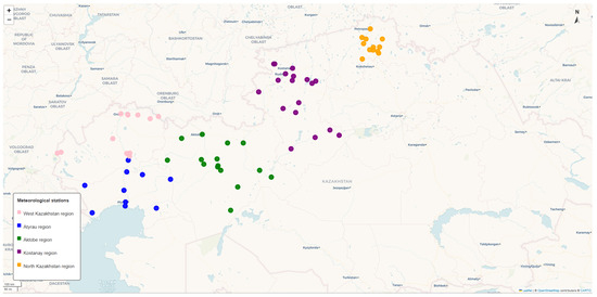
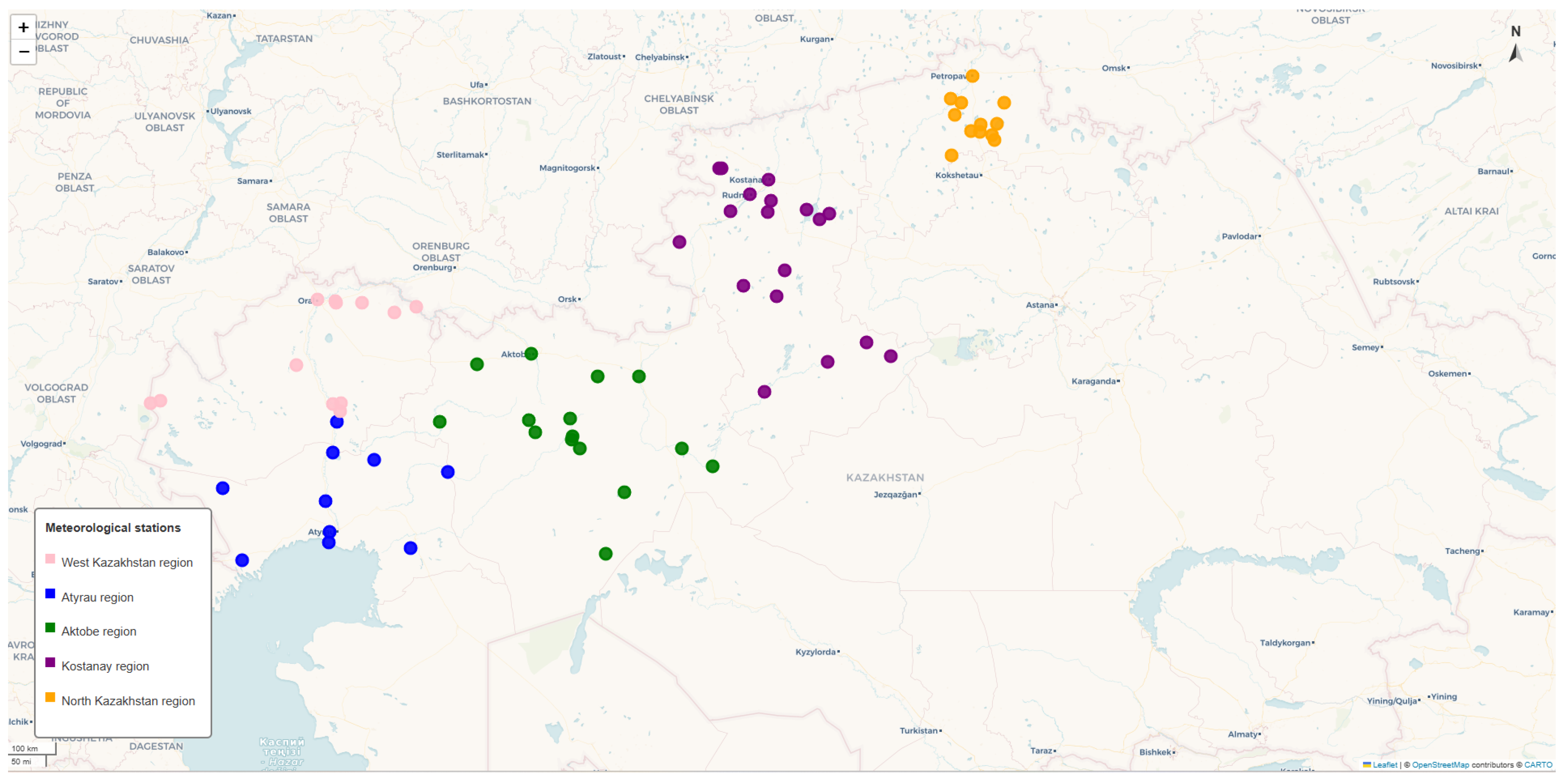
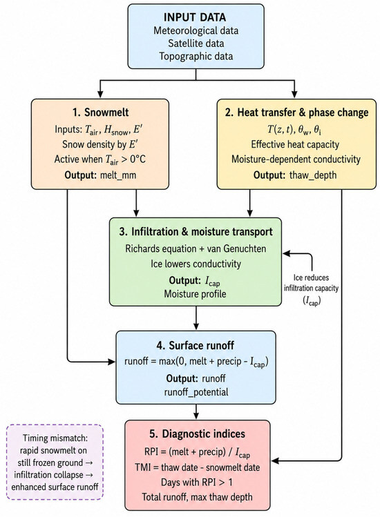
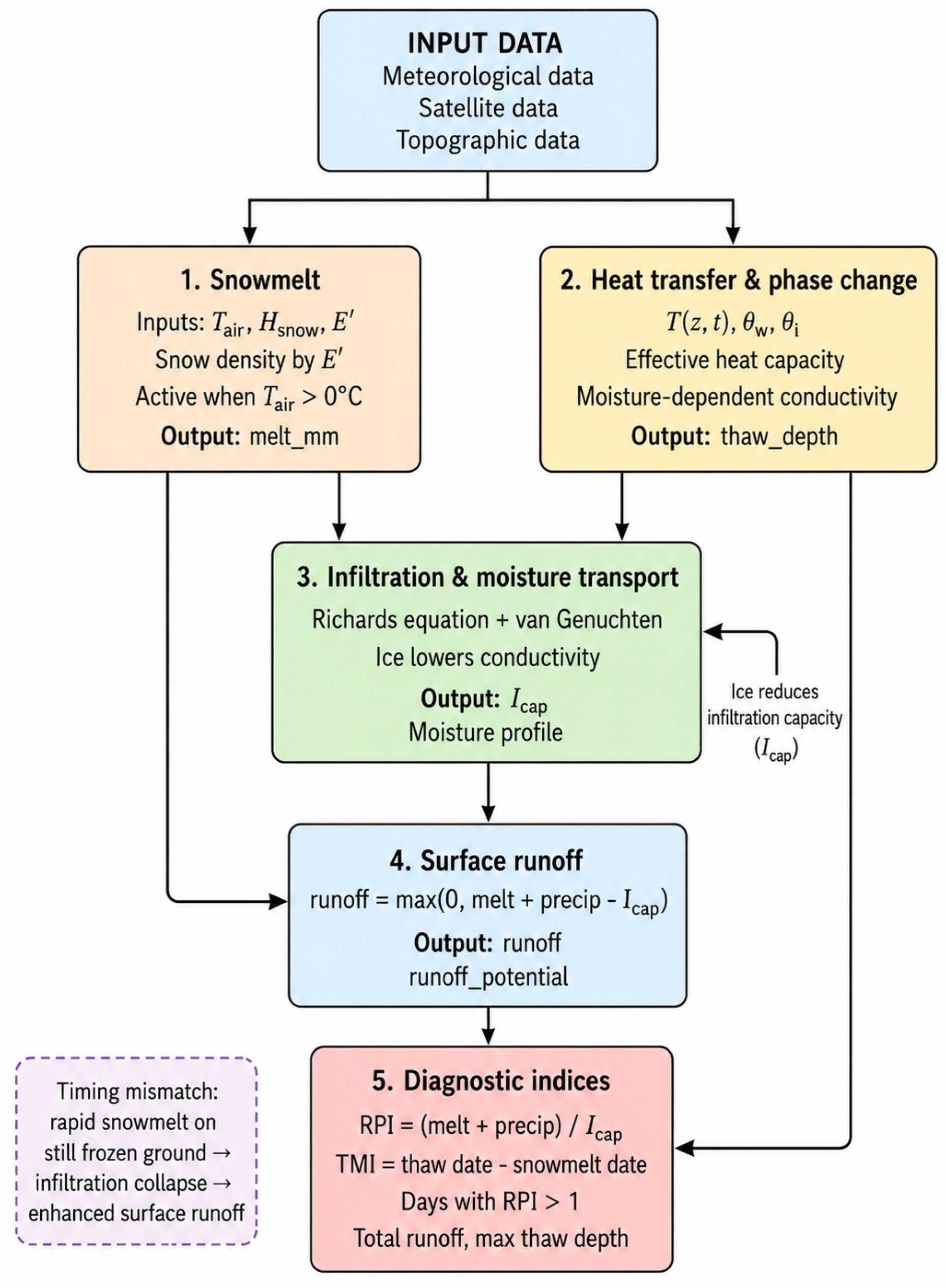
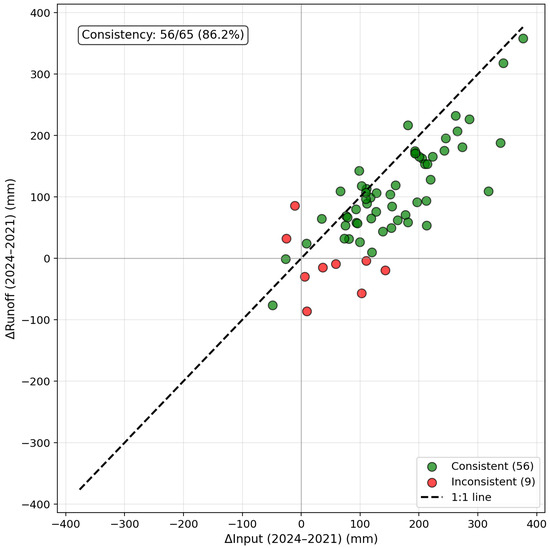
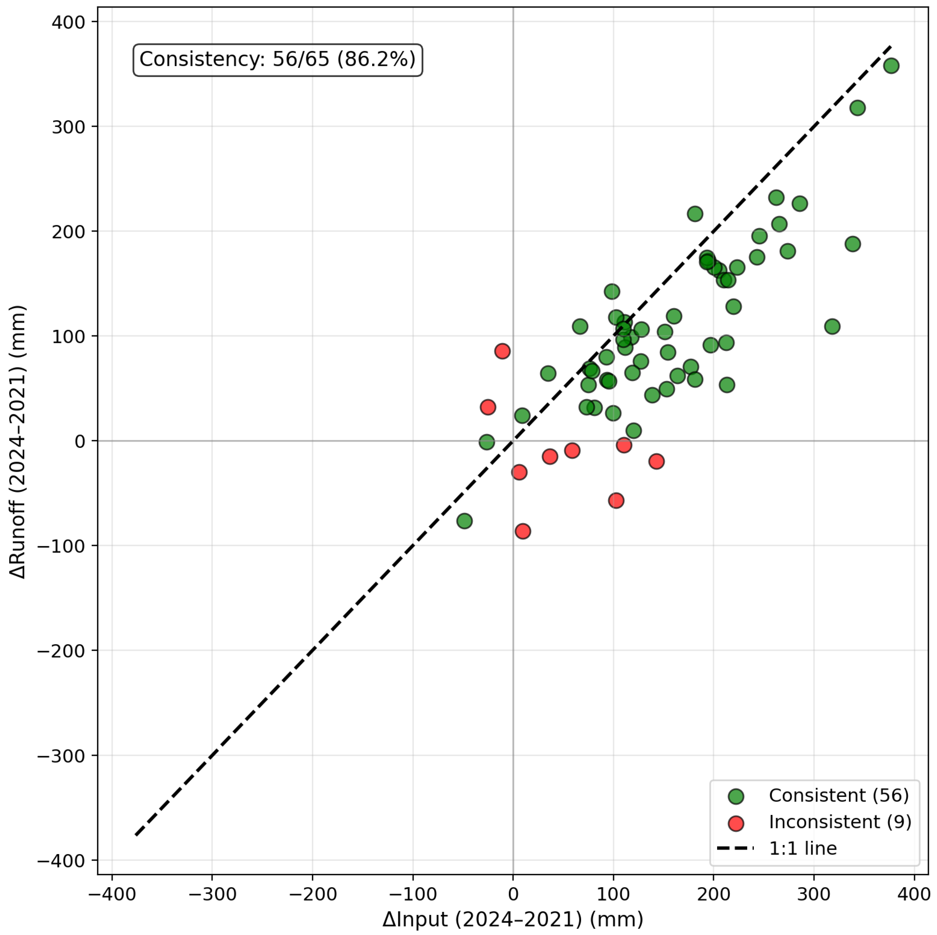
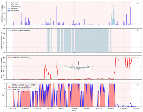
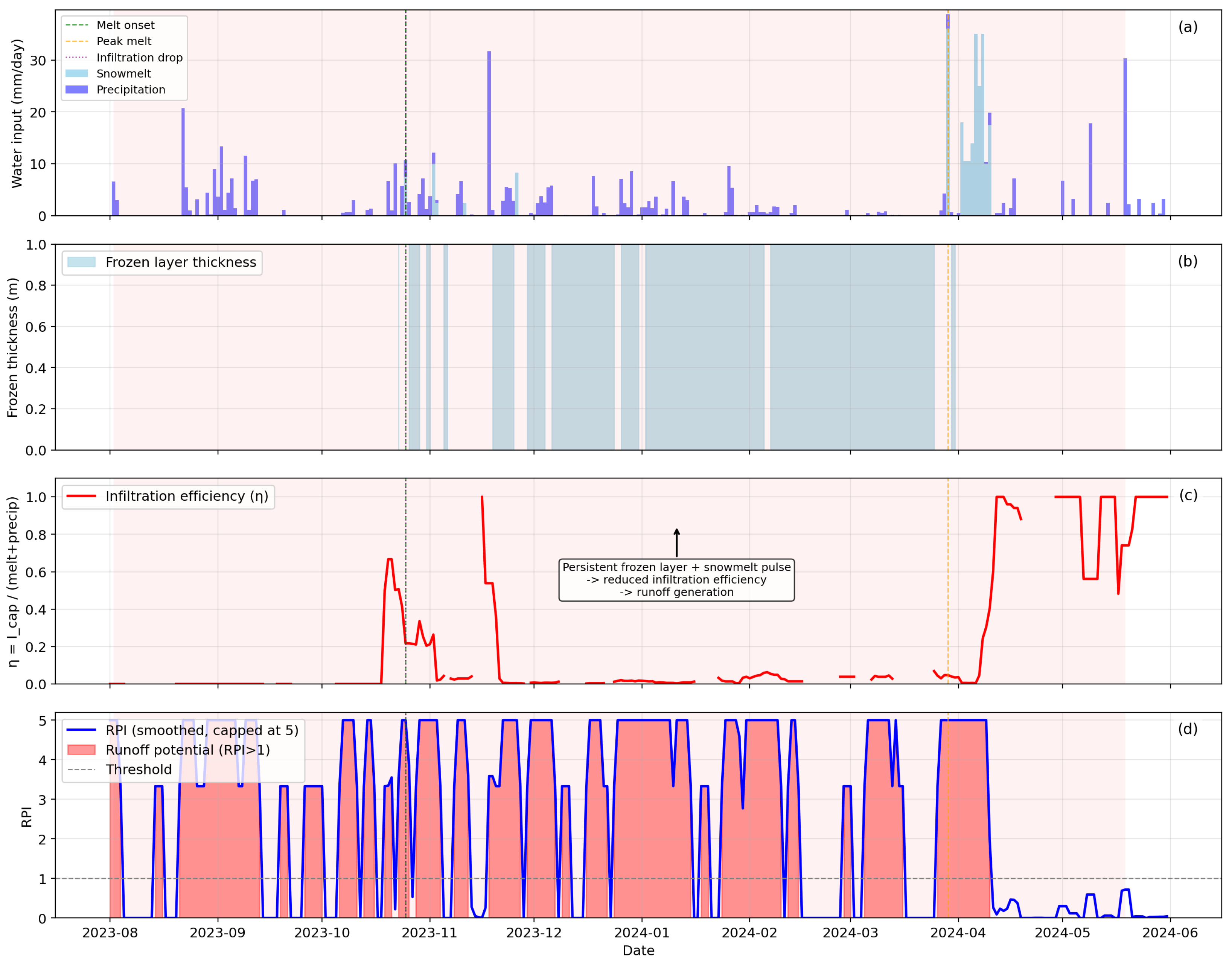
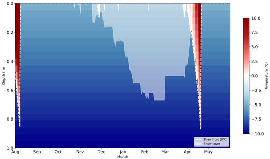
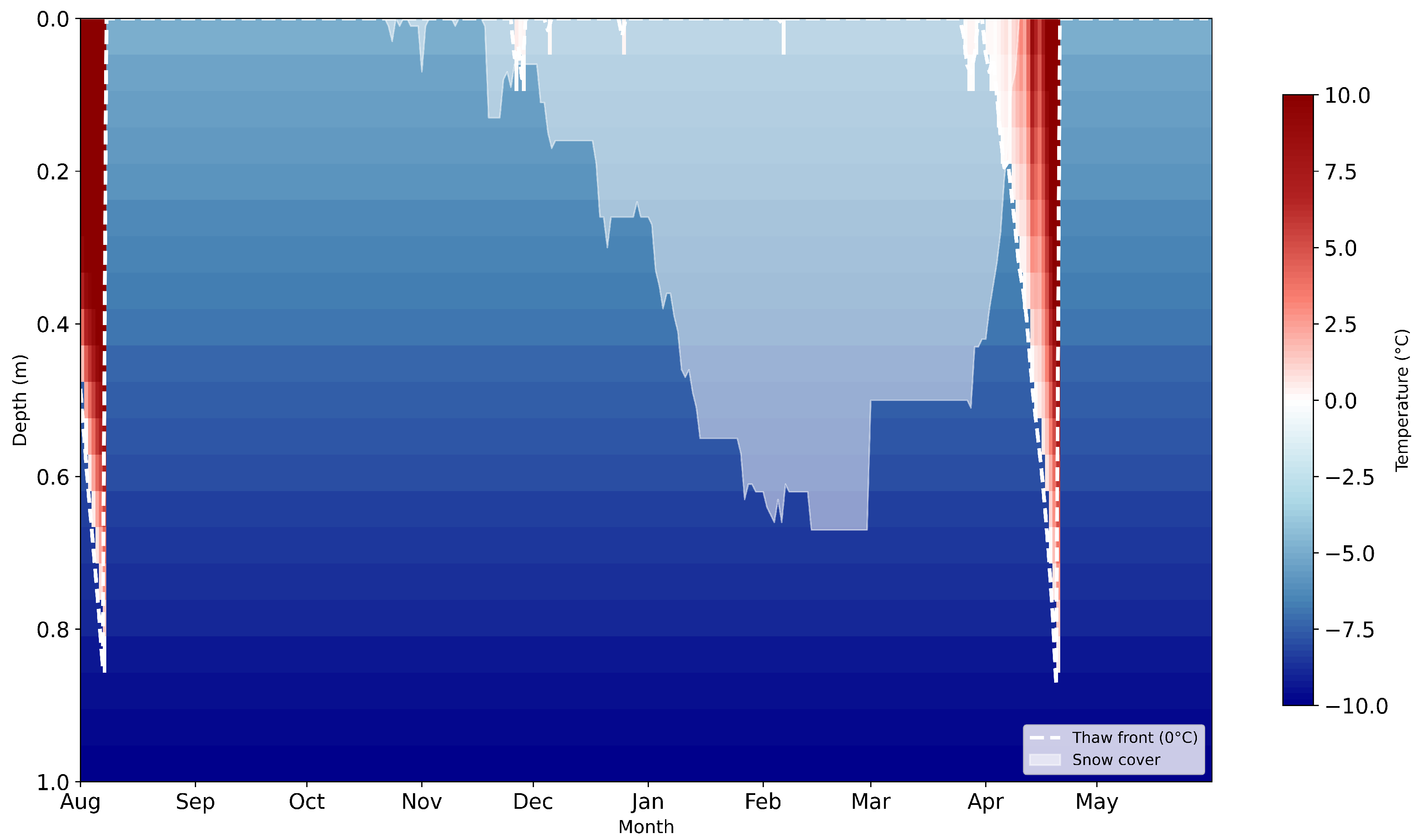
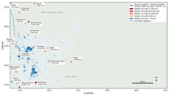
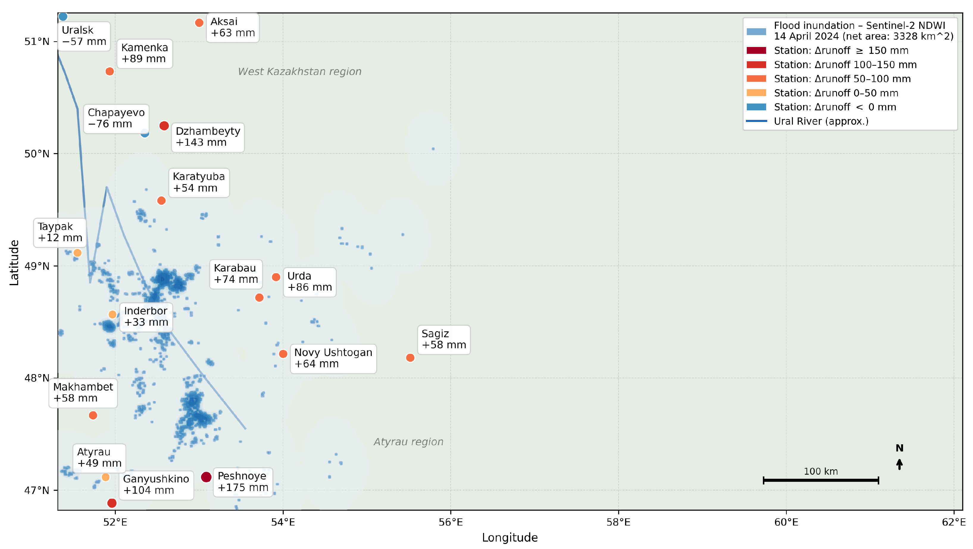

Disclaimer/Publisher’s Note: The statements, opinions and data contained in all publications are solely those of the individual author(s) and contributor(s) and not of MDPI and/or the editor(s). MDPI and/or the editor(s) disclaim responsibility for any injury to people or property resulting from any ideas, methods, instructions or products referred to in the content. |
© 2026 by the authors. Licensee MDPI, Basel, Switzerland. This article is an open access article distributed under the terms and conditions of the Creative Commons Attribution (CC BY) license.