


Abstract
Digital elevation model (DEM) choice can alter stochastic lava-routing results where crater rims, depressions, and narrow channels are represented differently. We compared four source-location tests at Mount Slamet: an interpreted southwest-trending channel, the central crater, the western rim, and the southern crater. The elevation products were a 0.530 m unmanned aerial vehicle (UAV)-derived surface elevation model, Indonesia’s 8.29 m national DEM (DEMNAS), and 30 m Shuttle Radar Topography Mission (SRTM) data. Each DEM–source combination was run four times with 1500 trajectories per replicate. The analysis distinguishes native-grid summaries from common 30 m support and reports visitation-weighted radial reach, trajectory runout, directional concentration, convergence, and termination. The channel test retains a concentrated southwestward distribution on all three products. The other UAV tests remain close to their source cells and have weak directional concentration, so their bearings do not define a clear preferred direction. Regional products generally produce broader and longer distributions, but the response varies among source locations and is not monotonic with cell size. Frequent routing-exception stops and contrasting scales of fixed routing corrections identify unresolved numerical effects. The comparison demonstrates sensitivity to DEM choice under fixed inputs; it does not establish UAV superiority, eruption probability, or validated inundation limits.
1. Introduction
Lava-flow hazard assessment combines assumptions about where and when effusion may occur with simulations of flow propagation over topography. Flow direction can change when lava encounters shallow depressions, channel margins, scarps, or low-relief obstacles, and successive flow units can modify the surface that controls later pathways [1,2,3,4]. Both model formulation and terrain representation therefore influence simulated inundation. Benchmarking and sensitivity studies recommend evaluating numerical assumptions, topographic uncertainty, and grid resolution rather than treating a single model realization as deterministic [5,6,7,8].
Regional and global DEMs are practical for edifice-scale analysis, but their grid spacing may generalize narrow channels and low-relief drainage divides. Structure-from-motion and multi-view stereo (SfM-MVS) photogrammetry from an unmanned aerial vehicle (UAV) can instead provide sub-metre surface models over targeted areas from overlapping images [9,10,11,12]. Applications at Mount St. Helens, Merapi, and Fagradalsfjall demonstrate that repeated photogrammetric surveys can quantify volcanic morphology, volume change, and lava emplacement where field access is difficult [13,14,15].
Fine pixel spacing does not by itself demonstrate high positional accuracy. Camera calibration, image-network geometry, ground control, independent checkpoints, and bundle adjustment govern the accuracy and repeatability of an SfM product [9,11,16]. A defensible comparison must therefore distinguish the spatial detail represented in a UAV-derived surface from independently validated horizontal and vertical accuracy.
Mount Slamet is an active stratovolcano in densely populated Central Java whose summit comprises overlapping craters, sharp rims, local depressions, and southwest-trending upper-flank pathways [17,18,19,20,21,22]. Activity in 2009 and 2014 was concentrated at the summit [17,18]. The combination of complex near-vent morphology and co-located UAV, DEMNAS, and SRTM coverage makes Slamet a useful setting for evaluating sensitivity to DEM-product choice. The tested source locations are controlled routing experiments rather than probabilistic vent forecasts.
Lava-flow models include rapid stochastic routing tools, cellular-automaton and physics-based models, and lobe-emplacement approaches [23,24,25,26]. Q-LavHA samples downslope directions from local topography and uses FLOWGO to impose a thermorheological path-length constraint [27,28,29]. Its raster values are empirical cell-visitation frequencies conditional on the supplied DEM, source, routing parameters, and random seed. A probabilistic hazard map additionally requires probabilities of eruption occurrence, source location, and event magnitude or duration [30,31,32].
This study asks: (1) which summit-scale landforms are represented differently by the UAV, DEMNAS, and SRTM products; (2) how strongly do simulated support, radial reach, and directional concentration vary among products for four fixed summit-source tests; and (3) which differences persist across stochastic replicates, convergence checks, source-cell displacement, common-support evaluation, and termination diagnostics? The novelty is an explicit product-level comparison that exposes both geomorphic and numerical dependencies rather than treating grid spacing as a single causal variable.
2. Geological and Eruptive Setting
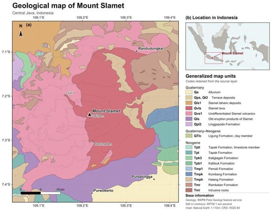
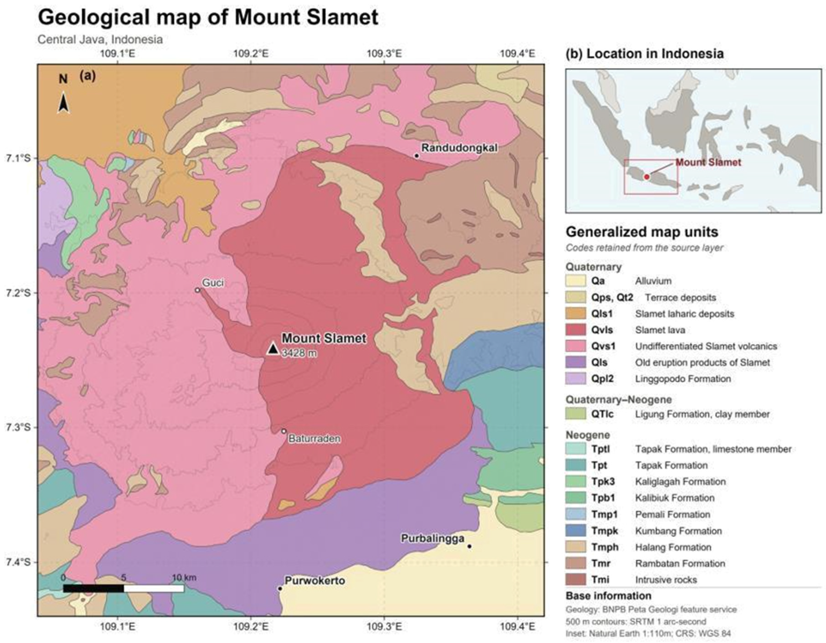
Mount Slamet (3428 m above sea level) lies in the Sunda arc and comprises an older basaltic-andesite to andesite edifice west of a younger basalt to basaltic-andesite summit complex (Figure 1) [18,19,20,21]. Four summit craters and migration of activity toward the southwest, together with scoria cones and lava-bearing units on the flanks, record repeated construction and modification of the edifice [17,18,19,33,34].
Figure 1.
(a) Regional geological setting of Mount Slamet, Central Java, Indonesia. Geological polygons and unit codes are from the Badan Nasional Penanggulangan Bencana (BNPB; Indonesian National Agency for Disaster Countermeasure) geology-map feature service (accessed 5 August 2026). The 500 m elevation contours were derived from SRTM 1 arc-second data; inset (b) uses Natural Earth boundaries. The summit marker follows the Smithsonian Global Volcanism Program location.
Recent activity has been predominantly summit-centred and mildly explosive to mixed explosive–effusive. During April–June 2009 (VEI 1), reports described increased seismicity, inflation, ashfall, lava fountains approximately 100–400 m above the rim, and incandescent ejecta on the western flank [18]. The March–September 2014 episode (VEI 2) included recurrent ash emissions, Strombolian-style incandescent ejecta, and ashfall reported as far as 20 km from the summit [17,18].
3. Materials and Methods
3.1. UAV Survey and Elevation Model
3.1.1. Data Acquisition and Survey Geometry
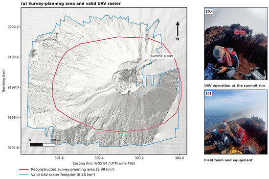
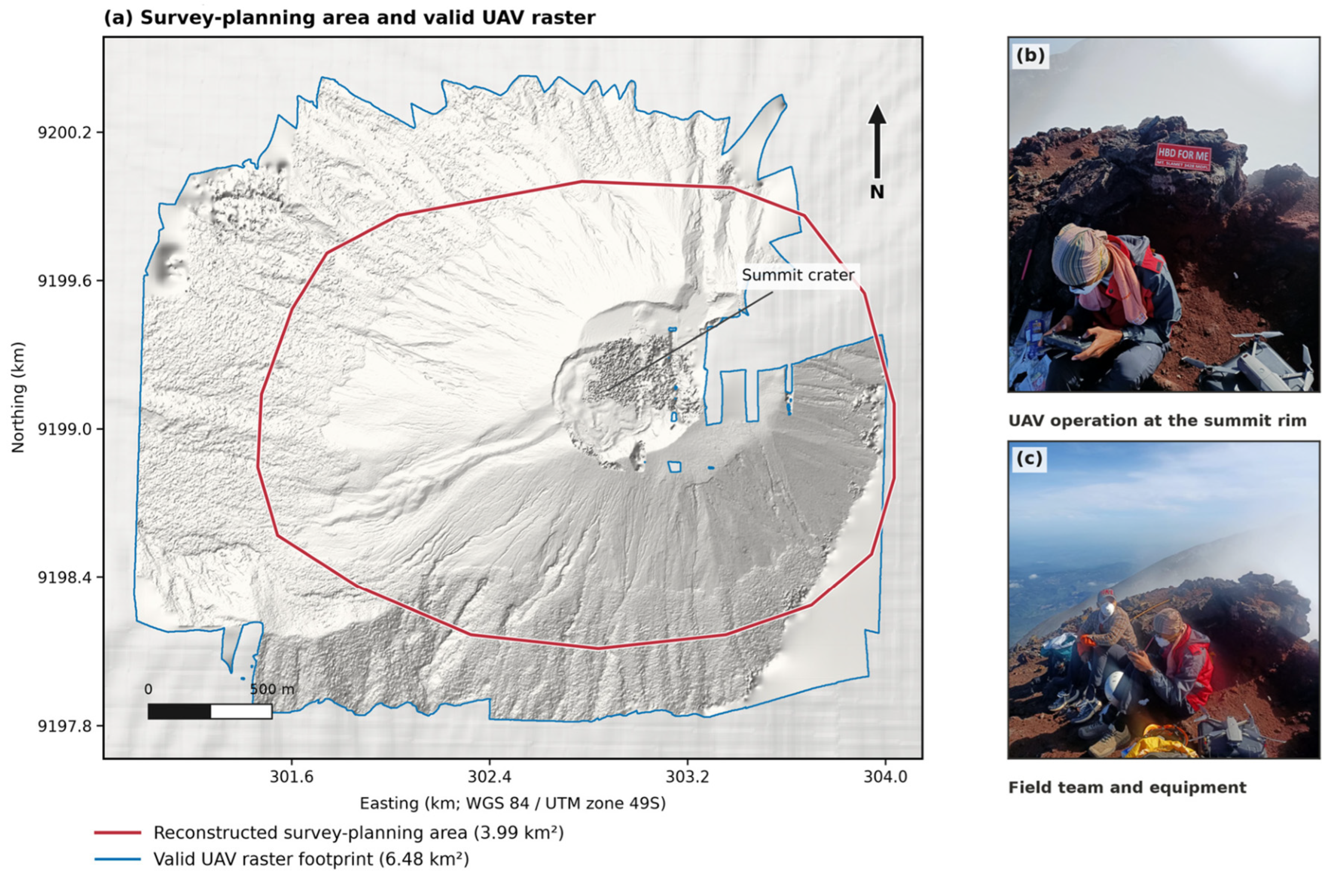
UAV imagery was acquired at the summit on 15 May 2025 with a DJI Mavic 2 Pro (SZ DJI Technology Co., Ltd., Shenzhen, China). Four flight plans combined nadir and oblique views at a nominal height of approximately 200 m above ground, with reported forward and side overlaps of 89% and 75%. The reconstructed survey-planning area is 3.99 km2 (Figure 2). This planning polygon is distinct from both the delivered raster coverage and the valid cells used for simulation. Flight-log tracks were unavailable, so the planning boundary is a cartographic reconstruction rather than a measured GNSS flight path. The rapid summit survey was constrained by steep, unstable crater terrain, limited safe working time, and equipment transport; a surveyed control network was therefore not established.
Figure 2.
UAV survey planning and field acquisition at the Mount Slamet summit. (a) The red boundary outlines the reconstructed 3.99 km2 survey-planning area, and the blue outline identifies the full 6.48 km2 valid-data footprint of the delivered UAV raster. UAV hillshade is displayed within the blue outline, with pale DEMNAS hillshade as regional context. The planning boundary was reconstructed from the supplied map because GNSS flight logs were unavailable; no measured flight tracks are shown. The planning polygon is not the simulation mask, which comprises valid cells within the computational crop described in Section 3.2 and supplied in Supplementary File S1. (b,c) Field operations and equipment on 15 May 2025.
3.1.2. Photogrammetric Processing and Georeferencing
Images were processed in RealityCapture using a structure-from-motion and multi-view-stereo workflow to generate a point cloud, textured surface, orthomosaic, and gridded elevation model [35,36,37]. The archived project does not contain the RealityCapture report, software build, acquired/aligned image counts, camera-calibration export, reconstruction-density setting, or bundle-adjustment diagnostics; unverifiable values are therefore not reported. This missing processing provenance limits exact reconstruction of the photogrammetric workflow. The delivered raster is in WGS 84/UTM zone 49S (EPSG:32749), contains 5862 × 5122 cells at 0.530 m spacing, has 6.48 km2 of valid data within an 8.45 km2 bounding rectangle, and ranges from 2418.0 to 3473.8 m elevation.
Georeferencing relied on the UAV onboard GNSS because the rapid, safety-constrained summit operation did not permit ground-control points (GCPs) or independent checkpoints. Pixel spacing therefore describes spatial sampling, not validated horizontal or vertical accuracy [16]. We use ‘UAV-derived surface elevation model’ or ‘UAV DEM’, not bare-earth DTM, and do not infer centimetre-scale accuracy.
3.2. Comparison with DEMNAS and SRTM
The UAV surface was compared with the Digital Elevation Model Nasional (DEMNAS), Indonesia’s national 0.27 arc-second product (approximately 8.29 m at Slamet), and SRTM 1 arc-second data (approximately 30 m) [38,39]. DEMNAS was bilinearly reprojected to square 8.2895 m cells and SRTM to 30 m cells in EPSG:32749. SRTM HGT values were georeferenced as point posts at their geographic sample coordinates before bilinear reprojection; pixel edges were placed half a sample outside the outer posts. The regional grids covered the UAV bounding rectangle plus a 5 km buffer. To limit memory use, the UAV computational raster was cropped to the envelope of the four source geometries plus 1200 m on each side, clipped to the delivered raster. The UAV crop contains 5.59 km2 of valid cells, distinct from the full delivered coverage of 6.48 km2 and the 3.99 km2 planning polygon. Each simulation retained its product-specific valid-data mask; internal gaps were not filled. Exact input subsets and masks are supplied in Supplementary File S1. No visited footprint contacted an external computational-raster boundary, but this diagnostic does not exclude effects of internal data gaps.
Mapping retained each native grid and used common extents, illumination, and elevation ranges. Vertical references and acquisition epochs were not harmonized. The comparison therefore evaluates complete DEM products, including sampling, alignment, interpolation, surface content, datum, and epoch, rather than resolution in isolation. Non-monotonic results cannot identify which product attribute caused a particular routing difference.
3.3. Q-LavHA Scenarios and Quantitative Metrics
Four controlled source-location tests were evaluated: the interpreted southwest-trending channel, central crater, western rim, and southern crater. The locations sample distinct summit-scale settings visible in the UAV hillshade; they are morphological test sites, not probabilistic vent forecasts. The summit-centred activity described in Section 2 motivates these test locations but does not constrain their exact geometries or probabilities of activation. All simulations used Q-LavHA v3 source package Qlavha_v3_150525 and the FLOWGO terminal-length routine [23,27,32]. The exact implementation, simulation-source SHA-256 hash, and configurations are supplied in Supplementary File S1. Every DEM–source combination was run in four paired-seed replicates of 1500 trajectories (6000 trajectories per ensemble); seeds were 20,260,905 + 100 × scenario index + replicate index.
Q-LavHA samples one of the locally viable neighbours using elevation differences modified by fixed correction heights hc and hp; the 16-neighbour fallback is used if the 8-neighbour window provides no viable continuation. FLOWGO updates channel thermal and rheological state until its stopping criterion is met [23,32]. Inputs are the DEM, source geometry, routing settings, and FLOWGO parameters; outputs are trajectory paths and conditional cell-visitation frequencies. The effusion rate and viscosity are illustrative baseline inputs rather than Mount Slamet calibrations (Table 1).
Table 1.
Q-LavHA configuration, post-processing, and diagnostic settings.
The nominal reference for each source is the arithmetic mean of its four supplied vertices, not an area-weighted polygon centroid. Q-LavHA constructs an axis-aligned bounding box from those vertices. Because each box is narrower and shorter than the 90 m source spacing, the surface-source routine selects only its southwest corner. That coordinate is then assigned to its containing native DEM cell, whose centre is the effective source used in the metrics. The 0.9–44.6 m reference-to-cell distances in Table 2 therefore combine source-position selection within the geometry and raster snapping; they are not snapping distances alone. Supplementary File S1 provides the original vertices, bounding boxes, southwest sampled coordinates, effective cell centres, and the separate displacement components.
Table 2.
Source geometry, nominal reference, and effective source cell by elevation product. Coordinates are metres in WGS 84/UTM zone 49S. The nominal reference is the mean of the four input vertices. Reference-to-cell distance combines southwest-corner selection and raster snapping, as defined in Section 3.3; it is not raster snapping alone. η = hc/(sΔ), where s is a dimensionless local gradient. Elevations are not cross-product accuracy estimates because vertical references were not harmonized.
For native grid i, cell-visitation frequency is pi = ni/N, where ni is the number of trajectories visiting the cell and N = 1500 per replicate. Native A1% is the area of cells with pi ≥ 0.01 and remains a descriptive product-specific metric. We also mapped recorded trajectory positions to a common 30 m evaluation grid. This matches the coarsest simulation grid and gives every counted evaluation cell the same 900 m2 spatial support. Direct comparison of native pixel counts would otherwise confound trajectory visitation with the different native cell areas at 0.530, 8.29, and 30 m spacing. The evaluation grid coincides with the prepared UTM SRTM grid: its upper-left corner is E 295,939.262 m, N 9,205,485.424 m, with 437 columns and 424 rows. Its bounds are E 295,939.262–309,049.262 m and N 9,192,765.424–9,205,485.424 m. It covers the full regional rectangle without an intersection mask shared by the three products. Each recorded native-cell centre was assigned to the containing evaluation cell by floor indexing, and each trajectory counted at most once per evaluation cell. Cells crossed only by a segment between recorded positions were not added. Final visitation-frequency rasters were not interpolated.
The visitation-weighted cumulative radial distribution is Fvis(r) = [Σi pi 1(ri ≤ r)]/[Σi pi] over all non-zero cells; P95vis is the smallest radius containing 95% of visitation weight. Separately, P95traj is the 95th percentile of the maximum radial distances attained by individual trajectories. Directional diagnostics are the source-to-weighted-centroid displacement dc, centroid bearing, and visitation-weighted angular resultant length Rθ (0 = dispersed or compensating directions; 1 = concentrated). Areas, percentiles, dc, and Rθ in Table 3 are arithmetic means of the four replicate statistics, with sample standard deviations where shown. Bearings are circular means of the replicate bearings, obtained from their mean sine and cosine components and wrapped to 0–360° clockwise from north. These summaries are not statistics recalculated from the pooled ensemble. Convergence checkpoints at 250, 500, 1000, and 1500 trajectories were retained for the first replicate of each of the 12 DEM–source combinations, not for all four replicates. Common-grid support was evaluated at p ≥ 0.005, 0.01, and 0.02.
Table 3.
Routing metrics summarized across four replicates. Areas and percentiles are arithmetic means ± 1 sample SD; dc and Rθ are arithmetic replicate means. Bearings are circular means of the four replicate bearings, as defined in Section 3.3. A1% native and A1% common use p ≥ 0.01 on native cells and the common 30 m evaluation grid, respectively. P95vis is the visitation-weighted radial percentile; P95traj is the 95th percentile of individual maximum radial distances; dc is centroid displacement; Rθ is angular concentration. These numerical summaries are not calculated from the pooled 6000-trajectory raster.
The storage-only sparse accumulator retains the original FlowTracker and FLOWGO state transitions and records only visited cells before aggregation. Its 25-path validation limit was imposed by the stock implementation’s full-raster-per-path memory allocation; identical input seeds produced cell-identical output in that test. The implementation and hashes are included in Supplementary File S1. A numerical safeguard supplies a final finite discharge estimate if the stock FLOWGO bisection leaves it unassigned. The safeguard was not triggered by any of the final 72,000 trajectories. The termination audit distinguishes FLOWGO stops from caught Q-LavHA routing exceptions. Exceptions were recorded by message text rather than subtype; blank messages were grouped as FlowException. The archive cannot distinguish internal-NoData effects from other failures of neighbourhood continuation or identify a unique physical cause of stopping.
To diagnose a possible scale interaction, we calculated η = hc/(sΔ), where Δ is native cell spacing and s is a dimensionless rise/run gradient. Orthogonal elevation derivatives were calculated with NumPy gradient using cell spacing in metres, centred finite differences in the window interior, and one-sided differences at its edges. The gradient magnitude was summarized by the median of finite values in a square window extending approximately 150 m in each coordinate direction from the effective source cell. Thus s is neither a slope angle nor a circular-radius average.
4. Results
4.1. UAV Coverage and Terrain Detail
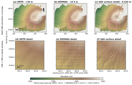
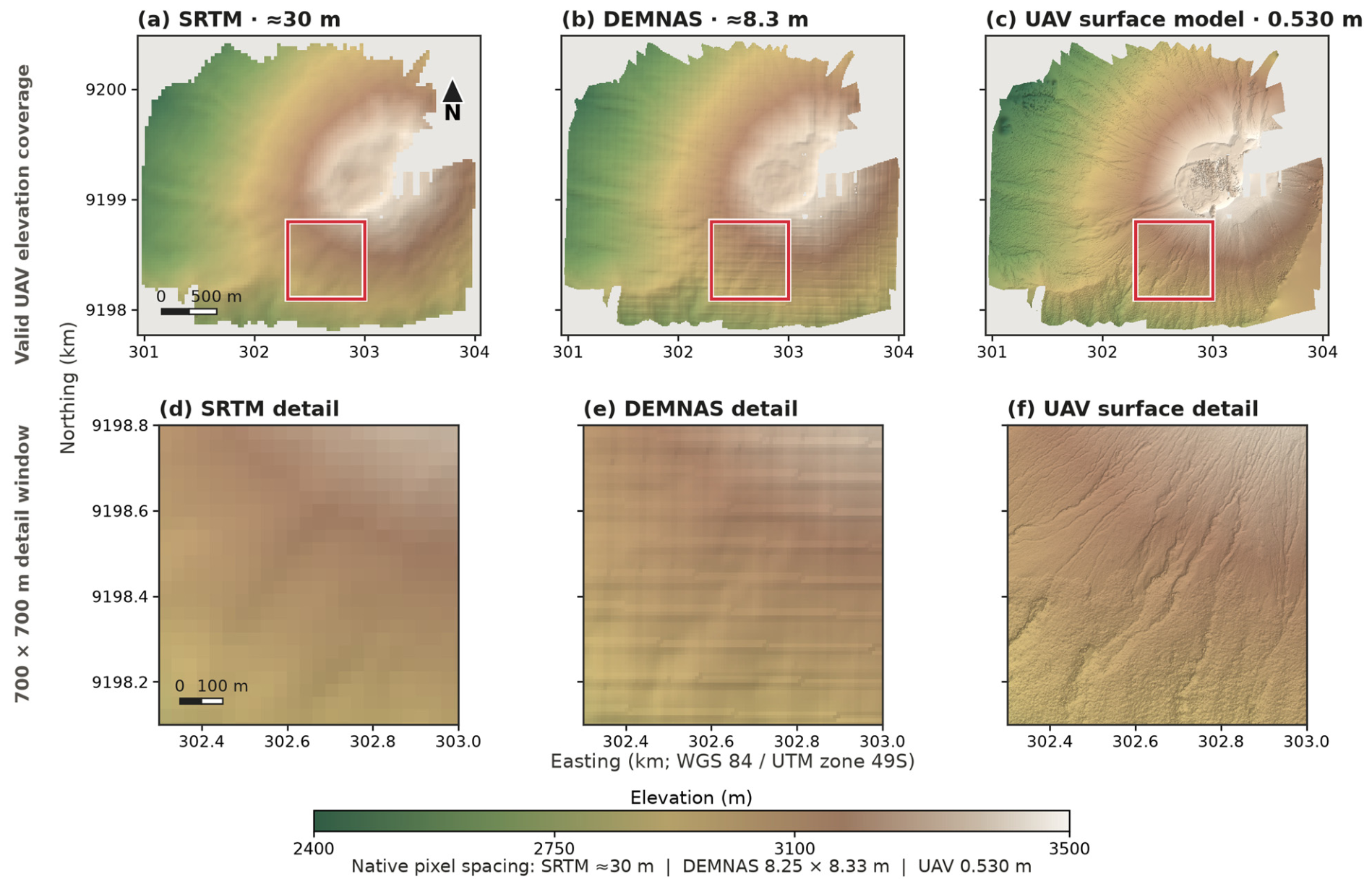
The delivered UAV-derived surface elevation model samples 6.48 km2 of valid summit and upper-flank terrain at sub-metre spacing; internal gaps remain. At the full-map extent, the dominant crater and drainage patterns are visible in all three DEMs. In the 700 m detail window, the UAV hillshade resolves narrow erosional textures and abrupt topographic discontinuities, whereas DEMNAS and SRTM retain broader slope and drainage patterns (Figure 3). The matched cross-sections below examine how those differences affect the representation of a rim, a channel, and a depression sector.
Figure 3.
Comparison of SRTM, DEMNAS, and UAV-derived elevation models. Panels (a–c) show the 6.48 km2 UAV footprint within its 8.45 km2 raster bounding rectangle; panels (d–f) show the same 700 × 700 m window outlined in red. Elevation range, map extent within each row, and illumination are held constant. Native pixel spacing is approximately 30 m for SRTM, 8.29 m for DEMNAS, and 0.530 m for the UAV model. Vertical datums and acquisition epochs were not harmonized, so the figure evaluates spatial detail rather than quantitative elevation differences or vertical accuracy.
4.2. Summit Morphology Interpreted from the UAV DEM
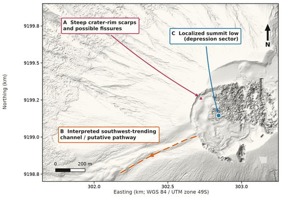
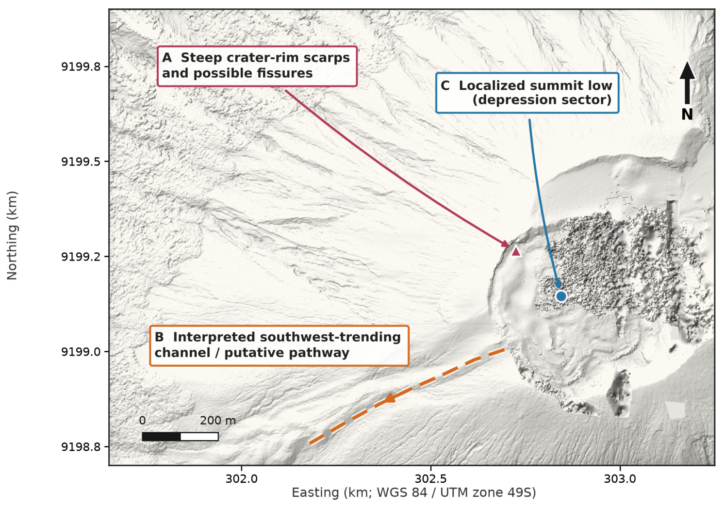
Interpretation of the UAV hillshade identifies: (i) a steep western crater rim with sharp scarps and possible fissure traces; (ii) an interpreted southwest-trending channel extending from the crater margin; and (iii) a localized summit-low sector (Figure 4). These annotations are morphological interpretations rather than independently mapped or dated lava units. The channel is treated as a putative pathway. A low in a cross-section does not establish a closed depression or lava-storage capacity.
Figure 4.
Interpreted morphological features on the UAV hillshade: (A) steep crater-rim scarps and possible fissures, (B) an interpreted southwest-trending channel or putative pathway, and (C) the localized summit-low sector examined by C–C′. Markers identify representative locations, and the dashed line follows the interpreted channel axis. The annotations do not establish fissure origin, a historical lava-flow age, or the closure and storage capacity of the summit low.
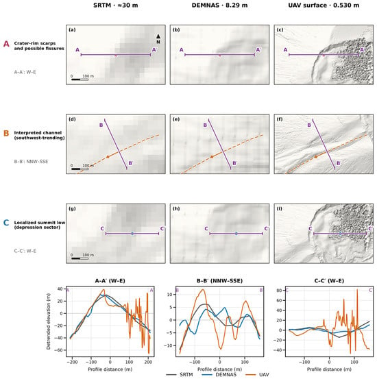
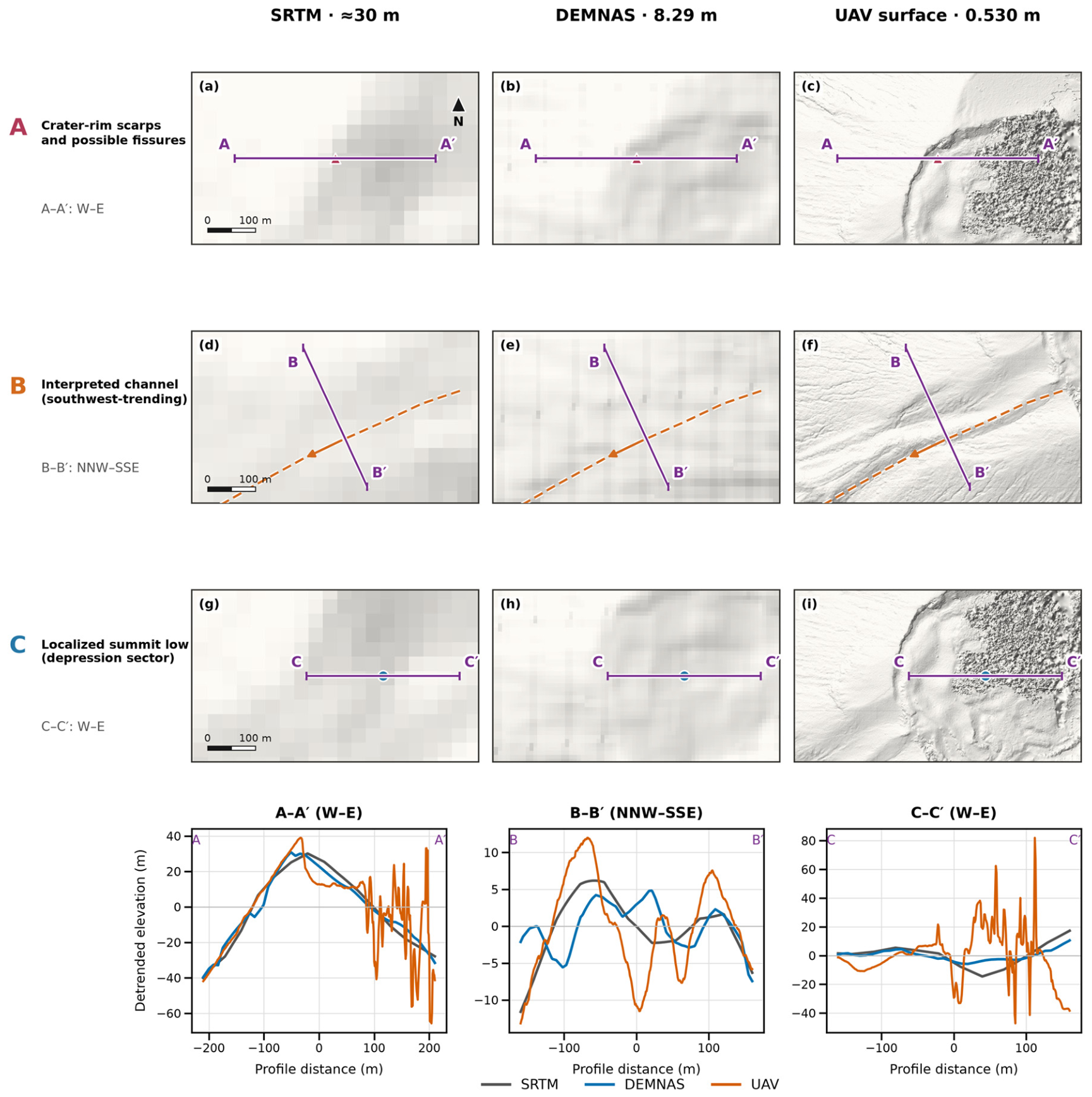
At matched locations, the products differ in both the shape and position of local relief (Figure 5). Profile A–A′ crosses the crater-rim sector. The UAV curve has a sharp local crest and an abrupt drop on its eastern side, while DEMNAS and SRTM represent a broader rim envelope with differently positioned crests. Farther east, the UAV curve contains rapid variations absent from the regional profiles. These are differences in the represented surface, rather than evidence that every short-wavelength feature is real terrain.
Figure 5.
Matched 600 m × 360 m hillshade windows: (a) SRTM, (b) DEMNAS, and (c) UAV in the crater-rim sector; (d) SRTM, (e) DEMNAS, and (f) UAV across the interpreted southwest-trending channel; and (g) SRTM, (h) DEMNAS, and (i) UAV in the summit-low sector. Corresponding lower panels show profiles A–A′, B–B′, and C–C′. Illumination is identical. Purple A–A′, B–B′, and C–C′ traces locate each profile in every corresponding map; the dashed orange line is the interpreted channel axis. Exact endpoints are supplied in Supplementary File S1. Elevations were bilinearly sampled at 1 m intervals and linearly detrended separately for each product. No moving-average smoothing or interpolation across NoData gaps was applied. The plotting interval does not imply 1 m information in the regional DEMs. Profile interpolation is for display and was not applied to the simulation inputs.
Profile B–B′ cuts across the interpreted channel. The UAV curve contains a central trough bounded by higher margins; the regional curves have broader, differently positioned variations and do not reproduce the same trough-and-margin geometry. Relative to a straight chord joining the same profile positions at −68 and +105 m, the maximum represented trough deficit is 21.7 m on the UAV surface, 4.9 m on DEMNAS, and 5.9 m on SRTM. This descriptive measure is relevant to local channel geometry, but it is neither an independently verified channel depth nor a measure of lava thickness or storage capacity.
Profile C–C′ crosses the summit-low sector. The UAV surface contains local lows, intervening highs, and abrupt spikes, whereas the regional curves vary more gradually. The spikes may include photogrammetric reconstruction artefacts; without independent control, their contribution cannot be separated from true surface roughness. Linear detrending removes each product’s overall gradient, and different control, vertical references, and epochs prevent interpreting residual amplitudes as absolute elevation errors. Neither these profiles nor the hillshade establish a closed storage depression or validate individual simulated routes.
Containing-cell sampling at intervals finer than native grid spacing can produce stepped residuals after detrending. Bilinear interpolation was used for the descriptive profiles to avoid this extraction artefact, without moving-average smoothing or interpolation across data gaps. The interpolation does not add native terrain information and was not applied to the simulation DEMs.
4.3. DEM-Product Sensitivity of Simulated Routing
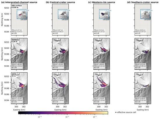
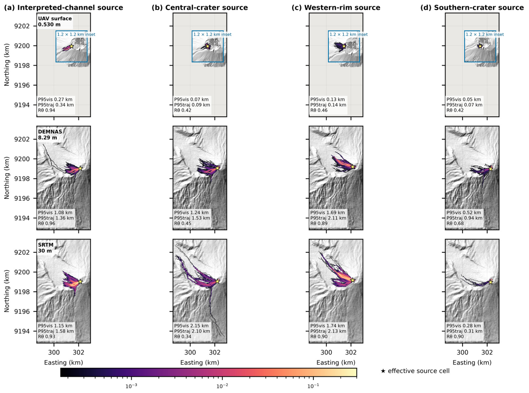
The interpreted-channel test retains a concentrated southwestward distribution on all three elevation products (Table 3; Figure 6). On the UAV surface, trajectories follow a narrow corridor associated with the interpreted trough; DEMNAS and SRTM produce broader and longer distributions in the same general sector. The persistent broad direction is consistent with channel-scale confinement across the three representations. The different reaches cannot be assigned solely to channel geometry because the effective source cells, local grid gradients, and termination behaviour also differ. All reported support areas describe conditional trajectory visitation rather than physical lava inundation.
Figure 6.
Four-replicate Q-LavHA ensembles for the interpreted-channel, central-crater, western-rim, and southern-crater tests on the UAV, DEMNAS, and SRTM surfaces. Map colours show pooled native-grid visitation across 6000 trajectories; the numerical annotations are arithmetic means of the four replicate statistics. All 12 main panels share one extent and scale. Blue-bordered 1.2 × 1.2 km insets reveal compact UAV patterns without changing the main-map comparison. Colours use one logarithmic conditional visitation-frequency scale. Stars mark effective source cells. P95vis, P95traj, and Rθ are defined in Section 3.3. Outputs are sensitivity diagnostics, not eruption probabilities or forecast inundation.
The central-crater test shows the largest contrast in reach. UAV trajectories remain close to the source and spread in partially compensating directions, producing a small centroid displacement and weak angular concentration. DEMNAS and SRTM trajectories extend farther onto the outer slopes, with the longest central distribution on SRTM. However, SRTM has less support above the common-grid 1% threshold than DEMNAS: radial reach and thresholded support area respond differently. The different representations of rim and crater-floor relief provide a plausible geometric context for these routes. The compact UAV pattern cannot establish physical crater retention because numerical stopping and internal gaps remain unresolved.
At the western rim, the UAV footprint is compact and weakly concentrated, whereas the regional products favour the west-northwest sector. DEMNAS and SRTM produce similar western radial reaches, with slightly longer mean reach on SRTM. The regional products therefore agree more closely in the broad western routing pattern than either agrees with the compact UAV distribution.
The southern-crater UAV footprint is similarly compact. DEMNAS and SRTM favour a northerly sector, but the small UAV centroid displacement makes its nominal bearing unsuitable evidence of an opposing dominant direction. DEMNAS gives greater southern radial reach and broader support on the common grid than SRTM, so the DEMNAS–SRTM ordering differs from the central test. Across all tests, P95vis summarizes the radial distribution of visited cells, whereas P95traj is the 95th percentile of the maximum radial distances attained by individual trajectories. They weight the trajectory ensemble differently and should not be treated as interchangeable measures of runout.
The termination audit limits physical interpretation of these contrasts. Most UAV trajectories outside the channel test end with a routing exception, whereas trajectories on DEMNAS and SRTM usually reach the FLOWGO stopping criterion. Short UAV routes are therefore consistent with restricted local continuation, but the archive cannot separate the effects of internal gaps, resolved roughness, and other neighbourhood constraints. The absence of outer-boundary contact does not resolve those internal effects. The contrast in η likewise identifies potential numerical-scale effects without quantifying their contribution to reach.
Between 1000 and 1500 trajectories, first-replicate P95vis changed by at most 4.1% in 11 of the 12 DEM–source combinations. Central SRTM increased from 2013.6 to 2133.6 m, a 6.0% change. Western UAV P95traj decreased from 155.9 to 122.3 m, a 21.5% change, despite a smaller change in P95vis. These checkpoints were not recorded for the other three replicates. Their final variability is reported separately in Table 3; all checkpoints and percentage changes are provided in Supplementary File S1.
5. Discussion
5.1. Research Question 1: Which Terrain Features Differ Among Products?
The UAV product contains sharper local rim transitions and a channel-scale trough than the regional products (Figure 3, Figure 4 and Figure 5), but the abrupt variations in the crater-floor sector may include reconstruction artefacts. Finer sampling does not establish higher absolute accuracy. The absence of GCPs and processing diagnostics prevents ranking elevation fidelity, and the interpreted channel is neither independently mapped nor dated. Its correspondence with a UAV-based route provides geometric context rather than independent validation [1,2,3,4,9,11,16].
Feature generalization can change local connectivity, yet the simulations do not isolate that mechanism. Acquisition epoch, datum, interpolation, grid origin, source snapping, neighbourhood geometry, hc and hp, and NoData configuration also differ or interact among products. The practical result is product-dependent routing; a causal resolution test would aggregate one controlled surface at fixed origin, mask, datum, and source coordinates.
5.2. Research Question 2: How Do the Simulated Distributions Differ?
Native-grid A1% compares different spatial events: visiting part of a 30 m cell is not equivalent to visiting a 0.530 m cell. The common 30 m evaluation grid gives recorded positions equal cell support and still shows broader regional-product support in these tests. It does not equalize native propagation steps, raster masks, or cells crossed between recorded positions. P95vis and P95traj likewise show generally longer regional routes, but neither is a physical inundation area or a calibrated event runout [7,8].
The response is not monotonic across products and metrics. DEMNAS exceeds SRTM in southern reach and common support, while SRTM produces the longest central routes but a smaller central support area above the common-grid 1% threshold. These patterns do not isolate grid alignment or connectivity as their cause. The η diagnostic shows that hc is much larger relative to the local one-cell elevation-drop scale on the UAV grid than on SRTM. This is a potential source of numerical sensitivity, not a measured causal contribution. Controlled synthetic-plane, synthetic-channel, and fixed-path-length experiments would be needed to separate it from terrain representation.
The termination audit further limits physical interpretation. Most non-channel UAV trajectories end with a routing exception, whereas almost all regional trajectories reach the FLOWGO criterion. The logged exceptions do not distinguish internal-NoData effects from other failures of neighbourhood continuation. A compact simulated footprint therefore cannot be treated as evidence that a real lava flow would be trapped at the same location. The tested surfaces and fixed numerical configuration jointly define the conditional routing results.
For operational applications, these issues warrant explicit conditioning and parameter tests. The Q-LavHA user guide recommends filling NoData gaps and abnormal sinks before simulation [27]. Small internal gaps could be interpolated where surrounding observations support the interpolation, and sensitivity to smoothing or sink treatment could be assessed against the original terrain. The correction heights hc and hp should also be tested relative to cell spacing and local relief. Such changes are not automatic improvements: indiscriminate sink filling can remove genuine crater depressions, and smoothing can erase channel margins. Their effects would require separate evaluation; conditioned-DEM simulations were not performed here.
5.3. Research Question 3: Which Contrasts Are Stable?
The interpreted-channel test retains a concentrated southwestward distribution across products. In contrast, the compact UAV central, western, and southern footprints have low Rθ and small dc; their bearings do not define reliable preferred directions. Four-replicate spread remains substantial for western UAV trajectory runout, while the first-replicate central SRTM checkpoints show continuing change in visitation-weighted reach.
Convergence is metric- and scenario-specific rather than guaranteed by 1500 trajectories. Checkpoint histories were retained only for the first replicate and provide a different diagnostic from variability among four completed replicates. The larger late change in western UAV P95traj illustrates why a stable visitation-weighted percentile alone cannot establish runout convergence. The complete checkpoint and replicate tables and the 0.5%, 1%, and 2% support thresholds are supplied in Supplementary File S1.
5.4. Scope, Reproducibility, and Hazard Use
The main limitations are unvalidated UAV georeferencing and incomplete photogrammetric provenance; different product epochs, datums, masks, and alignments; fixed routing and FLOWGO parameters across very different cell sizes; southwest-corner source selection followed by raster snapping; frequent UAV routing-exception stops without causal classification; and no rheological or source-position perturbation ensemble. The sparse accumulator changes storage, while the numerical guard and source code are documented in Supplementary File S1. These constraints preclude forecast or exclusion-zone use [5,6,26,33,34].
A controlled aggregation experiment on a validated, GCP-constrained surface would help separate terrain detail from numerical discretisation. It should retain common masks and grid origins, perturb the source position, and test hc, hp, effusion rate, and rheology on synthetic planes and channels before application to natural topography. Satellite thermal observations can constrain event-specific source and discharge inputs when scene identifiers, bands, calibration, and processing are traceable [28,31,40,41,42,43,44,45,46,47]. The present configuration and outputs are supplied as Supplementary File S1 so that the exploratory comparison can be inspected and reproduced.
6. Conclusions
First, the UAV surface represents sharper local rim and channel relief and more short-wavelength summit variability than DEMNAS and SRTM. Its finer sampling does not establish superior absolute accuracy, and the abrupt summit variations may include reconstruction artefacts. The southwest-trending feature is an interpreted pathway rather than a mapped historical lava channel; the summit-low profile does not establish closed storage geometry.
Second, the tested DEM products produce different conditional trajectory supports and radial-reach distributions under one fixed Q-LavHA/FLOWGO configuration. The interpreted-channel test remains broadly southwestward and concentrated. Bearings from the compact, weakly concentrated UAV footprints at the other source locations do not define reliable preferred directions. Common-support mapping shows that the contrasts persist when recorded positions are evaluated in equal-area cells. The termination and η diagnostics identify unresolved numerical-scale effects and prevent the observed contrasts from being attributed exclusively to terrain representation.
Third, stability depends on the source location and metric. The channel test retains a concentrated southwestward distribution across products and replicates, while western UAV trajectory runout remains variable and central SRTM visitation-weighted reach continues to change between its final checkpoints. Effective source positions, dc and Rθ with bearings, both radial percentiles, common-support frequencies, checkpoint coverage, and termination classifications should be reported explicitly. For Mount Slamet, these outputs support an exploratory sensitivity comparison; they are not eruption probabilities, validated inundation boundaries, or evidence that one DEM is physically superior.
Supplementary Materials
The following supporting information can be downloaded at: https://www.mdpi.com/article/10.3390/geosciences16110447/s1.
Author Contributions
Conceptualization, M.A., D.N. and A.F.S.; methodology, M.A. and A.F.S.; software, M.A. and A.F.S.; validation, D.N., E.K.W. and M.F.R.; formal analysis, M.A., D.N., A.F.S., E.K. and Y.A.P.; interpretation, M.A., D.N., Y.A.P., E.K., E.K.W., R.B.N. and M.H.; expedition and data acquisition, M.A., A.F.S., D.N., M.F.R., M.H., Y.A.P. and E.K.W.; writing—original draft, M.A., D.N., A.F.S. and M.H.; writing—review and editing, A.P., M.A., D.N., E.K.W., R.B.N., Y.A.P., M.H. and A.F.S.; visualization, M.A. and A.F.S.; supervision, D.N.; project administration, D.N.; funding acquisition, D.N. All authors have read and agreed to the published version of the manuscript.
Funding
The research was funded by RIIM BRIN and the Endowment Fund for Education Agency 646 (LPDP) Grants, grant number: AWARD/B1-RIIM-AWARD/18520/1/2024
Data Availability Statement
Supplementary File S1, supplied with this revision as Supplementary_File_S1_Reproducibility.zip, contains the exact Q-LavHA simulation implementation and analysis scripts, version hashes, configuration and seeds, prepared simulation DEM subsets and valid-data masks, source geometries, native and common-grid ensemble rasters, replicate metrics, threshold sensitivity, first-replicate convergence checkpoints, and termination summaries. The archive entry point is README.md. Profile endpoints and extraction details are included with the revised figure scripts. Public DEM provenance and reconstruction information are documented in the archive. The original UAV imagery, RealityCapture processing report, and camera-calibration diagnostics are not included; exact reconstruction of the photogrammetric model is therefore not possible from this archive.
Acknowledgments
The authors thank the Strategic Invitational Research and Innovation for Advancing Indonesia (RIIM) program for supporting this research under contract number AWARD/B1-RIIM-AWARD/18520/1/2024. The authors also acknowledge the field team involved in the Mount Slamet UAV survey.
Conflicts of Interest
The authors declare no conflicts of interest.
References
- Favalli, M.; Mazzarini, F.; Pareschi, M.T.; Boschi, E. Topographic control on lava flow paths at Mount Etna, Italy: Implications for hazard assessment. J. Geophys. Res. Earth Surf. 2009, 114, F01019. [Google Scholar] [CrossRef] [Scilit]
- Favalli, M.; Fornaciai, A.; Mazzarini, F.; Harris, A.J.L.; Neri, M.; Behncke, B.; Pareschi, M.T.; Tarquini, S.; Boschi, E. Evolution of an active lava flow field using a multitemporal lidar acquisition. J. Geophys. Res. Solid Earth 2010, 115, B11203. [Google Scholar] [CrossRef] [Scilit]
- Cashman, K.V.; Soule, S.A.; Mackey, B.H.; Deligne, N.I.; Deardorff, N.D.; Dietterich, H.R. How lava flows: New insights from applications of lidar technologies to lava flow studies. Geosphere 2013, 9, 1664–1680. [Google Scholar] [CrossRef] [Scilit]
- Richardson, P.; Karlstrom, L. The multi-scale influence of topography on lava flow morphology. Bull. Volcanol. 2019, 81, 21. [Google Scholar] [CrossRef] [Scilit]
- Cordonnier, B.; Lev, E.; Garel, F. Benchmarking lava-flow models. Geol. Soc. Lond. Spec. Publ. 2016, 426, 425–445. [Google Scholar] [CrossRef] [Scilit]
- Dietterich, H.R.; Lev, E.; Chen, J.; Richardson, J.A.; Cashman, K.V. Benchmarking computational fluid dynamics models of lava flow simulation for hazard assessment, forecasting, and risk management. J. Appl. Volcanol. 2017, 6, 9. [Google Scholar] [CrossRef] [Scilit]
- Bilotta, G.; Cappello, A.; Hérault, A.; Del Negro, C. Influence of topographic data uncertainties and model resolution on the numerical simulation of lava flows. Environ. Model. Softw. 2019, 112, 1–15. [Google Scholar] [CrossRef] [Scilit]
- Flynn, I.T.W.; Chevrel, M.O.; Crown, D.A.; Ramsey, M.S. The effects of digital elevation model resolution on the PyFLOWGO thermorheological lava flow model. Environ. Model. Softw. 2023, 167, 105768. [Google Scholar] [CrossRef] [Scilit]
- James, M.R.; Robson, S. Straightforward reconstruction of 3D surfaces and topography with a camera: Accuracy and geoscience application. J. Geophys. Res. Earth Surf. 2012, 117, F03017. [Google Scholar] [CrossRef] [Scilit]
- Westoby, M.J.; Brasington, J.; Glasser, N.F.; Hambrey, M.J.; Reynolds, J.M. Structure-from-Motion photogrammetry: A low-cost, effective tool for geoscience applications. Geomorphology 2012, 179, 300–314. [Google Scholar] [CrossRef] [Scilit]
- Smith, M.W.; Carrivick, J.L.; Quincey, D.J. Structure from motion photogrammetry in physical geography. Prog. Phys. Geogr. 2016, 40, 247–275. [Google Scholar] [CrossRef] [Scilit]
- Carrivick, J.L.; Smith, M.W.; Quincey, D.J. Structure from Motion in the Geosciences; Wiley-Blackwell: Hoboken, NJ, USA, 2016. [Google Scholar] [CrossRef] [Scilit]
- Diefenbach, A.K.; Crider, J.G.; Schilling, S.P.; Dzurisin, D. Rapid, low-cost photogrammetry to monitor volcanic eruptions: An example from Mount St. Helens, Washington, USA. Bull. Volcanol. 2012, 74, 579–587. [Google Scholar] [CrossRef] [Scilit]
- Darmawan, H.; Walter, T.R.; Brotopuspito, K.S.; Subandriyo; Nandaka, I.G.M.A. Morphological and structural changes at the Merapi lava dome monitored in 2012–15 using unmanned aerial vehicles (UAVs). J. Volcanol. Geotherm. Res. 2018, 349, 256–267. [Google Scholar] [CrossRef] [Scilit]
- Pedersen, G.B.M.; Belart, J.M.C.; Óskarsson, B.V.; Gudmundsson, M.T.; Gies, N.; Högnadóttir, T.; Hjartardóttir, Á.R.; Pinel, V.; Berthier, E.; Dürig, T.; et al. Volume, effusion rate, and lava transport during the 2021 Fagradalsfjall eruption: Results from near-real-time photogrammetric monitoring. Geophys. Res. Lett. 2022, 49, e2021GL097125. [Google Scholar] [CrossRef] [Scilit]
- James, M.R.; Robson, S.; d’Oleire-Oltmanns, S.; Niethammer, U. Optimising UAV topographic surveys processed with structure-from-motion: Ground control quality, quantity and bundle adjustment. Geomorphology 2017, 280, 51–66. [Google Scholar] [CrossRef] [Scilit]
- Global Volcanism Program. Report on Slamet (Indonesia). Bull. Glob. Volcanism Netw. 2015, 40. [Google Scholar] [CrossRef] [Scilit]
- Global Volcanism Program. Slamet (263180). In Volcanoes of the World; Smithsonian Institution: Washington, DC, USA, 2026; Available online: https://volcano.si.edu/volcano.cfm?vn=263180 (accessed on 5 September 2026).
- Vukadinovic, D.; Sutawidjaja, I.S. Geology, mineralogy and magma evolution of Gunung Slamet volcano, Java, Indonesia. J. Southeast Asian Earth Sci. 1995, 11, 135–164. [Google Scholar] [CrossRef] [Scilit]
- Reubi, O.; Nicholls, I.A.; Kamenetsky, V.S. Early mixing and mingling in the evolution of basaltic magmas: Evidence from phenocryst assemblages, Slamet Volcano, Java, Indonesia. J. Volcanol. Geotherm. Res. 2003, 119, 255–274. [Google Scholar] [CrossRef] [Scilit]
- Harijoko, A.; Sari, S.A.; Wibowo, H.E.; Setiawan, N.I.; Moktikanana, M.L.A. Stratigraphy, chronology, and magma evolution of Holocene volcanic products from Mt. Slamet deposited in the Guci Valley, Central Java, Indonesia. J. Volcanol. Geotherm. Res. 2021, 418, 107341. [Google Scholar] [CrossRef] [Scilit]
- Sutawidjaja, I.S.; Aswin, D.; Sitorus, K. Geologic Map of Slamet Volcano, Central Java, Scale 1:50,000; Volcanological Survey of Indonesia: Bandung, Indonesia, 1985.
- Harris, A.J.L.; Rowland, S.K. FLOWGO: A kinematic thermo-rheological model for lava flowing in a channel. Bull. Volcanol. 2001, 63, 20–44. [Google Scholar] [CrossRef] [Scilit]
- Cappello, A.; Hérault, A.; Bilotta, G.; Ganci, G.; Del Negro, C. MAGFLOW: A physics-based model for the dynamics of lava-flow emplacement. Geol. Soc. Lond. Spec. Publ. 2016, 426, 357–373. [Google Scholar] [CrossRef] [Scilit]
- Tarquini, S.; de’Michieli Vitturi, M.; Jensen, E.H.; Pedersen, G.B.M.; Barsotti, S.; Coppola, D.; Pfeffer, M.A. Modeling lava flow propagation over a flat landscape by using MrLavaLoba: The case of the 2014–2015 eruption at Holuhraun, Iceland. Ann. Geophys. 2019, 62, VO228. [Google Scholar] [CrossRef] [Scilit]
- Pedersen, G.B.M.; Pfeffer, M.A.; Barsotti, S.; Tarquini, S.; de’Michieli Vitturi, M.; Óladóttir, B.A.; Þrastarson, R.H. Lava flow hazard modeling during the 2021 Fagradalsfjall eruption, Iceland: Applications of MrLavaLoba. Nat. Hazards Earth Syst. Sci. 2023, 23, 3147–3168. [Google Scholar] [CrossRef] [Scilit]
- Mossoux, S.; Kervyn, M. Q-LavHA Version 3 User Guide; Centre d’Étude des Risques et Changement Climatique, 2020. Available online: https://cerg-c.github.io/files/Usersguide_Q-LavHA_V3_2020.pdf (accessed on 29 September 2026).
- Ganci, G.; Vicari, A.; Cappello, A.; Del Negro, C. An emergent strategy for volcano hazard assessment: From thermal satellite monitoring to lava flow modeling. Remote Sens. Environ. 2012, 119, 197–207. [Google Scholar] [CrossRef] [Scilit]
- Favalli, M.; Pareschi, M.T.; Neri, A.; Isola, I. Forecasting lava flow paths by a stochastic approach. Geophys. Res. Lett. 2005, 32, L03305. [Google Scholar] [CrossRef] [Scilit]
- Favalli, M.; Tarquini, S.; Fornaciai, A. DOWNFLOW code and lidar technology for lava flow analysis and hazard assessment at Mount Etna. Ann. Geophys. 2011, 54, 552–566. [Google Scholar] [CrossRef] [Scilit]
- Wright, R.; Garbeil, H.; Harris, A.J.L. Using infrared satellite data to drive a thermo-rheological/stochastic lava flow emplacement model: A method for near-real-time volcanic hazard assessment. Geophys. Res. Lett. 2008, 35, L19307. [Google Scholar] [CrossRef] [Scilit]
- Mossoux, S.; Saey, M.; Bartolini, S.; Poppe, S.; Canters, F.; Kervyn, M. Q-LAVHA: A flexible GIS plugin to simulate lava flows. Comput. Geosci. 2016, 97, 98–109. [Google Scholar] [CrossRef] [Scilit]
- Del Negro, C.; Cappello, A.; Neri, M.; Bilotta, G.; Hérault, A.; Ganci, G. Lava flow hazards at Mount Etna: Constraints imposed by eruptive history and numerical simulations. Sci. Rep. 2013, 3, 3493. [Google Scholar] [CrossRef] [Scilit] [PubMed]
- Ogburn, S.E.; Charlton, D.; Norgaard, D.; Wright, H.M.; Calder, E.S.; Lindsay, J.; Ewert, J.; Takarada, S.; Tajima, Y. The Volcanic Hazard Maps Database: An initiative of the IAVCEI Commission on Volcanic Hazards and Risk. J. Appl. Volcanol. 2023, 12, 2. [Google Scholar] [CrossRef] [Scilit]
- Turner, D.; Lucieer, A.; Watson, C. An automated technique for generating georectified mosaics from ultrahigh-resolution UAV imagery, based on structure from motion. Remote Sens. 2012, 4, 1392–1410. [Google Scholar] [CrossRef] [Scilit]
- Seitz, S.M.; Curless, B.; Diebel, J.; Scharstein, D.; Szeliski, R. A comparison and evaluation of multi-view stereo reconstruction algorithms. In Proceedings of the 2006 IEEE Computer Society Conference on Computer Vision and Pattern Recognition, New York, NY, USA, 17–22 June 2006; Volume 1, pp. 519–528. [Google Scholar] [CrossRef] [Scilit]
- Furukawa, Y.; Hernández, C. Multi-view stereo: A tutorial. Found. Trends Comput. Graph. Vis. 2015, 9, 1–148. [Google Scholar] [CrossRef] [Scilit]
- Badan Informasi Geospasial. DEMNAS—Digital Elevation Model Nasional (0.27 Arc-Second; EGM2008) [Data Set], 2018. Available online: https://www.big.go.id/en/content/product/demnas (accessed on 5 September 2026).
- Farr, T.G.; Rosen, P.A.; Caro, E.; Crippen, R.; Duren, R.; Hensley, S.; Kobrick, M.; Paller, M.; Rodriguez, E.; Roth, L.; et al. The Shuttle Radar Topography Mission. Rev. Geophys. 2007, 45, RG2004. [Google Scholar] [CrossRef] [Scilit]
- Francis, P.; Rothery, D. Remote sensing of active volcanoes. Annu. Rev. Earth Planet. Sci. 2000, 28, 81–106. [Google Scholar] [CrossRef] [Scilit]
- Irons, J.R.; Dwyer, J.L.; Barsi, J.A. The next Landsat satellite: The Landsat Data Continuity Mission. Remote Sens. Environ. 2012, 122, 11–21. [Google Scholar] [CrossRef] [Scilit]
- Harris, A.J.L.; Rowland, S.K. Effusion rate controls on lava flow length and the role of heat loss: A review. In Studies in Volcanology: The Legacy of George Walker; Thordarson, T., Self, S., Larsen, G., Rowland, S.K., Höskuldsson, Á., Eds.; Special Publications of IAVCEI; Geological Society of London: London, UK, 2009; Volume 2, pp. 33–51. [Google Scholar]
- Ramsey, M.S.; Harris, A.J.L. Volcanology 2020: How will thermal remote sensing of volcanic surface activity evolve over the next decade? J. Volcanol. Geotherm. Res. 2013, 249, 217–233. [Google Scholar] [CrossRef] [Scilit]
- Coppola, D.; Laiolo, M.; Piscopo, D.; Cigolini, C. Rheological control on the radiant density of active lava flows and domes. J. Volcanol. Geotherm. Res. 2013, 249, 39–48. [Google Scholar] [CrossRef] [Scilit]
- Ramsey, M.S.; Flynn, I.T.W. The spatial and spectral resolution of ASTER infrared image data: A paradigm shift in volcanological remote sensing. Remote Sens. 2020, 12, 738. [Google Scholar] [CrossRef] [Scilit]
- Wright, R.; Flynn, L.P.; Garbeil, H.; Harris, A.J.L.; Pilger, E. MODVOLC: Near-real-time thermal monitoring of global volcanism. J. Volcanol. Geotherm. Res. 2004, 135, 29–49. [Google Scholar] [CrossRef] [Scilit]
- Coppola, D.; Laiolo, M.; Cigolini, C.; Massimetti, F.; Delle Donne, D.; Ripepe, M.; Arias, H.; Barsotti, S.; Bucarey Parra, C.; Centeno, R.G.; et al. Thermal remote sensing for global volcano monitoring: Experiences from the MIROVA system. Front. Earth Sci. 2020, 7, 362. [Google Scholar] [CrossRef] [Scilit]

Disclaimer/Publisher’s Note: The statements, opinions and data contained in all publications are solely those of the individual author(s) and contributor(s) and not of MDPI and/or the editor(s). MDPI and/or the editor(s) disclaim responsibility for any injury to people or property resulting from any ideas, methods, instructions or products referred to in the content. |
© 2026 by the authors. Licensee MDPI, Basel, Switzerland. This article is an open access article distributed under the terms and conditions of the Creative Commons Attribution (CC BY) license.