


Abstract
Shallow supra-salt oils in the Precaspian Basin change with depth, but the controls are rarely tested. This study aims to quantify the vertical contrast in oil properties at Uytas on the south-eastern basin margin, separate its thermal and compositional parts, and identify what controls the formation waters, using ten oil and fifteen water analyses from twelve wells. The 24.0–28.0 °API oils are medium-gravity crudes, viscous in place because the reservoirs are cold. Estimated dead-oil viscosity at reservoir temperature is 234–764 mPa·s in the Lower Cretaceous and 83–112 mPa·s in the Jurassic, with no overlap in density, viscosity, saturates or aromatics (exact permutation p = 0.0048–0.0095). At a common 20 °C the 4.52-fold contrast falls to 2.40, so it is partly thermal. Only salinity separates the waters (7.4–31.4 against 46.1–94.9 g L−1), consistent with recharge in the Cretaceous and dissolved halite in the Jurassic. Regional evidence points to one oil family from sub-salt Palaeozoic source rocks; the remaining contrast is consistent with mild alteration of the shallow oils, which molecular and isotopic analyses can distinguish from multi-stage charge. Needing only routine appraisal data, the approach suits supra-salt fields across the Precaspian Basin and small fluid datasets in other salt basins.
1. Introduction
Salt tectonics creates two petroleum systems in one basin. Below the salt, source rocks are insulated and their maturation is retarded; above it, thin Mesozoic and Cenozoic sequences are broken into small fault blocks by diapir growth and crestal collapse, and hydrocarbons that reach them arrive in traps only a few hundred metres deep [1,2,3,4]. The depositional and structural framework of a basin, which distributes its reservoirs and source rocks, is a first-order control on its petroleum systems, as shown for the late Sinian to early Cambrian intraplatform basin of the Sichuan Basin [5]. The Precaspian Basin, with more than 1500 salt domes [6], contains one of the largest salt-tectonic provinces on Earth, and its supra-salt play has been productive for more than a century; yet, the literature is dominated by the sub-salt carbonate giants [7,8,9]. The supra-salt succession itself has only recently been described systematically at the basin scale [10], the post-salt trapping mechanisms of the south-eastern basin margin have been set out [11], and the accumulations of the Emba region, which are numerous, shallow and cold, are documented mostly in unpublished evaluation reports.
Those accumulations share a fluid problem. Oil in shallow supra-salt traps is commonly viscous, and viscosity varies with depth within a single structure by factors that matter for development: a 400 mPa·s oil and a 100 mPa·s oil in the same structure are different development problems, requiring different well designs, different lift, and in some cases thermal recovery in one interval and cold production in the other [12,13]. Predicting which interval will produce which fluid is therefore a practical question as well as an academic one.
The mechanisms that produce such variation are individually well understood. In-reservoir biodegradation preferentially removes saturated hydrocarbons and raises density, viscosity, sulfur level and the polar fraction [14,15,16,17]. Its rate is limited by temperature, by the supply of nutrients and electron acceptors, and by the area of the oil–water contact rather than by the volume of oil [17,18]. Above roughly 80 °C the reservoir is sterilised, and if a basin is later uplifted the oil remains undegraded even when it returns to temperatures at which degradation would otherwise proceed [19]. High salinity slows degradation independently of temperature [20,21]. Water washing removes the more soluble aromatic compounds and can reproduce part of the same compositional shift [22].
Distinguishing these mechanisms from one another normally requires molecular data. Biodegradation is diagnosed from the depletion of n-alkanes, the growth of an unresolved complex mixture, and the appearance of 25-norhopanes and other demethylated biomarkers [23,24]. Where those data are absent, the same bulk pattern of low saturates, high polars and high sulfur can be produced by a different source facies, a different charge history, or water washing [22,25], and separating alteration from the mixing of charges of different origin requires molecular and isotopic evidence together [26]. What a bulk dataset can and cannot establish in that situation is the question this paper addresses.
Salt adds two complications specific to this setting. Halite conducts heat two to four times better than the clastics around it, so a salt structure focuses heat and, in purely conductive models, raises temperatures in the overburden above its crest while depressing them beneath the salt and adjacent to its flanks [27,28,29,30,31,32,33]. The sign and the magnitude depend on the geometry of the body, on the conductivity contrast, and on whether fluid flow contributes to heat transport, so the effect cannot be assumed from the presence of salt alone [33]. Salt dissolution can also drive density-contrasted groundwater flow that flushes the shallow section [34,35]. Both processes act in the same depth interval as the fluid variation they might be invoked to explain.
A statistical difficulty accompanies datasets of this size. A correlation computed across two stratigraphic groups measures the separation between the groups and can differ in sign from the relation within either of them [36], and samples repeated within one pool make the number of independent units smaller than the number of samples.
This paper takes a single supra-salt field for which a full set of routine appraisal analyses of oil and water is available and asks how much of the fluid variation such a dataset can explain. It quantifies the vertical contrast in oil properties at Uytas, separates the part that is a temperature effect from the part that is a property of the oil, tests the correlations within as well as across the stratigraphic groups, and identifies what controls the formation waters. Each step uses only data that appraisal programmes routinely collect, so the procedure, summarised in Section 5.7, applies directly to other supra-salt fields.
2. Geological Setting
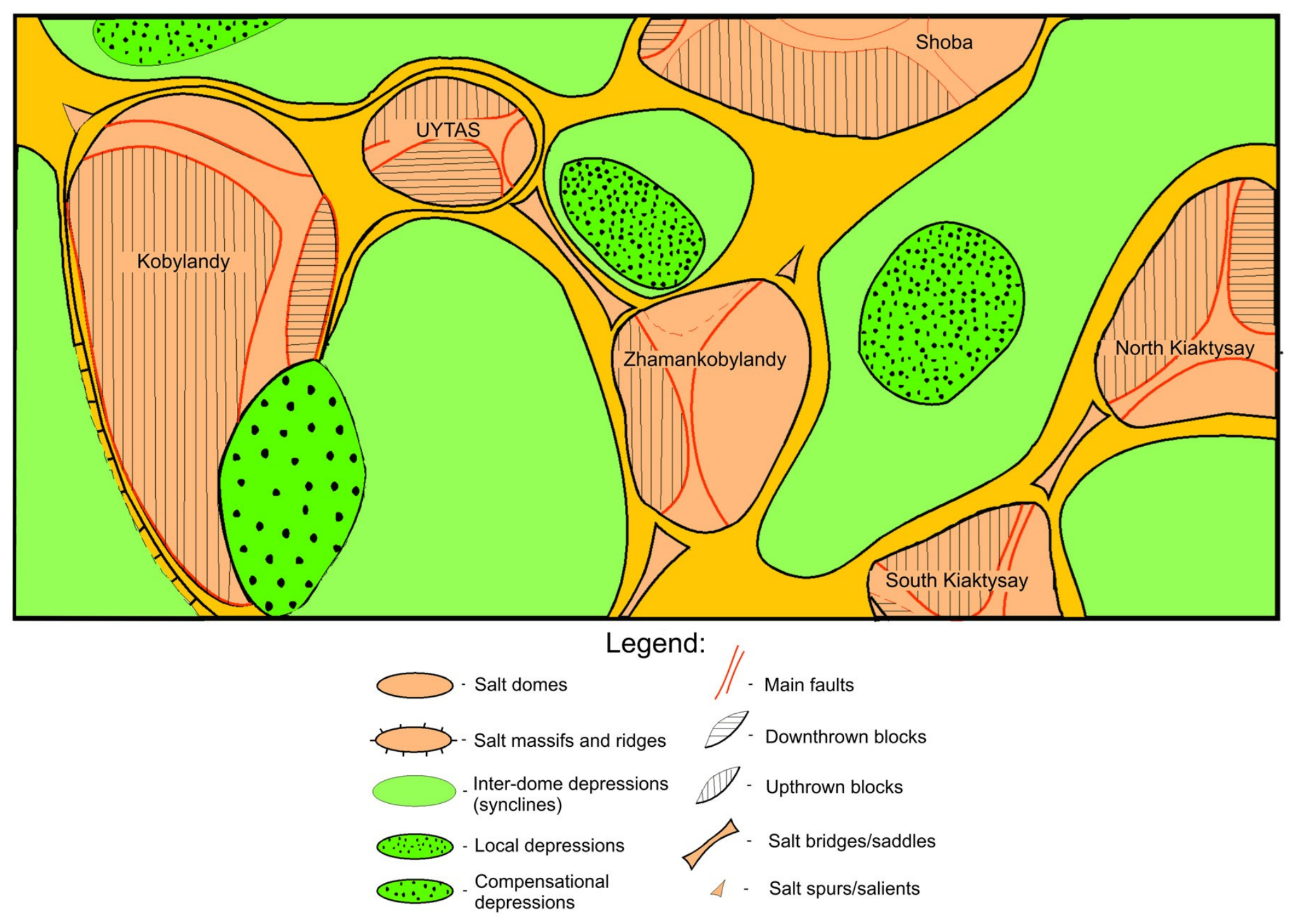
Uytas lies in the Kyzylkoga District of Atyrau Region, Kazakhstan, in the inner marginal zone of the south-eastern Precaspian Basin, within international map sheet L-40 (Figure 1). The field is one of a chain of salt-cored structures that includes Kobylandy, Zhamankobylandy, Shoba and the Kiaktysay structures, separated by inter-dome synclines and connected by salt saddles (Figure 2). Figure 2 shows the salt-tectonic setting of the traps [6,11]; the geometry of the salt beneath the reservoirs underlies the thermal argument of Section 5.5 and the halite contribution to the waters (Section 5.3). Kazakh place names follow the transliteration of the field documentation; their spelling varies between sources [37].
Figure 1.
Location of the study area. (a) Position of the Caspian Sea (blue) and of the area of panel (b) (red frame) on the globe; the dot marks the Uytas structure. (b) Geological sketch map of the North Caspian (Precaspian) Basin and adjacent territories, modified after [10]; the background colours show the surface geology of [10]. Legend: 1—contours of the North Caspian Basin; 2—contours of the main structural elements; 3—A-H: Astrakhan–Aktobe system of uplifts, T-S: Tugarakchan sag, E-E: eastern edge zone, N-E: northern edge zone; 4—C-D: Central Caspian depression; 5—letter designations of allocated zones; 6—settlements; 7—rivers; 8—state border of the Republic of Kazakhstan; 9—licence area; and 10—Uytas structure. Items 9 and 10 are added in this study.
The salt body has a plateau-shaped crest mapped at −380 m and three flanks. On the southern flank, which carries the productive part of the field, the top of the salt falls from the crest to −680 m, then flattens and is traced to −820 m before descending into the adjacent minibasin; a low-amplitude rise on that flat-lying part of the salt surface, matched by a rise in the supra-salt cover, may be structural or an artefact of lateral velocity variation in the depth conversion (Section 3.2). On the northern flank the salt is traced to −760 m; these elevations do not imply dips, because Figure 3c has no true horizontal scale. The eastern flank lies outside the 3D surveys (Section 3.2).
Above the salt, Jurassic and Lower Cretaceous clastics deposited during halokinesis, in the way described for the Permo-Triassic clastics of the nearby Saigak field [38], are cut by normal faults into three limbs. The southern limb is the best constrained and contains all the pools discussed here. Its structure is inherited upward and grows as it does so: at the base of the Jurassic (Horizon V) the closure is contoured at −630 m and measures 2.4 × 1.4 km with an amplitude of 60 m; at the intermediate mapped horizon (Horizon III) it is 3.0 × 1.5 km with an amplitude of 40 m; at the Lower Cretaceous marker it is 3.2 × 1.6 km with an amplitude of 50 m (Figure 3b). These dimensions and amplitudes are approximate values (Section 3.2). The crest migrates west and then south between these levels. A sub-meridional fault with a throw of 20–30 m divides the closure into a western block I and an eastern block II; lower-order faults divide block I into four sub-blocks (Figure 3a) and separate off sub-block IIb, which holds the sampled J-IIB pool, within block II (Table A1).
Cretaceous rocks crop out at the surface over the dome, so the shallow reservoirs subcrop directly beneath Quaternary cover, which provides a potential recharge path into the shallowest pools. Seismic sections through well UTS-1 show the Cretaceous, Jurassic and Permo-Triassic sequences resting on the Kungurian salt and the fault pattern that breaks them (Figure 4).
Figure 2.
Schematic salt-tectonic framework of the Uytas area, not to horizontal scale: salt domes and massifs, the saddles and ridges connecting them, the local depressions and the inter-dome synclines; Uytas is labelled at the top. Simplified by the authors after the summary structural maps of the supra-salt deposits and the top of the salt in [39]; the eastern flank of the Uytas salt body and the salt periphery, including the saddles, lie outside the 3D surveys (Section 3.2). The regional setting is described in [6,11].
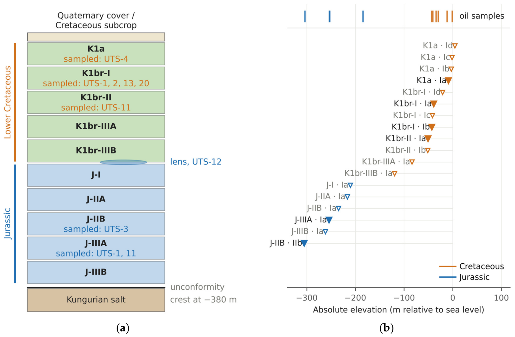
The field contains 18 mapped oil pools in ten named reservoir horizons, with adopted oil–water contacts from +4.5 m to −305.3 m (Figure 5b; Table A1). Six of those mapped pools were sampled for the work reported here. A seventh sampling unit, an isolated upper Jurassic sand lens tested in UTS-12, carries oil but has no mapped contact and is not counted among the 18 mapped pools; in the statistics it is treated as a seventh pool, so the seven sampled units are the clustering units. All mapped pools are structural traps, most of them fault-bounded. The field has never been produced and is currently shut in. All fluids described here were sampled during appraisal tests of cased and cemented wells (Section 3.1).
Figure 3.
Structure of the Uytas salt dome and its supra-salt southern limb. (a) Fault blocks at the Lower Cretaceous marker, closure contoured at −110 m; the outline is drawn to the scale bar, fault positions inside it are schematic, and bold block labels are those sampled. (b) Length × width of the closing contour at the three mapped supra-salt horizons, with dimensions and amplitude, all approximate (Section 3.2). (c) North–south section through the salt body; annotated salt elevations are mapped values, the vertical scale is true and the horizontal distance is schematic. Blue lines are the adopted oil–water contacts.
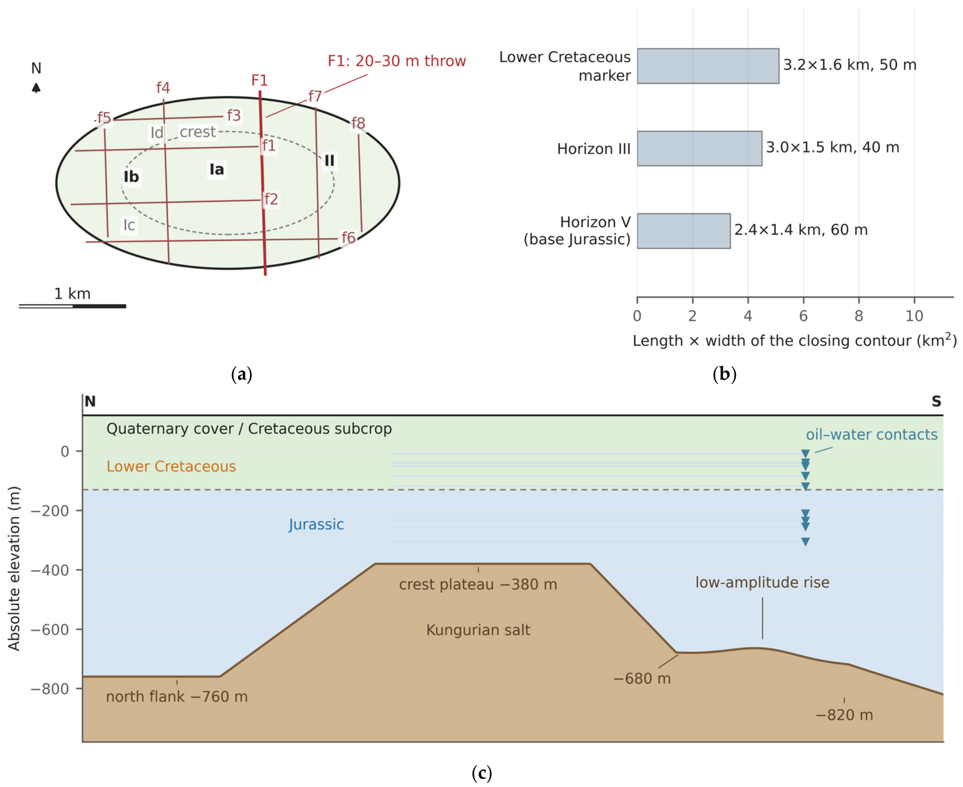
Figure 4.
Seismic sections through well UTS-1 from the field documentation, in two-way travel time (s): (a,b) line 11487, south-west to north-east, uninterpreted and interpreted; (c,d) line 4714, south to north. The red bar marks UTS-1 down to its bottom hole, labelled −828; the horizon and fault interpretation is tied to this well (Section 3.2); line 11487 spans traces 2100–4800 and line 4714 traces 11000–11850.
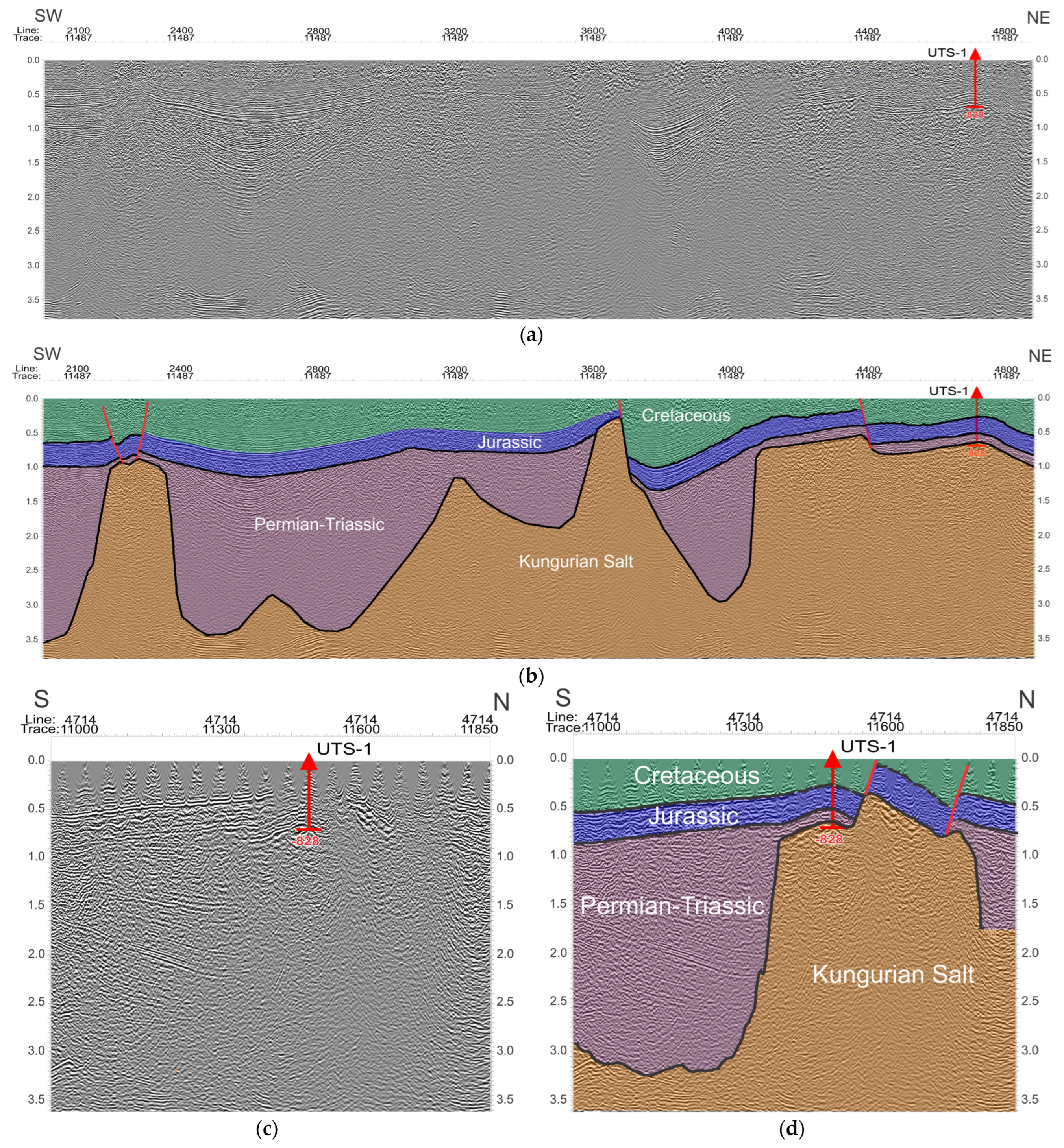
Figure 5.
Stratigraphic framework and pool elevations. (a) The ten named reservoir horizons, not to vertical scale, with the wells sampled from each; the lens marked in the Jurassic is the isolated sand body tested in UTS-12, for which no oil–water contact is defined. (b) Every adopted oil–water contact on a common elevation datum, with the ten oil samples as ticks above; filled symbols are sampled pools, open symbols unsampled, and the horizontal bar is the reported range of an inclined contact.
3. Materials and Methods
3.1. Dataset and Sampling Design
The dataset comprises ten oil samples from eight wells and fifteen formation-water analyses from eight wells; four wells were sampled for both fluids, so twelve wells are represented (Table 1). The oil samples come from six Lower Cretaceous intervals with mid-depths between 110 and 169 m and four Jurassic intervals with mid-depths between 312 and 430 m, referred to below as the two complexes. No oil was sampled between 169 and 312 m, so the two groups are separated by an unsampled interval; whether the change across it is a step or a continuous gradient is examined in Section 5.1. Figure 5a places the sampled horizons in the stratigraphy, Figure 5b places every pool on a common elevation datum, Figure 6a gives the depth of every oil sample and water analysis, and Figure 6b locates the twelve wells. Table 2 is the sample register: for each sample it gives the fault block, the sampled interval, the elevation of its midpoint, the contact adopted for its pool, the height above that contact, the reservoir temperature and the sampling date.
Table 1.
Datasets used in this study. Depths are measured below the rotary table; contacts are elevations relative to sea level.
Table 2.
Oil samples: Location, geometry, reservoir temperature and sampling date. Interval and elevation are in metres, elevation relative to sea level; Δz is the height of the sample mid-depth above the contact adopted for its pool, in metres; T is the reservoir temperature in °C, with the reported range in brackets where one was given. Every depth is a measured depth below the rotary table.
Figure 6.
Sample distribution and well locations. (a) Depth of every oil sample and water analysis in each of the twelve wells: bars span the tested interval and symbols mark its mid-depth, filled for oils and open for waters; the grey band is the interval between the deepest Cretaceous and the shallowest Jurassic oil sample, in which no oil was sampled. (b) Wells of the Uytas field and the 3D seismic survey acquired in 2011 (blue); filled circles are the twelve sampled wells, UTS-1 to UTS-4, UTS-10 to UTS-16 and UTS-20, open circles other wells, and the inset enlarges the framed area.
Of the fifteen water analyses, twelve come from the reservoir intervals compared here, six from each complex; two come from the Albian, a shallow non-productive aquifer, and one from a Triassic interval below the studied section, used as a control. The two complexes are not sampled with the same well coverage. The six Cretaceous reservoir analyses come from six different wells, whereas the six Jurassic analyses come from three wells, three of them from UTS-1 alone. Every water comparison is therefore reported twice, once over the analyses and once over the well means (Section 4.5, Table A7).
Three water analyses come from the same perforated interval as an oil sample: UTS-1 K1br-I, UTS-1 J-IIIA and UTS-3 J-IIB. For UTS-3 J-IIB the oil and the water were sampled on the same day, 15 June 2012, and reported together; for the two UTS-1 intervals the waters were sampled during the testing of the same interval, in December 2010 and January 2011. For the remaining seven oil samples no water from the same interval exists; what the three pairs can and cannot show is examined in Section 5.3.
All oil and water analyses were made between 2010 and 2013 in one accredited laboratory. Sampling dates are given in Table 2 and Table A8: the samples were taken between December 2010 and December 2013. The UTS-3 J-IIB oil and water reached the laboratory five days after sampling; storage conditions between sampling and analysis are not recorded in the laboratory reports. The determinations and the standard method of each are listed in Table 3; kinematic viscosity was measured with calibrated glass capillary viscometers under GOST 33-2000 [40] for four samples and ST RK ASTM D445-2011 [41] for the other six. All determinations are single measurements, so the figures carry no error bars. Where a value is derived rather than measured, that is stated at the point of use and in the table footnotes.
Table 3.
Determinations made on the oil samples and the standard method used for each. All were made in one accredited laboratory (Section 3.1).
Completion and sampling: Intervals were tested in the cased and cemented hole after a cement-bond log. They were perforated at 15–20 shots per metre, depth-tied by gamma ray and casing-collar locator, with guns run on wireline in a completion fluid of 1.04 g cm−3 or on tubing underbalanced. Flow was induced by swabbing or by progressive-cavity pumps at 50–400 rpm and metered on a three-phase separator, from which both fluids were sampled at the wellhead during flow; gas was too scarce to be metered. Three consequences follow. First, each interval was flowed through the separator before it was sampled, so mud filtrate that entered the formation during drilling would have been produced ahead of the sampled fluid, and the intervals were perforated in completion fluid, not in drilling mud. Second, separator sampling removes light ends and so raises density and viscosity, more so in the shallower, lower-pressure intervals, that is, in the direction of the contrast reported in Section 4.2. The oils carried little gas, and the fraction boiling below 300 °C does not differ detectably between the complexes (Section 4.3); both argue against a large differential loss. Because any such loss acts in the direction of the contrast, the reported contrast is an upper bound on the part attributable to the oils themselves. Third, for the waters, degassing of CO2 and H2S at the separator can lower hydrogen carbonate, calcium and dissolved sulfide and raise pH, but leaves sodium, chloride and bromide unchanged and cannot produce the sodium excess over chloride of the shallow waters (Section 4.5); a completion fluid of 1.04 g cm−3 corresponds to about 50–60 g L−1 of dissolved salt, more than any Lower Cretaceous reservoir water (7.4–31.4 g L−1), so a residue of it would raise rather than lower the salinity of the shallow waters.
3.2. Seismic Data and Structural Framework
The structural framework rests on a 3D survey over the northern part of the licence area and a later, higher-fold 3D survey of 26.83 km2 over the southern limb, processed through pre-stack time migration. Interpretation was tied to well UTS-1, which penetrates the full supra-salt section. Four horizons were mapped: the top of the salt, the base of the Jurassic, an intermediate Jurassic reflector and a Lower Cretaceous marker. The displays in Figure 4 are in two-way travel time; depth conversion used the well-tie velocities and is the basis for the structural elevations quoted in Section 2.
The depth conversion affects only the structural numbers of Section 2. A 2% velocity error at 600 m is 12 m, which is 20–30% of the closure amplitudes of 40–60 m. For an elliptical closure with a uniform flank dip, the dimensions and amplitudes in Section 2 imply flank gradients of 38–65 m km−1, so a 12 m depth error moves the closing contour by 0.18–0.32 km and changes the closed area by roughly 35–70%. The closure dimensions, areas and amplitudes are therefore approximate values. No result in Section 4 and Section 5 depends on them: the contacts, sampled intervals and heights above contact are picked on well logs (Section 3.4, Table A1).
Two further points follow from the survey geometry. First, the 3D coverage stops at the edge of the oil fields, so the periphery of the salt body and its junction with the neighbouring salt structures are unresolved and the eastern flank of the diapir is not imaged; the salt saddles shown in Figure 2 lie in that unresolved zone, and that sketch is schematic and carries no horizontal scale. Second, the individual reservoir units, at 100–450 m, are close to or below the vertical resolution of the data, so they are not separable seismically and the correlation between wells rests on logs rather than on seismic character. The assignment of wells to fault blocks likewise rests on log correlation and on the pressure and contact data, not on seismic fault picks.
3.3. Viscosity: Measurement, Fitting and the Quantities Derived from It
Kinematic viscosity was determined at 20, 30, 40, 50 and 100 °C, giving five determinations for each of the ten samples. Each series was described by the viscosity–temperature relation of ASTM D341 [52], Equation (1):
Here ν is the kinematic viscosity in mm2 s−1, T the absolute temperature in kelvin, and A and B the two constants fitted to each sample; both logarithms are decimal. The exponential correction terms of the standard’s Z are below 1 × 10⁻⁷ mm2 s−1 for the smallest determination in this dataset, 6.18 mm2 s−1 (Table A2), and are omitted. A and B were obtained by ordinary least squares of log10 log10 Z on log10 T; the fitted constants and the fifty determinations behind them are given in Table A2 and Table A3. Inverting Equation (1) gives the viscosity at any temperature within the fitted range, Equation (2):
The ten fitted relations and the determinations that constrain them are shown in Figure 7a. Per-point residuals rather than the coefficient of determination alone are reported, because a single inconsistent determination is invisible in R2 (Figure 7b). The median absolute residual over the fifty determinations is 1.15%.
Figure 7.
ASTM D341 fits and the cost of extrapolating them. (a) The ten fitted viscosity–temperature relations with the laboratory determinations that constrain them, crosses; circles are the value at reservoir temperature and the shaded band the range of reservoir temperatures. (b) Per-point fit residuals, % of the measured value. (c) Reservoir temperature of each sample against the lowest measured temperature, dashed line at 20 °C; red segments mark fits extrapolated below the measured range, and the labels give the change in estimated viscosity for a 1 °C error in reservoir temperature.
Dynamic viscosity follows from the kinematic value and the density by the defining relation, Equation (3):
with ρ in g cm−3 and ν in mm2 s−1, giving μ in mPa·s. The dynamic viscosity at 20 °C, printed in Table 4, is the product of two measurements, the density and the kinematic viscosity at 20 °C, and involves no model. The dynamic viscosity at reservoir temperature is read from the fitted curve through Equation (2), with the density at 20 °C, and is a model value; a density reduced to reservoir temperature would change it by less than 0.5%. Ratios are formed only between quantities on the same basis, and the measured and fitted bases are carried side by side in Table A3.
Table 4.
Oil samples: Bulk physical properties. The first four columns are measurements and quantities computed directly from them; the last column is modelled. Units: ρ20, density at 20 °C, g cm−3; ν20, kinematic viscosity at 20 °C, mm2 s−1; μ20, dynamic viscosity at 20 °C, mPa·s; T, reservoir temperature, °C; μ at T, dead-oil dynamic viscosity at T, mPa·s.
Comparisons at a common temperature use the fitted curves for both groups, because the in-situ values exist only on those curves; Table A3 gives the measured value, the fitted value and the residual of each sample.
One sample, UTS-1 J-IIIA, departs from the D341 form: its determinations at 30 and 20 °C have residuals of +19.3% and −12.2%, and the ratio of its determinations at 40 and 30 °C, 0.785 against a median of 0.563 for the other nine, has a robust z score of 8.1. It is retained; refitting it without the 30 °C determination, or removing it, are among the alternatives of Section 4.2.
Every reservoir-temperature viscosity in this paper is an estimated dead-oil value read from the fitted curve at the temperature reported for the pool. A live-oil viscosity, which would be lower, is not estimated, because the correlation that gives it [53] requires a solution gas–oil ratio; all comparisons are between dead-oil values obtained the same way.
For the six Cretaceous samples the fit is extrapolated below the lowest measured temperature, by up to 6.3 °C; the four Jurassic reservoir temperatures lie inside the measured range (Figure 7c). Sensitivity to reservoir temperature is 5.1–8.8% per °C, and temperature-error scenarios are carried through Section 4.2. All ten pour points are reported as −20 °C, below every reservoir temperature.
3.4. Density, API Gravity and Sample Geometry
API gravity is defined at 60/60 °F, so the measured density at 20 °C must first be reduced to the 60 °F base. The reduction follows the crude-oil procedure of API MPMS Chapter 11.1, published jointly as ASTM D1250 [54], Equation (4):
where ρ(T) is the density at the temperature of measurement, ρ60 the density at the 60 °F base, ΔT the difference T − 60 in degrees Fahrenheit and α60 the thermal-expansion coefficient at the base temperature, in reciprocal degrees Fahrenheit. For crude oil the standard sets K0 = 341.0957 with the two higher coefficients zero, and ρ60 is expressed in kg m−3. Because α60 itself depends on ρ60, Equation (4) is inverted numerically for each sample. API gravity then follows from its definition, Equation (5):
with ρw = 0.999016 g cm−3, the density of water at 15.56 °C. Over the density range of these samples, 0.883 to 0.906 g cm−3, the procedure corresponds to an effective relative expansion coefficient of 7.47 to 7.86 × 10⁻⁴ K−1 and gives 24.01 to 28.03 °API; the reduction from 20 to 15.56 °C changes API gravity by about 0.5 °API and is applied because the classification thresholds are defined at 60 °F [55,56]. API gravity is therefore a deterministic function of density, not an independent property (Section 3.7).
The height of each oil sample above its own oil–water contact is a geometric quantity defined for this study rather than a published index, and it is stated here as a definition, Equation (6):
where Ei is the rotary-table elevation of the well that produced sample i, the mid-depth i the mid-depth of the sampled interval measured from the rotary table, and EOWC(i) the contact elevation adopted for the pool and fault block from which that sample came (Table A1). All three terms are in metres relative to sea level, and a positive height places the sample above its contact. Measured depth is taken as true vertical depth in these shallow vertical wells. Heights are quoted to 0.1 m, as their inputs are, and their meaning depends on how the contact was picked: a direct oil–water contact on logs gives a measured height, the base of an oil-saturated bed a lower bound, the top of a water-saturated bed an upper bound, and a midpoint between picks in two wells a height read as at the contact (Section 4.7, Table A1).
3.5. Formation-Water Analyses and Hydrochemical Indices
Waters were analysed for chloride, sulfate, hydrogen carbonate, carbonate, calcium and magnesium, together with total dissolved solids (TDS), residue on evaporation, pH and specific gravity; bromide, iodide and hydrogen sulfide were determined on part of the set (Table A8). Carbonate is below the reporting limit in fourteen of the fifteen analyses and is 0.4 mg L−1 in the fifteenth. Sodium plus potassium was obtained by the laboratory as the difference between total anions and calcium plus magnesium, the convention of the standard method used, and is reported as a sodium equivalent.
Two consequences follow. First, the charge balance of every analysis is closed by construction: recomputing the difference reproduces the reported sodium within 0.19 meq L−1, the rounding of the reported value, so the charge balance is not used as a check on analytical quality (Figure A1a; Figure A1b,c check the viscosity data). The water analyses are checked instead against the residue on evaporation (below and Table A8). Second, any index containing sodium inherits the uncertainty of the five measured ions.
The genetic classification and the ionic ratios are computed on equivalent concentrations. For an ion X of molar mass M and charge number z, the equivalent concentration used throughout is given by Equation (7):
where c is the mass concentration in mg L−1 and E is the equivalent mass, the molar mass divided by the absolute value of the charge number, so that r X is in meq L−1. The three indices reported in Section 4.5 are then the dimensionless ratios of Equation (8); the first two, with (rNa − rCl)/rSO4 below, are the criteria of the Sulin genetic classification [57]:
The first ratio divides sodium-type from chloride-type waters at unity; among the sodium-type waters, the sulfate–sodium (Na2SO4) type has (rNa − rCl)/rSO4 below one and the hydrogen-carbonate–sodium (NaHCO3) type above one [57]; here the values are 0.07–0.83 and 1.9–19.8. The second separates the two chloride types, also at unity: a value below one is the chloride–magnesium (MgCl2) type and a value above one the chloride–calcium (CaCl2) type, which is the boundary applied in Section 4.5. The third is the sulfate index, scaled by 100. The consequence of obtaining sodium by difference is sharpest in the Jurassic. All six Jurassic reservoir waters lie close enough to the chloride–calcium against chloride–magnesium boundary that a shift in sodium of less than 2% of chloride would move it across, the smallest such shift being 0.2%. The first-order division, sodium-type against chloride-type, is robust; the assignment between the two chloride types is not resolved by these data.
Total dissolved solids were recomputed as the sum of the reported ion masses, including the sodium obtained by difference, and reproduce the TDS reported by the laboratory. The residue on evaporation determined by the laboratory is an independent check: with hydrogen carbonate converted to carbonate [58], it exceeds the sum of ions in fourteen of the fifteen analyses, with a median departure of +4.6%, and agrees with it within 10% in eleven; the largest departures, +21 and +31%, are in two UTS-1 analyses (Table A8).
pH was determined on all fifteen waters, at 7.4–7.8 in ten and above 8 in five; bromide and iodide were determined on four and dissolved hydrogen sulfide on nine, in which it was detected twice, at 85 and 106 mg L−1 (Table A8). Sampling effects on the waters are set out in Section 3.1.
3.6. Group Contrasts and Their Decomposition
The quantity to be estimated is the ratio of the group mean dead-oil dynamic viscosity at reservoir temperature between the Lower Cretaceous and the Jurassic complexes. Two ratios are reported and are not interchangeable. The ratio of arithmetic means, Equation (9), is the quantity a volumetric average would use:
and the ratio of geometric means, Equation (10), is the quantity the log-transformed test statistic estimates, because the mean of the logarithm is the logarithm of the geometric mean:
In both, g indexes the two complexes, n is the number of samples in complex g, and the sums run over the samples of that complex. The two ratios answer different questions and differ numerically whenever the within-group spread differs between the groups; both are reported (Table A5), and pairwise ratios within the two wells that sampled both complexes are reported separately again, because a pairwise ratio is not an estimate of either group ratio.
Because the two complexes sit at different reservoir temperatures, part of the observed contrast is a temperature effect and part is not. The two contributions are separated by an algebraic identity, obtained by adding and subtracting the logarithm of each group mean evaluated at a common reference temperature T0, Equation (11):
The first term on the right is the contrast the two groups would show if both were at T0; the second and third together are the contribution of the difference in reservoir temperature. The identity is exact on the fitted curves, but it partitions an observed number and does not show that temperature causes the part attributed to it.
3.7. Statistical Treatment
The null hypothesis is that the label Cretaceous or Jurassic is exchangeable with respect to the measured property. The samples were taken where wells penetrated oil, not assigned at random, so the test asks whether the observed separation exceeds those obtainable by relabelling, not whether the grouping caused it.
One test family is primary throughout. For every property the two complexes are compared by an exact permutation test on the difference in group means, on log10 values for the two viscosities and on the measured values for the other properties, enumerating all C(10,4) = 210 label assignments [59]. The two-sided probability is defined by Equation (12):
where Π is the set of all M = 210 label assignments, S(π) the absolute difference in group means under assignment π, Sobs its observed value, and I the indicator that is one when the inequality holds and zero otherwise. The observed assignment belongs to Π, so the probability is never zero; its smallest attainable value is 1/210 = 0.0048 when one assignment separates the labels more sharply than every other, and every smallest attainable value quoted in this paper was obtained by enumeration. The twelve reservoir waters are compared by the same test on log10 values of every variable, over all C(12,6) = 924 assignments (Section 4.5).
Eleven properties were tested, so the primary probabilities are corrected across the whole family by the Benjamini–Hochberg procedure [60], Equation (13):
where p(1) ≤ … ≤ p(m) are the ordered probabilities of the family of size m and q* is the false-discovery rate controlled. The family of eleven contains at most eight independent quantities, because API gravity is a function of density, the two viscosities share a fit, and saturates, aromatics and resins form a closed composition; the correction is therefore conservative.
Two sensitivity analyses, reported in Table A4, accompany the primary test and are corrected within their own families. Welch’s test for two means with unequal variances [61] is applied to the same transform, Equation (14):
and the Mann–Whitney rank test [62] is applied to the untransformed values, Equation (15), with RC the sum of the ranks of the Cretaceous samples in the pooled ranking:
Effect sizes are Hedges’ g with its small-sample correction [63], Equation (16), where df = nC + nJ − 2:
and Cliff’s delta [64], Equation (17), the difference between the proportion of cross-group pairs in which the Cretaceous value exceeds the Jurassic one and the proportion in which it is smaller:
Both are read as direction rather than magnitude at this sample size: a Cliff’s delta of ±1 means only that the groups do not overlap. The denominator of Hedges’ g for density is of the order of the step at which density is reported, so that value is quoted to one significant figure.
Sample, well and pool are different units of analysis. Within each complex every sample comes from a different well; two wells, UTS-1 and UTS-11, sample both complexes and give the within-well ratios reported in Section 4.2. The repeated unit is the pool: three of the six Cretaceous samples come from K1br-I block Ia and two of the four Jurassic samples from J-IIIA block Ia, so at the pool level the design is four units against three, and the smallest attainable permutation value is 1/C(7,3) = 0.029.
Every correlation is computed on the pooled data and within each complex, and each family of ten is corrected within itself. A coefficient computed across the two complexes measures the separation between them; the term Simpson’s paradox [36] is used only where the within-group coefficient reverses in sign. The p value of a correlation is the exact permutation probability over all n! orderings of the response, and within-group coefficients are also recomputed with each sample removed in turn (Section 4.4).
Regressions are reported with a leave-one-out cross-validated Q2 alongside R2 [65], Equation (18):
where (−i) is the prediction for observation i from the model refitted without it and the denominator is the total sum of squares about the mean of the whole sample, so Q2 < 0 marks a model that predicts worse than that mean. At these sample sizes a negative Q2 is common even for a model that fits: over 40,000 simulated bivariate-normal replicates it occurs in 42% at n = 6 with a population R2 of 0.6 and in 35% at n = 4 with a population R2 of 0.85, so a negative Q2 is read as weak evidence.
Saturates, aromatics and resins sum to 99.83 to 100.00% in the ten samples, and to exactly 100.00% in six of them. Asphaltenes were detected in three samples, at 0.04–0.18 wt %, and reported as absent in the other seven; the four fractions sum to 99.97–100.03% in every sample. The SARA (saturates, aromatics, resins and asphaltenes) composition is therefore closed, and the three fractions are treated as compositional data with two free dimensions, whose mutual correlations are partly forced. Where a compositional comparison matters it is repeated on additive log ratios [66], Equation (19), with resins as the common denominator and no zero values present:
where wk is the mass fraction of component k. The untransformed coefficient between saturates and aromatics is −0.952 and that between their log ratios to resins +0.781, so the untransformed value reflects the closure and is not read as a relation between the two fractions.
4. Results
4.1. Gravity, Viscosity and What the Oils Are
Densities at 20 °C are 0.883–0.906 g cm−3, corresponding to 24.0–28.0 °API (Table 4). The Cretaceous samples span 24.0–25.4 °API and the Jurassic 27.3–28.0 °API. The gravity-based heavy-oil boundary is placed at 22.3 °API by the two classifications used here [55,56], so on that criterion none of these samples is a heavy oil and all ten fall in the medium band (Figure 8a).
Figure 8.
The Uytas oils in gravity–viscosity classification space. (a) API gravity against modelled dead-oil viscosity at reservoir temperature, with the gravity-based classification fields and the 100 mPa·s line that bounds the viscosity-based heavy-oil field. (b) Fitted viscosity–temperature relations for all ten samples; the shaded band is the reservoir-temperature range, 13.7 to 25.2 °C. Orange circles are Lower Cretaceous and blue squares Jurassic throughout this paper.
By the viscosity-based criterion the answer differs. Estimated dead-oil viscosity at reservoir temperature exceeds 100 mPa·s in seven of the ten samples and falls below it in three. The distinction is thermal: warmed to between 20 and 43 °C, every sample in the set falls below 100 mPa·s (Figure 8b). These are therefore medium-gravity crudes that are viscous in place because the reservoirs are cold, and they are described that way here rather than as heavy oils.
In absolute terms, saturate content is 70.4–79.2 wt % in the Cretaceous and 82.3–82.8 in the Jurassic; total sulfur is 0.100–0.174 and 0.070–0.100 wt %. Asphaltenes are below 0.2 wt % in the three samples in which they were detected and were reported as absent in the other seven. On absolute composition both groups are saturate-rich and low in sulfur, and neither group has the bulk composition of a strongly altered oil.
4.2. The Vertical Contrast and Its Decomposition
Estimated dead-oil viscosity at reservoir temperature is 234–764 mPa·s in the Lower Cretaceous and 83–112 mPa·s in the Jurassic, with group means of 429 and 94.9 mPa·s. Density falls from a Cretaceous median of 0.901 to a Jurassic median of 0.885 g cm−3 and API gravity rises correspondingly. Saturate content rises from 70.4–79.2 to 82.3–82.8 wt %, aromatics fall from 15.2–21.0 to 11.3–14.8, resins from 5.2–8.5 to 2.9–6.0, and total sulfur from 0.100–0.174 to 0.070–0.100 wt % (Table 5, Figure 9 and Figure 10). All these changes are in the direction that separates a more-altered from a less-altered oil, and Section 5.2 asks whether their magnitude is consistent with that reading.
Figure 9.
Depth profiles of six measured oil properties: (a) Kinematic viscosity at 20 °C, (b) API gravity, (c) total sulfur, (d) saturates, (e) aromatics, and (f) resins. Symbols are single determinations, so no error bars can be drawn. The shaded band marks the interval between the deepest Cretaceous and the shallowest Jurassic oil sample, 169–312 m, in which no oil was sampled.
Figure 10.
SARA composition of the ten oils. (a) Magnified projection of the saturate–aromatic–polar ternary; on the full diagram all ten samples fall in one corner. Sample identities are in panel (b). (b) The same compositions as stacked bars, ordered by modelled viscosity at reservoir temperature with the most viscous at the top. Saturates, aromatics and resins are closed to 100%, so their mutual correlations are partly forced.
The ratio of group mean dynamic viscosities at reservoir temperature is 4.52, with exact permutation p = 0.0048, the smallest value the design can return (Figure 11b). Across the sample-level alternatives of Table A5, namely the median or the geometric mean instead of the arithmetic mean, a 1 °C error in reservoir temperature applied to both complexes or in opposite directions, removal of each of the four most influential samples, refitting UTS-1 J-IIIA without its 30 °C determination, and one sample per well, the ratio stays between 3.81 and 5.30 (Figure 11c).
Figure 11.
How large the in-situ viscosity contrast is and how well it is resolved. (a) The contrast at three levels of the design: Sample means, pool means, and the two wells that sample both complexes. (b) The exact permutation null for the group difference in mean log10 viscosity over all 210 label assignments; the solid line is the observed difference and the dashed line its mirror. (c) Every alternative estimate of the same quantity, ordered by value, with the baseline as a vertical line.
At the pool level, the clustering unit of the design, the ratio is 4.74 on four pools against three, with p = 0.029, the floor of that design (Section 3.7). The two wells that penetrate both complexes, UTS-1 and UTS-11, give within-well ratios of 3.78 and 2.37 (geometric mean 3.00; Figure 11a), and within one pool, K1br-I block Ia, three samples span a factor of 1.35.
How much of the contrast is the oil rather than the temperature is a separate question, and the answer depends on the reference temperature chosen. Compared at a common 20 °C, in dynamic viscosity read from the fitted curves of both groups, the two groups differ by a factor of 2.40; at 25 °C the factor is 2.25 and at 30 °C it is 2.13. On the measured values at 20 °C, the basis of the dynamic viscosity printed in Table 4, the same comparison gives 2.34. The decomposition below uses the fitted basis (Section 3.3).
The decomposition is multiplicative rather than additive: at a 20 °C reference, 4.52 is approximately 1.89 times 2.40, the first factor arising from the reservoirs being at different temperatures, 13.7–19.8 °C in the Cretaceous against 22.8–25.2 °C in the Jurassic, and the second from the difference between the oils. On a logarithmic scale the thermal factor accounts for about 42% of the in-situ contrast at that reference. Because the compositional factor falls as the reference temperature rises, neither that percentage nor the factor 2.40 is a property of the field alone: both are defined relative to a chosen reference and must be quoted with it.
4.3. Which Properties Separate the Complexes
Of the eleven properties tested, eight differ between the complexes at a false-discovery rate below 5% under the primary test (Table 6). Six do so clearly (q = 0.013–0.017): density and API gravity, which are one measurement; the two viscosities, which share a fit; and saturates and aromatics. Total sulfur and resins are marginal (q = 0.045 and 0.046), each separating under only one of the two sensitivity tests (Table A4). Cliff’s delta is ±1.00 for the six, so the groups do not overlap on these properties.
Table 5.
Oil samples: SARA composition and related determinations. Saturates (Sat.), aromatics (Arom.), resins (Res.), asphaltenes (Asph.), total sulfur (S) and paraffin (Wax) in wt %; molecular mass (M) in g mol−1; the fraction boiling below 300 °C in vol %.
Paraffin content, molecular mass and the fraction boiling below 300 °C do not separate the complexes (q = 0.230, 0.230 and 0.390; Table 6, footnote 5). Paraffin is among the first components biodegradation removes, so its failure to separate the groups limits how far any alteration can have gone.
4.4. Correlations Within and Across the Complexes
Computed on all ten samples, total sulfur and saturate content correlate with log10 viscosity at 20 °C at r = 0.864 and −0.836 (exact permutation p = 5.0 × 10⁻⁵ and 0.0041), and the saturate regression has R2 = 0.70 and Q2 = +0.54. Within each complex the saturate relation disappears (R2 = 0.13 and Q2 = −0.50 in the Cretaceous, R2 = 0.01 and Q2 = −2.60 in the Jurassic), and the sulfur coefficients, although high (r = 0.857 and 0.922), are not resolved: after correction no within-group coefficient survives (smallest q = 0.25 in the Cretaceous and 0.42 in the Jurassic; Table A6, Figure 12a,b), and the Cretaceous sulfur coefficient falls to +0.57 when one sample is removed (Figure 12d). The pooled coefficients therefore describe the separation between the complexes; regression diagnostics and the full coefficient matrices are in Figure A2 and Figure A3.
One within-group coefficient reverses in sign. Within the Jurassic, sampling depth correlates with log10 viscosity at r = 0.967 (parametric p = 0.033, n = 4), whereas the pooled coefficient for the same pair is −0.830 (Figure 12c), which is Simpson’s paradox in the strict sense [36]. The exact permutation p over all 24 orderings is 0.083, against a smallest attainable value of 0.042, so four points do not resolve the relation; the coefficient stays between +0.94 and +0.99 when any one sample is removed. With four points from three pools it shows that viscosity varies within the Jurassic as well as between the groups, and Section 5.1 uses it only to test a single monotonic depth trend.
4.5. Formation Waters
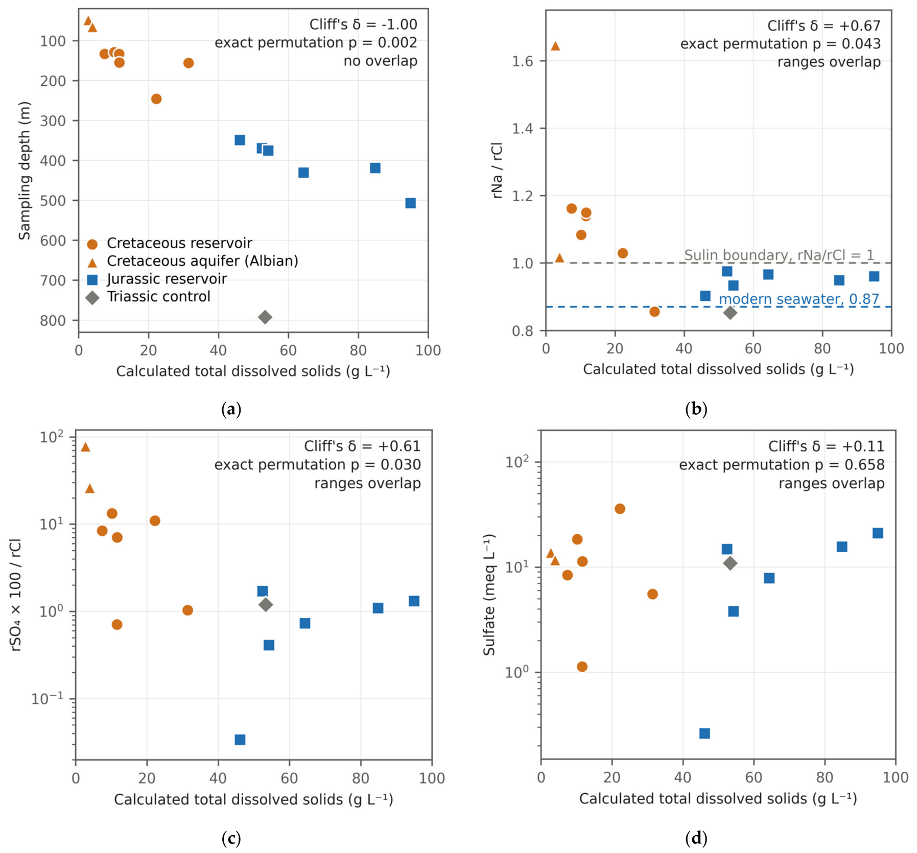
Cretaceous reservoir waters have 7.4–31.4 g L−1 total dissolved solids; the two Albian aquifer samples above them have 2.7–3.9 g L−1; Jurassic reservoir waters have 46.1–94.9 g L−1, and the Triassic control sample at 792.5 m has 53.3 g L−1 (Table 7 and Table 8, Figure 13a). Salinity, measured here by TDS, rises strongly with depth through the studied section and falls again below it, but not monotonically, with three inversions within the section: between 133.3 and 133.5 m (11.6 to 7.4 g L−1), between 156.0 and 245.9 m (31.4 to 22.2 g L−1) and between 419.0 and 430.5 m (84.8 to 64.3 g L−1).
Under the exact permutation test on log10 values (Section 3.7), total dissolved solids and absolute chloride separate the complexes completely (Table A7, Figure A4a; Cliff’s delta −1.00, p = 0.0022, q = 0.006); chloride is the dominant anion in every analysis, so the two are one salinity signal. The separation survives at the well level (q = 0.036). Nothing else separates the complexes after correction. The sulfate-to-chloride ratio, the index on which a flushing interpretation would rest, gives p = 0.030 under the primary test and 0.093 under a rank test, with overlapping ranges and Cliff’s delta +0.61, and q = 0.061, or 0.238 at the well level. Absolute sulfate does not separate the complexes (medians 9.85 and 11.4 meq L−1, Cliff’s delta +0.11, p = 0.66; Figure 13c,d and Figure A4b, Table A7), and the sodium-to-chloride ratio crosses unity between the complexes without separating them (Figure 13b).
Not everything in these waters is dilution, however. Dilution preserves ion ratios exactly. Taking geometric means of the ion-to-chloride ratios in the two sets of reservoir waters, sulfate departs by a factor of 7.9 and hydrogen carbonate by 4.2, while sodium departs by 1.12 and magnesium by 0.81. Sodium relative to chloride crosses unity between the groups, from 0.86–1.16 in the Cretaceous to 0.90–0.98 in the Jurassic, and no amount of dilution can move a ratio across that line. At least three ions are therefore non-conservative. Five of the six shallow reservoir waters carry sodium in excess of chloride, and the three hydrogen-carbonate–sodium waters also carry less calcium relative to chloride (rCa/rCl 0.009–0.012) than any Jurassic (0.016–0.025) or Albian (0.22–0.23) water; that is the pattern base exchange in a freshening aquifer would produce.
By the Sulin classification the shallow waters are sulfate–sodium and hydrogen-carbonate–sodium types with one exception, and the Jurassic waters are chloride-type (Table 8; the full ion patterns are in Figure A5). The exception matters: the water from UTS-1 K1br-I at 156.0 m is a chloride–calcium type, the most saline water in the Cretaceous set at 31.4 g L−1, with a sulfate-to-chloride ratio of 1.03 that lies inside the Jurassic range.
The three perforated intervals that yielded both an oil and a water sample are the only sample-level indication available. The two Jurassic pairs combine less-altered oils with saline, sulfate-poor waters. In the Cretaceous pair the UTS-1 K1br-I oil is a fully Cretaceous-type oil at 327 mPa·s with 72.5 wt % saturates, and the water from the same tested interval is the most saline and least flushed water in the Cretaceous set, although fresher than every Jurassic water. Their association is tested in Section 5.3.
Table 6.
Comparison of the two complexes under the primary test, six Cretaceous samples against four Jurassic ones throughout. Each group column gives the median with the range in brackets. p is the exact two-sided permutation probability on the difference in group means, on log10 values for the two viscosities and measured values otherwise, enumerated over all 210 label assignments; q is p corrected across the family of eleven properties by the Benjamini–Hochberg procedure; g is Hedges’ g, Equation (16), on the same values; δ is Cliff’s delta.
4.6. Present-Day Temperature and Pressure
Eight bottom-hole temperatures are available, between 138.4 and 393.4 m. A least-squares fit gives 3.41 ± 1.49 °C per 100 m (95% confidence interval) with R2 = 0.84 and p = 0.001. Seven of the eight measurements lie between 130 and 200 m; the eighth, at 393.4 m, has leverage 0.95 and a Cook’s distance of 3.72 against a conventional threshold of 0.5 [67], and removing it changes the slope to 1.87 ± 7.15 °C per 100 m with p = 0.53 (Figure A9a,b). The gradient therefore enters Section 5.5 as a range of assumed values.
Twenty-four formation pressures between 121.5 and 485 m give a gradient of 0.9867 ± 0.0140 MPa per 100 m (R2 = 0.9990), close to hydrostatic for the densities of the formation waters (Figure A9c).
4.7. Sample Geometry Relative to the Oil–Water Contacts
Because biodegradation is concentrated at the oil–water contact and its effects diminish upward [17], a sampling artefact is a possibility: if the Cretaceous samples happened to come from close to their contacts and the Jurassic samples from high in their columns, the contrast could be a geometry effect. The geometry is the opposite of that. Cretaceous samples sit 1.8–27.2 m above their own contacts; the three Jurassic samples with a defined contact sit 0.5 to 1.6 m above theirs, within the uncertainty of the contact elevations, and they are the less-altered oils in the field (Figure A6). Within the Cretaceous there is no relation between height above the contact and log10 viscosity at reservoir temperature (r = −0.066, exact permutation p = 0.849 on six samples), and none over the nine samples that have a mapped contact (r = +0.443, p = 0.247).
Figure 12.
Correlations computed on the pooled data measure the separation between the complexes. (a,b) Two of the strongest pooled relations, pooled fit dashed and the two within-complex fits solid; printed values are Pearson r with the exact permutation p in brackets on 10, six and four samples. (c) Sampling depth against viscosity, the pair with the largest within-group coefficient that reverses in sign against the pooled fit. (d) Leave-one-out test on the within-complex coefficients of five properties: symbol, the coefficient on all samples; bar, the range over all leave-one-out fits; red tick, the value closest to zero.
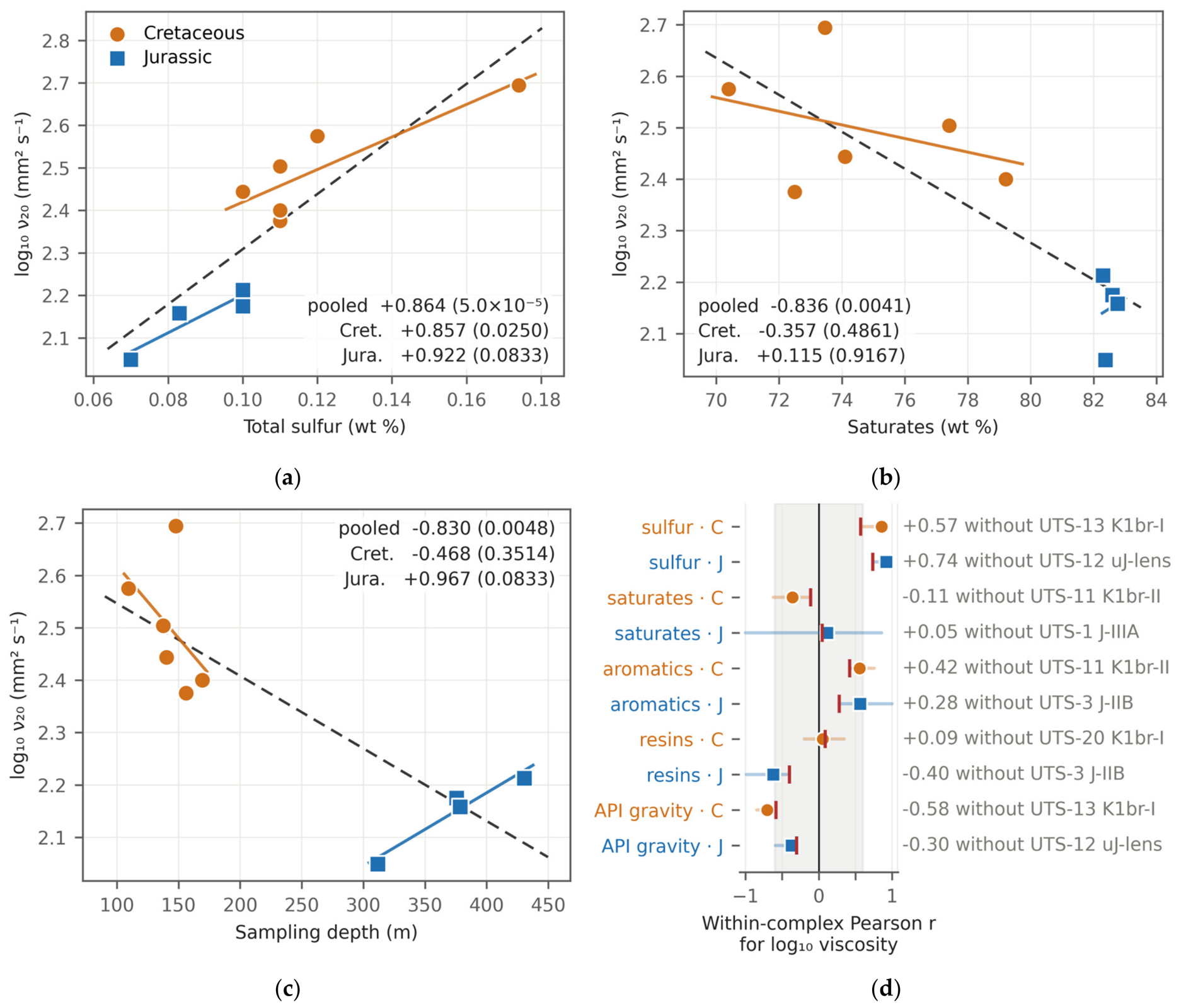
Figure 13.
Formation waters. (a) Salinity against depth; salinity rises through the studied section but not monotonically. (b) rNa/rCl, (c) rSO4 × 100/rCl and (d) absolute sulfate, each against salinity. Every panel carries Cliff’s delta and the exact permutation p over the twelve reservoir analyses, six per complex; the Albian aquifer and Triassic control samples are plotted but excluded from the tests. Only salinity separates the complexes.
The geometry therefore excludes the simplest sampling artefact, in which the more-altered samples are those taken nearest their contacts. The heights differ in kind between pools, because only one of the six sampled contacts is a direct oil–water contact on logs (Section 3.4); UTS-1 J-IIIA, 0.5 m above a contact defined as the midpoint between picks in two wells across a 3.1 m oil column, is read as at the contact.
Table 7.
Formation waters: Measured ion masses. Depth in metres; ion masses in mg L−1; TDS in g L−1. Setting: LC, Lower Cretaceous; J, Jurassic; Tr, Triassic. Twelve analyses come from the reservoir intervals compared here, six from each complex; two are from the Albian, a shallow non-productive aquifer, and one is a Triassic sample from below the studied section.
Table 8.
Formation waters: Genetic indices and classification. TDS in g L−1; the indices are dimensionless ratios of milliequivalent concentrations. Setting as in Table 7. Equivalent weights: Cl 35.453, SO4 48.030, HCO3 61.017, CO3 30.005, Ca 20.039, Mg 12.153, and Na 22.990.
5. Discussion
5.1. What the Data Establish
Section 4 establishes three results: the two groups of oils do not overlap in density, API gravity, viscosity, saturates or aromatics; the in-situ viscosity contrast holds at the sample, pool and well levels; and at a 20 °C reference about 42% of it, on a logarithmic scale, is thermal (Section 4.2 and Section 4.3). The decomposition does not identify which property of the oils produces the remainder (Section 5.2).
The unsampled interval between 169 and 312 m bears on how the contrast is described. Fitted to all ten samples, a linear trend of log10 viscosity at reservoir temperature against depth and a model with one mean per complex, both with two parameters, fit almost equally well (R2 = 0.80 and 0.86; leave-one-out Q2 = +0.68 and +0.79), so the aggregate fit alone does not exclude a continuous gradient. Two observations favour a stratigraphic step. The oil from the upper Jurassic lens in UTS-12, at 311.8 m and 22.8 °C, intermediate in depth and temperature, has Jurassic-type properties (saturates 82.4 wt %, density 0.884 g cm−3, total sulfur 0.07 wt %) and the lowest in-situ viscosity in the field, 83.0 mPa·s, against 158 mPa·s predicted by a depth trend through the other nine samples, a residual of −1.9 residual standard deviations of that fit. Within the Jurassic, viscosity rises with depth on four samples (Section 4.4), which a single monotonic trend would not produce. In UTS-12 the water at 245.9 m still has a Cretaceous salinity (22.2 g L−1; Table 7) and the oil at 311.8 m has Jurassic-type properties, so in that well a change common to both fluids would lie between about 247 and 311 m. Across the field the depth at which the change occurs is not resolved by these data.
5.2. In-Reservoir Alteration, and What Competes with It
The direction of every compositional difference is the direction in-reservoir biodegradation produces: saturates down, aromatics and polars up, density up, and viscosity up [14,15,16]. The shallow reservoirs also satisfy some of the conditions degradation requires: they are cold but not too cold, and they subcrop beneath Quaternary cover so a recharge path exists.
Biodegradation is diagnosed molecularly [23,24], and the process inferred here from bulk data is therefore referred to as in-reservoir alteration. The bulk compositions of both groups (Section 4.1) are in the range reported for crudes that have undergone little alteration, consistent with slight alteration of the Cretaceous oils. Absolute sulfate does not differ between the groups (Section 4.5), and single concentrations do not measure sulfate flux; methanogenic degradation, regarded as dominant in many reservoirs [68], requires no sulfate.
Three further processes reproduce part of the same bulk pattern. Charges of one source arriving at different times and maturities would also differ in saturate content, sulfur and density, and would produce a depth-ordered pattern if the shallower reservoir received the earlier or less mature charge [25]. Water washing acts first on the fraction lighter than about C15 and on aromatic and sulfur compounds [22]; the Cretaceous oils are not detectably depleted in the light fraction and are richer, not poorer, in aromatics and sulfur, so washing is subordinate. The third, a differential loss of light ends during separator sampling, is bounded in Section 3.1; molecular mass, which such a loss would raise, does not differ detectably either (Table 6). Of the three processes, a multi-stage charge of the same oil remains substantive; it can be separated from alteration in place only with molecular and isotopic data [23,24,26].
Two observations bound the alteration from inside the dataset. Paraffin content and the fraction boiling below 300 °C respond early to biodegradation, through the loss of n-alkanes and light compounds [23,24], and molecular mass responds with them; none of the three separates the complexes, although their medians differ in the same sense as the separating properties (Table 6). The Cretaceous oils are therefore either slightly altered or partly degraded oils replenished by a later charge of the same oil [16,17,25].
The second is quantitative. The compositional difference between the groups amounts to about nine points of saturates, five of aromatics and three of resins, with a density difference of 0.016 g cm−3 between the group medians, and it accompanies a factor of about 2.40 in dynamic viscosity at a 20 °C reference (Section 4.2). For the group mean gravities, the gravity-based dead-oil correlation [53], used near the lower limit of its calibration range, gives a viscosity ratio of about 2.1 at 20 °C, against 2.34 on the measured values (Section 4.2), so the density shift accounts for most of the viscosity contrast at a common temperature.
Source and reservoir-scale controls: The oils of both complexes are interpreted as one family generated from sub-salt Palaeozoic source rocks. Supra-salt oils of the basin are attributed to sub-salt sources [8,9,69,70], which have passed through the oil window [71], with migration into the supra-salt section through salt welds, windows and faults [7,10,11]; in basin models of a block on the south-eastern basin margin, possible Jurassic and Upper Triassic source rocks did not enter the oil window [70]. Low-sulfur supra-salt oils of the Atyrau area, lightly to moderately biodegraded, form one oil population with sub-salt oils [72]. At Uytas both groups are low-sulfur, saturate-rich oils (Section 4.1), and all eleven properties in Table 6 differ in the sense of alteration, eight of them at q < 0.05. The compositional part of the contrast, a factor of about 2.40 at a 20 °C reference (Section 4.2), coincides with the water regime: fresher, recharged water in the Cretaceous against chloride-type brines in the Jurassic, at or above the lowest salinity limit reported for methanogenic degradation (Section 5.3 and Section 5.4). The three Jurassic oils with a defined contact are the less-altered, although sampled 0.5–1.6 m above their contacts (Section 4.7). Water washing and loss of light ends are subordinate, as argued above.
5.3. What Controls the Formation Waters, and How They Relate to the Oils
The waters separate on salinity alone (Section 4.5), which is what dilution or depth-related mixing would produce; sulfate does not separate them, so the evidence for recharge comes from the major-ion ratios below.
The sodium excess of the shallow waters (Section 4.5), which degassing at the separator cannot produce (Section 3.1), is the observation that best supports recharge into the shallow section; oxygen and hydrogen isotopes would establish the meteoric component directly (Section 5.7).
Three factors control the differences between the waters. The first is mixing with dilute water in the shallow section: the Albian aquifer waters, at 2.7–3.9 g L−1 and of sulfate–sodium type, are the fresh end-member; the Lower Cretaceous reservoir waters lie between them and the Jurassic brines and carry mixed Sulin types, whereas every Jurassic reservoir water is of the chloride type (Table 8); Cretaceous rocks crop out over the dome (Section 2) and provide the recharge path. The second is chloride from the salt: in the two Jurassic waters analysed for bromide, Cl/Br mass ratios of 948 and 1478 (Table A8) lie between about 300, typical of formation brines derived from evaporated seawater, and more than 20,000, typical of brines formed by dissolving halite [73]; as a mixture of these end-members, about 70 and 80% of their chloride comes from dissolved halite, whereas the one Cretaceous reservoir water analysed has a ratio of 186, below the seawater value, with no detectable halite contribution. Salinity therefore does not follow burial, as the Triassic control shows: at 792.5 m it carries 53.3 g L−1, less than the deepest Jurassic water at 507.0 m (94.9 g L−1). The third is water–rock exchange superimposed on the mixing: sulfate, hydrogen carbonate and sodium depart from the ratios that dilution would preserve (Section 4.5), and the sodium excess of the shallow waters, with calcium depleted in the three hydrogen-carbonate–sodium waters, is a base-exchange signature. The flushing is uneven: the K1br-I water of UTS-1, of chloride–calcium type at 31.4 g L−1, lies among Cretaceous waters of 7.4–11.6 g L−1 in four other wells and is read as a relic of less-flushed water.
Water chemistry has been related to hydrocarbon distribution where both fluids were sampled across many wells [74]; at Uytas the relation is examined at two scales. At the scale of the two complexes, water and oil properties change together: the Lower Cretaceous oils, 4.5 times more viscous in situ and poorer in saturates, are accompanied by waters of 7.4–31.4 g L−1, five of six with a sodium excess over chloride, and the Jurassic oils by brines of 46.1–94.9 g L−1 with halite-derived chloride in the two analysed for bromide; both contrasts are complete, with Cliff’s delta of ±1.00 for in-situ viscosity and for salinity (Table 6 and Table A7). With two groups this concordance is a single contrast, not a correlation within the field. Within the field the association can be tested only where both fluids come from the same interval or well. The three co-located pairs give a Spearman coefficient of −0.5 between in-situ viscosity and salinity, and the well means of the four wells sampled for both fluids give −0.4 (in UTS-12 the oil is Jurassic and the water Cretaceous); both have the sign of the contrast between the complexes. On three pairs every ordering gives an absolute coefficient of at least 0.5, so p = 1.00, and on four wells p = 0.75 (smallest attainable value 0.083), so these pairs do not resolve the strength of the association within the field.
5.4. Why the Jurassic Differs
If the difference is alteration, something must have limited it in the Jurassic. Salinity is the candidate these data can speak to: it is the one water variable that separates the complexes (Section 4.5), and in the two Jurassic waters analysed for bromide most of the chloride comes from dissolved halite (Section 5.3). High salinity slows hydrocarbon degradation [20,21], and the limits are low for the methanogenic pathway that dominates in many reservoirs [68]: in sediment microcosms methanogenesis ceased above 46 g L−1 NaCl at 60 °C, and at 30 °C above 46, 114 or 137 g L−1 depending on the substrate [75]. The Jurassic waters, at 46.1–94.9 g L−1, reach or exceed the lowest of these limits, and the Cretaceous waters, at 7.4–31.4 g L−1, lie below all of them.
Jurassic reservoir temperatures are higher than Cretaceous ones, not lower, so a present-day temperature difference cannot have suppressed degradation there. What remains is salinity together with the absence of any freshening signature in the Jurassic waters, two expressions of one hydrogeological contrast: halite-derived chloride in the Jurassic and recharge confined to the Cretaceous section (Section 5.3). An earlier thermal history is considered in Section 5.5.
5.5. Salt as a Boundary Condition and the Palaeothermal Scenario
Halite conducts heat two to four times better than the clastics around it. In conductive models a salt body focuses heat, so temperatures are elevated in the overburden above the crest and depressed beneath the salt and adjacent to its flanks [27,29,30,31,33]. The magnitude and even the local sign depend on the geometry of the body, the conductivity contrast and the thermal boundary conditions, and advective heat transport along a diapir flank can elevate flank temperatures rather than depress them [33]. A regional analysis of the Astrakhan Arch in the same basin found anomalies of this kind [76], and basin modelling of a confined salt-bearing rift shows how strongly the effect depends on configuration [32].
At Uytas the supra-salt reservoirs sit above a salt crest mapped at −380 m, the configuration in which a conductive positive anomaly in the overburden would be expected. The reported reservoir temperatures are not monotonic with depth within the Cretaceous, which would be consistent with a lateral thermal effect, and a temperature survey across the crest and the flanks would test it (Section 5.7). Until such a survey is made, the thermal effect of the salt is treated as a boundary condition.
If the section had once been hot enough to sterilise, the Jurassic oils could have been protected by palaeopasteurisation and would have remained undegraded after uplift returned them to their present temperatures [19]. Taking a surface temperature of 10 °C, a pasteurisation threshold of about 80 °C and a uniform gradient without any thermal effect of the salt, the Jurassic reservoirs, now at about 0.4 km, would have had to sit between 0.9 and 3.5 km deeper for any palaeogeothermal gradient between 18 and 55 °C per km (Section 4.6, Figure A7).
The requirement can be tested with vitrinite reflectance, apatite fission-track data and burial-history modelling. In core from UTS-2 and UTS-4 (Figure A8), mixed-layer illite–smectite, whose illite content and ordering increase with burial temperature [77], is randomly interstratified (R0) with 20–30% illite layers in the seventeen Cretaceous samples in which it was detected; in the one Jurassic sample no mixed-layer phase was detected, so the clays do not bound the maximum temperature of the Jurassic reservoirs. The palaeothermal explanation therefore remains open.
Salt dissolution is often invoked as a driver of shallow groundwater circulation above diapirs [34,35]. The bromide data show that dissolved halite supplies most of the chloride in the two Jurassic waters in which bromide was determined (Section 5.3), so the salt does supply chloride to the section above it. Whether dissolution also drives circulation these data cannot show: the most saline water in the field reaches only about a third of halite saturation, and the deepest sample, closest to the salt flank, is less saline than the water 300 m above it.
5.6. Limitations
The limits of this study follow from its dataset and are collected here. Ten oil samples from seven sampling units and fifteen water analyses constrain the fluids of one structure, so only large differences between the complexes are detectable (Table 6) and within-group relations are not resolvable (Section 4.4). No oil was sampled between 169 and 312 m (Section 5.1). Viscosities at reservoir temperature are estimated dead-oil values, extrapolated below the measured range for the six Cretaceous samples (Section 3.3). The effects of separator sampling, mud filtrate and completion fluid are set out in Section 3.1. Formation-water sodium is obtained by difference, so the assignment between the two chloride types is not resolved (Section 3.5). The present-day temperature gradient rests on one deep measurement (Section 4.6).
5.7. Implications for Appraisal
Three results carry over to other supra-salt fields and to small fluid datasets in other salt basins, because each needs only routine appraisal data. First, a viscosity contrast between reservoir complexes should be decomposed at a stated reference temperature before it is attributed to the oils: at Uytas the in-situ factor of 4.52 splits into about 1.89 from temperature and 2.40 from the oils at a 20 °C reference, but into about 2.12 and 2.13 at 30 °C. Second, correlations between composition and viscosity computed across stratigraphic groups measure the separation between the groups; they should be recomputed within each group before they are used to predict viscosity, and the group contrast itself should be checked at the pool level and within wells that sample both groups. At Uytas no within-group correlation survives correction, whereas the contrast holds at all three levels (Section 4.2 and Section 4.4). Third, routine water analyses constrain the alteration setting: salinity, the Sulin type and, where bromide is determined, Cl/Br distinguish recharged reservoirs from those holding halite-derived brines, at salinities that can be compared directly with the limits reported for methanogenic degradation (Section 5.4). For Uytas itself the two complexes are separate development targets, with estimated dead-oil viscosities of 234–764 mPa·s in the Cretaceous and 83–112 mPa·s in the Jurassic. Selecting a recovery method for the shallow pools requires PVT data and a process-engineering evaluation, as for comparable East Moldabek reservoirs evaluated for cyclic steam stimulation [12,13], and reservoirs holding altered oil can also differ in the microbial communities they host [75].
The measurements that would resolve the open questions are a gas chromatographic and mass spectrometric screen of the oils with stable isotopes on their saturate and aromatic fractions, stable isotopes and bromide on every water, sulfur and oxygen isotopes on the dissolved sulfate, paired oil and water samples from every tested interval, two additional viscosity determinations per oil below 20 °C, and a temperature survey across the salt crest and its flanks; all are routine.
6. Conclusions
Ten oil samples and fifteen formation-water analyses from the Uytas supra-salt structure support the following statements.
- The oils are medium-gravity crudes of 24.0–28.0 °API that are viscous in place because their reservoirs are cold.
- The Lower Cretaceous and Jurassic oils form two separate groups, and the change between them is better described as a stratigraphic step than as a continuous trend with depth.
- The in-situ viscosity contrast between the complexes is partly thermal: at a 20 °C reference its factor of 4.52 splits into about 1.89 from the reservoir-temperature difference and about 2.40 from the oils. Correlations between composition and viscosity computed across the two complexes reflect their separation and are not resolvable within either complex.
- Salinity is the only water variable that separates the complexes. It is controlled by mixing with dilute water in the shallow section and by chloride from dissolved halite in the Jurassic, and the fresher waters accompany the more viscous Cretaceous oils.
- On regional evidence both complexes hold one oil family charged from sub-salt Palaeozoic source rocks and modified at the reservoir scale. The bulk geochemical data available cannot discriminate between in-reservoir biodegradation, multi-phase or multi-stage charge, and differences in source facies or maturity; molecular biomarker and stable-isotope analyses of the oils are indispensable for that discrimination. The procedure used here needs only routine appraisal data and applies to other supra-salt fields; at Uytas the two complexes are separate development targets.
Author Contributions
Conceptualization, T.D., D.S., and A.S.; methodology, T.D. and A.S.; formal analysis, T.D. and A.S.; investigation, T.D. and A.S.; data curation, T.D.; software and visualisation, T.D. and D.S.; writing—original draft preparation, T.D. and A.S.; writing—review and editing, A.S., A.I., A.A. and D.S.; supervision, A.A. and A.I. All authors have read and agreed to the published version of the manuscript.
Funding
This research was fully funded by the Ministry of Science and Higher Education of the Republic of Kazakhstan under Grant No. AP23488951, “Enhanced oil recovery technologies improvement in reservoir with high viscosity oil”.
Data Availability Statement
The numerical data supporting this study are included in the article and Appendix A. The original field documentation is proprietary and is not publicly available.
Acknowledgments
The authors thank the licence holder for access to the field documentation on which this study is based.
Conflicts of Interest
The authors declare no conflicts of interest.
Abbreviations
The following abbreviations and symbols are used in this manuscript:
| 3D | three-dimensional, of the seismic survey over the structure |
| API | American Petroleum Institute gravity, expressed in °API |
| ASTM D341 | the ASTM International viscosity–temperature relation fitted to each series of five determinations (Section 3.3) |
| GOST | interstate standard of the Euro-Asian Council for Standardization, Metrology and Certification (Table 3) |
| GOST R | national standard of the Russian Federation (Table 3) |
| ST RK | national standard of the Republic of Kazakhstan (Table 3) |
| LC | Lower Cretaceous (Table 7 and Table 8) |
| J | Jurassic (Table 7 and Table 8) |
| Tr | Triassic (Table 7 and Table 8) |
| MWU | Mann–Whitney U test, reported as a sensitivity analysis in Table A4 |
| PVT | pressure–volume–temperature (Section 5.7) |
| SARA | saturates, aromatics, resins and asphaltenes, the group composition of an oil (Table 5) |
| TDS | total dissolved solids, the sum of the reported ion masses (Table 7) |
| Cl/Br | chloride to bromide mass ratio (Section 5.3, Table A8) |
| UTS-n | well identifier at Uytas |
| K1a, K1br-I to K1br-IIIB | the five Lower Cretaceous reservoir units, horizon codes of the field documentation; they are set in the stratigraphy in Figure 5a |
| K1al | the shallow Albian aquifer above the Cretaceous reservoirs, not productive and sampled for water only (Section 3.1) |
| J-I to J-IV | the Jurassic reservoir units, same convention |
| uJ-lens | the isolated upper Jurassic sand lens from which UTS-12 produced; no oil–water contact is defined for it (Table 2) |
| T-V | the Triassic interval below the studied section, sampled for water as a control (Section 3.1) |
| Δz | height of the sample mid-depth above the oil–water contact adopted for its pool, m (Table 2) |
| p | exact two-sided permutation probability, the primary test throughout (Section 3.7) |
| q | p corrected across its own family of tests by the Benjamini–Hochberg procedure (Section 3.7) |
| δ | Cliff’s delta (Table 6) |
| g | Hedges’ g, the standardised difference in group means with small-sample correction (Section 3.7, Table 6) |
| r | Pearson correlation coefficient (Section 4.4, Table A6) |
| R2 | coefficient of determination |
| Q2 | leave-one-out cross-validated coefficient of determination (Section 3.7) |
| ρ20 | density at 20 °C, g cm−3 (Table 4) |
| ν20 | kinematic viscosity at 20 °C, mm2 s−1 (Table 4) |
| μ20 | dynamic viscosity at 20 °C, mPa·s, the product ρ20 × ν20 (Table 4) |
| μ at T | dead-oil dynamic viscosity at reservoir temperature, mPa·s; modelled, not measured (Table 4) |
| rNa, rCl, rSO4, rMg | milliequivalent concentration of the named ion; the genetic indices of Table 8 are dimensionless ratios of these |
Appendix A
This appendix prints every determination the article summarises, the reconciliation of the measured and the modelled viscosity (Table A3), the sensitivity of every reported statistic to the choice of test, of estimator and of sampling unit (Table A4, Table A5, Table A6 and Table A7), and the additional determinations made on the formation waters (Table A8).
Table A1.
Every adopted oil–water contact in the field. Contact, upper limit and column in metres, elevations relative to sea level. Code: D, direct oil–water contact on logs, so the height above it is a measured height; B, base of an oil-saturated or oil-bearing bed, so the true contact lies at or below the pick and the height is a lower bound; U, top of a water-saturated bed, so the true contact lies at or above the pick and the height is an upper bound; and M, midpoint between picks in two wells. An asterisk marks a provisional pick.
Table A2.
The fifty kinematic viscosity determinations, mm2 s−1, from which every viscosity in this paper is derived. Each value is a single determination at the temperature in the column heading.
Table A3.
ASTM D341 constants and the reconciliation of the measured and the modelled viscosity. The fitted relation is log10 log10 (ν + 0.7) = A − B log10 T, with T in kelvin, by least squares on the doubly logarithmic transform. ν20 fitted in mm2 s−1; Residual is 100 (ν20 fitted − ν20 measured)/ν20 measured, in %; the two μ20 columns and μ at T in mPa·s; ΔT extr. is the extrapolation below the lowest measured temperature, in °C.
Table A4.
Sensitivity of the group comparison to the choice of test. The permutation columns repeat the primary test of Table 6. Welch’s t test is computed on the same transform as the permutation test; the Mann–Whitney U test is computed on the untransformed values, which does not affect a rank statistic. Each family is corrected separately by the Benjamini–Hochberg procedure across all eleven properties.
Table A5.
Sensitivity of the viscosity contrast to every analytical choice tested. The baseline compares the two groups at their own reservoir temperatures, which is the in-situ contrast. All ratios are ratios of group mean dynamic viscosity evaluated on the fitted D341 curves.
Table A6.
Correlations with log10 of the kinematic viscosity at 20 °C. One response is used for the whole family so that a coefficient cannot carry the difference in reservoir temperature between the samples as well as the difference in composition. Every p is an exact two-sided permutation value on the absolute correlation, enumerated over all orderings of the response: 10! = 3,628,800 pooled, 6! = 720 within the Cretaceous and 4! = 24 within the Jurassic. C q and J q are those values corrected across the family of ten within each complex.
Table A7.
Comparison of the formation waters between the two complexes, six reservoir analyses per complex; the Albian aquifer samples and the Triassic control are excluded. Each group column gives the median with the range in brackets. p and q are the exact permutation test on log10 values and its Benjamini–Hochberg correction across the six variables, over the twelve analyses; MWU p is the exact rank test on the same twelve; Well q repeats the primary test on well means, which reduces the design to six Cretaceous units against three Jurassic ones.
Table A8.
Sampling dates and additional determinations on the formation waters, from the laboratory reports; Cl/Br, the sum of ions and Δ are computed here. Depth in metres; Br−, I− and H2S in mg L−1; Cl/Br is the mass ratio; residue on evaporation and sum of ions in g L−1; Δ is the departure of the residue on evaporation from the sum of ions, %. A dash means the determination was not made; nd, not detected.
Figure A1.
Analytical quality control. (a) Residual of the charge balance of every water analysis; sodium was computed by difference, so this is an arithmetic identity and not a quality check. (b) ASTM D341 fit residuals for all fifty viscosity determinations. (c) Ratio of successive viscosity determinations, which identifies the single inconsistent measurement.
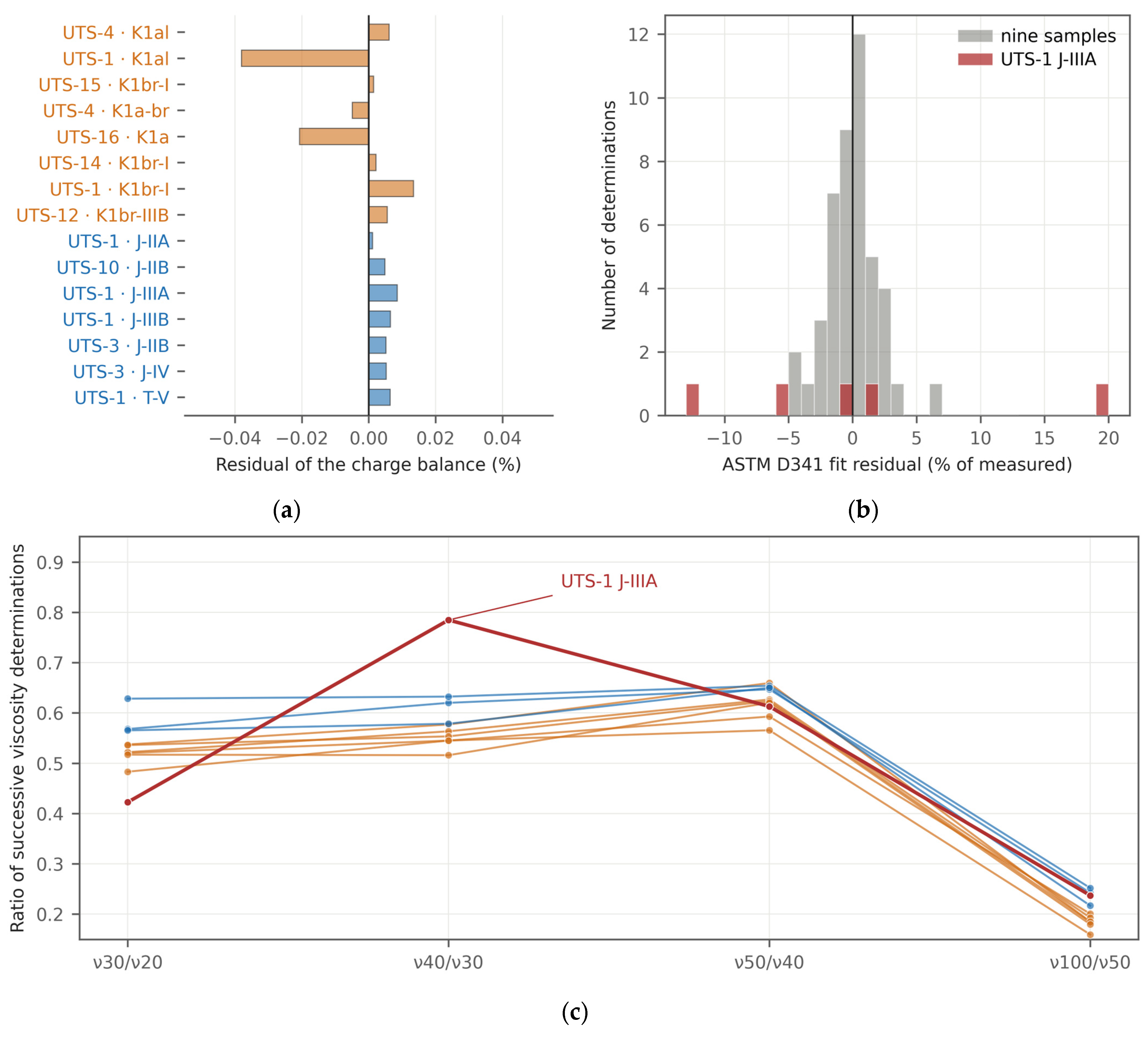
Figure A2.
Regression diagnostics and bootstrap slope distributions for the two pooled relations of Section 4.4: (a–d) log10 viscosity on saturates, (e–h) log10 viscosity on total sulfur. Panels are, in order, residuals against fitted value, normal quantile plot, leverage against standardised residual, and the bootstrap slope distribution with its percentile interval. Orange is Lower Cretaceous and blue Jurassic. Over 20,000 resamples the slope changes sign in 0.07% of the saturate resamples and in none of the sulfur resamples.
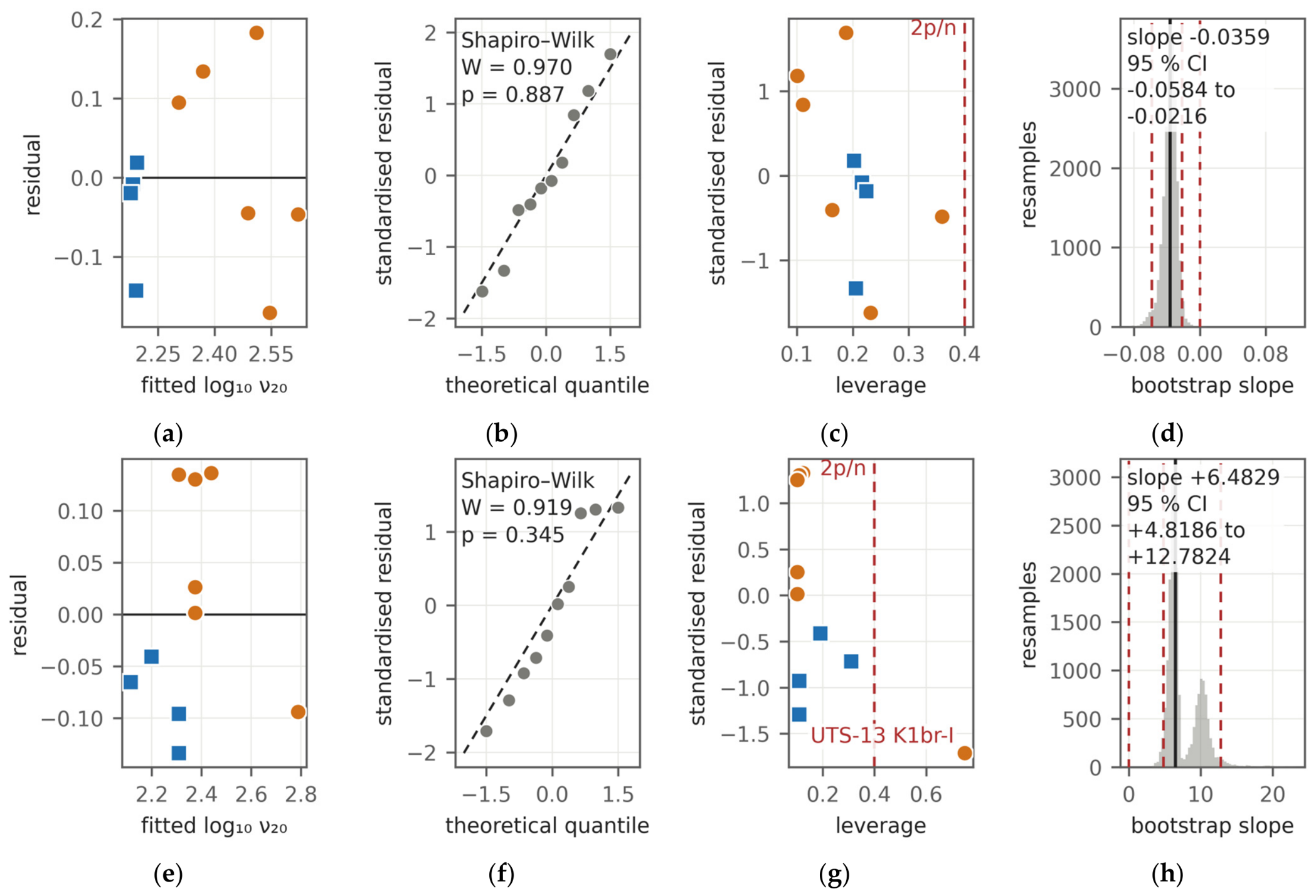
Figure A3.
Spearman rank correlation matrices for the oil properties: (a) All ten samples, (b) the six Cretaceous samples, and (c) the four Jurassic samples. Cells reaching an absolute coefficient of 0.75 are outlined and counted beneath each panel. These are rank coefficients over every pair of properties; they are not the quantity tabulated in Table A6, which gives Pearson coefficients of one response, log10 of the kinematic viscosity at 20 °C, against ten predictors. The within-group matrices are not sparser than the pooled one, but with six and four observations almost none of their coefficients is resolvable.
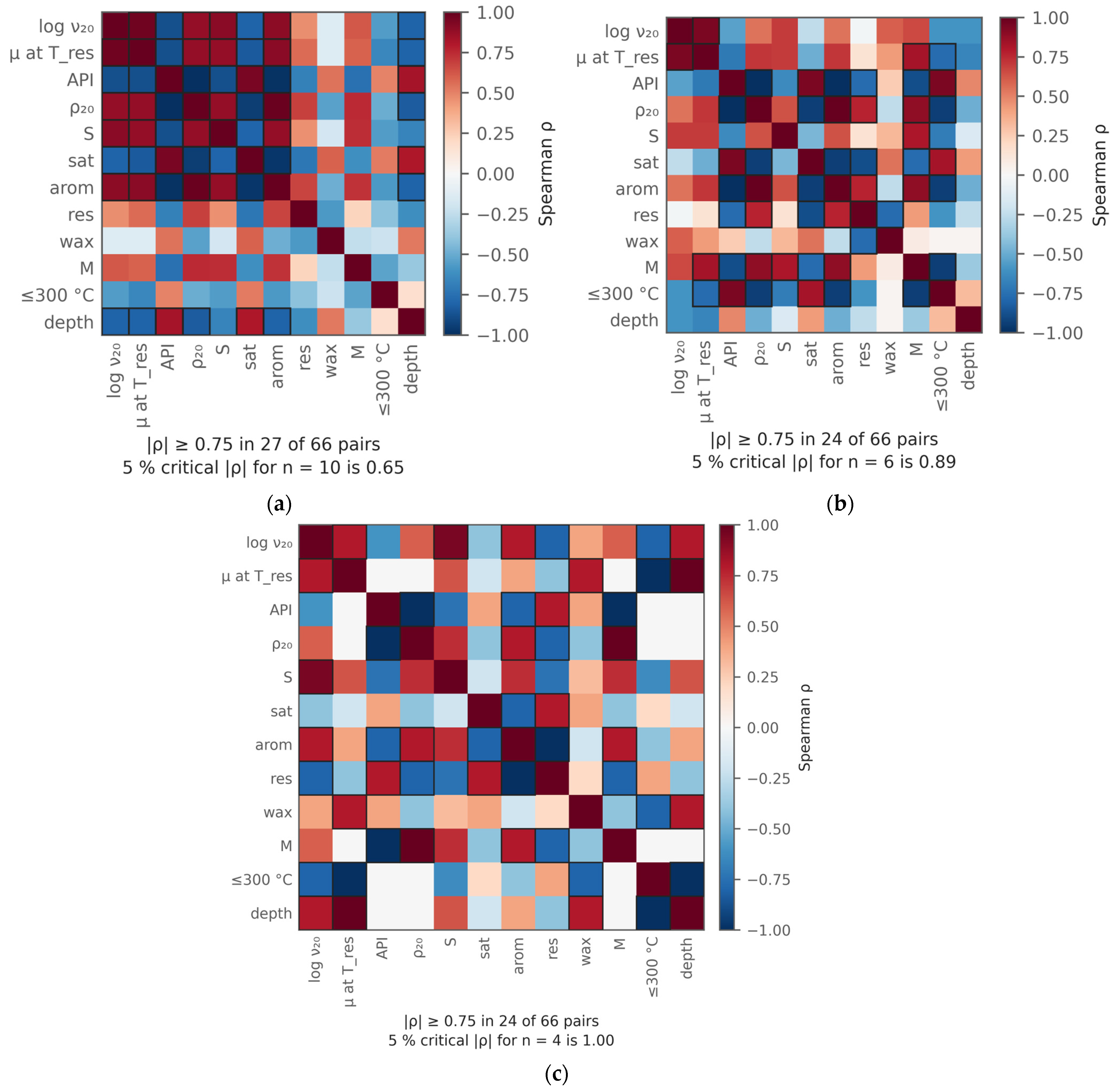
Figure A4.
Formation-water chemistry against depth: (a) Total dissolved solids, (b) sulfate relative to chloride, and (c) sodium relative to chloride. Symbols distinguish the Cretaceous reservoir waters, the two Albian aquifer samples, the Jurassic reservoir waters and the Triassic control; the legend is in panel (c). The grey band is the interval in which no oil was sampled, as in Figure 6a and Figure 9.
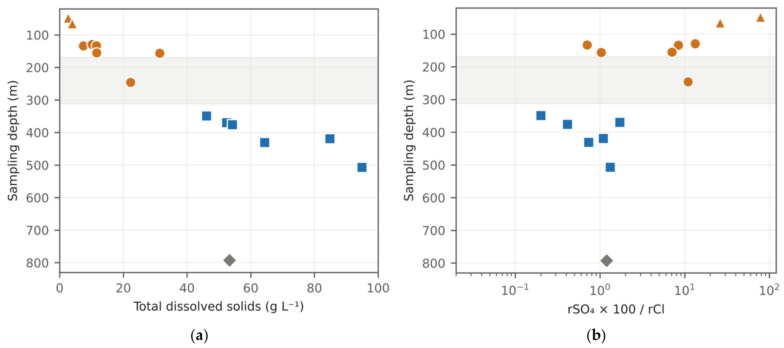
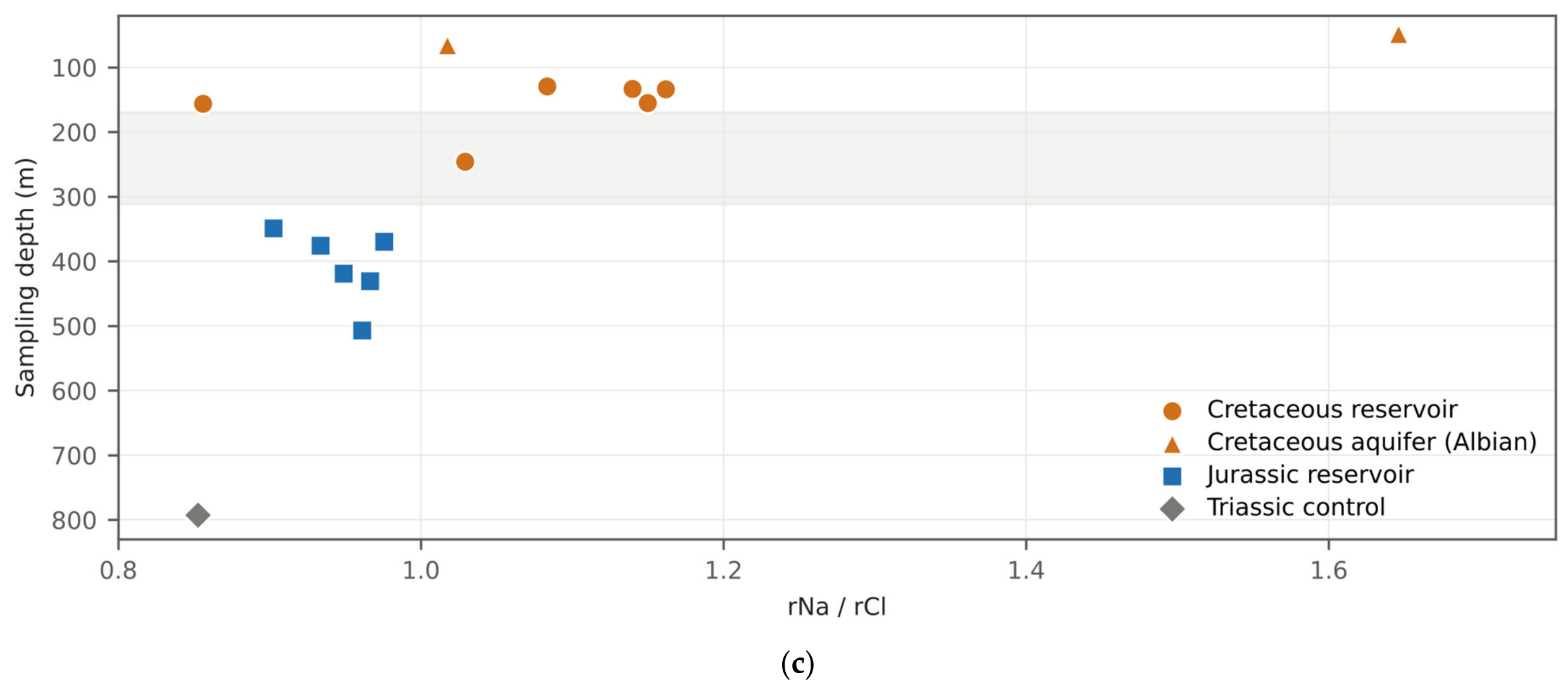
Figure A5.
Schoeller diagram of the fifteen formation-water analyses, concentrations in meq L−1. Reservoir waters of the two complexes, the two Albian aquifer samples and the Triassic control are distinguished by symbol. Sulfate and hydrogen carbonate depart strongly from the ratios that dilution would preserve, and the sodium-to-chloride ratio crosses unity between the complexes; sodium was obtained by difference, so its position is not an independent measurement.
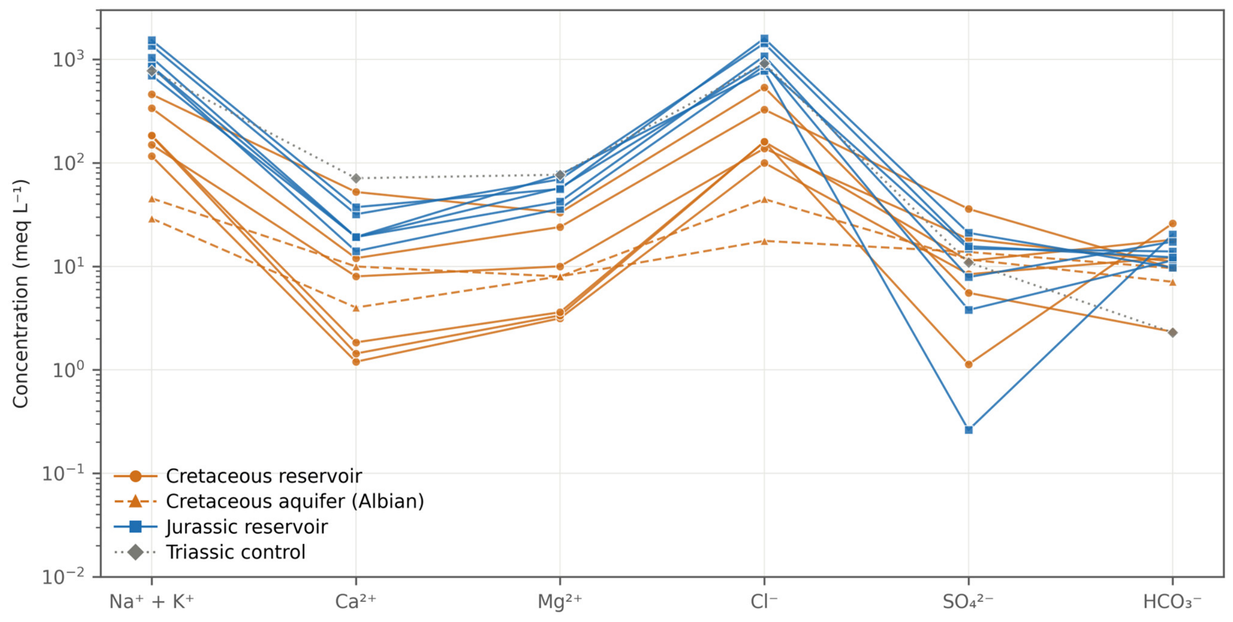
Figure A6.
Height of each oil sample above its own oil–water contact, for the nine samples whose pool has a mapped contact. (a) Height against modelled viscosity at reservoir temperature; the printed values are Pearson r with the exact permutation p in brackets, on nine and on six samples. (b) The same heights as bars, ordered by height. The Cretaceous samples sit well above their contacts and the Jurassic samples at them, which is the opposite of the geometry a simple sampling artefact would require.
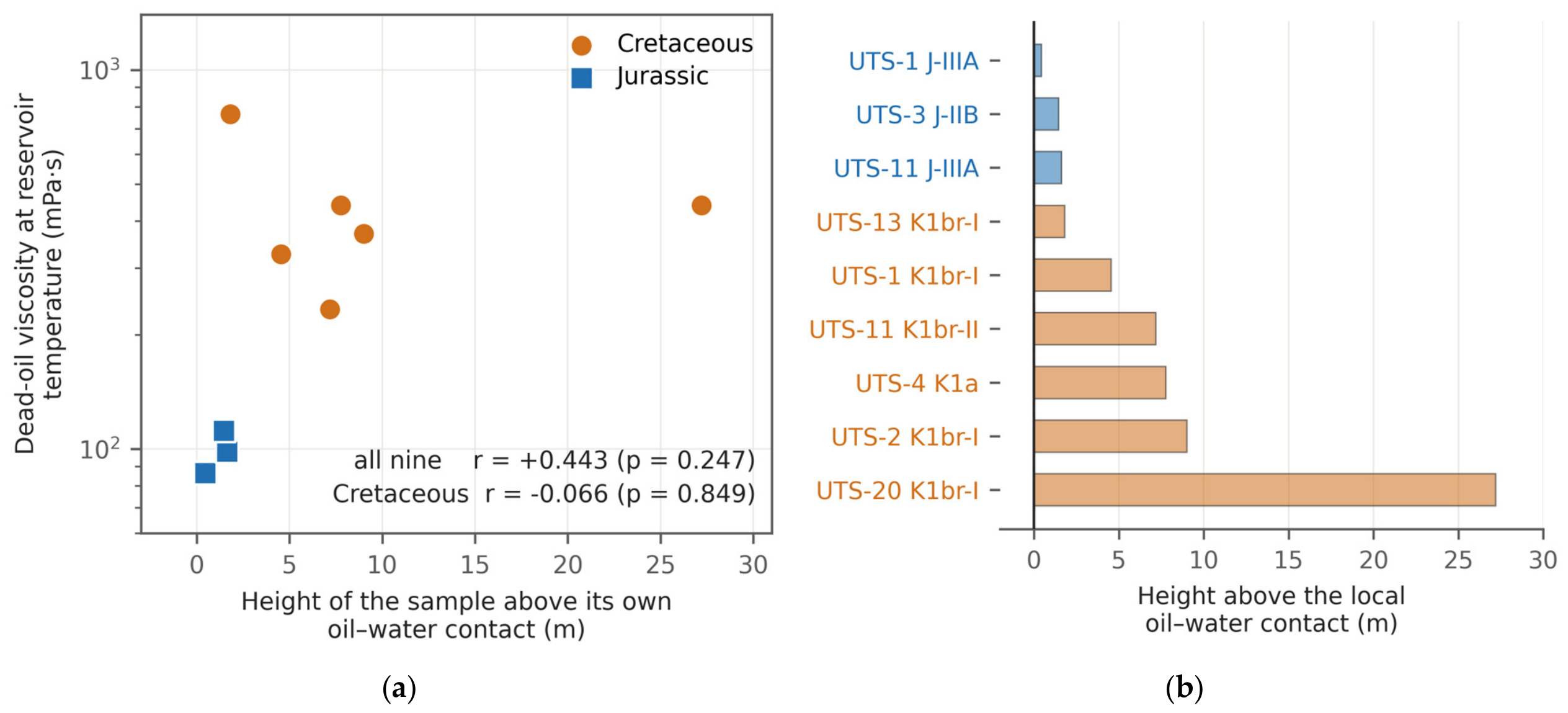
Figure A7.
Additional burial that would be required for the Cretaceous and Jurassic reservoirs to have reached a palaeopasteurisation threshold of about 80 °C, as a function of the assumed palaeogeothermal gradient and for an assumed surface temperature of 10 °C. The dashed line marks the gradient fitted to all eight bottom-hole temperatures (Section 4.6). No thermal effect of the salt is included in either direction.
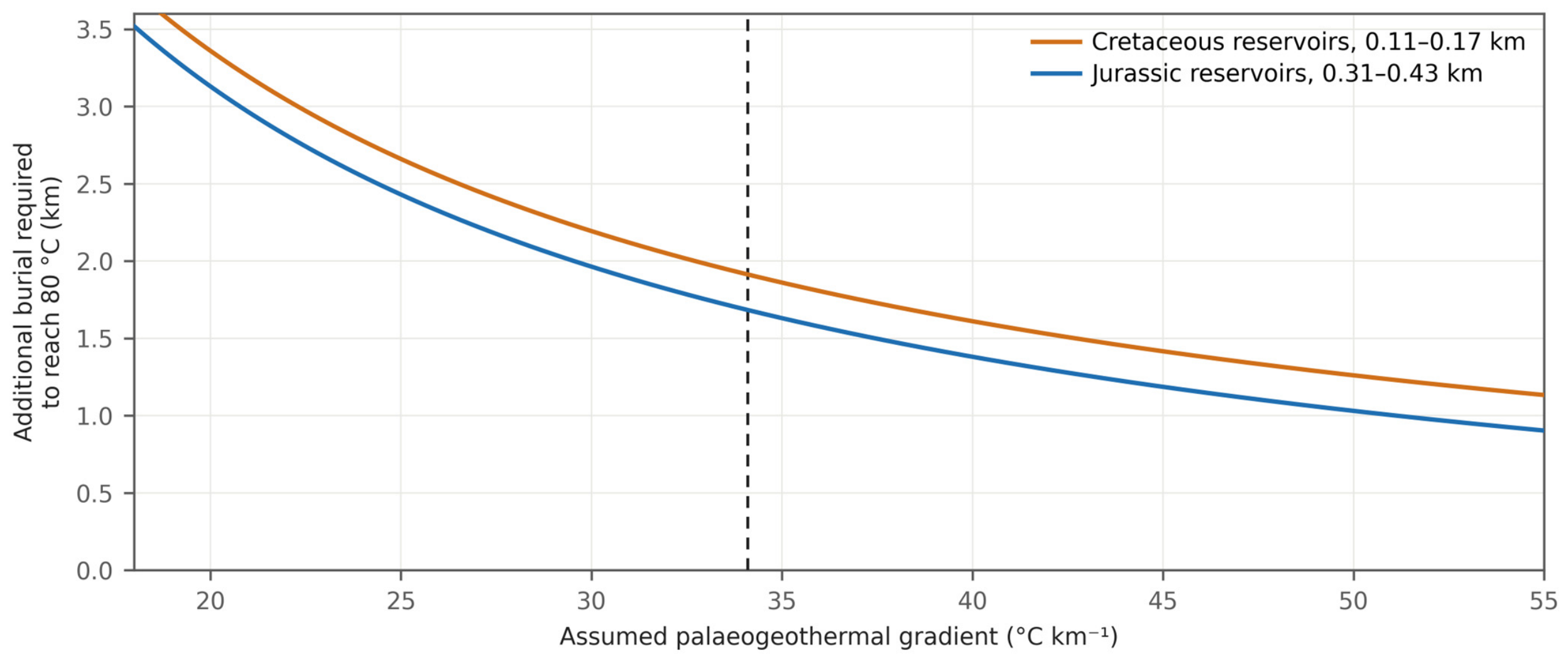
Figure A8.
Mixed-layer illite–smectite in the <2 µm clay fraction of the cored intervals against depth, from twenty determinations in UTS-2 and UTS-4 core. The mixed-layer phase is randomly interstratified (R0) with 20–30% illite layers. Crosses mark samples in which it was not detected; the deepest, at 350.5 m, is the only Jurassic sample.
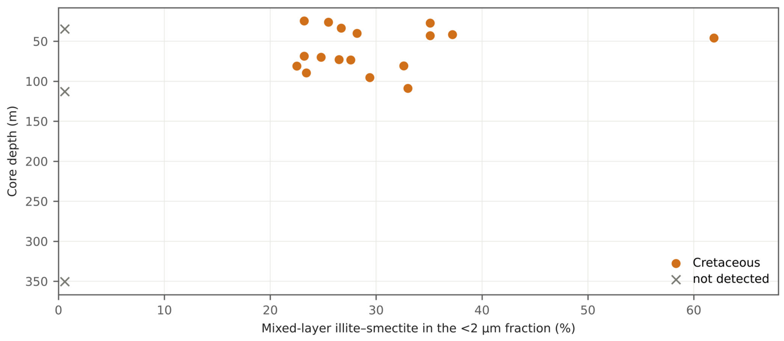
Figure A9.
Present-day temperature and pressure. (a) Bottom-hole temperature against depth, with the fit on all eight points, 3.41 ± 1.49 °C per 100 m, and the fit without the single deep point, 1.87 ± 7.15. The two probabilities printed in this panel, 0.001 and 0.53, are the parametric values for the regression slope and not permutation values; they are the only parametric probabilities in the figures. (b) Cook’s distance for that regression against the conventional threshold of 0.5. (c) Formation pressure against depth with two hydrostatic references; the sign of the comparison is set by the reference density.
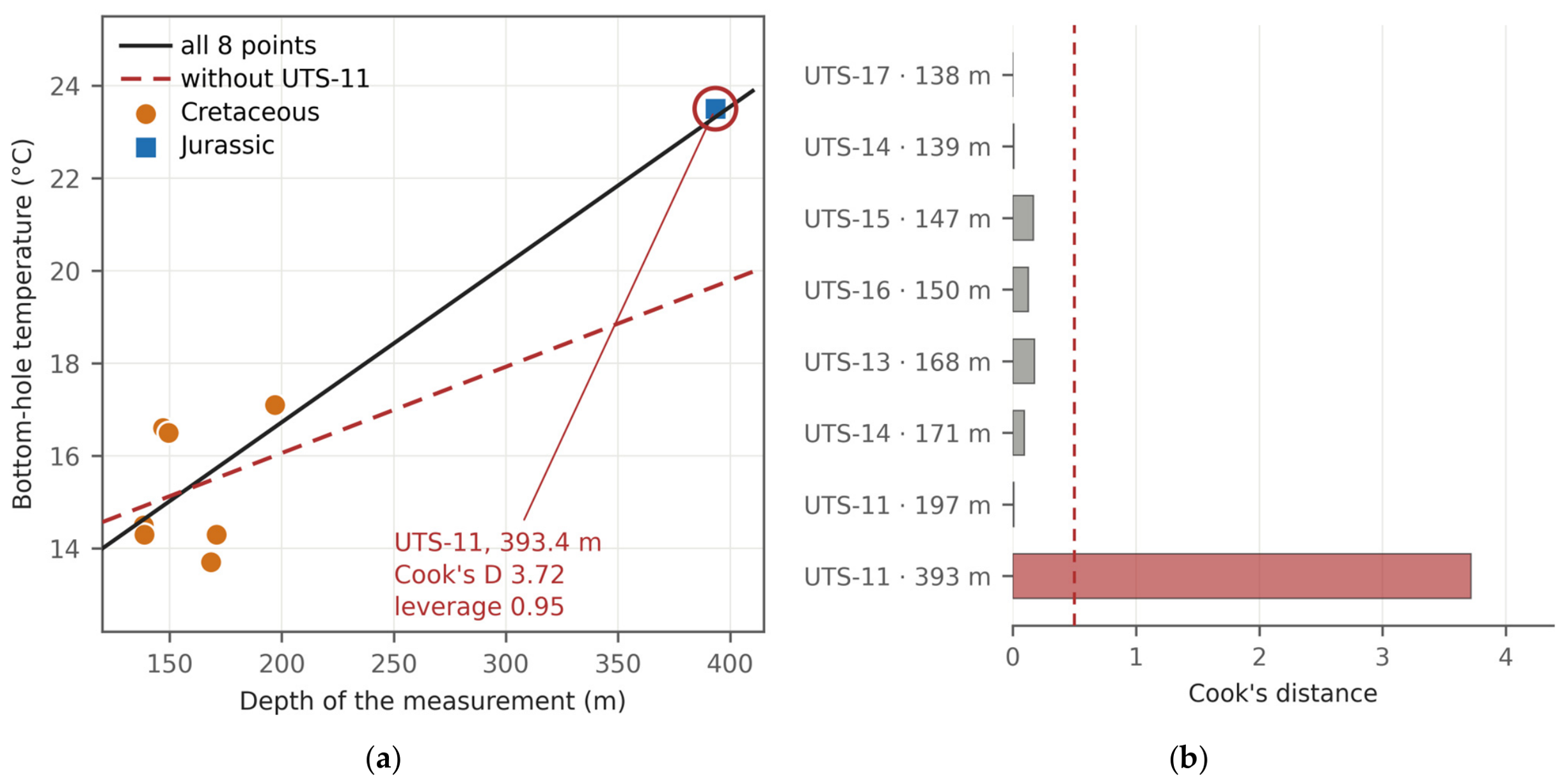
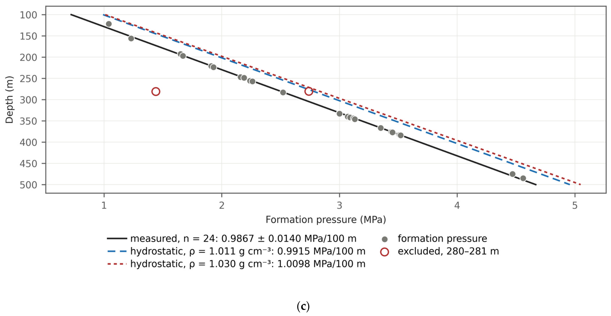
References
- Hudec, M.R.; Jackson, M.P.A. Terra infirma: Understanding salt tectonics. Earth-Sci. Rev. 2007, 82, 1–28. [Google Scholar] [CrossRef] [Scilit]
- Jackson, C.A.-L.; Duffy, O.B.; Fernandez, N.; Dooley, T.P.; Hudec, M.R.; Jackson, M.P.A.; Burg, G. The stratigraphic record of minibasin subsidence, Precaspian Basin, Kazakhstan. Basin Res. 2020, 32, 739–763. [Google Scholar] [CrossRef] [Scilit]
- Pichel, L.M.; Jackson, C.A.-L. Four-dimensional variability of composite halokinetic sequences. Basin Res. 2020, 32, 1277–1299. [Google Scholar] [CrossRef] [Scilit]
- Jackson, M.P.A.; Hudec, M.R. Salt Tectonics: Principles and Practice; Cambridge University Press: Cambridge, UK, 2017. [Google Scholar] [CrossRef] [Scilit]
- Zhou, H.; Li, W.; Zhang, B.; Liu, J.; Deng, S.; Zhang, S.; Shan, X.; Zhang, J.; Wang, X.; Jiang, H. Formation and evolution of intraplatform basin from the late Sinian to early Cambrian in Sichuan Basin, China. Pet. Res. 2017, 2, 41–53. [Google Scholar] [CrossRef] [Scilit]
- Zhemchuzhnikov, V.; Akhmetzhanov, A.; Ibrashev, K.; Akhmetzhanova, G. The geotectonic peculiarities of the North Caspian Permian salt-bearing basins (Kazakhstan). Geosciences 2024, 14, 23. [Google Scholar] [CrossRef] [Scilit]
- Volozh, Y.; Talbot, C.; Ismail-Zadeh, A. Salt structures and hydrocarbons in the Pricaspian basin. AAPG Bull. 2003, 87, 313–334. [Google Scholar] [CrossRef] [Scilit]
- Ulmishek, G.F. Petroleum Geology and Resources of the North Caspian Basin, Kazakhstan and Russia; U.S. Geological Survey Bulletin; U.S. Geological Survey: Washington, DC, USA, 2001; Volume 2201-B, 25p.
- Okere, D.; Toothill, S. New insights into hydrocarbon plays in the Caspian Sea, Kazakhstan. Pet. Geosci. 2012, 18, 253–268. [Google Scholar] [CrossRef] [Scilit]
- Akhmetzhanov, A.; Uvakova, S.; Ibrashev, K.; Akhmetzhanova, G.; Zhemchuzhnikov, V. The supra-salt sedimentary sequence of the North Caspian Depression: Stratigraphy and sedimentary history. Geosciences 2025, 15, 143. [Google Scholar] [CrossRef] [Scilit]
- Akhmetzhanov, A.; Zholtayev, G.; Djeddou, A.; Akhmetzhanova, G.; Oraz, B. Post-salt trapping mechanism of south-east Pre-Caspian and its application to petroleum exploration. J. Pet. Explor. Prod. Technol. 2020, 10, 2645–2653. [Google Scholar] [CrossRef] [Scilit]
- Zholdybayeva, A.; Syzdykov, A.; Pourafshary, P.; Ismailova, J.; Delikesheva, D. Importance of clay swelling on the efficacy of cyclic steam stimulation in the East Moldabek formation in Kazakhstan. Energies 2024, 17, 5078. [Google Scholar] [CrossRef] [Scilit]
- Soltanbekova, K.; Ramazanova, G.; Zhapbasbayev, U.; Kuatov, Z. Filtration experiments for assessing EOR efficiency in high-viscosity oil reservoirs: A case study of the East Moldabek field, Kazakhstan. Processes 2025, 13, 1069. [Google Scholar] [CrossRef] [Scilit]
- Head, I.M.; Jones, D.M.; Larter, S.R. Biological activity in the deep subsurface and the origin of heavy oil. Nature 2003, 426, 344–352. [Google Scholar] [CrossRef] [Scilit]
- Aitken, C.M.; Jones, D.M.; Larter, S.R. Anaerobic hydrocarbon biodegradation in deep subsurface oil reservoirs. Nature 2004, 431, 291–294. [Google Scholar] [CrossRef] [Scilit]
- Larter, S.; Wilhelms, A.; Head, I.; Koopmans, M.; Aplin, A.; di Primio, R.; Zwach, C.; Erdmann, M.; Telnaes, N. The controls on the composition of biodegraded oils in the deep subsurface—Part 1: Biodegradation rates in petroleum reservoirs. Org. Geochem. 2003, 34, 601–613. [Google Scholar] [CrossRef] [Scilit]
- Larter, S.; Huang, H.; Adams, J.; Bennett, B.; Jokanola, O.; Oldenburg, T.; Jones, M.; Head, I.; Riediger, C.; Fowler, M. The controls on the composition of biodegraded oils in the deep subsurface: Part II—Geological controls on subsurface biodegradation fluxes and constraints on reservoir-fluid property prediction. AAPG Bull. 2006, 90, 921–938. [Google Scholar] [CrossRef] [Scilit]
- Oldenburg, T.B.P.; Larter, S.R.; Huang, H. Nutrient supply during subsurface oil biodegradation—Availability of petroleum nitrogen as a nutrient source for subsurface microbial activity. Energy Fuels 2006, 20, 2079–2082. [Google Scholar] [CrossRef] [Scilit]
- Wilhelms, A.; Larter, S.R.; Head, I.; Farrimond, P.; di-Primio, R.; Zwach, C. Biodegradation of oil in uplifted basins prevented by deep-burial sterilisation. Nature 2001, 411, 1034–1037. [Google Scholar] [CrossRef] [Scilit]
- Fathepure, B.Z. Recent studies in microbial degradation of petroleum hydrocarbons in hypersaline environments. Front. Microbiol. 2014, 5, 173. [Google Scholar] [CrossRef] [Scilit]
- Martins, L.F.; Peixoto, R.S. Biodegradation of petroleum hydrocarbons in hypersaline environments. Braz. J. Microbiol. 2012, 43, 865–872. [Google Scholar] [CrossRef] [Scilit]
- Lafargue, E.; Barker, C. Effect of water washing on crude oil compositions. AAPG Bull. 1988, 72, 263–276. [Google Scholar] [CrossRef] [Scilit]
- Peters, K.E.; Moldowan, J.M. The Biomarker Guide: Interpreting Molecular Fossils in Petroleum and Ancient Sediments; Prentice Hall: Englewood Cliffs, NJ, USA, 1993; 363p. [Google Scholar]
- Larter, S.; Huang, H.; Adams, J.; Bennett, B.; Snowdon, L.R. A practical biodegradation scale for use in reservoir geochemical studies of biodegraded oils. Org. Geochem. 2012, 45, 66–76. [Google Scholar] [CrossRef] [Scilit]
- Adams, J.J.; Larter, S.R.; Bennett, B.; Huang, H.; Westrich, J.; van Kruisdijk, C. The dynamic interplay of oil mixing, charge timing, and biodegradation in forming the Alberta oil sands. AAPG Stud. Geol. 2013, 64, 23–102. [Google Scholar] [CrossRef] [Scilit]
- Cesar, J.; Ardakani, O.H.; Watt, E.; Song, Y.; Kingston, A.; Ahad, J.M.E. Paleo-biodegradation and hydrocarbon mixing in a major hybrid petroleum reservoir. Sci. Rep. 2023, 13, 4357. [Google Scholar] [CrossRef] [Scilit]
- O’Brien, J.J.; Lerche, I. The influence of salt domes on paleotemperature distributions. Geophysics 1984, 49, 2032–2043. [Google Scholar] [CrossRef] [Scilit]
- Vizgirda, J.; O’Brien, J.J.; Lerche, I. Thermal anomalies on the flanks of a salt dome. Geothermics 1985, 14, 553–565. [Google Scholar] [CrossRef] [Scilit]
- Jensen, P.K. Analysis of the temperature field around salt diapirs. Geothermics 1990, 19, 273–283. [Google Scholar] [CrossRef] [Scilit]
- Petersen, K.; Lerche, I. Quantification of thermal anomalies in sediments around salt structures. Geothermics 1995, 24, 253–268. [Google Scholar] [CrossRef] [Scilit]
- Mello, U.T.; Karner, G.D.; Anderson, R.N. Role of salt in restraining the maturation of subsalt source rocks. Mar. Pet. Geol. 1995, 12, 697–716. [Google Scholar] [CrossRef] [Scilit]
- Cedeno, A.; Rojo, L.A.; Cardozo, N.; Centeno, L.; Escalona, A. The impact of salt tectonics on the thermal evolution and the petroleum system of confined rift basins: Insights from basin modeling of the Nordkapp Basin, Norwegian Barents Sea. Geosciences 2019, 9, 316. [Google Scholar] [CrossRef] [Scilit]
- Canova, D.P.; Fischer, M.P.; Jayne, R.S.; Pollyea, R.M. Advective heat transport and the salt chimney effect: A numerical analysis. Geofluids 2018, 2018, 2378710. [Google Scholar] [CrossRef] [Scilit]
- Ranganathan, V.; Hanor, J.S. Density-driven groundwater flow near salt domes. Chem. Geol. 1988, 74, 173–188. [Google Scholar] [CrossRef] [Scilit]
- Evans, D.G.; Nunn, J.A.; Hanor, J.S. Mechanisms driving groundwater flow near salt domes. Geophys. Res. Lett. 1991, 18, 927–930. [Google Scholar] [CrossRef] [Scilit]
- Ma, Y.Z. Simpson’s paradox in natural resource evaluation. Math. Geosci. 2009, 41, 193–213. [Google Scholar] [CrossRef] [Scilit]
- Yeginbayeva, A.Y.; Saparov, K.T.; Abdullina, A.G.; Shakhantayeva, Z.R. Geographical problems of unification of the toponymic system of Kazakhstan. Geogr. Water Resour. 2024, 2, 134–142. [Google Scholar] [CrossRef] [Scilit]
- Barde, J.-P.; Chamberlain, P.; Galavazi, M.; Gralla, P.; Harwijanto, J.; Marsky, J.; van den Belt, F. Sedimentation during halokinesis: Permo-Triassic reservoirs of the Saigak Field, Precaspian Basin, Kazakhstan. Pet. Geosci. 2002, 8, 177–187. [Google Scholar] [CrossRef] [Scilit]
- Nuraliev, B.B.; Turkov, O.S.; Shilina, V.A.; Averyanova, S.G.; Amelichkina, M.I.; Osipova, L.A.; Gracheva, A.V.; Ospanova, K.S. Generalisation of Seismic and Gravity Data on the South of the Precaspian Depression for Compiling Summary Structural Maps of the Supra-Salt Deposits and the Top of the Salt. 1976; Unpublished Report. (In Russian)
- GOST 33-2000; Petroleum Products. Transparent and Opaque Liquids. Determination of Kinematic Viscosity and Calculation of Dynamic Viscosity. IPK Izdatel’stvo Standartov: Moscow, Russia, 2000.
- ST RK ASTM D445-2011; Standard Test Method for Kinematic Viscosity of Transparent and Opaque Liquids (and Calculation of Dynamic Viscosity). Committee for Technical Regulation and Metrology: Astana, Kazakhstan, 2011.
- GOST 3900-85; Petroleum and Petroleum Products. Methods for Determination of Density. Izdatel’stvo Standartov: Moscow, Russia, 1985.
- GOST R 51947-2002; Petroleum and Petroleum Products. Determination of Sulphur by Method of Energy-Dispersive X-ray Fluorescence Spectrometry. IPK Izdatel’stvo Standartov: Moscow, Russia, 2002.
- ASTM D4294-98; Standard Test Method for Sulfur in Petroleum and Petroleum Products by Energy-Dispersive X-ray Fluorescence Spectrometry. American Society for Testing and Materials: West Conshohocken, PA, USA, 1998.
- GOST 1437-75; Dark Petroleum Products. Accelerated Method for Determination of Sulphur. Izdatel’stvo Standartov: Moscow, Russia, 1975.
- GOST 11244-76; Petroleum. Method for the Determination of Distillation and Residue Oils Potential Content. Izdatel’stvo Standartov: Moscow, Russia, 1976.
- GOST 11851-85; Petroleum. Method of Paraffin Determination. Izdatel’stvo Standartov: Moscow, Russia, 1985.
- GOST 2177-99; Petroleum Products. Methods for Determination of Distillation Characteristics. IPK Izdatel’stvo Standartov: Moscow, Russia, 1999.
- GOST 20287-91; Petroleum Products. Methods of Test for Flow Point and Pour Point. Izdatel’stvo Standartov: Moscow, Russia, 1991.
- GOST 6356-75; Petroleum Products. Method of Test for Flash Point by Closed Cup. Izdatel’stvo Standartov: Moscow, Russia, 1975.
- GOST 4333-87; Petroleum Products. Methods for Determination of Flash and Ignition Points in Open Crucible. Izdatel’stvo Standartov: Moscow, Russia, 1987.
- ASTM D341-20e1; ASTM International Standard Practice for Viscosity-Temperature Equations and Charts for Liquid Petroleum or Hydrocarbon Products. ASTM International: West Conshohocken, PA, USA, 2020. [Google Scholar] [CrossRef] [Scilit]
- Beggs, H.D.; Robinson, J.R. Estimating the viscosity of crude oil systems. J. Pet. Technol. 1975, 27, 1140–1141. [Google Scholar] [CrossRef] [Scilit]
- ASTM D1250-19e1; ASTM International Standard Guide for the Use of the Joint API and ASTM Adjunct for Temperature and Pressure Volume Correction Factors for Generalized Crude Oils, Refined Products, and Lubricating Oils: API MPMS Chapter 11.1. ASTM International: West Conshohocken, PA, USA, 2019. [Google Scholar] [CrossRef] [Scilit]
- Meyer, R.F.; Attanasi, E.D. Heavy Oil and Natural Bitumen—Strategic Petroleum Resources; U.S. Geological Survey Fact Sheet; 70-03; U.S. Geological Survey: Washington, DC, USA, 2003.
- Zhang, W.; Wu, J.; Li, S.; Zhang, Y.; Zhao, S.; Shi, Q. Classification method of heavy oil based on chemical composition and bulk properties. Energies 2024, 17, 3733. [Google Scholar] [CrossRef] [Scilit]
- Sulin, V.A. Hydrogeology of Oil Fields; Gostoptekhizdat: Moscow, Russia, 1946. (In Russian) [Google Scholar]
- Hem, J.D. Study and Interpretation of the Chemical Characteristics of Natural Water, 3rd ed.; U.S. Geological Survey Water-Supply Paper; U.S. Geological Survey: Washington, DC, USA, 1985; Volume 2254, 263p.
- Ernst, M.D. Permutation methods: A basis for exact inference. Stat. Sci. 2004, 19, 676–685. [Google Scholar] [CrossRef] [Scilit]
- Benjamini, Y.; Hochberg, Y. Controlling the false discovery rate: A practical and powerful approach to multiple testing. J. R. Stat. Soc. Ser. B 1995, 57, 289–300. [Google Scholar] [CrossRef] [Scilit]
- Welch, B.L. The generalization of Student’s problem when several different population variances are involved. Biometrika 1947, 34, 28–35. [Google Scholar] [CrossRef] [Scilit]
- Mann, H.B.; Whitney, D.R. On a test of whether one of two random variables is stochastically larger than the other. Ann. Math. Stat. 1947, 18, 50–60. [Google Scholar] [CrossRef] [Scilit]
- Hedges, L.V. Distribution theory for Glass’s estimator of effect size and related estimators. J. Educ. Stat. 1981, 6, 107–128. [Google Scholar] [CrossRef] [Scilit]
- Cliff, N. Dominance statistics: Ordinal analyses to answer ordinal questions. Psychol. Bull. 1993, 114, 494–509. [Google Scholar] [CrossRef]
- Stone, M. Cross-validatory choice and assessment of statistical predictions. J. R. Stat. Soc. Ser. B 1974, 36, 111–133. [Google Scholar] [CrossRef] [Scilit]
- Aitchison, J. The statistical analysis of compositional data. J. R. Stat. Soc. Ser. B 1982, 44, 139–160. [Google Scholar] [CrossRef] [Scilit]
- Cook, R.D. Detection of influential observation in linear regression. Technometrics 1977, 19, 15–18. [Google Scholar] [CrossRef] [Scilit]
- Jones, D.M.; Head, I.M.; Gray, N.D.; Adams, J.J.; Rowan, A.K.; Aitken, C.M.; Bennett, B.; Huang, H.; Brown, A.; Bowler, B.F.J.; et al. Crude-oil biodegradation via methanogenesis in subsurface petroleum reservoirs. Nature 2008, 451, 176–180. [Google Scholar] [CrossRef] [Scilit]
- Pairazian, V.V. A review of the petroleum geochemistry of the Precaspian Basin. Pet. Geosci. 1999, 5, 361–369. [Google Scholar] [CrossRef] [Scilit]
- Zhanserkeyeva, A.A.; Kassenov, A.K. Prospect evaluation based on integrated petroleum system analysis: Block E case study, south-eastern edge of Precaspian Basin (Kazakhstan). J. Pet. Explor. Prod. Technol. 2022, 12, 2625–2642. [Google Scholar] [CrossRef] [Scilit]
- Zhanserkeyeva, A.A. Source rocks evaluation of the Late Devonian succession at Koblandy-3 well, the Northern Precaspian Basin. Geol. Subsoil Prot. 2024, 1, 72–76. [Google Scholar]
- Gürgey, K. An attempt to recognise oil populations and potential source rock types in Paleozoic sub- and Mesozoic–Cenozoic supra-salt strata in the southern margin of the Pre-Caspian Basin, Kazakhstan Republic. Org. Geochem. 2002, 33, 723–741. [Google Scholar] [CrossRef] [Scilit]
- Freeman, J.T. The use of bromide and chloride mass ratios to differentiate salt-dissolution and formation brines in shallow groundwaters of the Western Canadian Sedimentary Basin. Hydrogeol. J. 2007, 15, 1377–1385. [Google Scholar] [CrossRef] [Scilit]
- Xie, Y.; Liu, Y.; Han, J.; Huang, C.; Zhu, L.; Lou, Z.; Jin, A.; Zhu, R. Chemical characteristics of Ordovician formation water and its relationship with hydrocarbon distribution in Shunbei and adjacent regions, Tarim Basin, NW China. Water 2026, 18, 714. [Google Scholar] [CrossRef] [Scilit]
- Head, I.M.; Gray, N.D.; Larter, S.R. Life in the slow lane; biogeochemistry of biodegraded petroleum containing reservoirs and implications for energy recovery and carbon management. Front. Microbiol. 2014, 5, 566. [Google Scholar] [CrossRef] [Scilit]
- Ismail-Zadeh, A.; Wilhelm, H.; Volozh, Y.; Tinakin, O. The Astrakhan Arch of the Pricaspian basin: Geothermal analysis and modelling. Basin Res. 2010, 22, 751–764. [Google Scholar] [CrossRef] [Scilit]
- Srodon, J. Nature of mixed-layer clays and mechanisms of their formation and alteration. Annu. Rev. Earth Planet. Sci. 1999, 27, 19–53. [Google Scholar] [CrossRef] [Scilit]
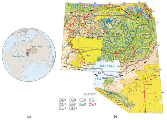
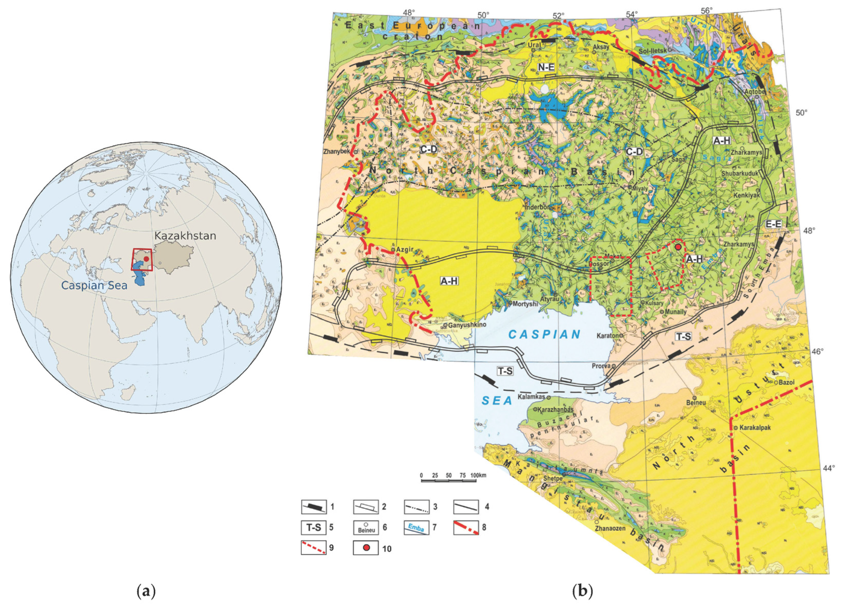
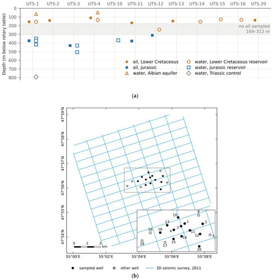
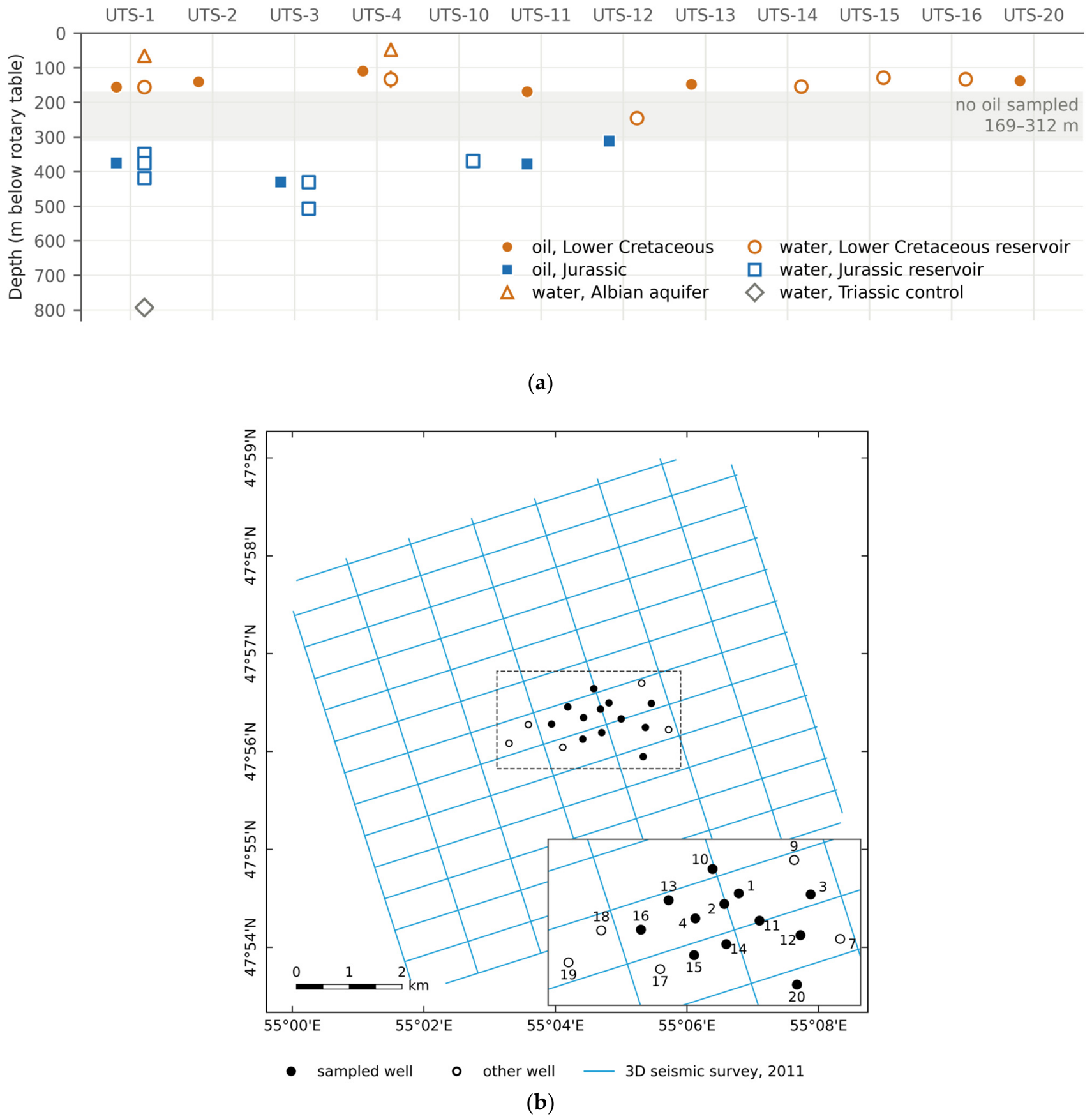
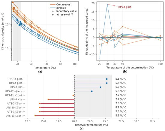
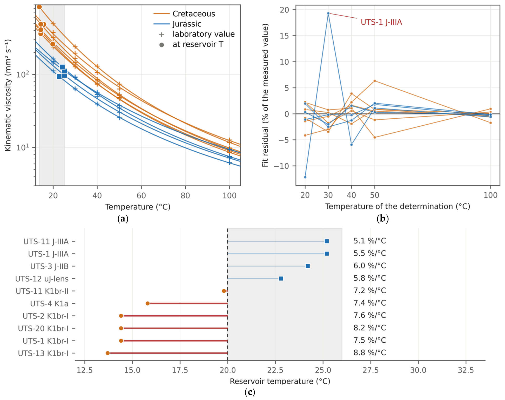
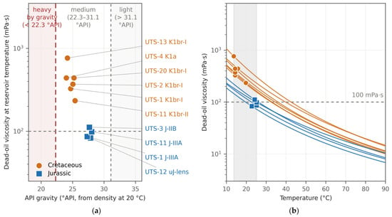
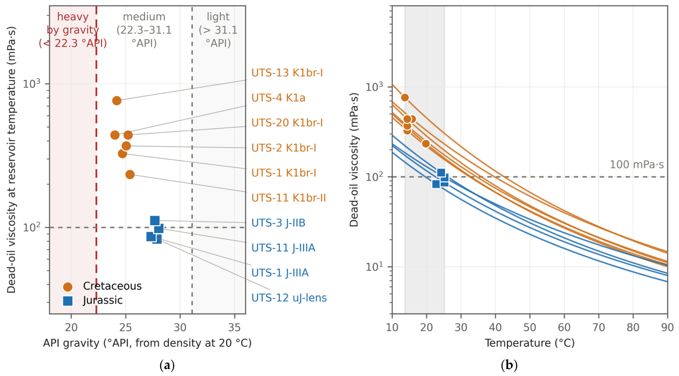
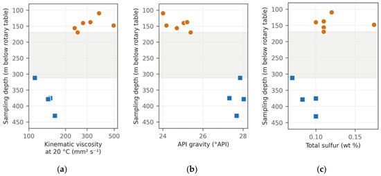
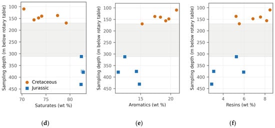
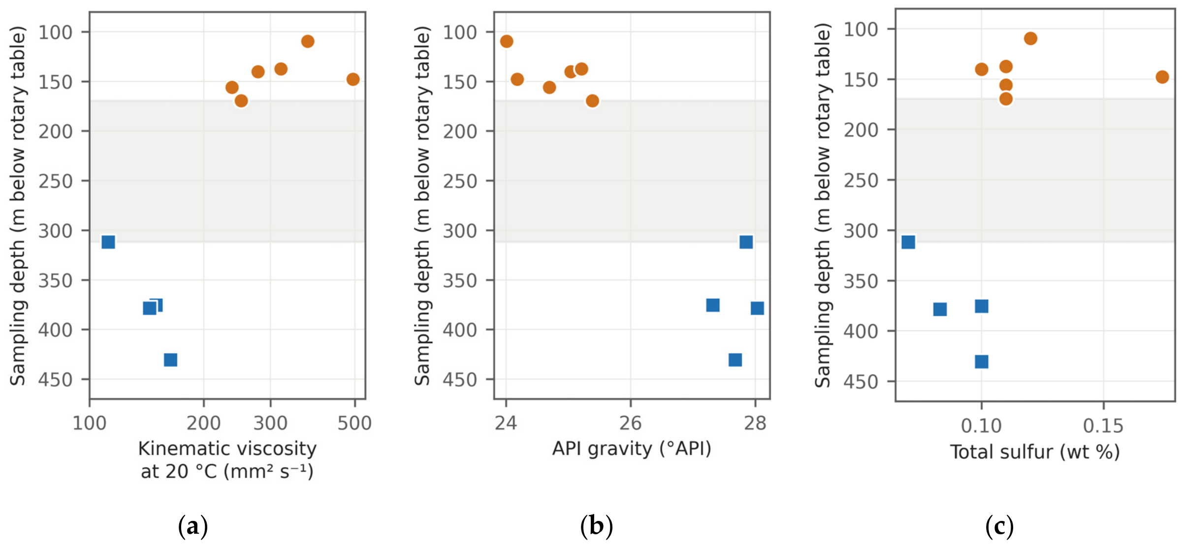
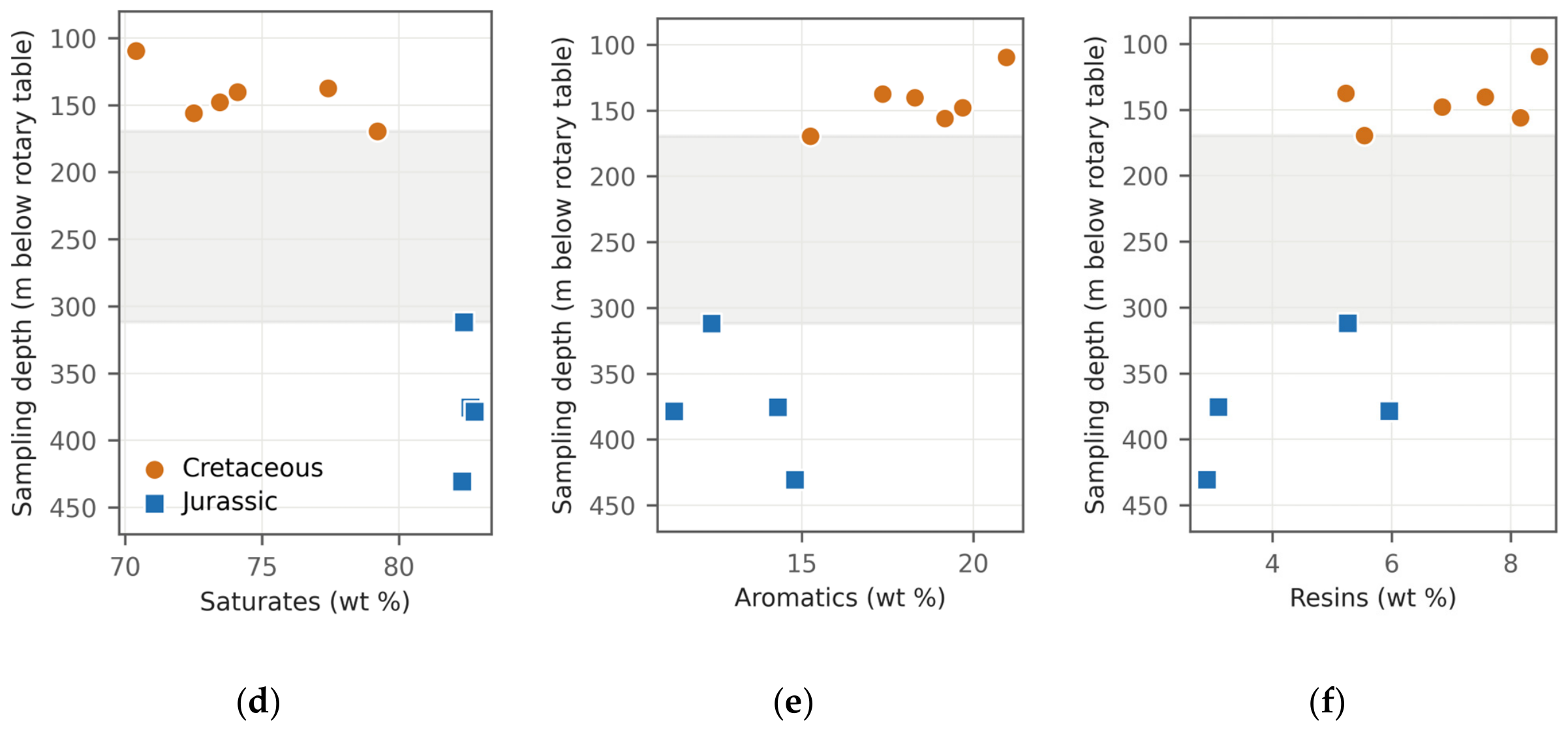
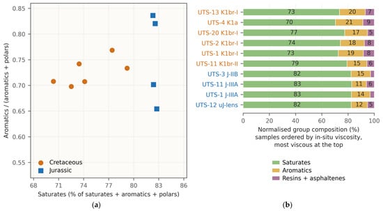
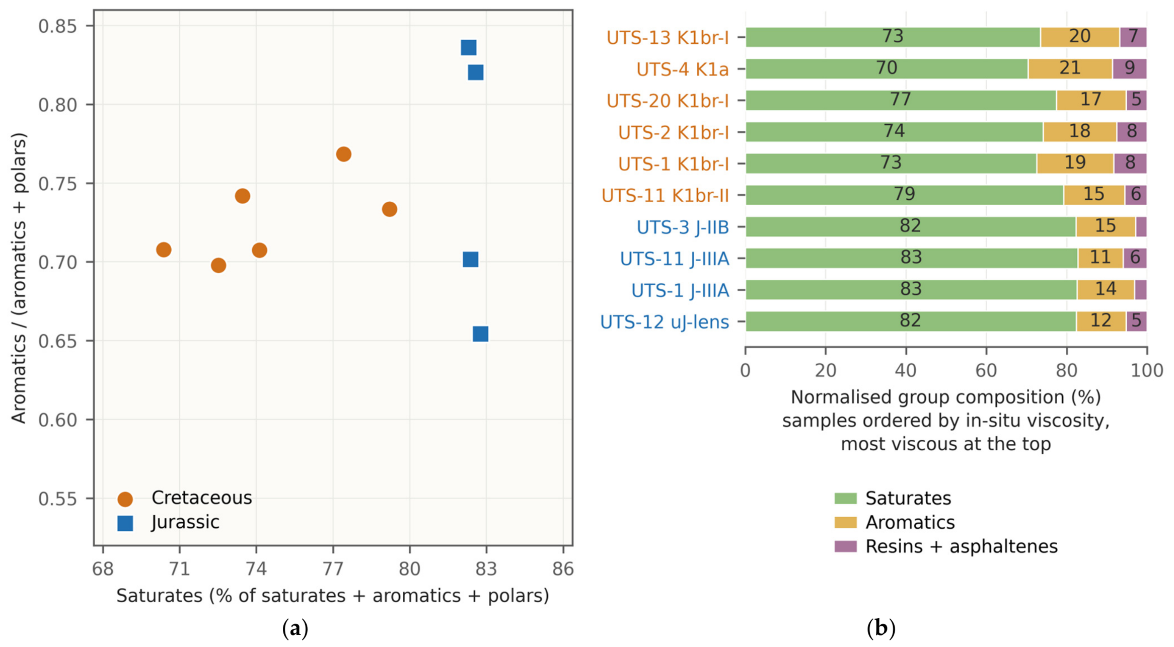
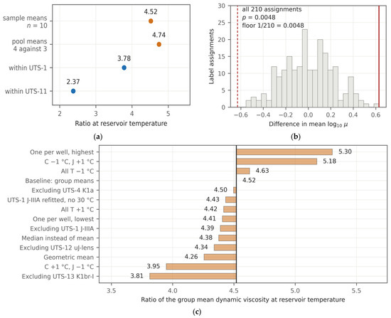
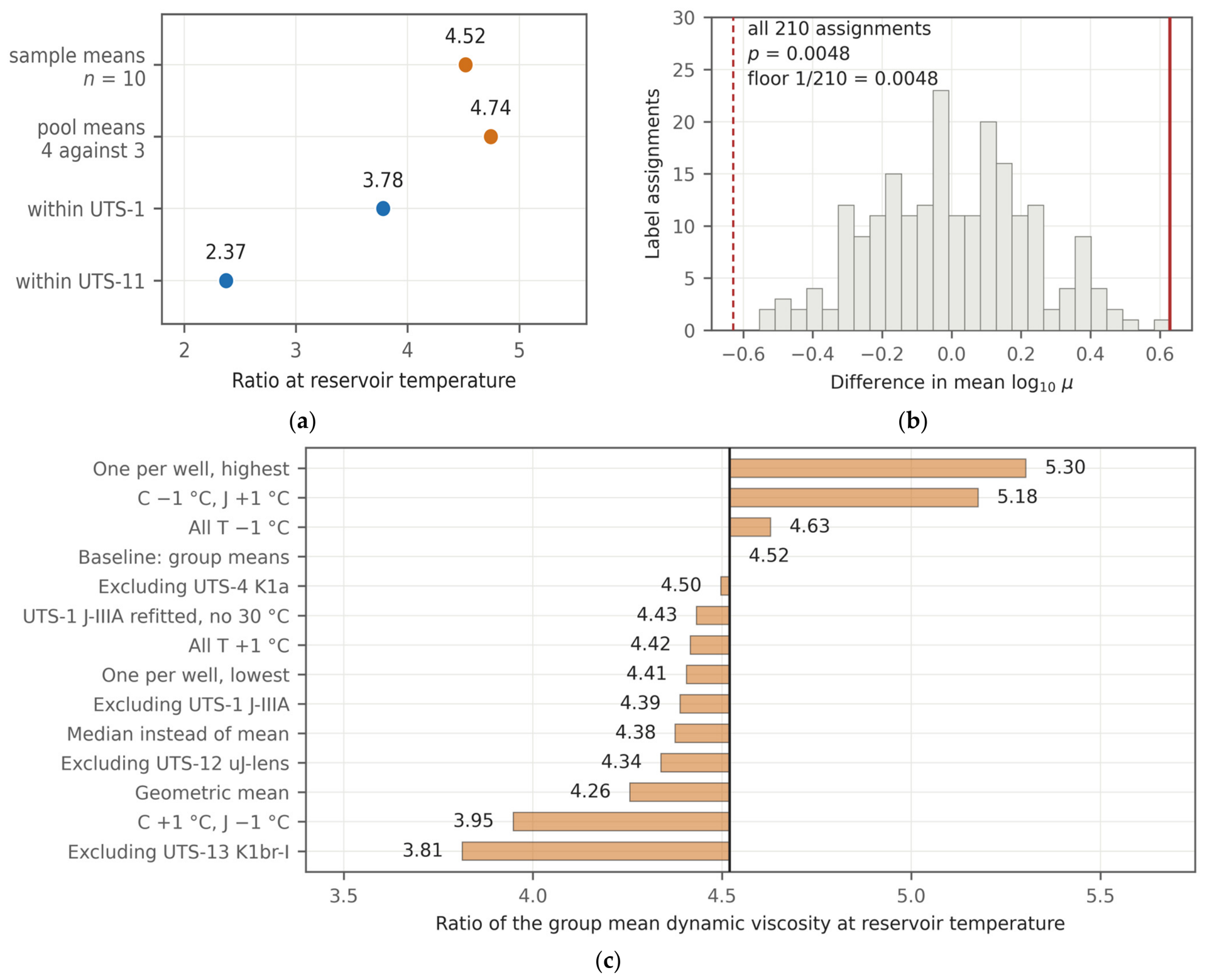
Disclaimer/Publisher’s Note: The statements, opinions and data contained in all publications are solely those of the individual author(s) and contributor(s) and not of MDPI and/or the editor(s). MDPI and/or the editor(s) disclaim responsibility for any injury to people or property resulting from any ideas, methods, instructions or products referred to in the content. |
© 2026 by the authors. Licensee MDPI, Basel, Switzerland. This article is an open access article distributed under the terms and conditions of the Creative Commons Attribution (CC BY) license.