Off-Policy Inverse Q-Learning Algorithm with Unobservable States

Abstract

To address the problem of an unknown performance index in discrete-time (DT) linear systems with unobservable states, this paper investigates the output-feedback inverse reinforcement learning (IRL) problem and proposes a data-driven output-feedback off-policy inverse Q-learning algorithm. The proposed method relies solely on input–output trajectory data from an expert system. It does not require a system-dynamics model or state information to identify the unknown cost function and learn an optimal control policy. First, for cases where the system dynamics and the target control gain are known, we propose a model-based method. Building on this foundation, we further develop a model-free method that does not require a system-dynamics model or state information. The proposed algorithm uses state reconstruction to transform the state-feedback Q-function equation into an input–output form. Simulations using an F-16 aircraft model demonstrate that the learner system can approximate the expert trajectories and effectively reconstruct the performance-index function.

1. Introduction

With the advancement of optimal control theory, it has become possible to design control strategies based on known system models and performance indexes [1]. However, precise models and performance indexes for real world systems are often difficult to obtain, which makes the direct application of traditional optimal-control methods challenging [2,3]. Reinforcement learning, as a significant advancement in this field, relaxes the requirements for system models and allows control strategies to be learned incrementally through interaction with the environment. Nevertheless, it also relies on a predefined and well-designed cost function. When the performance index cannot be clearly defined, both approaches face fundamental challenges.

To address this issue, inverse reinforcement learning (IRL) [4,5], also known as imitation learning, was proposed. It reconstructs the latent cost function from expert demonstration data. Unlike traditional reinforcement learning, IRL can infer the underlying objective function by observing the expert’s optimal behaviour [6,7,8]. However, most existing research focuses on state-feedback scenarios and typically assumes that the system state is fully observable. Only [9,10] address the issue of unobservable system states. Xue et al. [9] proposed an algorithm based on static output-feedback control for continuous-time systems under external disturbances. However, this method employs a double-loop iterative structure, requiring repeated updates of the control policy and cost function in both inner and outer loops, resulting in high computational complexity. In recent years, IRL has been extensively studied in random systems [11,12,13,14,15], dynamic systems [16,17,18,19], and trajectory emulation [20,21,22]. It has gradually been integrated with methods such as data-driven control [21] and inverse optimal control, forming a class of important tools capable of simultaneously explaining expert behaviour and recovering control laws.

Related advances in control and optimization have also considered resilience and cooperation in complex networked systems. Adaptive fuzzy resilient decentralized control has been investigated for nonlinear large-scale cyber-physical systems under denial-of-service attacks [23]. Bilateral cooperative control has also been studied for nonlinear multi-agent systems with state and output quantization [24]. These studies highlight the importance of robustness to communication constraints, external attacks, quantization effects, and incomplete information. However, the existing literature has generally relied on prescribed system models and controller structures, whereas the present work focuses on data-driven inverse Q-learning for discrete-time linear systems with unobservable states.

Motivated by the above problems, this paper investigates a class of DT linear systems with unobservable states and focuses on the output-feedback inverse Q-learning problem. In contrast to existing IRL methods, the algorithm proposed in this paper does not rely on system state parameters and can be applied to output-feedback scenarios where the state is completely unobservable. First, for conditions where the system dynamics and the target control gain are known, a model-based IRL method is developed to reconstruct an output weighting matrix equivalent to the performance criterion underlying the expert policy. On this basis, by using the state reconstruction technique, the off-policy Q-function equation in the state-feedback form is transformed into an output-feedback form that depends only on expert input–output data. Furthermore, a model-free output-feedback off-policy inverse Q-learning algorithm is proposed. The proposed algorithm does not require the system dynamics or state information and is capable of reconstructing the unknown cost function and learning the control policy solely from the expert system’s input–output trajectories.

Figure 1 outlines the proposed framework, in which a model-based IRL scheme is initially developed and subsequently generalized to a model-free method using accessible input–output measurements. The main contributions of this paper are summarized as follows:

(1) For discrete-time linear systems with inaccessible state variables, a model-based IRL framework is initially constructed. Provided that the plant model and the target feedback gain are known, the framework recovers an equivalent output weighting matrix associated with the expert performance criterion. Theoretical results are then derived to verify both the convergence of the learning process and the stability of the resulting closed-loop system.

(2) Compared with existing IRL methods, the algorithm proposed in this paper does not rely on system state parameters and can be applied to output-feedback scenarios where the state is completely unobservable. Furthermore, unlike previous work on IRL for DT systems [10,25], this study constructs an off-policy algorithm by introducing an auxiliary term. We then conduct a theoretical analysis of the algorithm’s convergence and unbiasedness. Notably, the unbiasedness has not been addressed in existing IRL literature [9,10,16,25,26,27].

Figure 1. Overall framework of the proposed inverse Q-learning method for DT systems with unobservable states. The expert system generates input–output demonstration data. Based on the model-based IRL framework and the state reconstruction mechanism, the proposed model-free output-feedback off-policy inverse Q-learning algorithm reconstructs the equivalent output weight and learns a control gain close to the expert policy.

Figure 1. Overall framework of the proposed inverse Q-learning method for DT systems with unobservable states. The expert system generates input–output demonstration data. Based on the model-based IRL framework and the state reconstruction mechanism, the proposed model-free output-feedback off-policy inverse Q-learning algorithm reconstructs the equivalent output weight and learns a control gain close to the expert policy.

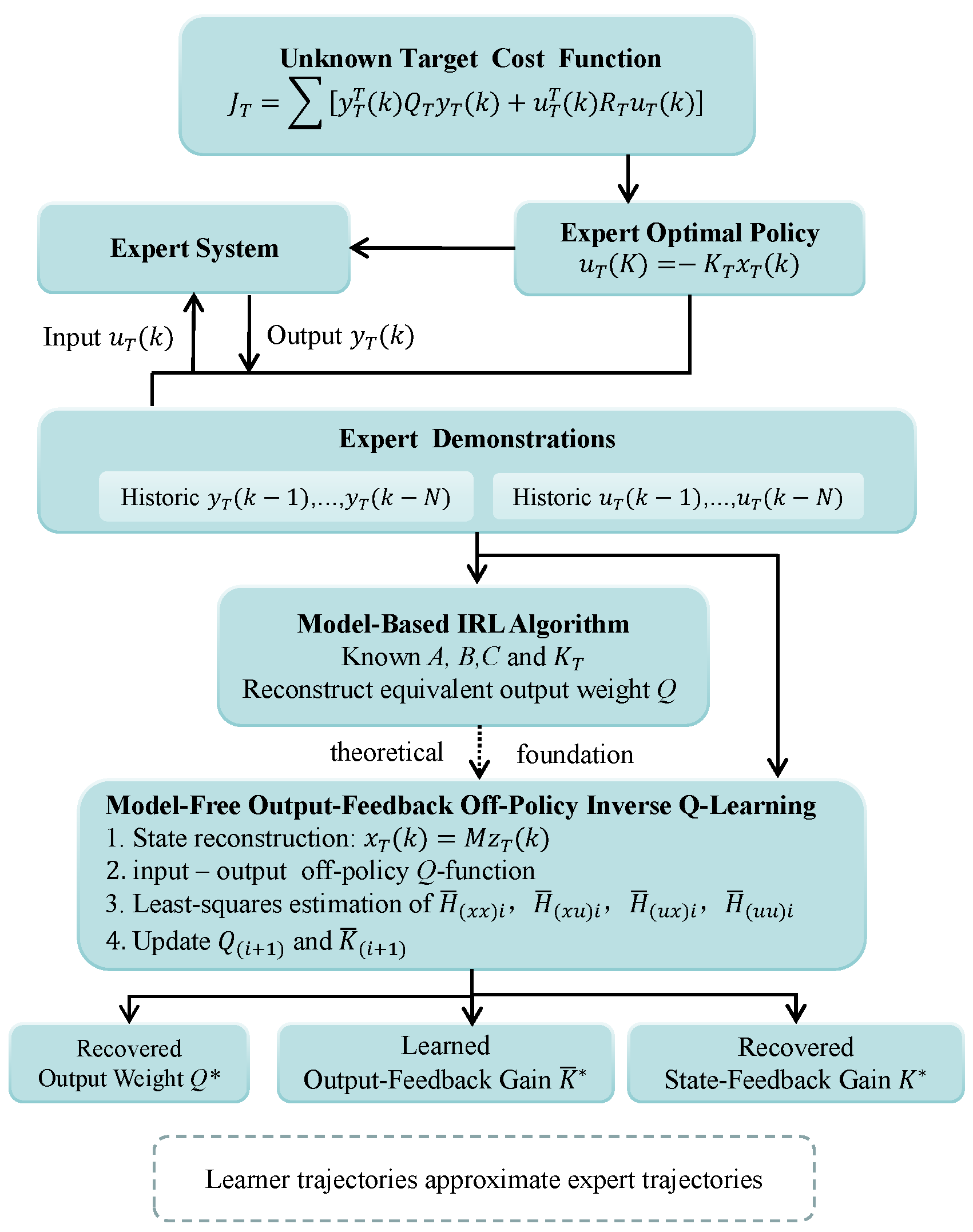
The organization of the paper is as follows. The problem formulation and the inverse reinforcement learning objective are introduced in Section 2. A model-based IRL design, together with its theoretical analysis, is given in Section 3. Section 4 presents the model-free output-feedback off-policy inverse Q-learning approach and discusses both its implementation and analytical results. Simulation examples are provided in Section 5, and the paper is concluded thereafter.

2. Problem Formulation

Consider a linear DT learner system with an unobservable state:

$$\begin{array}{cc}\hfill x(k+1)& =Ax\left(k\right)+Bu\left(k\right),\hfill \\ \hfill y\left(k\right)& =Cx\left(k\right).\hfill \end{array}$$

(1)

where $x\left(k\right)\in {\mathbb{R}}^n$ is the system state, $u\left(k\right)\in {\mathbb{R}}^m$ is the control input, and $y\left(k\right)\in {\mathbb{R}}^q$ is the system output. $A\in {\mathbb{R}}^{n\times n}$ is the state matrix, $B\in {\mathbb{R}}^{n\times m}$ is the input matrix, and $C\in {\mathbb{R}}^{q\times n}$ is the output matrix.

The corresponding expert system is described as

$$\begin{array}{cc}\hfill x_T(k+1)& =A{x}_T\left(k\right)+B{u}_T\left(k\right),\hfill \\ \hfill y_T\left(k\right)& =C{x}_T\left(k\right).\hfill \end{array}$$

(2)

where $x_T\left(k\right)\in {\mathbb{R}}^n$ is the target state, $u_T\left(k\right)\in {\mathbb{R}}^m$ is the target control input, and $y_T\left(k\right)\in {\mathbb{R}}^q$ is the target system output. State matrix A, input matrix B, and output matrix C are the same as the learner system (1).

Remark 1.

The learner system (1) and the expert system (2) share the same system dynamics.

Assumption 1.

The matrix C is full-rank. The pair $(A,B)$ is controllable, and the pair $(A,C)$ is observable.

For expert systems, the following target cost function should be considered:

$$V_T^{*}\left(x_T\left(k\right)\right)=\underset{u_T\left(k\right)}{min}{\displaystyle \sum _{j=k}^{\infty }}\left(y_T^T\left(j\right)Q_T{y}_T\left(j\right)+u_T^T\left(j\right)R_T{u}_T\left(j\right)\right)$$

(3)

where $Q_T^T=Q_T\in {\mathbb{R}}^{q\times q}$ and $R_T^T=R_T\in {\mathbb{R}}^{m\times m}$ are target weight matrices. Equation (3) describes the output-feedback optimal control problem corresponding to the expert system. Since the system state cannot be directly measured, the state will be reconstructed in the subsequent sections using input–output data.

Under the optimal control framework, the target optimal control law of the expert system (2) can be expressed as

$$u_T\left(k\right)=-K_T{x}_T\left(k\right)$$

(4)

where $K_T$ denotes the optimal control gain, which satisfies

$$K_T={(R_T+B^T{P}_{T}B)}^{-1}\left(B^T{P}_{T}A\right)$$

(5)

where $P_T^T=P_T\in {\mathbb{R}}^{n\times n}>0$ satisfies the following target DT algebraic Riccati equation (ARE):

$$P_T=A^T{P}_{T}A+C^T{Q}_{T}C-A^T{P}_{T}B{(R_T+B^T{P}_{T}B)}^{-1}{B}^T{P}_{T}A.$$

(6)

Substituting $K_T$ in (5) into (6) yields

$${(A-B{K}_T)}^T{P}_T(A-B{K}_T)+K_T^T{R}_T{K}_T+C^T{Q}_{T}C-P_T=0.$$

(7)

Equation (7) shows that, under the optimal control strategy, the cost function of the expert system satisfies the corresponding ARE, thereby providing a theoretical foundation for the formulation of subsequent IRL problems.

Assumption 2.

The target weights $Q_T$ and $R_T$ of the expert system (2), as well as the corresponding optimal control gain $K_T$, are unknown to the learner (1).

Assumption 3.

The input–output trajectories $u_T\left(k\right)$ and $y_T\left(k\right)$ of the expert system (2) are available to the learner (1), while the states $x_T\left(k\right)$ of both the expert system and the learner system (1) cannot be observed.

Definition 1

(Equivalent Weight). Given any $R=R^T\in {\mathbb{R}}^{m\times m}>0$, if there exists a $Q\in {\mathbb{R}}^{q\times q}\ge 0$ such that the cost function determined by $(Q,R)$ yields the same $K_T$ as the expert (2), then Q is called an equivalent weight of $Q_T$, and the corresponding cost function is said to be equivalent to the target cost function (3) of the expert system.

Definition 2

(IRL Problem). The objective of IRL is to reconstruct, based only on the input–output trajectory data $(y_T\left(k\right),u_T\left(k\right))$ of the expert system (2), a set of cost-function weight parameters that are equivalent in terms of the target cost function, such that the learner system (1) can not only recover the unknown cost function but also generate the same optimal control policy as that of the expert system (2).

Definition 3.

If there exists a sufficiently small constant $\sigma >0$ such that a matrix or vector X satisfies

$$\parallel X-X^{*}\parallel \le \sigma$$

(8)

then X is called an approximate solution of $X^{*}$.

3. Model-Based IRL Algorithm

To address the aforementioned IRL problem, this section proposes a model-based method. A model-based IRL algorithm is firstly formulated to reconstruct the output weight matrix that equates to the target cost function (3). Furthermore, the algorithm is analysed to serve as the theoretical foundation for subsequent model-free algorithm.

3.1. Optimal Control with Output Feedback and Cost Weighting

For the learner system (1), consider the following infinite-time cost function

$$V\left(x\left(k\right)\right)={\displaystyle \sum _{j=k}^{\infty }}\left(y{\left(j\right)}^{T}Qy\left(j\right)+u{\left(j\right)}^{T}Ru\left(j\right)\right)$$

(9)

where $Q=Q^T\in {\mathbb{R}}^{q\times q}>0$ denotes the output weight matrix, and $R=R^T\in {\mathbb{R}}^{m\times m}>0$ denotes the input weight matrix. In contrast to expert system (2), the objective of a learner system (1) is to solve the following cost function within the framework of optimal control.

$$V^{*}\left(x\left(k\right)\right)=\underset{u\left(k\right)}{min}{\displaystyle \sum _{j=k}^{\infty }}\left(y{\left(j\right)}^{T}Qy\left(j\right)+u{\left(j\right)}^{T}Ru\left(j\right)\right).$$

(10)

When the learner system (1) operates under the optimal control policy, its control input can be expressed as

$$u\left(k\right)=-Kx\left(k\right).$$

(11)

In particular, the control gain K satisfies

$$K={(R+B^{T}PB)}^{-1}{B}^{T}PA$$

(12)

where $P=P^T\in {\mathbb{R}}^{n\times n}>0$ satisfies the following DT ARE:

$$P=A^{T}PA+C^{T}QC-A^{T}PB{(R+B^{T}PB)}^{-1}{B}^{T}PA.$$

(13)

Furthermore, substituting (12) into (13) yields

$${(A-BK)}^{T}P(A-BK)+K^{T}RK+C^{T}QC-P=0.$$

(14)

3.2. Design of Model-Based IRL Algorithms

The objective is to construct a model-based IRL algorithm, given $(A,B,C)$ and $K_T$, for reconstructing the output weight matrix that minimizes the target cost function (3) of an expert system (2). Before we proceed with the algorithm design, the following lemma is stated.

Lemma 1.

Let $R>0$ for the learner system (1). If matrices Q and P both satisfy (14) and

$$\begin{array}{cc}\hfill & {(A-BK)}^{T}P(A-BK)+K^{T}RK+C^{T}QC-P-{(K-K_T)}^{T}R(K-K_T)=0,\hfill \end{array}$$

(15)

then the control gain K obtained is equal to the target control gain $K_T$.

Proof. 

Since Q and P satisfy both (14) and (15), subtracting (14) from (15) yields

$${(K-K_T)}^{T}R(K-K_T)=0,$$

(16)

then

$$K=K_T.$$

(17)

The proof is completed.    □

Based on Lemma 1, a model-based IRL algorithm is proposed. Given an arbitrary symmetric positive definite matrix R, a learning rate $\alpha \in (0,1]$, an initial output weight matrix $Q_0$, and an initial control gain $K_0$, let the iteration number be $i=0,1,2,\dots$. Before designing the algorithm, we present the steps as follows.

(1) 

Policy evaluation $P_i$.

As the algorithm iterates, Equation (14) is rewritten as

$${(A-B{K}_i)}^T{P}_i(A-B{K}_i)+K_i^{T}R{K}_i+C^T{Q}_{i}C-P_i=0.$$

(18)

(2) 

Output weight adjustment $Q_{i+1}$.

Once $P_i$ has been obtained, a correction term corresponding to inverse optimal control [28] is introduced, and the output weight matrix $Q_{i+1}$ is updated using Equation (14). Let

$$\begin{array}{cc}\hfill Q_i& =C^T{Q}_{i}C=P_i-{(A-B{K}_i)}^T{P}_i(A-B{K}_i)-K_i^{T}R{K}_i+{(K_i-K_T)}^{T}R(K_i-K_T).\hfill \end{array}$$

(19)

Correcting the coupling term between the current $Q_i$ in (19) and the $Q_i$ in (15) to $Q_{i+1}$ gives

$$C^T{Q}_{i+1}C=(1-\alpha )C^T{Q}_{i}C+\alpha Q_i.$$

(20)

The pair $(A,B)$ is controllable; the pair $(A,C)$ is observable; and matrix C has full row rank. Substitute (15) and (19) into (20), then multiply ${\left(C{C}^T\right)}^{-1}CC$ and $C^T{\left(C{C}^T\right)}^{-1}$ by the left-hand and right-hand sides, respectively, to obtain

$$\begin{array}{cc}\hfill Q_{i+1}& =Q_i-\alpha {\left(C{C}^T\right)}^{-1}C(C^T{Q}_{i}C-{\overline{Q}}_i)C^T{\left(C{C}^T\right)}^{-1}\hfill \\ \hfill & =Q_i+\alpha {\left(C{C}^T\right)}^{-1}C{(K_i-K_T)}^{T}R(K_i-K_T)C^T{\left(C{C}^T\right)}^{-1}.\hfill \end{array}$$

(21)

(3) 

Control policy update $K_{i+1}$.

Evaluate $P_i$ using the current policy, and update the control policy $K_{i+1}$

$$K_{i+1}={(R+B^T{P}_{i}B)}^{-1}{B}^T{P}_{i}A.$$

(22)

Then set $i=i+1$ and repeat (18)–(22) until the convergence condition $\parallel K_{i+1}-K_i\parallel \le \sigma$ is satisfied, where $\sigma >0$ is a predefined sufficiently small tolerance. The procedure of the model-based IRL algorithm is given in Algorithm 1.

Algorithm 1 Model-Based IRL Algorithm

1: Initialization. Given $R>0$ and $\alpha \in (0,1]$, initialize the algorithm with a reward weighting matrix $Q_0\ge 0$ and a stabilizing gain $K_0$, and set $i=0$. 2: Evaluate $P_i$ as (18). 3: Correct $Q_{i+1}$ by (21). 4: Update $K_{i+1}$ by (22). 5: Update $i=i+1$, and repeat Step 1 until the stopping criterion $\parallel K_{i+1}-K_i\parallel \le \sigma$ is satisfied, where $\sigma >0$ is a prescribed tolerance.

3.3. Theoretical Analysis of Algorithm 1

This subsection presents theoretical results concerning the convergence and stability of the proposed algorithm.

Theorem 1

(Convergence of Algorithm 1). Given $Q_0\ge 0$, $R>0$, and $\alpha \in (0,1]$, if the system $(A,C)$ is observable, the sequence $\left\{Q_i\right\}$ will converge to some equivalent weight Q (see Definition 2), and Algorithm 1 will terminate within a finite number of steps under the given threshold condition.

Proof. 

Following the convergence analysis reported in [4,26,29], one can conclude that Algorithm 1 requires only a finite number of iterations for the update of $Q_i$ to stop.

Multiply the left-hand side and right-hand side of (21) by $C^T$ and C, respectively, to obtain

$$\begin{array}{cc}\hfill C^T{Q}_{i+1}C& =(1-\alpha )C^T{Q}_{i}C+\alpha \left(C^T{Q}_{i}C+{(K_i-K_T)}^{T}R(K_i-K_T)\right)\hfill \\ \hfill & =C^T{Q}_{i}C+\alpha C^T{\left(C{C}^T\right)}^{-1}C{(K_i-K_T)}^{T}R(K_i-K_T)C^T{\left(C{C}^T\right)}^{-1}C.\hfill \end{array}$$

(23)

Let

$${\mathrm{\Sigma }}_i=C^T{\left(C{C}^T\right)}^{-1}C{(K_i-K_T)}^{T}R(K_i-K_T)C^T{\left(C{C}^T\right)}^{-1}C.$$

(24)

Equation (23) can be written as

$$C^T(Q_{i+1}-Q_i)C=\alpha {\mathrm{\Sigma }}_i.$$

(25)

Because ${\mathrm{\Sigma }}_i\ge 0$, there is

$$Q_{i+1}\ge Q_i\ge \dots \ge Q_1\ge 0,i=0,1,\dots$$

(26)

That is, $\left\{Q_i\right\}$ is monotonically increasing. This follows from (25):

$$C^T{Q}_{i+1}C=\alpha {\mathrm{\Sigma }}_i+\alpha {\mathrm{\Sigma }}_{i-1}+\dots +\alpha {\mathrm{\Sigma }}_0+C^T{Q}_0.C$$

(27)

From the Riccati equation theory [30], $P_i$ varies monotonically with $Q_i$, and the associated gain $K_i$ is consequently adjusted. It is also known that the target gain $K_T$ may correspond to infinitely many equivalent weighting matrices Q. Hence, we aim to identify a particular equivalent matrix $Q_e$ such that

$$\parallel Q_i-Q_e\parallel \le \eta$$

(28)

and

$$\parallel K_i-K_T\parallel \le \sigma$$

(29)

and the algorithm stops.

It follows from (26) that

$$\begin{array}{cc}\hfill C^{T}QC& \ge \parallel C^T{Q}_{i+1}C\parallel -{\eta }_0(\eta ,C)=\parallel \alpha {\mathrm{\Sigma }}_i+\dots +\alpha {\mathrm{\Sigma }}_0+C^T{Q}_{0}C\parallel -{\eta }_0,\hfill \end{array}$$

(30)

and it can be further shown that

$$C^{T}QC\ge \alpha (i+1){\sigma }^2{\lambda }_{min}(R+B^{T}PB)-{\eta }_0,$$

(31)

Therefore,

$$i\le {\displaystyle \frac{\parallel C^{T}QC\parallel +{\eta }_0(\eta ,C)}{\alpha {\sigma }^2{\lambda }_{min}R}}-1.$$

(32)

According to Definition 1, $Q_i$ is monotonically increasing and $\parallel Q_i\parallel$ is bounded. Therefore, Algorithm 1 converges within a finite number of steps, and the obtained control gain approaches $K_T$. The proof is completed.    □

Remark 2.

As discussed after Theorem 1, the equivalent output weight matrix is generally non-unique. Different choices of R and $Q_0$ may yield different converged matrices $Q_{\infty }$, while the resulting pair $(Q_{\infty },R)$ generates the same optimal policy $K_T$. In practice, $R=I$ and $Q_0=\lambda I$ with a small $\lambda >0$ provide a simple default choice for stable and monotonic convergence. In particular, $Q_0=0$ and $R=I$ can be used as a convenient minimum-norm selection criterion.

Theorem 2

(Stability of the closed-loop system). At every iteration step of Algorithm 1, the closed-loop system of the learner system (1) is stable.

Proof. 

Given an initial $Q_0$ and $R>0$, the closed-loop stability of the system must be ensured [31] to prove that

$$V_i\left(x(k+1)\right)-V_i\left(x\left(k\right)\right)\le 0.$$

(33)

If we define the Lyapunov function corresponding to the ith iteration as

$$V_i\left(x\left(k\right)\right)=x^T\left(k\right)P_{i}x\left(k\right),$$

(34)

then there is

$$\begin{array}{c}{V}_i\left(x(k+1)\right)-V_i\left(x\left(k\right)\right)=x^T\left(k\right)\left[{(A-B{K}_i)}^T{P}_i(A-B{K}_i)-P_i\right]x\left(k\right),\end{array}$$

(35)

where $P_i>0$; combining Equations (18) and (35) yields

$$\begin{array}{c}{V}_i\left(x(k+1)\right)-V_i\left(x\left(k\right)\right)=-x^T\left(k\right)\left(K_i^{T}R{K}_i+C^T{Q}_{i}C\right)x\left(k\right).\end{array}$$

(36)

Since $R>0$ and $Q_i\ge 0$, it follows that

$$K_i^{T}R{K}_i+C^T{Q}_{i}C\ge 0,$$

(37)

and thus,

$$V_i\left(x(k+1)\right)-V_i\left(x\left(k\right)\right)\le 0.$$

(38)

Consequently, the stability of the learner system (1) is guaranteed throughout the entire iterative process. This completes the proof.    □

4. Model-Free Output-Feedback Off-Policy Inverse Q-Learning Algorithm

In practical control systems, uncertainty in the system model limits the effectiveness of model-based methods. Moreover, unobservable states make it difficult to implement traditional control strategies that rely on full-state information. To address these issues, building upon Algorithm 1, we propose a data-driven, output-feedback method that reconstructs the unknown target cost function using only input–output data from the expert system (2).

4.1. Establishment of Off-Policy Q-Function Equation

For the ith iteration, multiply the left side of (18) by $x_T^T\left(k\right)$ and the right side by $x_T\left(k\right)$, resulting in

$$\begin{array}{cc}\hfill & x_T^T\left(k\right){(A-B{K}_i)}^T{P}_i(A-B{K}_i)x_T\left(k\right)+x_T^T\left(k\right)K_i^{T}R{K}_i{x}_T\left(k\right)\hfill \\ \hfill & +x_T^T\left(k\right)C^T{Q}_{i}C{x}_T\left(k\right)-x_T^T\left(k\right)P_i{x}_T\left(k\right)=0.\hfill \end{array}$$

(39)

Define the expert’s state Q-function as

$$\begin{array}{cc}\hfill & Q_i(x_T\left(k\right),P_i)\hfill \\ \hfill & =x_T^T\left(k\right)P_i{x}_T\left(k\right)\hfill \\ \hfill & ={(A{x}_T\left(k\right)+B{K}_i{x}_T\left(k\right))}^T{P}_i(A{x}_T\left(k\right)+B{K}_i{x}_T\left(k\right))+x_T^T\left(k\right)C^T{Q}_{i}C{x}_T\left(k\right)+x_T^T\left(k\right)K_i^{T}R{K}_i{x}_T\left(k\right)\hfill \\ \hfill & ={\left[\begin{array}{c}{x}_T\left(k\right)\\ K_i{x}_T\left(k\right)\end{array}\right]}^T{H}_i\left[\begin{array}{c}{x}_T\left(k\right)\\ K_i{x}_T\left(k\right)\end{array}\right]\hfill \\ \hfill & =x_T^T\left(k\right)W_i^T{H}_i{W}_i{x}_T\left(k\right).\hfill \end{array}$$

(40)

where

$$W_i=\left[\begin{array}{c}I\\ -K_i\end{array}\right]$$

(41)

and

$$\begin{array}{cc}\hfill H_i& =\left[\begin{array}{cc}{H}_{\left(xx\right)i}& H_{\left(xu\right)i}\\ H_{\left(ux\right)i}& H_{\left(uu\right)i}\end{array}\right]\hfill \\ \hfill & =\left[\begin{array}{cc}{A}^T{P}_{i}A+C^T{Q}_{i}C& A^T{P}_{i}B\\ B^T{P}_{i}A& R+B^T{P}_{i}B\end{array}\right];\hfill \end{array}$$

(42)

the block matrix is defined as

$$\begin{array}{cc}\hfill H_{\left(xx\right)i}& =A^T{P}_{i}A+C^T{Q}_{i}C\in {\mathbb{R}}^{n\times n},\hfill \\ \hfill H_{\left(xu\right)i}& =A^T{P}_{i}B\in {\mathbb{R}}^{n\times m},\hfill \\ \hfill H_{\left(ux\right)i}& =B^T{P}_{i}A\in {\mathbb{R}}^{m\times n},\hfill \\ \hfill H_{\left(uu\right)i}& =B^T{P}_{i}B+R\in {\mathbb{R}}^{m\times m}.\hfill \end{array}$$

(43)

Next, we construct the off-policy equation using the off-policy method [32]. The original expert system (2) is rewritten as

$$x_T(k+1)=A_c{x}_T\left(k\right)+B\left(u_T\left(k\right)+K_i{x}_T\left(k\right)\right)$$

(44)

where $A_c=A-B{K}_i$, $u_i=-K_i{x}_T\left(k\right)$ denotes the auxiliary control input for system (2), while $u_T\left(k\right)$ denotes the target control input.

Multiplying the left-hand side and right-hand side of (14) by $x_T^T\left(k\right)$ and $x_T\left(k\right)$, respectively, and substituting (40) and (44) into it, one obtains

$$\begin{array}{cc}\hfill & x_T^T\left(k\right)W_i^T{H}_i{W}_i{x}_T\left(k\right){(x_T(k+1)-B(u_T\left(k\right)+K_i{x}_T\left(k\right)))}^T{P}_i(x_T(k+1)-B(u_T\left(k\right)+K_i{x}_T\left(k\right)))\hfill \\ \hfill & =x_T^T\left(k\right)C^T{Q}_{i}C{x}_T\left(k\right)+x_T^T\left(k\right)K_i^{T}R{K}_i{x}_T\left(k\right).\hfill \end{array}$$

(45)

Substituting $P_i=W_i^T{H}_i{W}_i$ from (40) into (45) and expanding the quadratic form on the left-hand side, one obtains

$$\begin{array}{cc}\hfill & x_T^T\left(k\right)W_i^T{H}_i{W}_i{x}_T\left(k\right)-x_T^T(k+1)W_i^T{H}_i{W}_i{x}_T(k+1)\hfill \\ \hfill & +2x_T^T(k+1)P_{i}B\left(u_T\left(k\right)+K_i{x}_T\left(k\right)\right)\hfill \\ \hfill & -{\left(u_T\left(k\right)+K_i{x}_T\left(k\right)\right)}^T{B}^T{P}_{i}B\left(u_T\left(k\right)+K_i{x}_T\left(k\right)\right)\hfill \\ \hfill & =x_T^T\left(k\right)C^T{Q}_{i}C{x}_T\left(k\right)+x_T^T\left(k\right)K_i^{T}R{K}_i{x}_T\left(k\right).\hfill \end{array}$$

(46)

It follows from (40) and (42) that

$$\begin{array}{cc}\hfill & Q_i(x_T\left(k\right),P_i)\hfill \\ \hfill & =x_T^T\left(k\right)H_{\left(xx\right)i}{x}_T\left(k\right)+2x_T^T\left(k\right)H_{\left(xu\right)i}{u}_T\left(k\right)+u_T^T\left(k\right)H_{\left(uu\right)i}{u}_T\left(k\right).\hfill \end{array}$$

(47)

It follows from Q-functions (40) and (47) that

$$\begin{array}{cc}\hfill & x_T^T\left(k\right)H_{\left(xx\right)i}{x}_T\left(k\right)+2x_T^T\left(k\right)H_{\left(xu\right)i}{u}_T\left(k\right)+u_T^T\left(k\right)H_{\left(uu\right)i}{u}_T\left(k\right)\hfill \\ \hfill & =x_T^T\left(k\right)C^T{Q}_{i}C{x}_T\left(k\right)+u_T^T\left(k\right)R{u}_T\left(k\right)+x_T^T(k+1)P_i{x}_T(k+1).\hfill \end{array}$$

(48)

Combining this with (41) and (48) yields

$$\begin{array}{cc}\hfill & x_T^T\left(k\right)H_{\left(xx\right)i}{x}_T\left(k\right)-x_T^T(k+1)H_{\left(xx\right)i}{x}_T(k+1)\hfill \\ \hfill & +2x_T^T\left(k\right)H_{\left(xu\right)i}{u}_T\left(k\right)+2x_T^T(k+1)H_{\left(xu\right)i}{K}_i{x}_T(k+1)\hfill \\ \hfill & -u_T^T\left(k\right)H_{\left(uu\right)i}{u}_T\left(k\right)-x_T^T(k+1)K_i^T{H}_{\left(uu\right)i}{K}_i{x}_T(k+1)\hfill \\ \hfill & =x_T^T\left(k\right)C^T{Q}_{i}C{x}_T\left(k\right)+u_T^T\left(k\right)R{u}_T\left(k\right).\hfill \end{array}$$

(49)

Thus the off-policy Q-function equation is obtained. Using the least-squares method and the expert state-input data $x_T\left(k\right)$ and $u_T\left(k\right)$, Equation (49) yields a unique solution ($H_{\left(xx\right)i}$, $H_{\left(xu\right)i}$, $H_{\left(ux\right)i}$$H_{\left(uu\right)i}$) without knowledge of the system dynamics.

4.2. Design of a Output-Feedback Off-Policy Inverse Q-Learning Algorithm

We now proceed to design a model-free method based on the aforementioned off-policy Q-function Equation (49). First, using a state reconstruction method, the off-policy Q-function Equation (49) is transformed into an input–output off-policy Q-function equation. We then iteratively update the output-reward weights $Q_i$ and control gains $K_i$ based on this input–output Q-function.

As shown in Assumption 3, $x_T\left(k\right)$ is unobservable, whereas $u_T\left(k\right)$ and $y_T\left(k\right)$ are available. By introducing the lemma from Reference [33], the input and output data $u_T\left(k\right)$ and $y_T\left(k\right)$ are used to represent the Q-function without using the state $x_T\left(k\right)$.

Lemma 2.

If Assumption 1 holds, the system state $x_T\left(k\right)$ at time k can be expressed in terms of the measurable input and output sequences from $(k-N)$ to $(k-1)$, as shown below:

$$x_T\left(k\right)=M_y{\overline{y}}_{k-1,k-N}+M_u{\overline{u}}_{k-1,k-N}$$

(50)

where $N\le n$ is the upper bound of the observability index of the system, while ${\overline{u}}_{k-1,k-N}\in {\mathbb{R}}^{m\times N}$ and ${\overline{y}}_{k-1,k-N}\in {\mathbb{R}}^{s\times N}$, respectively, denote the stacked input and output data vectors,

$$\begin{array}{cc}\hfill {\overline{u}}_{k-1,k-N}& ={\left[u_T^T(k-1)u_T^T(k-2)\dots u_T^T(k-N)\right]}^T,\hfill \\ \hfill {\overline{y}}_{k-1,k-N}& ={\left[y_T^T(k-1)y_T^T(k-2)\dots y_T^T(k-N)\right]}^T.\hfill \end{array}$$

(51)

The coupling matrix is defined as

$$\begin{array}{cc}\hfill M_u& =U_N-A^N{\left(V_N^T{V}_N\right)}^{-1}{V}_N^T{G}_N,\hfill \\ \hfill M_y& =A^N{\left(V_N^T{V}_N\right)}^{-1}{V}_N^T\hfill \end{array}$$

(52)

and

$$V_N={\left[{\left(C{A}^{N-1}\right)}^T\dots {\left(CA\right)}^T{C}^T\right]}^T$$

(53)

$$U_N=\left[BAB\dots A^{N-1}B\right]$$

(54)

$$G_N=\left[\begin{array}{ccccc}0& CB& CAB& \dots & C{A}^{N-2}B\\ 0& 0& CB& \dots & C{A}^{N-3}B\\ ⋮& ⋮& ⋮& \ddots & ⋮\\ 0& \dots & \dots & 0& CB\\ 0& 0& 0& \dots & 0.\end{array}\right]$$

(55)

where $V_N$ is the observable matrix, $U_N$ is the control matrix representing the control inputs, and $G_N$ is the Toeplitz matrix. Therefore, the state $x_T\left(k\right)$ can be expressed in terms of the input–output data as

$$x_T\left(k\right)=M{z}_T\left(k\right)$$

(56)

where

$$\begin{array}{cc}\hfill z_T\left(k\right)& ={\left[{\overline{u}}_{k-1,k-N}{\overline{y}}_{k-1,k-N}\right]}^T,\hfill \\ \hfill M& =\left[M_u{M}_y\right].\hfill \end{array}$$

(57)

By using the input–output data description (56) of the operating state to describe the state feedback Q-function (40), it is possible to obtain the input–output Q-function as follows:

$$Q_i(z_T\left(k\right),P_i)=z_T{\left(k\right)}^T{M}^T{W}_i^T{H}_i{W}_{i}M{z}_T\left(k\right).$$

(58)

The input–output Q-function matrix is further defined as

$${\overline{H}}_i=\left[\begin{array}{cc}{\overline{H}}_{\left(xx\right)i}& {\overline{H}}_{\left(xu\right)i}\\ {\overline{H}}_{\left(ux\right)i}& {\overline{H}}_{\left(uu\right)i}\end{array}\right]$$

(59)

where ${\overline{H}}_i={\overline{H}}_i^T\in {\mathbb{R}}^{f\times f}$, $f=mN+qN+m$, and the block matrix is defined as follows:

$$\begin{array}{cc}\hfill {\overline{H}}_{\left(xx\right)i}& =M^T(A^T{P}_{i}A+C^T{Q}_{i}C)M\in {\mathbb{R}}^{(m+q)N\times (m+q)N},\hfill \\ \hfill {\overline{H}}_{\left(xu\right)i}& =M^T{A}^T{P}_{i}B\in {\mathbb{R}}^{(m+q)N\times m},\hfill \\ \hfill {\overline{H}}_{\left(ux\right)i}& =B^T{P}_{i}AM\in {\mathbb{R}}^{m\times (m+q)N},\hfill \\ \hfill {\overline{H}}_{\left(uu\right)i}& =B^T{P}_{i}B+R\in {\mathbb{R}}^{m\times m}.\hfill \end{array}$$

(60)

Taking into account (22) and (59), the optimal control gain ${\overline{K}}_i^T$ of the input–output Q function can be expressed as

$${\overline{K}}_{i+1}=K_{i+1}M.$$

(61)

Here, $K_{i+1}$ denotes the state feedback gain, while ${\overline{K}}_{i+1}$ denotes the equivalent output-feedback gain acting on $z_T\left(k\right)$; it follows from the block structure of the state-dependent Q-function matrix $H_i$ that

$$K_{i+1}=H_{\left(uu\right)i}^{-1}{H}_{\left(ux\right)i}.$$

(62)

Therefore, there is

$${\overline{K}}_{i+1}=K_{i+1}M=H_{\left(uu\right)i}^{-1}{H}_{\left(ux\right)i}M={\overline{H}}_{\left(uu\right)i}^{-1}{\overline{H}}_{\left(ux\right)i}.$$

(63)

By introducing probing noise into the auxiliary control input, ${\widehat{u}}_T\left(k\right)=u_T\left(k\right)+ϵ\left(k\right)$, and substituting it into (49), the output-feedback off-policy Q-function equation can be obtained as

$$\begin{array}{cc}\hfill & z_T^T\left(k\right){\overline{H}}_{\left(xx\right)i}{z}_T\left(k\right)-z_T^T(k+1){\overline{H}}_{\left(xx\right)i}{z}_T(k+1)\hfill \\ \hfill & +2z_T^T\left(k\right){\overline{H}}_{\left(xu\right)i}{\widehat{u}}_T\left(k\right)+2z_T^T(k+1){\overline{H}}_{\left(xu\right)i}{\overline{K}}_i{z}_T(k+1)\hfill \\ \hfill & +{\widehat{u}}_T^T\left(k\right){\overline{H}}_{\left(uu\right)i}{\widehat{u}}_T\left(k\right)-z_T^T(k+1){\overline{K}}_i^T{\overline{H}}_{\left(uu\right)i}{\overline{K}}_i{z}_T(k+1)\hfill \\ \hfill & =y_T^T\left(k\right)Q_i{y}_T\left(k\right)+{\widehat{u}}_T^T\left(k\right)R{\widehat{u}}_T\left(k\right)\hfill \end{array}$$

(64)

where $ϵ\left(k\right)$ represents the probing noise, while $\overline{K_i}$ denotes the output-feedback control gain corresponding to the input–output Q-function. Without prior information on the system dynamics, the components $({\overline{H}}_{\left(xx\right)i}$, ${\overline{H}}_{\left(xu\right)i}$, ${\overline{H}}_{\left(ux\right)i}$${\overline{H}}_{\left(uu\right)i})$ are estimated using the least-squares method by solving Equation (64).

Next, as in Algorithm 1 for correcting $Q_{i+1}$, multiply both sides of (21) by $M{z}_T\left(k\right)$ and substitute $y_T\left(k\right)=C{x}_T\left(k\right)$:

$$\begin{array}{cc}\hfill & y_T^T\left(k\right)Q_{i+1}{y}_T\left(k\right)\hfill \\ \hfill & =y_T^T\left(k\right)Q_i{y}_T\left(k\right)+\alpha {\left({\widehat{u}}_T\left(k\right)+{\overline{K}}_i{z}_T\left(k\right)-ϵ\left(k\right)\right)}^{T}R({\widehat{u}}_T\left(k\right)+{\overline{K}}_i{z}_T\left(k\right)-ϵ\left(k\right)),\hfill \end{array}$$

(65)

where ${\overline{K}}_{i+1}$ is updated iteratively according to (63). Finally, repeat the above steps until the convergence condition $\parallel K_{i+1}-K_i\parallel <\sigma$ is satisfied; otherwise, set $i=i+1$ and proceed to (64). The above computational procedure is summarized in Algorithm 2.

Algorithm 2 Model-Free Output-Feedback Off-Policy Inverse Q-Learning Algorithm

1: Initialization: Given $R>0$, initialize the algorithm with a reward weighting matrix $Q_0\ge 0$ and a stabilizing gain $K_0$, and set $i=0$. 2: Evaluate ${\overline{H}}_{\left(xx\right)i},{\overline{H}}_{\left(xu\right)i},{\overline{H}}_{\left(ux\right)i},{\overline{H}}_{\left(uu\right)i}$ by (65). 3: Improve $Q_{i+1}$ as (65). 4: Update ${\overline{K}}_{i+1}$ by (63). 5: Update $i=i+1$, and repeat Step 1 until the stopping criterion $\parallel {\overline{K}}_{i+1}-{\overline{K}}_i\parallel \le \sigma$ is satisfied, where $\sigma >0$ is a prescribed tolerance.

Remark 3.

Lemma 2 reveals that the system state $x_T\left(k\right)$ can be reconstructed from past input–output data. The parameter N is the observability index, which represents the minimum number of past output samples needed to uniquely determine the current state.

4.3. Implementation of the Model-Free Algorithm

This subsection shows the implementation of steps (64) and (65) of Algorithm 2. The implementation of this algorithm primarily utilizes the following Kronecker product:

$$a^{T}Wb=(b^T\otimes a^T)\mathrm{vec}\left(W\right).$$

(66)

Using the Kronecker product in (66), estimate ${\overline{H}}_{\left(xx\right)i},{\overline{H}}_{\left(xu\right)i},{\overline{H}}_{\left(ux\right)i},{\overline{H}}_{\left(uu\right)i}$ via (64), where (64) is rewritten as

$$\begin{array}{cc}\hfill & \left(z_T^T\left(k\right)\otimes z_T^T\left(k\right)-z_T^T(k+1)\otimes z_T^T(k+1)\right)\mathrm{vec}\left({\overline{H}}_{\left(xx\right)i}\right)\hfill \\ \hfill & +2\left({\widehat{u}}_T^T\left(k\right)\otimes z_T^T\left(k\right)+{\overline{K}}_i{z}_T(k+1)\otimes z_T^T(k+1)\right)\mathrm{vec}\left({\overline{H}}_{\left(xu\right)i}\right)\hfill \\ \hfill & +\left({\widehat{u}}_T^T\left(k\right)\otimes {\widehat{u}}_T^T\left(k\right)-{\left({\overline{K}}_i{z}_T(k+1)\right)}^T\otimes {\left({\overline{K}}_i{z}_T(k+1)\right)}^T\right)\mathrm{vec}\left({\overline{H}}_{\left(uu\right)i}\right)\hfill \\ \hfill & =y_T^T\left(k\right)Q_i{y}_T\left(k\right)+{\widehat{u}}_T^T\left(k\right)R{\widehat{u}}_T\left(k\right).\hfill \end{array}$$

(67)

Using a set of sample data indexed by $l\in {\mathbb{Z}}^{+}$,

$${\varphi }_i={\left[\begin{array}{c}{\varphi }_i^1{\varphi }_i^2\dots {\varphi }_i^l\end{array}\right]}^T$$

(68)

$${\psi }_i=\left[\begin{array}{ccc}{Z}_{\left(xx\right)1}& Z_{\left(xu\right)1}& Z_{\left(uu\right)1}\\ Z_{\left(xx\right)2}& Z_{\left(xu\right)2}& Z_{\left(uu\right)2}\\ ⋮& ⋮& ⋮\\ Z_{\left(xx\right)l}& Z_{\left(xu\right)l}& Z_{\left(uu\right)l}\end{array}\right].$$

(69)

The scalar term corresponding to the lth sample is defined as

$$\begin{array}{cc}\hfill {\varphi }_i^l& =y_T^T(k+l-1)Q_i{y}_T(k+l-1)+{\widehat{u}}_T^T(k+l-1)R{\widehat{u}}_T(k+l-1),\hfill \end{array}$$

(70)

$$\begin{array}{cc}\hfill Z_{\left(xx\right)l}& =z_T^T(k+l-1)\otimes z_T^T(k+l-1)-z_T^T(k+l)\otimes z_T^T(k+l),\hfill \\ \hfill Z_{\left(xu\right)l}& =2\left({\widehat{u}}_T^T(k+l-1)\otimes z_T^T(k+l-1)+{\left({\overline{K}}_i{z}_T(k+l)\right)}^T\otimes z_T^T(k+l)\right),\hfill \\ \hfill Z_{\left(uu\right)l}& ={\widehat{u}}_T^T(k+l-1)\otimes {\widehat{u}}_T^T(k+l-1)-{\left({\overline{K}}_i{z}_T(k+l)\right)}^T\otimes {\left({\overline{K}}_i{z}_T(k+l)\right)}^T.\hfill \end{array}$$

(71)

Then, considering (68)–(71), (67) can be rewritten as

$${\psi }_i{\left[\mathrm{vec}\left({\overline{H}}_{\left(xx\right)i}\right)\mathrm{vec}\left({\overline{H}}_{\left(xu\right)i}\right)\mathrm{vec}\left({\overline{H}}_{\left(uu\right)i}\right)\right]}^T={\varphi }_i.$$

(72)

For (72), using the batch least-squares (BLS) method, one can determine from (68) that

$$\begin{array}{cc}\hfill & {\left[\mathrm{vec}\left({\overline{H}}_{\left(xx\right)i}\right)\mathrm{vec}\left({\overline{H}}_{\left(xu\right)i}\right)\mathrm{vec}\left({\overline{H}}_{\left(uu\right)i}\right)\right]}^T={\left({\psi }_i^T{\psi }_i\right)}^{-1}{\psi }_i^T{\varphi }_i\hfill \end{array}$$

(73)

where the total number of unknown parameters corresponding to $\mathrm{vec}\left({\overline{H}}_{\left(xx\right)i}\right)$, $\mathrm{vec}\left({\overline{H}}_{\left(xu\right)i}\right)$, and $\mathrm{vec}\left({\overline{H}}_{\left(uu\right)i}\right)$ is required to satisfy $l\ge {\left((m+s)N\right)}^2+(m+s)Nm+m^2$. Therefore, in order to guarantee a unique solution to (73), the persistence of excitation condition must be satisfied, and at least $l\ge {\left((m+s)N\right)}^2+(m+s)Nm+m^2$ sampling steps are required. Similar to (66), (65) can be rewritten as

$$\begin{array}{cc}\hfill & {(y_T^T\left(k\right)\otimes y_T^T\left(k\right))}^T\mathrm{vec}\left(Q_{i+1}\right)\hfill \\ \hfill & =y_T^T\left(k\right)Q_i{y}_T\left(k\right)+\alpha {\left({\widehat{u}}_T\left(k\right)+{\overline{K}}_i{z}_T\left(k\right)-ϵ\left(k\right)\right)}^{T}R\left({\widehat{u}}_T\left(k\right)+{\overline{K}}_i{z}_T\left(k\right)-ϵ\left(k\right)\right).\hfill \end{array}$$

(74)

To further utilize multiple groups of sampled data to perform batch least-squares estimation of $Q_{i+1}$, the right-hand side of (74) corresponding to the pth sample group is denoted by ${\xi }_p$. By stacking the regression vectors corresponding to p consecutive groups of sampled data, one obtains the batch data matrix, denoted by ${\eta }_p$, and then one has

$$\begin{array}{cc}\hfill {\xi }_p& =\alpha {\left({\widehat{u}}_T(k+p-1)+{\overline{K}}_i{z}_T(k+p-1)-ϵ(k+p-1)\right)}^T\hfill \\ \hfill & \times R\left({\widehat{u}}_T(k+p-1)+{\overline{K}}_i{z}_T(k+p-1)-ϵ(k+p-1)\right)\hfill \\ \hfill & +y_T^T(k+p-1)Q_i{y}_T(k+p-1)\hfill \end{array}$$

(75)

and

$${\eta }_p=\left[\begin{array}{c}{y}_T^T\left(k\right)\otimes y_T^T\left(k\right)\\ y_T^T(k+1)\otimes y_T^T(k+1)\\ ⋮\\ y_T^T(k+p-1)\otimes y_T^T(k+p-1)\end{array}\right].$$

(76)

where $p\in {\mathbb{Z}}^{+}$ denotes the number of sample data groups.

After multiple sets of sample data are stacked, a batch of linear equations relating to the parameters to be estimated can be formulated and solved using the BLS method; rewriting (74) yields

$$\mathrm{vec}\left(Q_{i+1}\right)={\left({\eta }_p^T{\eta }_p\right)}^{-1}{\eta }_p^T{\xi }_p.$$

(77)

In particular, $Q_{i+1}$ is a symmetric positive definite matrix with ${\displaystyle \frac{q(q+1)}{2}}$ distinct elements, and at least $p\ge {\displaystyle \frac{q(q+1)}{2}}$ samples are required to solve (74).

After multiple sets of sample data are stacked, a system of linear equations involving $\mathrm{vec}\left(Q_{i+1}\right)$ can be formulated, and the latest output weight matrix $Q_{i+1}$ can be obtained using a least-squares approach.

Remark 4.

In Algorithm 2, the dimension of the regressor $z_T\left(k\right)$ is $(m+q)N$, and so the number of unknowns in the input–output Q-function matrix ${\overline{H}}_i$ grows quadratically with N. The per-iteration complexity of the batch least-squares solution is $O\left({((m+q)N+m)}^3\right)$, since the matrix to be inverted has dimension $d=\left(\right(m+q)N+m)\left(\right(m+q)N+m+1)/2$. Therefore, choosing N as the observability index balances reconstruction accuracy and computational efficiency.

Remark 5.

It should be noted that, in order to satisfy the persistence of excitation condition for the BLS problem [32], the auxiliary control input is injected with probing noise in Algorithm 2. This ensures sufficient excitation of the regression data, such that the parameter matrices can be uniquely identified. The unbiasedness of the algorithm after the introduction of probing noise will be rigorously analysed in the subsequent subsection.

4.4. Theoretical Analysis of Algorithm 2

In this subsection, some theoretical results are presented for the proposed algorithm, primarily concerning its unbiasedness and convergence.

Theorem 3

(Unbiasedness of Algorithm 2). In Algorithm 2, by injecting probing noise into the control input ${\widehat{u}}_T\left(k\right)$, the solutions of $({\overline{H}}_{\left(xx\right)i},{\overline{H}}_{\left(xu\right)i},{\overline{H}}_{\left(uu\right)i})$ obtained from (64) and $Q_{i+1}$ obtained from (65) are unbiased, ${\widehat{H}}_{\left(xx\right)i}={\overline{H}}_{\left(xx\right)i},{\widehat{H}}_{\left(xu\right)i}={\overline{H}}_{\left(xu\right)i},{\widehat{H}}_{\left(uu\right)i}={\overline{H}}_{\left(uu\right)i},{\widehat{Q}}_i=Q_i.$

Proof. 

When the control input is injected with probing noise, we have

$${\widehat{u}}_T\left(k\right)=u_T\left(k\right)+ϵ\left(k\right).$$

(78)

According to Lemma 2, Equation (49) is equivalent to (64) and is derived from (44). Therefore, we revisit (44) to analyse the unbiasedness of Algorithm 2. Assume that the control input ${\widehat{u}}_T\left(k\right)$ with injected probing noise leads to biased estimates ${\widehat{H}}_i$ and ${\widehat{Q}}_i$ from (64) and (65), respectively. By substituting ${\widehat{u}}_T\left(k\right)=u_T\left(k\right)+ϵ\left(k\right)$ and the biased estimates ${\widehat{H}}_i$ into (44), one obtains

$$\begin{array}{cc}\hfill & x_T^T\left(k\right)W_i^T{\widehat{H}}_i{W}_i{x}_T\left(k\right)-x_T^T(k+1)W_i^T{\widehat{H}}_i{W}_i{x}_T(k+1)\hfill \\ \hfill & +2x_T^T(k+1){\widehat{P}}_{i}B\left({\widehat{u}}_T\left(k\right)+K_i{x}_T\left(k\right)-ϵ\left(k\right)\right)\hfill \\ \hfill & -{\left(B(u_T\left(k\right)+K_i{x}_T\left(k\right)-ϵ\left(k\right))\right)}^T{\widehat{P}}_i\left(B(u_T\left(k\right)+K_i{x}_T\left(k\right)-ϵ\left(k\right))\right)\hfill \\ \hfill & =x_T^T\left(k\right)C^T{Q}_{i}C{x}_T\left(k\right)+x_T^T\left(k\right)K_i^{T}R{K}_i{x}_T\left(k\right).\hfill \end{array}$$

(79)

If one substitutes $P_i=W_i^T{H}_i{W}_i$ into the terms involving $ϵ\left(k\right)$ and cancelling the common terms, it follows that

$$\begin{array}{cc}\hfill & x_T^T\left(k\right)W_i^T{\widehat{H}}_i{W}_i{x}_T\left(k\right)-x_T^T(k+1)W_i^T{\widehat{H}}_i{W}_i{x}_T(k+1)\hfill \\ \hfill & +2x_T^T(k+1){\widehat{P}}_{i}B\left(u_T\left(k\right)+K_i{x}_T\left(k\right)\right)\hfill \\ \hfill & -{\left(B({\widehat{u}}_T\left(k\right)+K_i{x}_T\left(k\right))\right)}^T{\widehat{P}}_i\left(B({\widehat{u}}_T\left(k\right)+K_i{x}_T\left(k\right))\right)\hfill \\ \hfill & =x_T^T\left(k\right)C^T{Q}_{i}C{x}_T\left(k\right)+x_T^T\left(k\right)K_i^{T}R{K}_i{x}_T\left(k\right).\hfill \end{array}$$

(80)

By comparing the state feedback (44) without probing noise and the state feedback (71) with probing noise, it can conclude that ${\widehat{H}}_i$ = $H_i$. Furthermore, by combining this with the one-to-one correspondence between the input–output form and the state feedback form, it follows that

$${\widehat{H}}_{\left(xx\right)i}={\overline{H}}_{\left(xx\right)i},{\widehat{H}}_{\left(xu\right)i}={\overline{H}}_{\left(xu\right)i},{\widehat{H}}_{\left(uu\right)i}={\overline{H}}_{\left(uu\right)i}.$$

This implies that, after probing noise is introduced, (65) does not introduce bias into $Q_i(z_T\left(k\right),P_i)$.

$$\begin{array}{cc}\hfill & y_T^T\left(k\right){\widehat{Q}}_{i+1}{y}_T\left(k\right)\hfill \\ \hfill & =y_T^T\left(k\right){\widehat{Q}}_i{y}_T\left(k\right)+\alpha {\left(u_T\left(k\right)+{\overline{K}}_i{z}_T\left(k\right)\right)}^{T}R\left(u_T\left(k\right)+{\overline{K}}_i{z}_T\left(k\right)\right).\hfill \end{array}$$

(81)

Thus, it follows that ${\widehat{Q}}_{i+1}=Q_{i+1}$. Then, Algorithm 2 is unbiased with respect to the probing noise. This concludes the proof. □

Theorem 4

(Convergence of Algorithm 2). Given an initial matrix $Q_0>0$, and $(A,\sqrt{Q_0}C)$ is observable, the sequences $\left\{Q_i\right\}$, $\left\{K_i\right\}$, and $\left\{H_i\right\}$ generated by Algorithm 2 converge to the limit matrices $Q_{\infty }$, $K_{\infty }$, and $H_{\infty }$, respectively.

Proof. 

The core of this proof is to establish the mathematical equivalence between Algorithm 2 and the model-based Algorithm 1, whose convergence has been proven in Theorem 1. We demonstrate that every computational step in Algorithm 2 is an algebraically identical transformation of the corresponding step in Algorithm 1, performed solely using input–output data.

The proof proceeds by analysing the three main steps of both algorithms.

Step 1: Equivalence of the Policy Evaluation Steps.

In Algorithm 2, the policy evaluation step solves for the input–output Q-function blocks $({\overline{H}}_{\left(xx\right)i},{\overline{H}}_{\left(xu\right)i},{\overline{H}}_{\left(uu\right)i})$ using (64). By Lemma 2, $x_T\left(k\right)=M{z}_T\left(k\right)$, and from (59) and (60), ${\overline{H}}_i=M^T{H}_{i}M$. Substituting these into (64) transforms it back into the state-feedback off-policy Equation (49). Reversing the off-policy transformation from (44) to (49) yields the state Q-function form:

$$Q_i(x_T\left(k\right),P_i)={\left[\begin{array}{c}{x}_T\left(k\right)\\ -K_i{x}_T\left(k\right)\end{array}\right]}^T{H}_i\left[\begin{array}{c}{x}_T\left(k\right)\\ -K_i{x}_T\left(k\right)\end{array}\right].$$

(82)

By using $P_i=W_i^T{H}_i{W}_i$ from (40) with $W_i={[I-K_i]}^T$ and substituting the block structure of $H_i$ from (42), we obtain exactly the Lyapunov Equation (18). Therefore, solving (64) in Algorithm 2 is equivalent to solving (18) in Algorithm 1.

Step 2: Equivalence of the Policy Improvement (Weight Update) Steps.

In Algorithm 2, the output weight update is given by (65). Using ${\widehat{u}}_T\left(k\right)=u_T\left(k\right)+ϵ\left(k\right)$, $u_T\left(k\right)=-K_T{x}_T\left(k\right)$, $x_T\left(k\right)=M{z}_T\left(k\right)$, ${\overline{K}}_i=K_{i}M$ from (61), and $y_T\left(k\right)=C{x}_T\left(k\right)$, the correction term becomes ${\widehat{u}}_T\left(k\right)+{\overline{K}}_i{z}_T\left(k\right)-ϵ\left(k\right)=(K_i-K_T)x_T\left(k\right)$. Substituting this into (65) yields

$$x_T^T\left(k\right)C^T{Q}_{i+1}C{x}_T\left(k\right)=x_T^T\left(k\right)C^T{Q}_{i}C{x}_T\left(k\right)+\alpha x_T^T\left(k\right){(K_i-K_T)}^{T}R(K_i-K_T)x_T\left(k\right).$$

(83)

Since $x_T\left(k\right)$ is arbitrary, we obtain

$$C^T{Q}_{i+1}C=C^T{Q}_{i}C+\alpha {(K_i-K_T)}^{T}R(K_i-K_T).$$

(84)

Pre-multiplying by ${\left(C{C}^T\right)}^{-1}C$ and post-multiplying by $C^T{\left(C{C}^T\right)}^{-1}$ yields exactly the model-based update (21). Thus, (65) in Algorithm 2 is equivalent to (21) in Algorithm 1.

Step 3: Equivalence of the Control Policy Updates.

In Algorithm 2, the control gain is updated using (63): ${\overline{K}}_{i+1}={\overline{H}}_{\left(uu\right)i}^{-1}{\overline{H}}_{\left(ux\right)i}$. From (60), ${\overline{H}}_{\left(uu\right)i}=B^T{P}_{i}B+R$ and ${\overline{H}}_{\left(ux\right)i}=B^T{P}_{i}AM$. Substituting these into (63) yields

$${\overline{K}}_{i+1}={(R+B^T{P}_{i}B)}^{-1}{B}^T{P}_{i}AM.$$

(85)

Given ${\overline{K}}_{i+1}=K_{i+1}M$ from (61) and given that M is full column rank, cancelling M on both sides yields exactly the model-based gain update (22).

We have demonstrated that Step 1, Step 2, and Step 3 of Algorithm 2 are mathematically equivalent to Step 1, Step 2, and Step 3 of Algorithm 1, respectively. Therefore, Algorithm 2 is structurally equivalent to Algorithm 1. Furthermore, Theorem 3 has established that the probing noise injected in Algorithm 2 does not introduce any bias. Since Theorem 1 guarantees the convergence of Algorithm 1, it follows directly that Algorithm 2 also converges to $(Q_{\infty },{\overline{K}}_{\infty },{\overline{H}}_{\infty })$. □

Remark 6.

It should be pointed out that the output weight matrix $Q_{\infty }$ obtained by Algorithm 2 does not necessarily coincide with the target weight matrix $Q_T$. However, the resulting output-feedback control gain $K_{\infty }$ can approximate the target expert control gain $K_T$.

This indicates that the solution to the IRL problem is generally non-unique; different cost functions may correspond to the same or similar optimal control policies.

5. Simulation

To verify the effectiveness of the proposed algorithms, the F-16 aircraft autopilot function is adopted as an example, and the simulation results of both algorithms are presented. Regarding the F-16 aircraft autopilot model in [31,32,34], the system has three states $x={[\alpha ,q,{\delta }_e]}^T$, where $\alpha$ denotes the angle of attack, q denotes the pitch rate, and ${\delta }_e$ denotes the elevator deflection angle. The dynamics of the learner system (1) and the expert system (2) are as follows:

$$\begin{array}{cc}\hfill A& =\left[\begin{array}{ccc}0.906488& 0.0816012& -0.0005\\ 0.074349& 0.90121& -0.000708383\\ 0& 0& 0.132655\end{array}\right]\hfill \\ \hfill B& =\left[\begin{array}{c}-0.00150808\\ -0.0096\\ 0.867345\end{array}\right],C=\left[\begin{array}{c}10.1-0.5\end{array}\right].\hfill \end{array}$$

The target output weight and input weight of the expert system are set as $Q_T=1$ and $R_T=1$, respectively. Under the expert control policy, the optimal feedback gain is obtained as

$$K_T=\left[\begin{array}{c}-0.4293-0.12210.02492\end{array}\right],$$

and the corresponding state weighting matrix is given by

$$C^T{Q}_{T}C=\left[\begin{array}{ccc}1& 0.1& -0.5\\ 0.1& 0.01& -0.05\\ -0.5& -0.05& 0.25\end{array}\right].$$

The initial output weight of the learner system is set as $Q_0=0$, the input weight is $R=1$, and the initial state is given by

$$\begin{array}{cc}\hfill x\left(0\right)& =x_T\left(0\right)={\left[\begin{array}{ccc}10& 10& -3\end{array}\right]}^T.\hfill \end{array}$$

5.1. Simulation Results for Algorithm 1

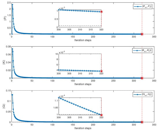
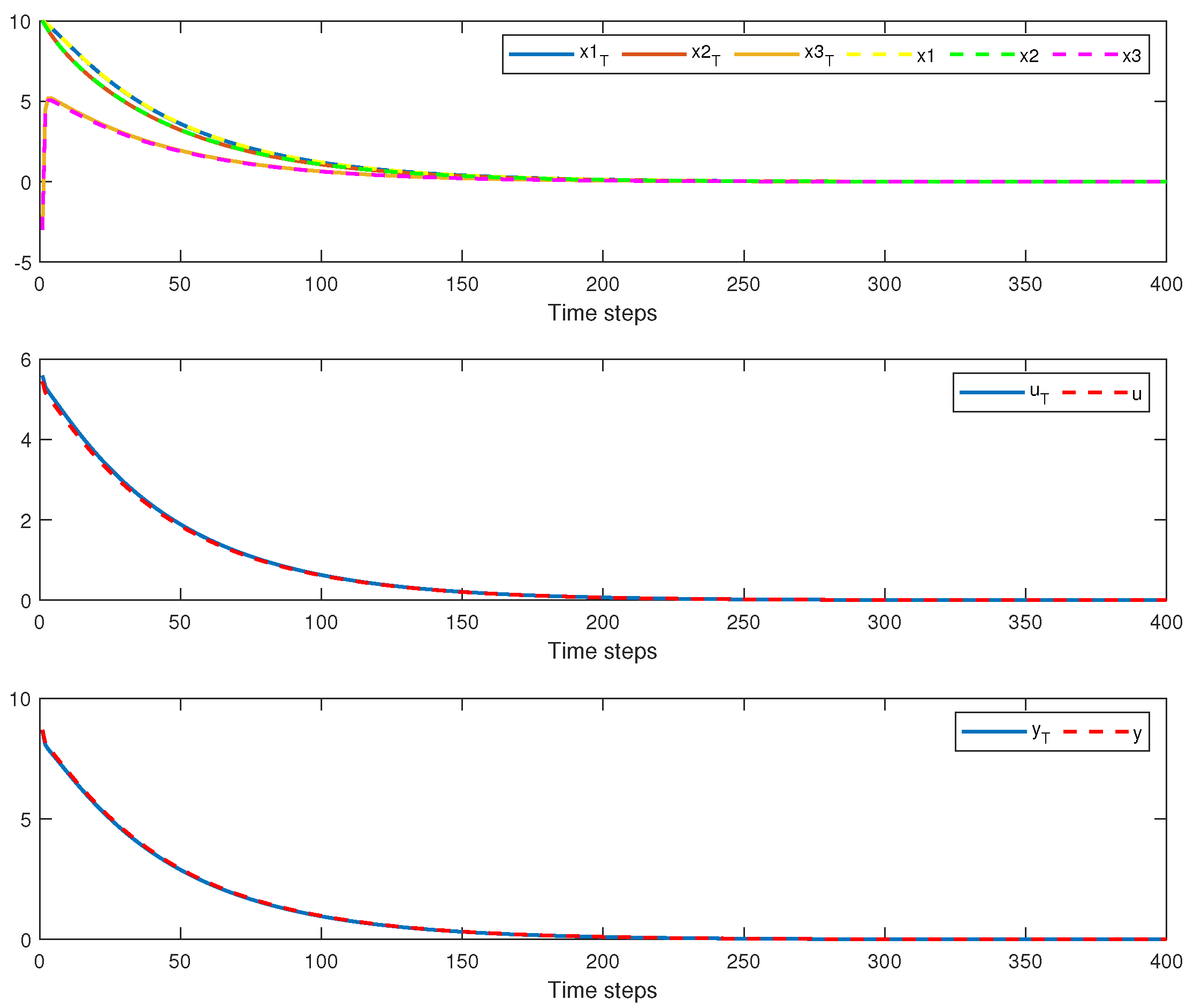
This subsection presents the results of Algorithm 1. Algorithm 1 is implemented under the condition that the system dynamics matrices A, B, and C are known, and the expert optimal feedback gain $K_T$ is available. Figure 2 illustrates the convergence performance of $P_i$, $Q_i$, and $K_i$ in Algorithm 1. It can be observed from Figure 3 that, as the number of iterations increases, the performance matrices of the learner system gradually converge. After the algorithm converges, the learned output weight is obtained as

$$Q_{\infty }=0.9142.$$

The control gain and state weighting matrix are given by

$$\left[\begin{array}{c}{K}_{\infty }=-0.4001-0.11470.0231\end{array}\right],$$

$$C^T{Q}_{\infty }C=\left[\begin{array}{ccc}0.9649& 0.09665& -0.4824\\ 0.0965& 0.0096& -0.0482\\ -0.4824& -0.0482& 0.2412\end{array}\right].$$

Specifically, the P matrix of the expert system and the $P_T$ matrix ultimately learned by the learner are

$$P=\left[\begin{array}{ccc}8.5491& 5.5134& -0.5444\\ 5.5134& 4.5822& -0.0645\\ -0.5444& -0.0645& 0.2449\end{array}\right]$$

$$P_T=\left[\begin{array}{ccc}8.7815& 5.6536& -0.5637\\ 5.6536& 4.6970& -0.0667\\ -0.5637& -0.0667& 0.2538\end{array}\right]$$

Figure 2. Convergence process of $P_i$, $K_i$ and $Q_i$ using Algorithm 1.

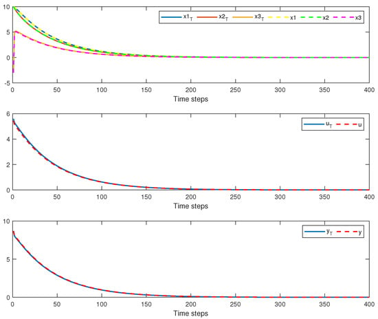
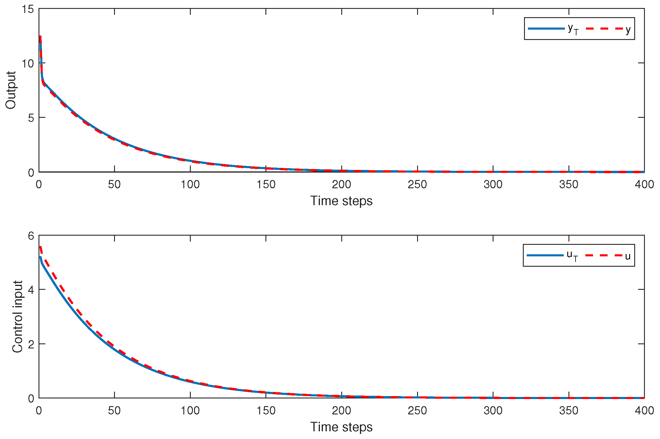
Figure 3. The learner trajectory $\left(x\right(k),u(k),y(k\left)\right)$ and expert trajectory $(x_T\left(k\right),u_T\left(k\right),y_T\left(k\right))$ for Algorithm 1.

Figure 2 shows a trajectory comparison between the expert system (2) and the learner system (1) under the same initial condition. Here, $x_T\left(k\right)$, $u_T\left(k\right)$, and $y_T\left(k\right)$ denote the state trajectory, control input trajectory, and output trajectory of the expert system (2), respectively, while $x\left(k\right)$, $u\left(k\right)$, and $y\left(k\right)$ denote those of the learner system (1).

It can be seen that, after convergence, the trajectories of the learner system (1) closely match those of the expert system (2), which verifies the effectiveness of Algorithm 1.

5.2. Simulation Results for Algorithm 2

This subsection reports the results of Algorithm 2. In contrast to Algorithm 1, Algorithm 2 operates without access to the system dynamics or state information. In the simulation, the input–output data vector $z_T\left(k\right)$ is constructed, and the state-feedback Q-function equation is transformed into the input–output form using the reconstruction relation $x_T\left(k\right)=M{z}_T\left(k\right)$.

For reproducibility, the initial output-weight matrix and the input-weight matrix are set to $Q_0=0$ and $R=1$, respectively. The batch least-squares estimation uses 43 consecutive data samples, and the algorithm is terminated when ${∥{\overline{K}}_{i+1}-{\overline{K}}_i∥}_F\le {10}^{-4}$. The common initial condition for the expert and learner systems is

$$\begin{array}{cc}\hfill x\left(0\right)& =x_T\left(0\right)={\left[\begin{array}{ccc}10& 10& -3\end{array}\right]}^T.\hfill \end{array}$$

The probing signals used for the sensitivity analysis are specified separately below, while all other simulation settings remain unchanged.

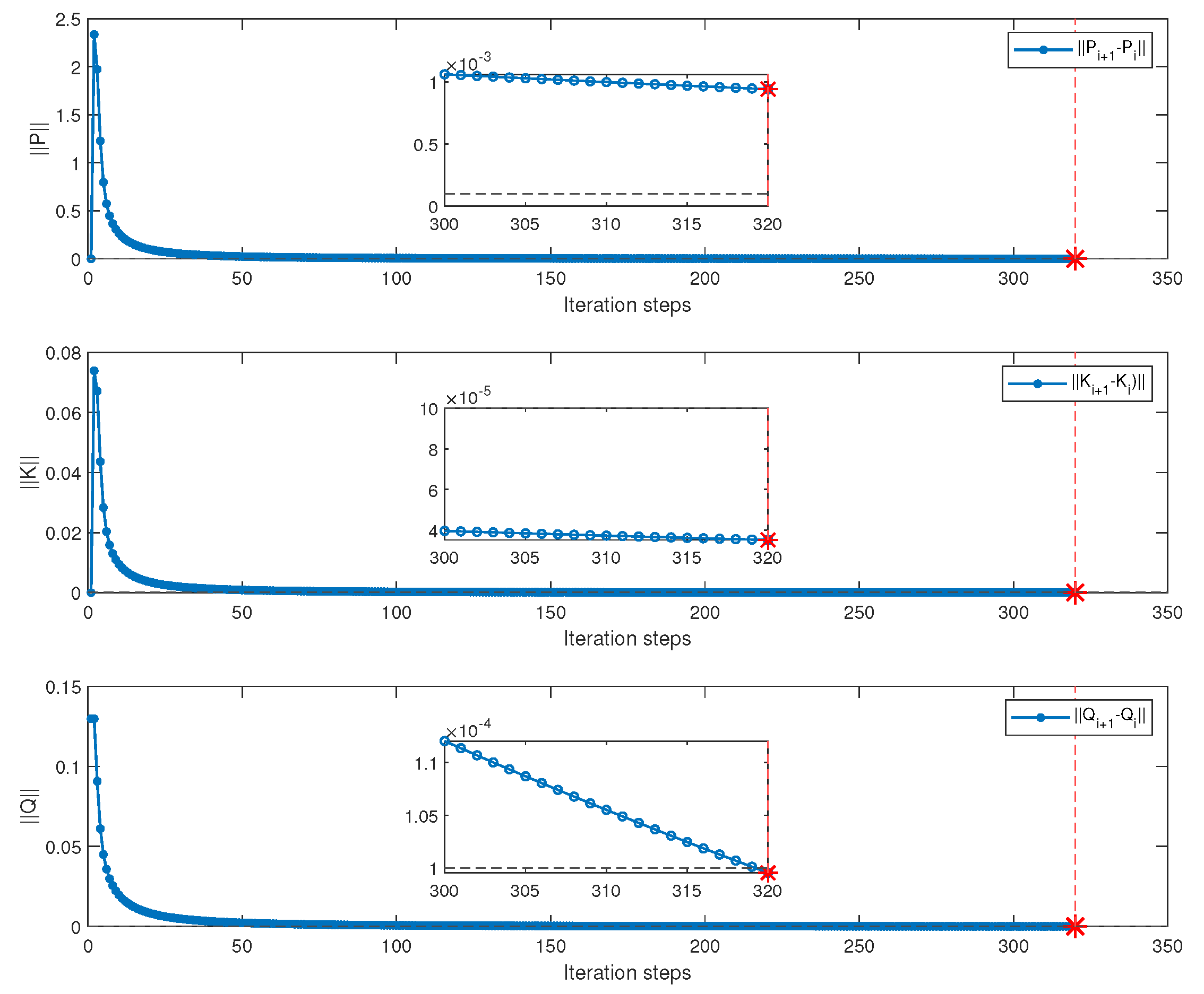
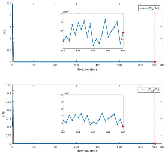
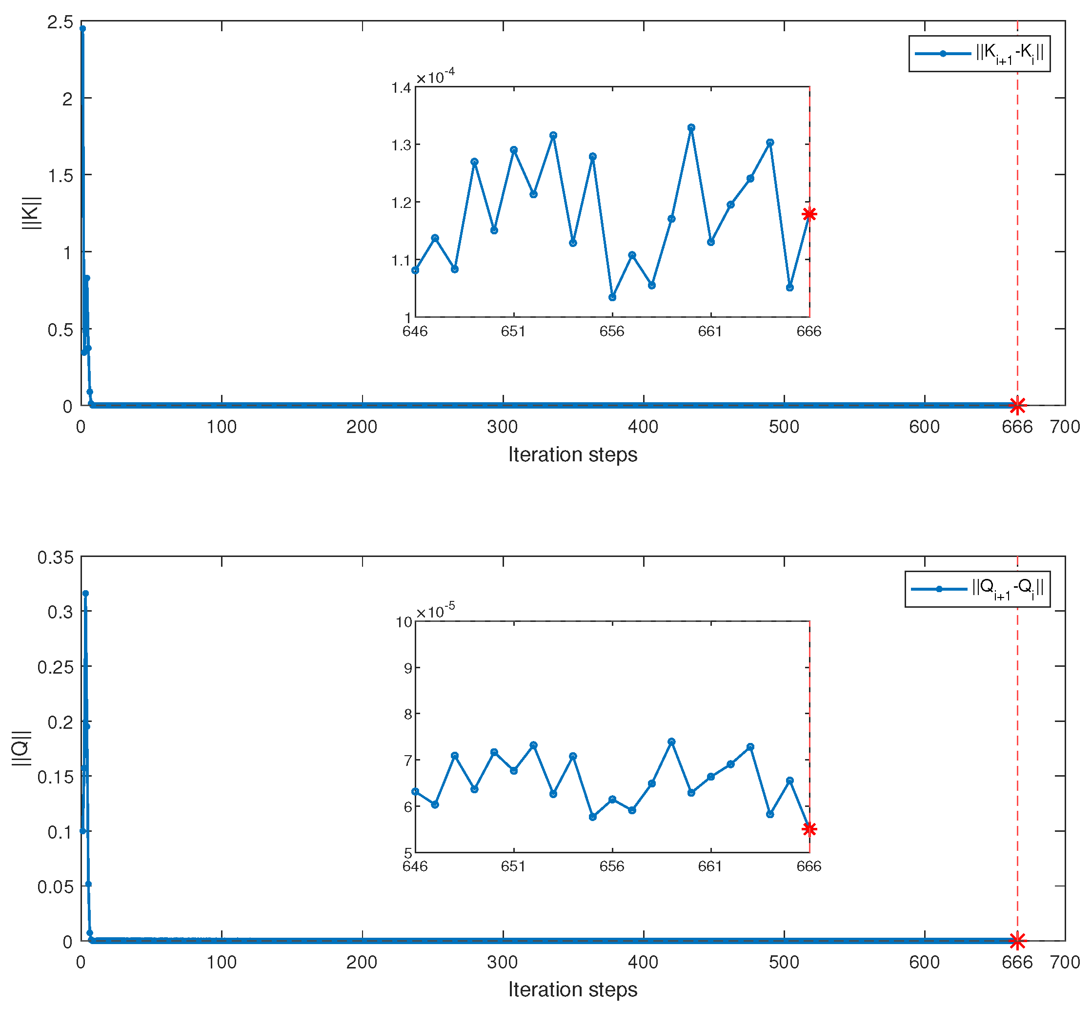
The convergence performance of $Q_i$ and ${\overline{K}}_i$ in Algorithm 2 is shown in Figure 4. The converged values of $Q_{\infty }$ and ${\overline{K}}_{\infty }$ are given by

$${\overline{K}}_{\infty }=\left[\begin{array}{c}0.0217,-0.7160,0.4800,-1.6526,-1.3257,-0.1469\end{array}\right]$$

$$Q_{\infty }=0.9142.$$

Figure 4. Convergence process of $K_i$ and $Q_i$ using Algorithm 2.

Using the state-reconstruction relation, the corresponding state-feedback control gain is obtained as

$$K_{\infty }=\left[\begin{array}{c}-0.4001,-0.1147,0.0231\end{array}\right].$$

Similarly, Figure 5 presents the trajectory comparison between the expert system (2) and the learner system (1) under Algorithm 2. Under the same initial condition, the trajectories of the learner system (1) can closely approximate those of the expert system (2). This indicates that Algorithm 2 can effectively reconstruct the performance index of the expert system without relying on a system model or state information and can learn a control policy close to that of the expert system (2).

$$\begin{array}{cc}\hfill {\overline{H}}_{xx}& =\left[\begin{array}{cccccc}0.1781& -0.6948& 0.4310& -1.6507& 1.2069& -0.1319\\ -0.6932& 134.7494& -108.5490& 309.7877& -291.5275& 33.2234\\ 0.4325& -108.5505& 87.6898& -249.5126& 235.4112& -26.8387\\ -1.6498& 309.7880& -249.5147& 712.2173& -670.1239& 76.3672\\ 1.2089& -291.5273& 235.4117& -670.1239& 632.0192& -72.0510\\ -0.1324& 33.2229& -26.8387& 76.3672& -72.0510& 8.2144\end{array}\right],\hfill \\ \hfill {\overline{H}}_{xu}& ={\overline{H}}_{ux}^T={\left[\begin{array}{cccccc}0.0256& -0.8431& 0.5651& -1.9460& 1.5610& -0.1730\end{array}\right]}^{\mathrm{T}},{\overline{H}}_{uu}=\left[\begin{array}{c}1.1775\end{array}\right]\hfill \end{array}$$

(86)

Figure 5. The learner trajectory $\left(u\right(k),y(k\left)\right)$ and expert trajectory $(u_T\left(k\right),y_T\left(k\right))$ for Algorithm 2.

The Q-function matrix partition $({\overline{H}}_{xx},{\overline{H}}_{xu},{\overline{H}}_{ux},{\overline{H}}_{uu})$ is given by (86).

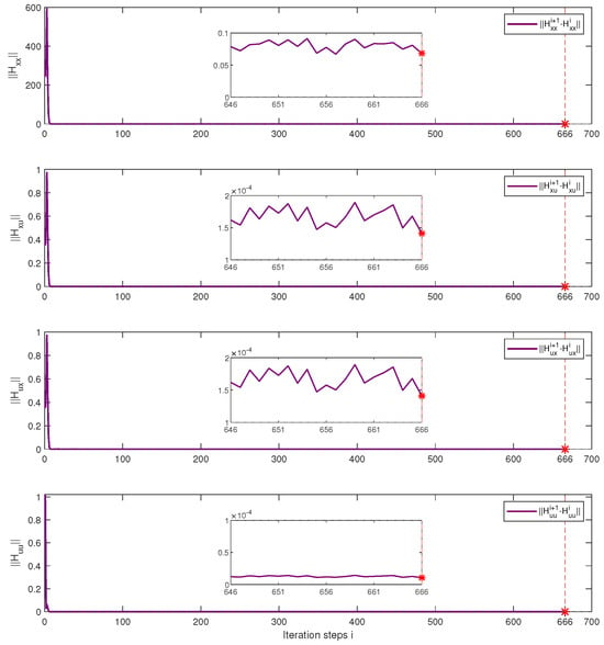
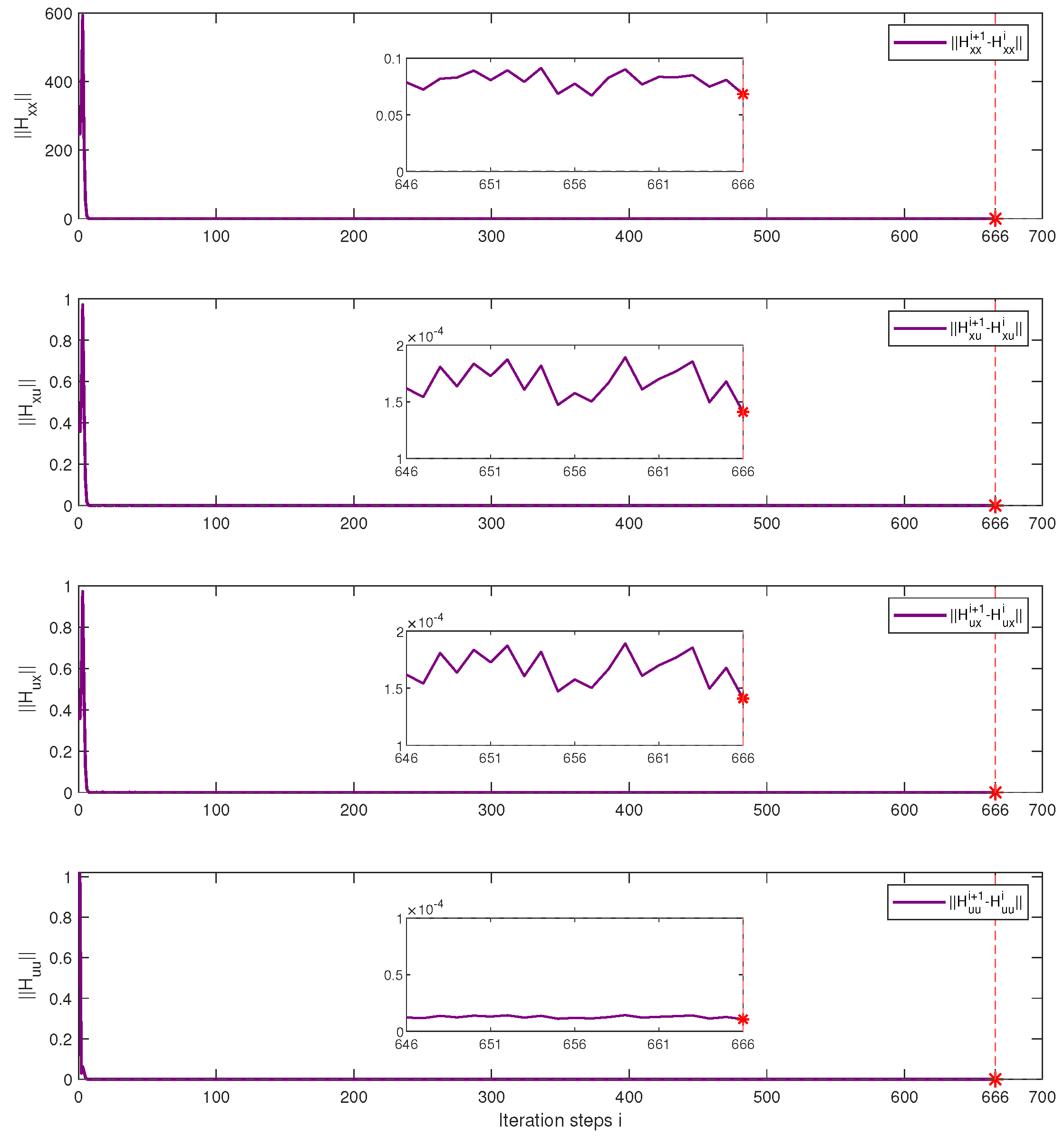
Furthermore, Figure 6 shows the convergence process of the block matrices of the input–output Q-function matrix in Algorithm 2. Specifically, the convergence errors of ${\overline{H}}_{\left(xx\right)i},{\overline{H}}_{\left(xu\right)i},{\overline{H}}_{\left(ux\right)i}$, and ${\overline{H}}_{\left(uu\right)i}$ gradually decrease and converge to a small neighbourhood of zero as the number of iterations increases. This demonstrates that the iteration process can effectively identify the Q-function matrix from the collected input–output data. Therefore, the convergence of the Q-function matrix further verifies the effectiveness and feasibility of the proposed model-free output-feedback off-policy inverse Q-learning algorithm.

Figure 6. Convergence process of ${\overline{H}}_{\left(xx\right)i},{\overline{H}}_{\left(xu\right)i},{\overline{H}}_{\left(ux\right)i}, and {\overline{H}}_{\left(uu\right)i}$ using Algorithm 2.

To investigate the influence of the probing-noise amplitude on the parameter estimation, three bounded multisine probing signals are considered:

$$\begin{array}{cc}\hfill {ϵ}_1\left(k\right)=& 0.1\sin \left(1.009k\right)+{\cos }^2\left(0.538k\right)+\sin \left(0.9k\right)+\cos \left(100k\right),\hfill \\ \hfill {ϵ}_2\left(k\right)=& 0.2\sin \left(1.009k\right)+{\cos }^2\left(0.538k\right)+\sin \left(0.9k\right)+\cos \left(100k\right),\hfill \\ \hfill {ϵ}_3\left(k\right)=& 0.3\sin \left(1.009k\right)+{\cos }^2\left(0.538k\right)+\sin \left(0.9k\right)+\cos \left(100k\right).\hfill \end{array}$$

(87)

The results in Table 1 show that Algorithm 2 converges under all three probing signals. The learned control gains remain close to the expert gain $K_T$, with gain errors of $0.0294$, $0.0303$, and $0.0304$, respectively. The iteration steps further indicate the convergence efficiency of Algorithm 2 at different probing-noise amplitudes.

Table 1. Learned control gains at different probing-noise amplitudes.

Probing Signal	Learned Control Gain ${\mathit{K}}_{\mathit{\infty }}$	$\parallel {\mathit{K}}_{\mathit{\infty }}-{\mathit{K}}_{\mathit{T}}{\parallel }_{\mathit{F}}$	Iteration Steps
${ϵ}_1\left(k\right)$	$[-0.4009,-0.1149,0.0232]$	0.0294	666
${ϵ}_2\left(k\right)$	$[-0.4001,-0.1147,0.0231]$	0.0303	666
${ϵ}_3\left(k\right)$	$[-0.3999,-0.1147,0.0231]$	0.0304	666

5.3. Comparison with the Output-Feedback RL-Based Optimal Control Method

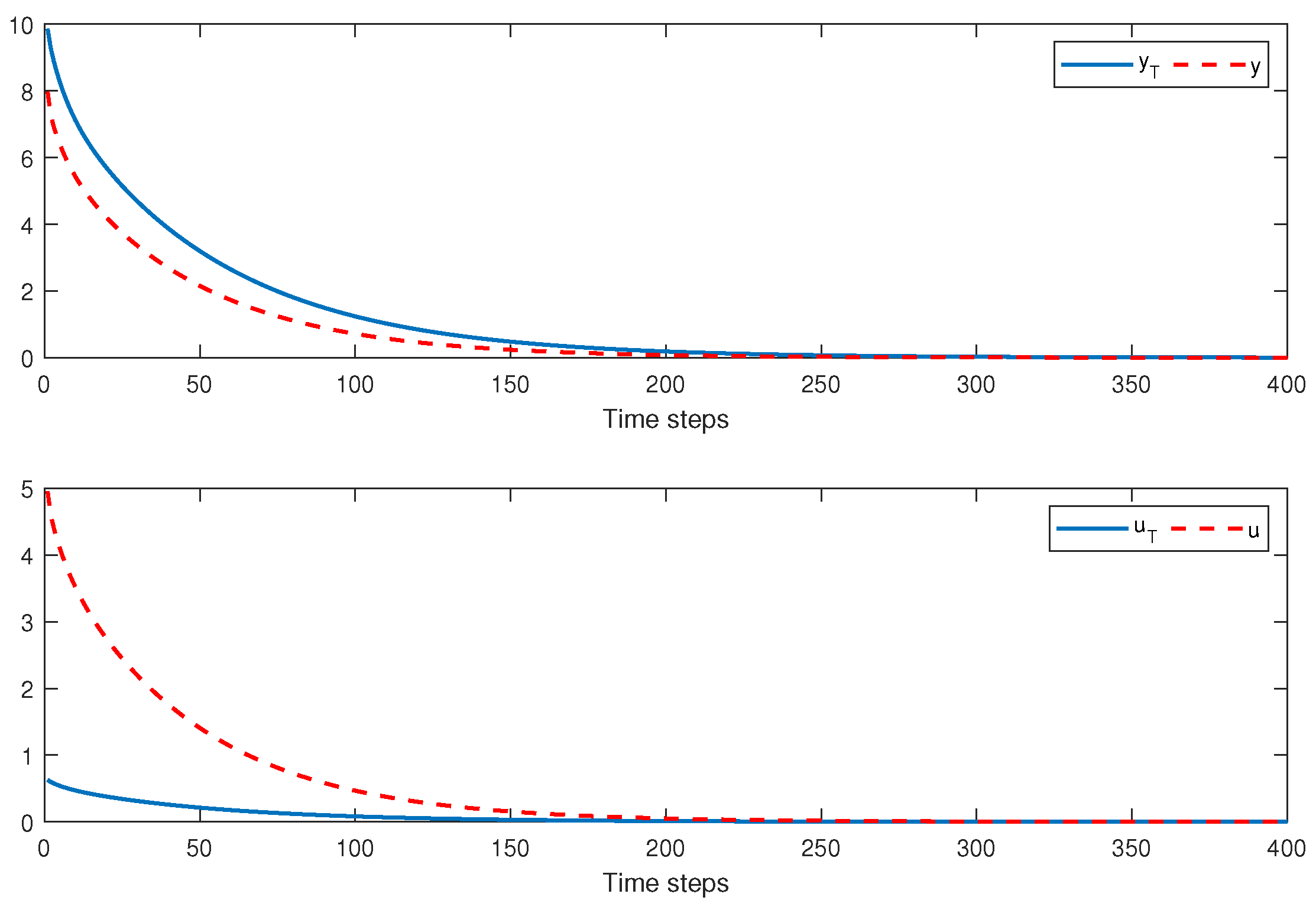
In this subsection, the F-16 aircraft system is again used as an example for algorithm comparison, where Algorithm 2 presented in this paper is compared with the DT optimal control method based on output-feedback Q-learning proposed in [35]. In that work [35], the weight matrix for the cost function (3) must be specified manually in advance. Consequently, it can only address the problem of optimal reinforcement learning control under a known cost function.

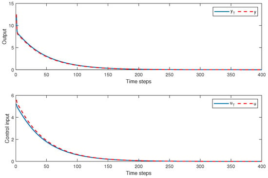
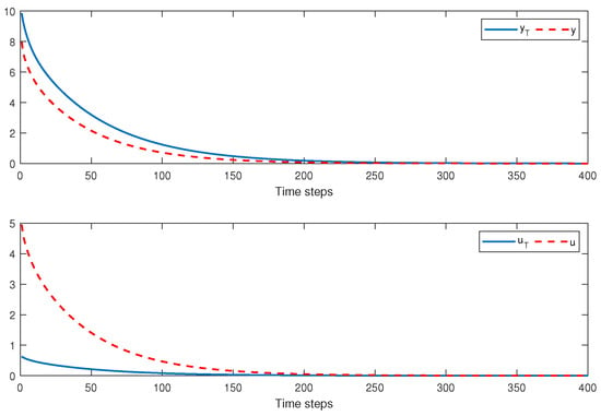
Figure 5 and Figure 7 show the comparison results between the RL-based optimal control method and our method in terms of output trajectory imitation performance. It can be observed that, using our method, the learner demonstrates superior imitation performance and is able to learn the optimal output-feedback control law without relying on system models or state information. In contrast, manually assigned cost function weights require constant adjustment, which may result in system performance failing to converge to the optimal control law as rapidly. Through imitation learning, satisfactory imitation performance can be guaranteed.

Figure 7. Simulations of the trajectories u and y were performed using an optimal control method based on RL.

To quantitatively evaluate the trajectory imitation performance, the integral absolute error (IAE) and mean square error (MSE) are calculated for both the output and control-input trajectories. Quantitative comparison of trajectory imitation performance is shown in Table 2. They are defined as

$$\begin{array}{cccc}\hfill {\mathrm{IAE}}_y& ={\displaystyle \sum _{k=1}^N}\left|y_T\left(k\right)-y\left(k\right)\right|,\hfill & \hfill {\mathrm{MSE}}_y& ={\displaystyle \frac{1}{N}}{\displaystyle \sum _{k=1}^N}{\left(y_T\left(k\right)-y\left(k\right)\right)}^2,\hfill \\ \hfill {\mathrm{IAE}}_u& ={\displaystyle \sum _{k=1}^N}\left|u_T\left(k\right)-u\left(k\right)\right|,\hfill & \hfill {\mathrm{MSE}}_u& ={\displaystyle \frac{1}{N}}{\displaystyle \sum _{k=1}^N}{\left(u_T\left(k\right)-u\left(k\right)\right)}^2.\hfill \end{array}$$

(88)

Table 2. Quantitative comparison of trajectory imitation performance.

Method	Signal	IAE	MSE
Output-feedback RL method [35]	y	141.7105	0.3605
	u	164.7927	0.7949
Proposed Algorithm 2	y	12.2063	0.0029
	u	14.1940	0.0066

6. Conclusions

This paper investigated the output-feedback inverse Q-learning problem for DT linear systems with unobservable states and proposed a data-driven output-feedback off-policy inverse Q-learning algorithm. First, a model-based IRL algorithm was presented as the basic framework. Building on this framework, a model-free output-feedback IRL algorithm was developed using only expert input–output trajectory data and without requiring a system model. Theoretical analysis demonstrated that the proposed algorithm achieves convergence and closed-loop stability under appropriate conditions. Finally, the effectiveness of the proposed algorithm was verified through simulation examples, with results indicating that the learner can closely approximate the cost function structure and control performance of the expert system.

Compared with existing IRL methods, the approach has overcome the reliance of traditional state-feedback methods on the measurability of system states, enabling inverse Q-learning to be applied in output-feedback scenarios where states cannot be directly measured. Future work may further consider extending the proposed method to more general nonlinear systems and multi-agent game scenarios, conducting experimental validation on actual control objects, and combining robust data-estimation and $H_{\infty }$ control techniques with the proposed framework to improve its robustness against measurement noise and model uncertainties.

References

- Lewis, F.L.; Vrabie, D.; Syrmos, V.L. Optimal Control; John Wiley & Sons: Hoboken, NJ, USA, 2012. [Google Scholar]
- Zhao, D.B.; Shao, K.; Zhu, Y.H.; Li, D.; Chen, Y.R.; Wang, H.T.; Liu, D.R.; Zhou, T.; Wang, C.H. Review of deep reinforcement learning and discussions on the development of computer Go. Kongzhi Lilun Yu Yingyong/Control Theory Appl. 2016, 33, 701–717. [Google Scholar]
- Zhang, H.G.; Zhang, X.; Yan-Hong, L.; Jun, Y. An overview of research on adaptive dynamic programming. Acta Autom. Sin. 2013, 39, 303–311. [Google Scholar] [CrossRef] [Scilit]
- Abbeel, P.; Ng, A.Y. Apprenticeship learning via inverse reinforcement learning. In Proceedings of the Twenty-first International Conference on Machine Learning, Banff, AB, Canada, 4–8 July 2004; p. 1. [Google Scholar]
- Zhifei, S.; Joo, E.M. A review of inverse reinforcement learning theory and recent advances. In Proceedings of the 2012 IEEE Congress on Evolutionary Computation; IEEE: Piscataway, NJ, USA, 2012; pp. 1–8. [Google Scholar]
- Ng, A.Y.; Russell, S. Algorithms for inverse reinforcement learning. In Proceedings of the Icml, Stanford, CA, USA, 29 June–2 July 2000; Volume 1, p. 2. [Google Scholar]
- Ab Azar, N.; Shahmansoorian, A.; Davoudi, M. From inverse optimal control to inverse reinforcement learning: A historical review. Annu. Rev. Control 2020, 50, 119–138. [Google Scholar] [CrossRef] [Scilit]
- Self, R.; Abudia, M.; Kamalapurkar, R. Online inverse reinforcement learning for systems with disturbances. In Proceedings of the 2020 American Control Conference (ACC); IEEE: Piscataway, NJ, USA, 2020; pp. 1118–1123. [Google Scholar]
- Xue, W.; Lian, B.; Fan, J.; Chai, T.; Lewis, F.L. Inverse reinforcement learning for trajectory imitation using static output feedback control. IEEE Trans. Cybern. 2023, 54, 1695–1707. [Google Scholar] [CrossRef] [Scilit] [PubMed]
- Lian, B.; Xue, W.; Lewis, F.L.; Davoudi, A. Inverse Q-learning using input–output data. IEEE Trans. Cybern. 2023, 54, 728–738. [Google Scholar] [CrossRef] [Scilit] [PubMed]
- Wu, Z.; Sun, L.; Zhan, W.; Yang, C.; Tomizuka, M. Efficient sampling-based maximum entropy inverse reinforcement learning with application to autonomous driving. IEEE Robot. Autom. Lett. 2020, 5, 5355–5362. [Google Scholar] [CrossRef] [Scilit]
- Lian, B.; Xue, W.; Lewis, F.L.; Chai, T. Inverse reinforcement learning for adversarial apprentice games. IEEE Trans. Neural Netw. Learn. Syst. 2021, 34, 4596–4609. [Google Scholar] [CrossRef] [Scilit] [PubMed]
- Cao, K.; Xie, L. Game-theoretic inverse reinforcement learning: A differential pontryagin’s maximum principle approach. IEEE Trans. Neural Netw. Learn. Syst. 2022, 34, 9506–9513. [Google Scholar] [CrossRef] [Scilit] [PubMed]
- Self, R.; Abudia, M.; Mahmud, S.N.; Kamalapurkar, R. Model-based inverse reinforcement learning for deterministic systems. Automatica 2022, 140, 110242. [Google Scholar] [CrossRef] [Scilit]
- Liu, W.; Wu, R.; Si, J.; Huang, H. A new robotic knee impedance control parameter optimization method facilitated by inverse reinforcement learning. IEEE Robot. Autom. Lett. 2022, 7, 10882–10889. [Google Scholar] [CrossRef] [Scilit]
- Xue, W.; Kolaric, P.; Fan, J.; Lian, B.; Chai, T.; Lewis, F.L. Inverse reinforcement learning in tracking control based on inverse optimal control. IEEE Trans. Cybern. 2021, 52, 10570–10581. [Google Scholar] [CrossRef] [Scilit] [PubMed]
- Self, R.; Coleman, K.; Bai, H.; Kamalapurkar, R. Online observer-based inverse reinforcement learning. IEEE Control Syst. Lett. 2020, 5, 1922–1927. [Google Scholar] [CrossRef] [Scilit]
- Clarke, S.G.; Byeon, S.; Hwang, I. A low complexity approach to model-free stochastic inverse linear quadratic control. IEEE Access 2022, 10, 9298–9308. [Google Scholar] [CrossRef] [Scilit]
- Lian, B.; Kartal, Y.; Lewis, F.L.; Mikulski, D.G.; Hudas, G.R.; Wan, Y.; Davoudi, A. Anomaly detection and correction of optimizing autonomous systems with inverse reinforcement learning. IEEE Trans. Cybern. 2022, 53, 4555–4566. [Google Scholar] [CrossRef] [Scilit] [PubMed]
- Choi, S.; Kim, S.; Jin Kim, H. Inverse reinforcement learning control for trajectory tracking of a multirotor UAV. Int. J. Control Autom. Syst. 2017, 15, 1826–1834. [Google Scholar] [CrossRef] [Scilit]
- Ho, J.; Ermon, S. Generative adversarial imitation learning. Adv. Neural Inf. Process. Syst. 2016, 29, 4565–4573. [Google Scholar]
- Lian, B.; Xue, W.; Xie, Y.; Lewis, F.L.; Davoudi, A. Off-policy inverse Q-learning for discrete-time antagonistic unknown systems. Automatica 2023, 155, 111171. [Google Scholar] [CrossRef] [Scilit]
- Zhao, Z.; Wang, T.; Peng, F.; Yu, J. Adaptive Fuzzy Resilient Decentralized Control for Nonlinear Large-Scale CPSs Under DoS Attacks. IEEE Trans. Fuzzy Syst. 2024, 32, 5899–5909. [Google Scholar] [CrossRef] [Scilit]
- Zhao, Z.; Wang, T.; Yu, J.; Basin, M.V. Bilateral Cooperative Control of Nonlinear Multiagent Systems With State and Output Quantification. IEEE Trans. Cybern. 2025, 55, 2949–2957. [Google Scholar] [CrossRef] [Scilit] [PubMed]
- Xue, W.; Lian, B.; Kartal, Y.; Fan, J.; Chai, T.; Lewis, F.L. Model-free inverse H-infinity control for imitation learning. IEEE Trans. Autom. Sci. Eng. 2024, 22, 5661–5672. [Google Scholar] [CrossRef] [Scilit]
- Lian, B.; Xue, W.; Lewis, F.L.; Chai, T. Inverse reinforcement learning for multi-player noncooperative apprentice games. Automatica 2022, 145, 110524. [Google Scholar] [CrossRef] [Scilit]
- Wu, H.; Hu, Q.; Zheng, J.; Dong, F.; Ouyang, Z.; Li, D. Discounted Inverse Reinforcement Learning for Linear Quadratic Control. IEEE Trans. Cybern. 2025, 55, 1995–2007. [Google Scholar] [CrossRef] [Scilit] [PubMed]
- Xue, W.; Lian, B.; Fan, J.; Kolaric, P.; Chai, T.; Lewis, F.L. Inverse reinforcement Q-learning through expert imitation for discrete-time systems. IEEE Trans. Neural Netw. Learn. Syst. 2021, 34, 2386–2399. [Google Scholar] [CrossRef] [Scilit] [PubMed]
- Lian, B.; Donge, V.S.; Lewis, F.L.; Chai, T.; Davoudi, A. Data-driven inverse reinforcement learning control for linear multiplayer games. IEEE Trans. Neural Netw. Learn. Syst. 2022, 35, 2028–2041. [Google Scholar] [CrossRef] [Scilit] [PubMed]
- Bittanti, S.; Laub, A.J.; Willems, J.C. The Riccati Equation; Springer: Berlin/Heidelberg, Germany, 1991; pp. 131–162. [Google Scholar]
- Li, J.; Yuan, D.; Ding, Z. Optimal tracking control for discrete-time systems by model-free off-policy Q-learning approach. In Proceedings of the 2017 11th Asian Control Conference (ASCC); IEEE: Piscataway, NJ, USA, 2017; pp. 7–12. [Google Scholar]
- Al-Tamimi, A.; Lewis, F.L.; Abu-Khalaf, M. Model-free Q-learning designs for linear discrete-time zero-sum games with application to H-infinity control. Automatica 2007, 43, 473–481. [Google Scholar] [CrossRef] [Scilit]
- Kiumarsi, B.; Lewis, F.L.; Jiang, Z.P. H-infinity control of linear discrete-time systems: Off-policy reinforcement learning. Automatica 2017, 78, 144–152. [Google Scholar] [CrossRef] [Scilit]
- Lewis, F.L.; Vamvoudakis, K.G. Reinforcement learning for partially observable dynamic processes: Adaptive dynamic programming using measured output data. IEEE Trans. Syst. Man Cybern. Part B (Cybern.) 2010, 41, 14–25. [Google Scholar] [CrossRef] [Scilit] [PubMed]
- Rizvi, S.A.A.; Lin, Z. Output Feedback Q-Learning Control for the Discrete-Time Linear Quadratic Regulator Problem. IEEE Trans. Neural Netw. Learn. Syst. 2019, 30, 1523–1536. [Google Scholar] [CrossRef] [Scilit] [PubMed]
Disclaimer/Publisher’s Note: The statements, opinions and data contained in all publications are solely those of the individual author(s) and contributor(s) and not of MDPI and/or the editor(s). MDPI and/or the editor(s) disclaim responsibility for any injury to people or property resulting from any ideas, methods, instructions or products referred to in the content. |
© 2026 by the authors. Licensee MDPI, Basel, Switzerland. This article is an open access article distributed under the terms and conditions of the Creative Commons Attribution (CC BY) license.