Control of Linear Time-Delay Actuators Based on Virtual Reference Trajectory

Abstract

A control approach for linear actuators with time delay is introduced. The novelty of the proposal is the inclusion of a virtual reference trajectory (VRT) without modifying the controller architecture, allowing the stability margin of a single-delay actuator controller to be increased; in the ideal case, the proposed approach can render stability independent of delay. Moreover, a slight modification of the dynamics of the virtual trajectory allows the closed-loop system to be expressed as a neutral time-delay system. Therefore, its stability analysis is performed using the Lyapunov–Krasovskii approach, yielding theoretical conditions that allow the critical time delay to be computed. Numerical simulations and experiments on the control of a DC motor actuator with a control input time delay validate our proposal.

1. Introduction

Control systems in daily activities are ubiquitous [1] and are usually affected by several endogenous and exogenous uncertainties and disturbances. In more complex situations, time delays—either in the control, in the state, or in the output measurement of the system—are also important aspects to be considered [2]. The combined effect of disturbances and time delay is, most of the time, detrimental to controller performance. Additionally, the control of systems with time delay is challenging, given the different types of delays arising in practical and theoretical applications [3,4,5,6]. Several approaches to address this problem are found in the literature; see Table 1.

Table 1. Comparative table of main time-delay control/compensation schemes.

Approach	References	Required Time-Delay Knowledge	Model-Dependence	Implementation-Computational Complexity
Predictors	[7,8,9]	Known/Exact	High	Moderate
Observers	[10,11,12]	Known/Bounded	High	Moderate
Passivity-based	[13,14,15]	Bounded	Moderate	Low
Backstepping	[16,17]	Known/Bounded	High	High
Artificial intelligence	[18,19]	Unknown	Low	High

The research extending the Lyapunov approach to time-delay system stability was first successfully implemented by Krasovskii [20] while Razumikhin proposed an alternative framework shortly thereafter [3]. More recently, proposals in this context have been developed [21]. To further analyze the stability of time-delay systems, the study of Lyapunov–Krasovskii functionals has led to the establishment of delay-independent conditions in terms of linear matrix inequalities (LMIs) where unknown matrices appear linearly in the inequality to guarantee stability, which can therefore be efficiently computed using convex optimization techniques [22,23,24]. In contrast, when controller synthesis is incorporated into the stability analysis, products between the controller gains and the Lyapunov matrices naturally arise, leading to bilinear matrix inequalities (BMIs), whose numerical solution is considerably more challenging [25]. As for their numerical resolution, it can be mentioned that only in some cases is it possible to convert these BMIs into a set of LMIs that can be solved with semidefinite programming [26]. For delay-free control systems, when time delays appear, stability and stabilization are considered major issues [27]. Although stable linear systems generally exhibit a certain degree of robustness to small delays, maintaining stability and satisfactory performance under increasing delays remains a major challenge. In this context, existing delay-compensation methods frequently rely on time-delay knowledge, plant-dependent prediction models, or observer-based structures, thus yielding medium to high model dependency and/or implementation complexity, as shown in Table 1. These requirements complicate implementation and reduce robustness under delay uncertainty. The proposed approach addresses these limitations threefold:

• Eliminates the need for explicit delay knowledge or prediction, in the ideal case rendering stability independent of the time delay and thus improving robustness to time-delay uncertainty.
• Enlarges the admissible delay margin while preserving the original controller architecture, reducing implementation complexity.
• Introduces a low-order VRT generator that reconstructs delayed tracking information directly from measured delayed errors, reducing model dependency.

In a wide range of control systems, sensors and actuators are fundamental to ensuring the main goals of any control system: stability and performance. One of the most common actuators in control systems is the DC motor [28,29]. Those actuators are affected by several endogenous and exogenous uncertainties and disturbances, including time delays; therefore, different approaches have been reported. Delay estimation and predictive control schemes have been used for theoretical studies and experimental validation on DC motors [30]. The speed control of a DC motor based on a wireless networked control system with time-delay and saturation parameters was experimentally studied in [31]. Dharshan [32] explored the use of the classic Smith predictor (SP) using a direct structure networked control system; his results were obtained for a total network delay greater than 1 [s]. The speed control of a DC motor with input delay and external disturbance was investigated using $H_{\infty }$ control, with the results compared with those of a PID controller, demonstrating usefulness and efficiency [33]. Stability analysis and the computation of the stability delay margin for robust DC motor control have recently been studied in [34,35]. Moreover, the tradeoff between stability and performance for DC motor actuators in control systems with single time delays is studied in [36].

The main contribution of this work lies in a novel method consisting of the consideration of the VRT dynamics in the state feedback controller to achieve accurate tracking while ensuring closed-loop stability. A similar idea is used in the force control of robotic systems within the impedance/admittance control approach [37,38]. In this force control approach, the robot’s desired trajectory is modified online to achieve the desired force. The main idea is to compute online an additional reference trajectory, which is then added to the desired trajectory in order to achieve force tracking. To better describe our proposal, we first assume that the linear system is either stable or stabilized by a feedback control law [39]. Then, by incorporating the proposed VRT dynamics into the feedback controller, specifically by adding it to the desired trajectory within the time-delay error, stability can be ensured through proper tuning of the parameters. The VRT is generated by an adjoint linear dynamical system driven by the time-delay tracking error and its time derivatives. The resulting system is a standard linear neutral time-delay system whose stability can be rigorously analyzed using state-of-the-art results. It is important to highlight that the interpretation of VRT means that it represents a trajectory computed online. In the following, we refer to a VRT or reference trajectory in the same way.

The rest of the paper is organized as follows. Section 2 describes the mathematical models considered, presenting the motivation of our proposal using a second-order linear system. In Section 3, the problem statement, the generalization of the proposed approach, the study of its stability, and a numerical simulation to validate the theoretical findings are detailed. Section 4 presents numerical simulations comparing our approach with the classic SP and results on a DC motor testbed to experimentally validate our proposal. Finally, conclusions and some research directions are provided in Section 5.

2. Introductory Mathematical Models

In this section, the motivation of the proposed approach is described using a second-order dynamical system as an introductory example. The proposed VRT dynamics are presented to express the system in standard neutral form.

2.1. Motivation

Consider the linear system:

$$\ddot{x}+a_1\dot{x}+a_{0}x=b_0{u}_{\tau },$$

(1)

where $x\in \mathbb{R}$ represents a state position of the system with its corresponding time derivatives $\dot{x}$ and $\ddot{x}$; $a_0$, $a_1$ and $b_0$ are scalar constant parameters, and $u_{\tau }$ is the controller defined as follows:

$$u_{\tau }=u(t-\tau )={\displaystyle \frac{1}{b_0}}\left({\ddot{x}}_d+a_1{\dot{x}}_d+a_0{x}_d-K_0(x_{\tau }-x_{d_{\tau }}-x_r)-K_1({\dot{x}}_{\tau }-{\dot{x}}_{d_{\tau }}-{\dot{x}}_r)\right),$$

(2)

where $\tau$ stands for the time delay, $x_{\tau }=x(t-\tau )$ is the delayed output, $x_{d_{\tau }}\left(t\right)$ is the delayed desired trajectory and $x_r\left(t\right)$ is a reference trajectory to be computed online in order to compensate for the time-delay errors, $x_d$ represents the desired trajectory, and $K_0$ and $K_1$ are scalar gains. Notice that the desired trajectory is always available, so it can be used for direct feedforward and in the delay-time error computation. Considering (1) and (2), the closed-loop equation is as follows:

$$(\ddot{x}-{\ddot{x}}_d)+a_1(\dot{x}-{\dot{x}}_d)+a_0(x-x_d)=-K_0(x_{\tau }-x_{d_{\tau }}-x_r)-K_1({\dot{x}}_{\tau }-{\dot{x}}_{d_{\tau }}-{\dot{x}}_r).$$

(3)

Define the tracking error $e=x-x_d$ and the delayed tracking error $e_{\tau }=x_{\tau }-x_{d_{\tau }}$. Then, Equation (3) can be rewritten as follows:

$$\ddot{e}+a_1\dot{e}+a_{0}e=-K_0(e_{\tau }-x_r)-K_1({\dot{e}}_{\tau }-{\dot{x}}_r).$$

(4)

From Equation (4), to render asymptotic closed-loop stability of the tracking error e, a natural selection for the reference dynamics is chosen as follows:

$$K_1{\dot{x}}_r=-K_0{x}_r+K_0{e}_{\tau }+K_1{\dot{e}}_{\tau }.$$

(5)

If $K_0>0$, the reference trajectory represents a stable first-order linear system for $x_r$, perturbed by a term dependent on the delayed tracking error and its time derivative. In this ideal case, as will be shown later, the proposed controller yields stability independent of delay [40].

2.2. Reference Trajectory Modification

Let $z\left(t\right)={[e,\dot{e},x_r]}^T$ and $z(t-\tau )={[e_{\tau },{\dot{e}}_{\tau },x_r]}^T$. Consider the reference trajectory of Equation (5) modified with a tunable gain ${\delta }_0>0$ as in Equation (6).

$$K_1{\dot{x}}_r=-{\delta }_0{K}_0{x}_r+K_0{e}_{\tau }+K_1{\dot{e}}_{\tau }.$$

(6)

Notice that Equation (6) is implementable provided the delayed error $e_{\tau }$ is an available signal even for $t<\tau$. Thus, it is important to highlight that the reference trajectory is not delayed in the definition of $z(t-\tau )$.

On the one hand, considering Equations (4) and (6), the closed loop is obtained as follows:

$$\begin{array}{c}\hfill \ddot{e}+a_1\dot{e}+a_{0}e=-K_0{e}_{\tau }+K_0{x}_r-K_1{\dot{e}}_{\tau }-{\delta }_0{K}_0{x}_r+K_0{e}_{\tau }+K_1{\dot{e}}_{\tau }.\end{array}$$

(7)

In this case, perfect cancellation of the delayed terms is achieved, yielding the following:

$$\begin{array}{c}\hfill \ddot{e}+a_1\dot{e}+a_{0}e=K_0(1-{\delta }_0)x_r,\end{array}$$

(8)

clearly, when ${\delta }_0=1$, the delay has no effect, and the tracking error converges asymptotically to zero.

On the other hand, Equations (4) and (6) can be written to represent a neutral time-delay difference equation in standard form:

$$E\dot{z}\left(t\right)={\overline{A}}_{0}z\left(t\right)+{\overline{A}}_{1}z(t-\tau ),$$

(9)

where

$$\begin{array}{cccc}E=\left[\begin{array}{ccc}1& 0& 0\\ 0& 1& -K_1\\ 0& 0& K_1\end{array}\right],& {\overline{A}}_0=\left[\begin{array}{ccc}0& 1& 0\\ -a_0& -a_1& K_0\\ 0& 0& -{\delta }_0{K}_0\end{array}\right]& \mathrm{and}& {\overline{A}}_1=\left[\begin{array}{ccc}0& 0& 0\\ -K_0& -K_1& 0\\ K_0& K_1& 0\end{array}\right]\end{array}$$

Given that $K_1\ne 0$, it is clear that the matrix E is invertible and (9) can be written as a single-delay equation:

$$\dot{z}\left(t\right)={\overline{A}}_{0}z\left(t\right)+{\overline{A}}_{1}z(t-\tau ),$$

(10)

where

$$\begin{array}{ccc}{A}_0=E^{-1}{\overline{A}}_0=\left[\begin{array}{ccc}0& 1& 0\\ -a_0& -a_1& K_0(1-{\delta }_0)\\ 0& 0& -{\delta }_0{\displaystyle \frac{K_0}{K_1}}\end{array}\right]& \mathrm{and}& A_1=E^{-1}{\overline{A}}_1=\left[\begin{array}{ccc}0& 0& 0\\ 0& 0& 0\\ {\displaystyle \frac{K_0}{K_1}}& 1& 0\end{array}\right]\end{array}$$

Remark 1.

When ${\delta }_0=1$, it can be verified that Equation (10) is exponentially stable independent of delay, provided that $det(sI-A_0-A_1{e}^{-s\tau })\ne 0$ for all τ, [3].

3. Problem Statement and Generalization

This section describes the problem statement and generalization of the proposed approach. Then, the stability analysis is performed, and finally, in order to demonstrate the usefulness of the theoretical analysis, a set of simulations considering a linear actuator is presented.

Consider the linear dynamical system:

$$x^{\left(n\right)}+a_{n-1}{x}^{(n-1)}+\dots +a_2\ddot{x}+a_1\dot{x}+a_{0}x=b_{0}u.$$

(11)

In this case, the controller is proposed as follows:

$$u(t-\tau )={\displaystyle \frac{1}{b_0}}\left(x_d^{\left(n\right)}+{\displaystyle \sum _{i=0}^{n-1}}{a}_i{x}_d^{\left(i\right)}-{\displaystyle \sum _{i=0}^{n-1}}{K}_i\left(e_{\tau }^{\left(i\right)}-x_r^{\left(i\right)}\right)\right),$$

(12)

where

$$e_{\tau }^{\left(i\right)}={\displaystyle \frac{d^{\left(i\right)}}{d{t}^{\left(i\right)}}}e(t-\tau )={\displaystyle \frac{d^{\left(i\right)}}{d{t}^{\left(i\right)}}}(x_{\tau }-x_{d_{\tau }}).$$

(13)

Problem 1.

Compute a virtual reference trajectory $x_r$, which renders the closed-loop system (11) and (12) stable, guaranteeing that ${lim}_{t\to \infty }e\left(t\right)=0$.

In order to solve the above problem, we proceed as in Section 2. Substituting the controller (12) into the system (11) yields the closed-loop equation:

$$e^{\left(n\right)}+{\displaystyle \sum _{i=0}^{n-1}}{a}_i{e}^{\left(i\right)}=-{\displaystyle \sum _{i=0}^{n-1}}{K}_i(e_{\tau }^{\left(i\right)}-x_r^{\left(i\right)});$$

(14)

now, isolating the $(n-1)$th time derivative of the reference trajectory:

$$e^{\left(n\right)}+{\displaystyle \sum _{i=0}^{n-1}}{a}_i{e}^{\left(i\right)}=-{\displaystyle \sum _{i=0}^{n-1}}{K}_i{e}_{\tau }^{\left(i\right)}+{\displaystyle \sum _{i=0}^{n-2}}{K}_i{x}_r^{\left(i\right)}+K_{n-1}{x}_r^{(n-1)}.$$

(15)

The modified dynamics of the reference trajectory are set as follows:

$$K_{n-1}{x}_r^{(n-1)}=-{\displaystyle \sum _{i=0}^{n-2}}{\delta }_i{K}_i{x}_r^{\left(i\right)}+{\displaystyle \sum _{i=0}^{n-1}}{K}_i{e}_{\tau }^{\left(i\right)}.$$

(16)

Defining the state $z\left(t\right)\in {\mathbb{R}}^{(2n-1)}$ as

$$\begin{array}{ccc}\hfill z\left(t\right)& =& \left[\begin{array}{c}e\\ \dot{e}\\ ⋮\\ e^{(n-1)}\\ x_r\\ {\dot{x}}_r\\ ⋮\\ x_r^{(n-2)}\end{array}\right],\hfill \end{array}$$

(17)

the system (15), when considered in closed loop with the reference trajectory (16), can be written as a single time-delay system:

$$\mathbf{E}\dot{z}\left(t\right)={\overline{\mathbf{A}}}_{0}z\left(t\right)+{\overline{\mathbf{A}}}_{1}z(t-\tau )$$

(18)

where

$$\mathbf{E}=\left[\begin{array}{cccc}{I}_{(n-1)\times (n-1)}& 0_{(n-1)\times \left(1\right)}& 0_{(n-1)\times (n-2)}& 0_{(n-1)\times \left(1\right)}\\ 0_{\left(1\right)\times (n-1)}& 1& 0_{\left(1\right)\times (n-2)}& -K_{n-1}\\ 0_{(n-2)\times (n-1)}& 0_{(n-2)\times \left(1\right)}& I_{(n-2)\times (n-2)}& 0_{(n-2)\times \left(1\right)}\\ 0_{\left(1\right)\times (n-1)}& 0& 0_{\left(1\right)\times (n-2)}& K_{n-1}\end{array}\right]$$

$${\overline{\mathbf{A}}}_0=\left[\begin{array}{cccc}{0}_{(n-1)\times \left(1\right)}& I_{(n-1)\times (n-1)}& 0_{(n-1)\times \left(1\right)}& 0_{(n-1)\times (n-2)}\\ -a_0& -\left[a_1,\dots ,a_{n-1}\right]& K_0& \left[K_1,\dots ,K_{n-2}\right]\\ 0_{(n-2)\times \left(1\right)}& 0_{(n-2)\times (n-1)}& 0_{(n-2)\times \left(1\right)}& I_{(n-2)\times (n-2)}\\ 0& 0_{\left(1\right)\times (n-1)}& -{\delta }_0{K}_0& -[{\delta }_1{K}_1,\dots ,{\delta }_{n-2}{K}_{n-2}]\end{array}\right]$$

$${\overline{\mathbf{A}}}_1=\left[\begin{array}{cc}{0}_{(n-1)\times \left(n\right)}& 0_{(n-1)\times (n-1)}\\ -[K_0,\dots ,K_{n-1}]& 0_{\left(1\right)\times (n-1)}\\ 0_{(n-2)\times \left(n\right)}& 0_{(n-2)\times (n-1)}\\ \left[K_0,\dots ,K_{n-1}\right]& 0_{\left(1\right)\times (n-1)}\end{array}\right].$$

The above matrices are of size $(2n-1)$. Then, by induction, we obtain

$${\mathbf{E}}_n^{-1}=\left[\begin{array}{cccc}{I}_{(n-1)\times (n-1)}& 0_{(n-1)\times \left(1\right)}& 0_{(n-1)\times (n-2)}& 0_{(n-1)\times \left(1\right)}\\ 0_{\left(1\right)\times (n-1)}& 1& 0_{\left(1\right)\times (n-2)}& 1\\ 0_{(n-2)\times (n-1)}& 0_{(n-2)\times \left(1\right)}& I_{(n-2)\times (n-2)}& 0_{(n-2)\times \left(1\right)}\\ 0_{\left(1\right)\times (n-1)}& 0& 0_{\left(1\right)\times (n-2)}& {\displaystyle \frac{1}{K_{n-1}}}\end{array}\right];$$

therefore,

$${\mathbf{A}}_{\mathbf{0}}={\mathbf{E}}_{\mathbf{n}}^{-\mathbf{1}}{\overline{\mathbf{A}}}_0=\left[\begin{array}{cccc}{0}_{(n-1)\times \left(1\right)}& I_{(n-1)\times (n-1)}& 0_{(n-1)\times \left(1\right)}& 0_{(n-1)\times (n-2)}\\ -a_0& -[a_1,\dots ,a_{n-1}]& (1-{\delta }_0)K_0& [(1-{\delta }_1)K_1,\dots ,(1-{\delta }_{n-2})K_{n-2}]\\ 0_{(n-2)\times \left(1\right)}& 0_{(n-2)\times (n-1)}& 0_{(n-2)\times \left(1\right)}& I_{(n-2)\times (n-2)}\\ 0& 0_{\left(1\right)\times (n-1)}& -{\delta }_0{\displaystyle \frac{K_0}{K_{n-1}}}& -{\displaystyle \frac{1}{K_{n-1}}}[{\delta }_1{K}_1,\dots ,{\delta }_{n-2}{K}_{n-2}]\end{array}\right]$$

and

$${\mathbf{A}}_{\mathbf{1}}={\mathbf{E}}_{\mathbf{n}}^{-\mathbf{1}}{\overline{\mathbf{A}}}_1=\left[\begin{array}{cc}{0}_{(n-1)\times \left(n\right)}& 0_{(n-1)\times (n-1)}\\ 0_{\left(1\right)\times \left(n\right)}& 0_{\left(1\right)\times \left(n\right)}\\ 0_{(n-2)\times \left(n\right)}& 0_{(n-2)\times (n-1)}\\ [K_0,\dots ,K_{n-1}]\left({\displaystyle \frac{1}{K_{n-1}}}\right)& 0_{\left(1\right)\times (n-1)}\end{array}\right].$$

The closed-loop system is finally represented as follows:

$$\dot{z}\left(t\right)={\mathbf{A}}_{\mathbf{0}}z\left(t\right)+{\mathbf{A}}_{\mathbf{1}}z(t-\tau ),$$

(19)

3.1. Stability Analysis

In this section, the stability of system (19) is studied in order to state conditions for computing the critical time delay. Then, the distinction between the BMI and LMI problems in the case of our proposal is described. Moreover, we present a set of simulations considering the model of a linear actuator to demonstrate the usefulness of the theoretically derived results.

Consider the following assumptions:

• The matrix ${\mathbf{A}}_{\mathbf{0}}$ is stable.
• If $\tau =0$, the matrix ${\mathbf{A}}_{\mathbf{0}}+{\mathbf{A}}_{\mathbf{1}}$ is stable.

Theorem 1.

If for the system (19) under assumptions (1–2) there exist matrices $P=P^T>0$, $Q=Q^T>0$ and $R=R^T>0$ such that the following BMI holds:

$$\left[\begin{array}{ccc}{\mathbf{A}}_0^{T}P+P{\mathbf{A}}_0+Q-{\displaystyle \frac{R}{\tau }}& P{\mathbf{A}}_1+{\displaystyle \frac{R}{\tau }}& {\mathbf{A}}_0^{T}R\tau \\ {\mathbf{A}}_1^{T}P+{\displaystyle \frac{R}{\tau }}& -Q-{\displaystyle \frac{R}{\tau }}& {\mathbf{A}}_1^{T}R\tau \\ \tau R{\mathbf{A}}_0& \tau R{\mathbf{A}}_1& -\tau R\end{array}\right]<0,$$

then we can guarantee that for the Lyapunov–Krasovskii functional:

$$V\left(z\left(t\right)\right)=z{\left(t\right)}^{T}Pz\left(t\right)+{\int }_{t-\tau }^{t}z{\left(s\right)}^{T}Qz\left(s\right)ds+{\int }_{-\tau }^0{\int }_{t+\theta }^t\dot{z}{\left(s\right)}^{T}R\dot{z}\left(s\right)dsd\theta$$

(20)

the following differential inequality holds:

$$\dot{V}\left(z\left(t\right)\right)\le 0.$$

(21)

Proof. 

Let the Lyapunov–Krasovskii functional be (20). Then,

$$\begin{array}{ccc}\dot{V}\left(z\left(t\right)\right)\hfill & =\hfill & \dot{z}{\left(t\right)}^{T}Pz\left(t\right)+z{\left(t\right)}^{T}P\dot{z}\left(t\right)+z{\left(t\right)}^{T}Qz\left(t\right)-z{(t-\tau )}^{T}Qz(t-\tau )\hfill \\ \hfill & \hfill & +\tau z{\left(t\right)}^{T}R\dot{z}\left(t\right)-{\int }_{t-\tau }^t\dot{z}{\left(s\right)}^{T}R\dot{z}\left(s\right)ds.\hfill \end{array}$$

(22)

Considering Equation (19) and substituting it into (22), we expand and reorder the terms to get the following:

$$\begin{array}{ccc}\dot{V}\left(z\left(t\right)\right)\hfill & =\hfill & \dot{z}{\left(t\right)}^T[{\mathbf{A}}_0^{T}P+P{\mathbf{A}}_0+Q]z\left(t\right)+z{\left(t\right)}^T\left[P{\mathbf{A}}_1\right]z(t-\tau )+\hfill \\ \hfill & \hfill & z{(t-\tau )}^T\left[{\mathbf{A}}_1^{T}P\right]z\left(t\right)-z{(t-\tau )}^{T}Qz(t-\tau )\hfill \\ \hfill & \hfill & +\tau z{\left(t\right)}^{T}R\dot{z}\left(t\right)-{\int }_{t-\tau }^t\dot{z}{\left(s\right)}^{T}R\dot{z}\left(s\right)ds.\hfill \end{array}$$

(23)

To bound the integral term, we consider Jensen’s inequality:

$${\int }_{t-\tau }^t\dot{z}{\left(s\right)}^{T}R\dot{z}\left(s\right)ds\ge {\displaystyle \frac{1}{\tau }}{\left({\int }_{t-\tau }^t\dot{z}\left(s\right)ds\right)}^{T}R\left({\int }_{t-\tau }^t\dot{z}\left(s\right)ds\right),$$

where ${\int }_{t-\tau }^t\dot{z}\left(s\right)ds=z\left(t\right)-z(t-\tau )$. Define the extended vector as follows:

$$\xi \left(t\right)={[z\left(t\right),z(t-\tau )]}^T$$

Then, organizing the terms in matrix form, Equation (23) becomes

$$\begin{array}{ccc}\dot{V}\left(z\left(t\right)\right)\hfill & \le \hfill & \xi {\left(t\right)}^T\left\{\left[\begin{array}{cc}{\mathbf{A}}_0^{T}P+P{\mathbf{A}}_0+Q& P{\mathbf{A}}_1\\ {\mathbf{A}}_1^{T}P& -Q\end{array}\right]+\tau \left[\begin{array}{c}{\mathbf{A}}_0^T\\ {\mathbf{A}}_1^T\end{array}\right]R\left[\begin{array}{c}{\mathbf{A}}_0{\mathbf{A}}_1\end{array}\right]+{\displaystyle \frac{1}{\tau }}\left[\begin{array}{cc}R& -R\\ -R& R\end{array}\right]\right\}\xi \left(t\right)\hfill \end{array}$$

(24)

Finally, using assumptions (1–2) and applying the Schur complement, we have the following condition:

$$\left[\begin{array}{ccc}{\mathbf{A}}_0^{T}P+P{\mathbf{A}}_0+Q-{\displaystyle \frac{R}{\tau }}& P{\mathbf{A}}_1+{\displaystyle \frac{R}{\tau }}& {\mathbf{A}}_0^{T}R\tau \\ {\mathbf{A}}_1^{T}P+{\displaystyle \frac{R}{\tau }}& -Q-{\displaystyle \frac{R}{\tau }}& {\mathbf{A}}_1^{T}R\tau \\ \tau R{\mathbf{A}}_0& \tau R{\mathbf{A}}_1& -\tau R\end{array}\right]<0.$$

Therefore, differential inequality (21) holds. □

Remark 2.

Notice that the stability condition in Theorem 1 generally represents a BMI because the terms ${\mathbf{A}}_0^{T}P$, ${\mathbf{A}}_0^{T}R$, ${\mathbf{A}}_1^{T}P$, ${\mathbf{A}}_1^{T}R$ and their transposes represent bilinear expressions involving the controller gains $K_i$, the VRT gains ${\delta }_i$ and the unknown matrices P, Q and R to be determined in order to guarantee the stability of the system (19). If the controller gains $K_i$ for $i=0,\dots ,n-1$ and ${\delta }_i$ for $i=0,\dots ,n-2$ are given, the computation of the critical time delay ${\tau }^{\ast }$ is straightforward by solving an LMI problem using standard optimization toolboxes [41].

3.2. Computation of Critical Time Delay

In this section, we consider the following theorems for time-delay systems in order to compute the critical delay for the proposed approach. First, we present well-known stability results for $\tau >0$.

Theorem 2

([3]). The delay difference Equation (19) is stable if and only if the spectrum of the system lies in the open left half-plane of the complex plane.

$$\begin{array}{cc}\hfill Re\left(s_0\right)<0& \mathit{where}{s}_0\mathit{is}\mathit{the}\mathit{solution}\mathit{of}F\left(s\right)=det(s\mathbf{I}-{\mathbf{A}}_{\mathbf{0}}-{\mathbf{A}}_{\mathbf{1}}{e}^{-s\tau })=0\end{array}$$

(25)

Theorem 3

([3]). The delay difference Equation (19) is stable independent of delay if

$$\begin{array}{c}\hfill det(s\mathbf{I}-{\mathbf{A}}_{\mathbf{0}}-{\mathbf{A}}_{\mathbf{1}}{e}^{-s\tau })\ne 0\end{array}$$

(26)

holds for all $\tau \ge 0$, $s\in {\overline{\mathbb{C}}}_{+}$.

Remark 3.

In the delay-free case, if the closed-loop system defined by (11) and (12) is controllable, the system (19) can be stabilized by the feedback law (12), even if the open-loop plant (11) is unstable, by properly choosing the gains $K_i$ and ${\delta }_0$. In this case:

$$\dot{z}\left(t\right)=\underset{\tau \to 0}{lim}\dot{z}\left(t\right)=\underset{\tau \to 0}{lim}\left({\mathbf{A}}_{\mathbf{0}}z\left(t\right)+{\mathbf{A}}_{\mathbf{1}}z(t-\tau )\right)=\left({\mathbf{A}}_{\mathbf{0}}+{\mathbf{A}}_{\mathbf{1}}\right)z\left(t\right)$$

(27)

where the matrix $\left({\mathbf{A}}_{\mathbf{0}}+{\mathbf{A}}_{\mathbf{1}}\right)$ is Hurwitz.

Notice that the characteristic function $F\left(s\right)$ in Equation (25) defines a real quasipolynomial of s. Therefore, it is possible to find the critical delay values, i.e., the values of ${\tau }^{\ast }$ that make the system (19) unstable. On the one hand, if $F\left(s\right)$ has no solution, we can conclude stability independent of delay for system (19). On the other hand, if we find the values $s^{\ast }$ that make $F\left(s^{\ast }\right)=0$, we can compute explicit critical values of time delay ${\tau }^{\ast }$ that make the system (19) unstable. There are several ways to verify Theorem 1 in order to ensure stability; a classic approach is the so-called 2D method [3]. In this approach, the representation of the characteristic quasipolynomial as a bivariate polynomial allows it to be treated as the characteristic polynomial of a 2D system, and the stability of a time-delay system may then be analyzed as in the case of a 2D polynomial [3]. Thus, considering $z=e^{-s\tau }$, the bivariate quasipolynomials:

$$\begin{array}{c}\hfill F(s,z)=0\end{array}$$

(28)

$$\begin{array}{c}\hfill \overline{F}(-s,1/z)=0\end{array}$$

(29)

form a 2D system of equations. When no common solution exists (Theorem 2) and the system is stable in the delay-free case, it must also be stable independent of delay. Otherwise, when the two equations do admit a common solution, it is possible to eliminate one variable, resulting in a polynomial in a single variable. Since the bivariate polynomial satisfies the conjugate symmetry property, only the solutions $s_i$ on the positive imaginary axis need to be considered. Therefore, given the solutions $s_i=j{\omega }_i$, $z_i=e^{\theta i}$, where ${\omega }_i>0$ and ${\theta }_i\in [0,2\pi ]$, the delay margin can be determined as follows:

$${\tau }_{max}=min\left\{{\displaystyle \frac{{\theta }_i}{{\omega }_i}}\mid {\omega }_i\ge 0\right\}$$

(30)

3.3. Numerical Validation of the Stability Analysis

In this section, results of numerical simulations using the model of a linear force actuator, similar to that in [42], are presented to validate the stability analysis. A comparative set of simulations showing the application of Theorem 1 is detailed.

Second Order Actuator

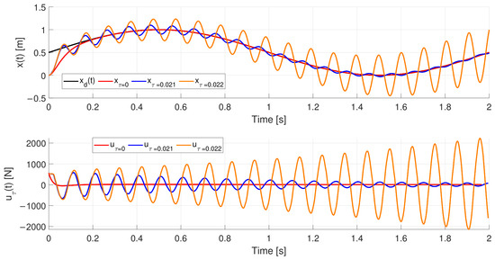
Simulations in this subsection were carried out using the $dde23$ numerical solver from MATLAB-2024a ©, considering $z(t-\tau )=[z_{1_0},0,0]$ for $t\in \{-\tau ,0\}$. As a nominal case, consider the linear single-delay system as defined in (10),with $a_0=20$ [N/mKg], $a_1=0.5$ [Ns/mKg] and $b_0=1$ [${\mathrm{Kg}}^{-1}$]. If no delay is considered, we can choose a desired stable second-order polynomial with $K_0={\omega }_n^2$ and $K_1=2\zeta {\omega }_n$ to ensure the asymptotic stability of the tracking error. By choosing ${\omega }_n=30$ and $\zeta =1$, with the aim of achieving fast convergence and critically damped behavior of the controller, it is possible to compute the critical time delay, using the classic 2D method [3], as ${\tau }^{\ast }=0.02162$ [s]. The desired trajectory to be followed by the system is set as $x_d=A+Bsin\left(2\pi ft\right)$, where $A=0.5$, $B=0.5$, and $f=0.5$. In this case, $z_{1_0}=0$. Figure 1 depicts simulation results for different time delays approaching and exceeding ${\tau }^{\ast }$.

Figure 1. Response of the linear force actuator system with delay (1) for several values of $\tau$ without considering $x_r$ in the controller (2).

If a delay is considered, we keep $K_0={\omega }_n^2$ and $K_1=2\zeta {\omega }_n$. In this case, we choose ${\delta }_0=1.005$ and $z_{1_0}=0$. On the one hand, using the 2D method, one can compute the critical delay as ${\tau }^{\ast }=0.11831$ [s]. On the other hand, considering Theorem 1 and using a standard numerical toolbox [41], the critical time delay is computed as ${\tau }^{\ast }=0.11667$ [s], which represents $98.61\%$ of the true critical time delay. Therefore, we obtain the following:

$$P=\left[\begin{array}{ccc}10.8262& 0.1062& -0.4106\\ 0.1062& 0.4526& -0.0503\\ -0.4106& -0.0503& 0.7487\end{array}\right]$$

$$Q=\left[\begin{array}{ccc}0.4084& -0.0456& -0.3224\\ -0.0456& 0.0063& 0.0449\\ -0.3224& 0.0449& 0.3643\end{array}\right]$$

$$R=\left[\begin{array}{ccc}1.2958& 0.1096& -0.0848\\ 0.1096& 0.0237& 0.0350\\ -0.0848& 0.0350& 0.2292\end{array}\right]$$

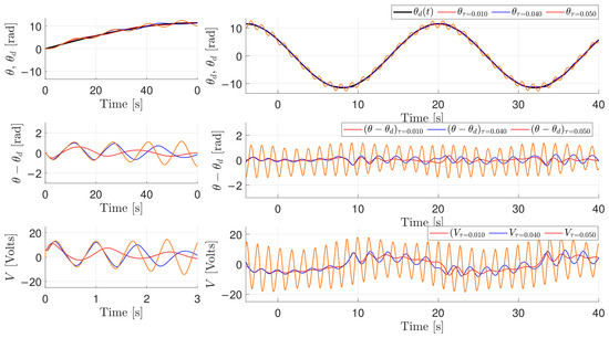
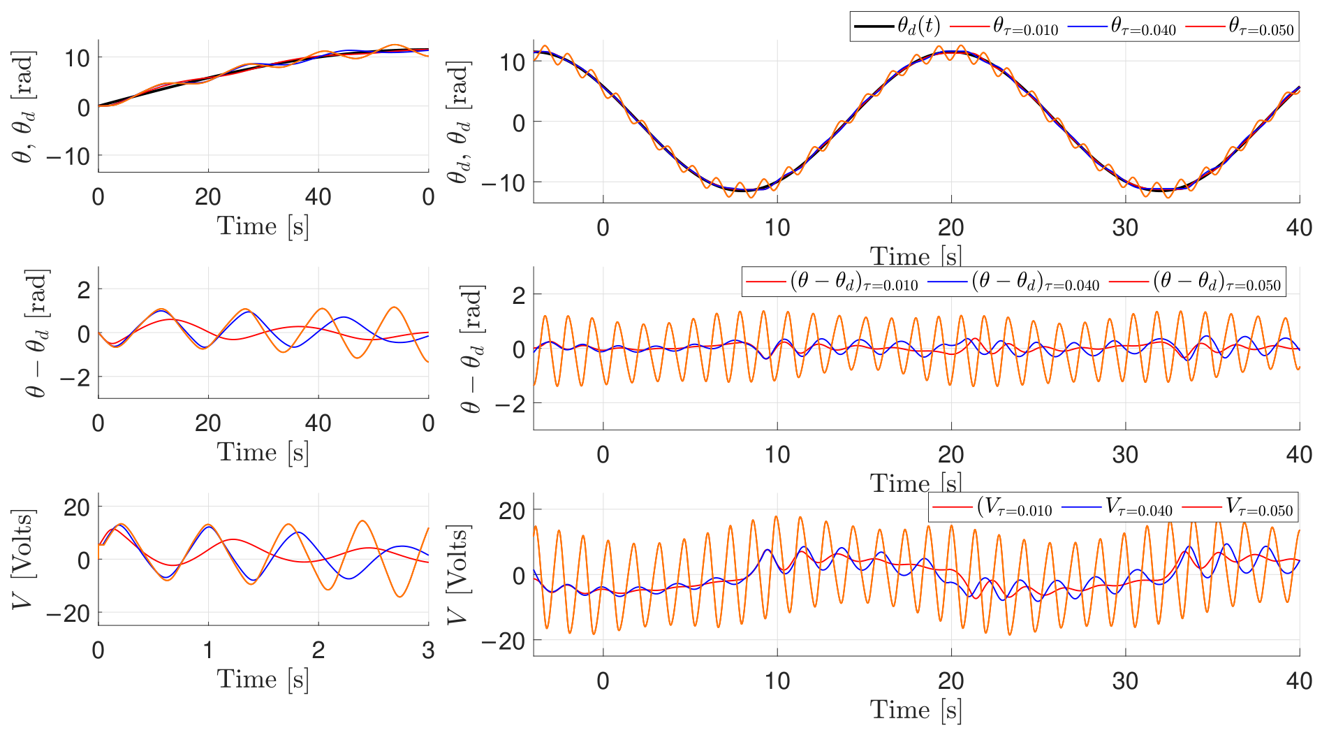
All matrices satisfy Theorem 1. Figure 2 depicts simulation results for different time delays approaching and exceeding ${\tau }^{\ast }$. Note that the desired trajectory $x_d\left(t\right)$ is represented in black and is tracked when the system is stable.

Figure 2. Response of delay linear force actuator system (1) for several values of $\tau$ considering the virtual reference trajectory $x_r$ in the controller (2).

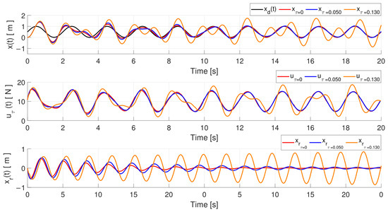
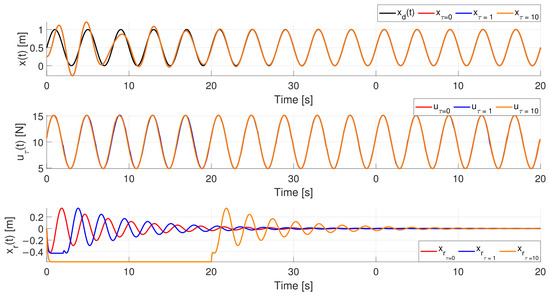
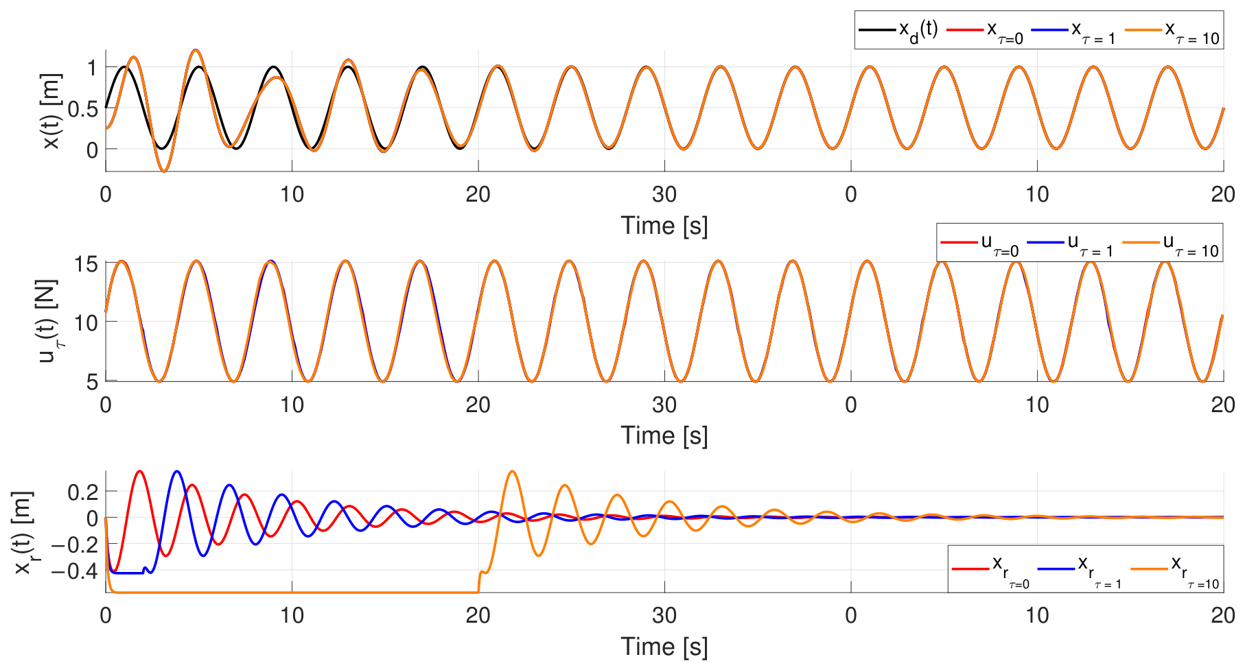
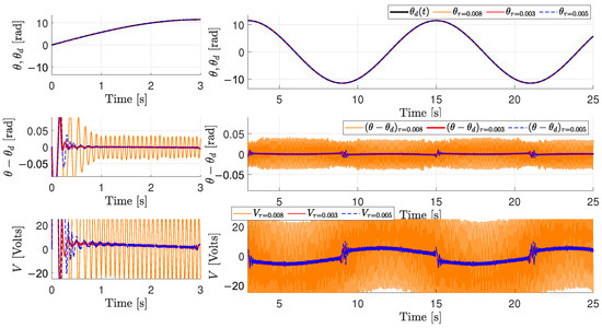
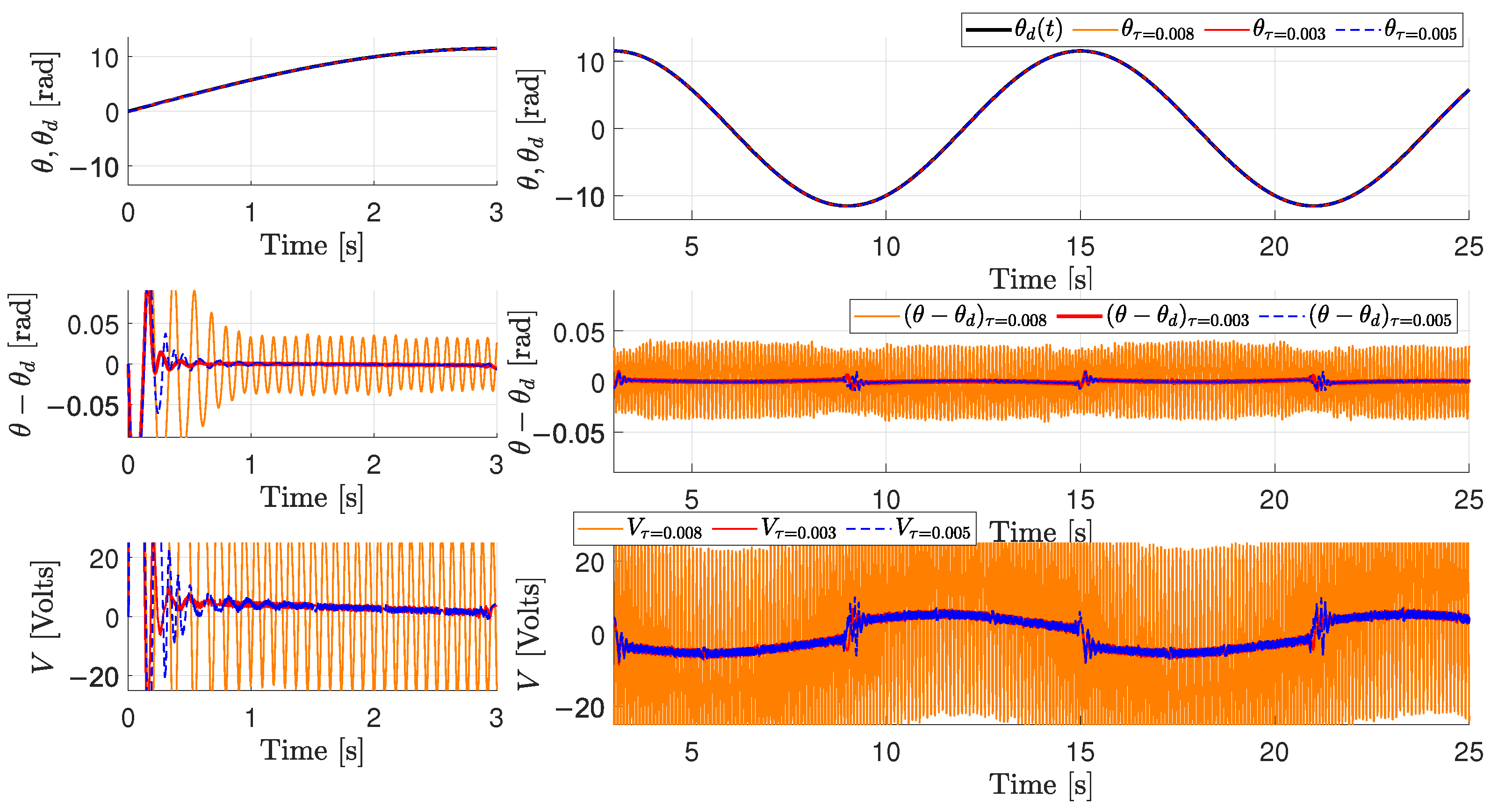
To further illustrate the case of stability independent of delay, we choose ${\delta }_0=1$ and set $z_{1_0}=0.25$, $K_0={\omega }_n^2$ and $K_1=2\zeta {\omega }_n$, with ${\omega }_n=30$ and $\zeta =1$. Figure 3 depicts simulation results for different time delays; note that the desired trajectory $x_d\left(t\right)$ is represented in black and is accurately tracked in all cases. The corresponding dynamics of the reference trajectory, which stabilize the control system, are also shown in Figure 3.

Figure 3. Response of the linear force actuator system with delay (1) depicting stability independent of delay.

4. Results on a DC Motor

In this section, we present simulation and experimental results to validate our proposal on a DC motor. First, the experimental testbed modeling and instrumentation are described. Then, comparative simulation results with the classic Smith predictor are presented. Finally, experimental results validate our proposal.

4.1. Testbed

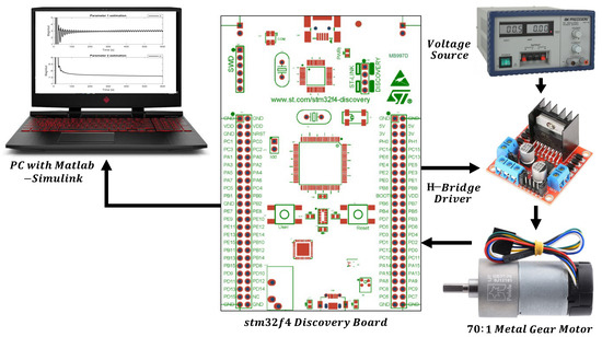
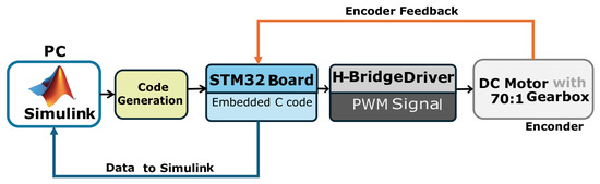
An experimental testbed based on a DC motor drive was developed to validate the proposed control strategy. The selected actuator was the DC motor, mainly for two reasons. First, many control technology implementations use DC motors as actuators. Second, there is extensive literature on their modeling and identification as linear dynamical systems [43]. The testbed consists of a brushed DC motor coupled to a 70:1 gear reduction stage. The motor shaft position $\theta$ is measured using an integrated Hall-effect sensor providing 16 pulses per revolution. By employing quadrature decoding, the encoder signal yields 64 counts per motor shaft revolution. Considering the gearbox reduction ratio, the resulting angular resolution at the output shaft corresponds to 3200 counts per revolution, allowing precise position measurement and velocity estimation. The DC motor actuation is achieved through an H-bridge driver controlled by an STM32f4 Discovery development board [44], which performs both control computation and signal generation. Pulse-width modulation (PWM) is used to regulate the motor voltage from 0–12 [V] with a switching frequency of 3.333 kHz. The control algorithms operate with a sampling period of 1 [ms]. Control algorithms are designed using a block-based approach in MATLAB/Simulink and automatically translated into C code, which is subsequently deployed onto the STM32-microcontroller for real-time execution. Also, it is important to mention that the time delay is artificially implemented by the transport-delay block from the MATLAB-Simulink library. This testbed setup enables real-time implementation and evaluation of control algorithms. Figure 4 depicts the component layout.

Figure 4. Testbed component layout.

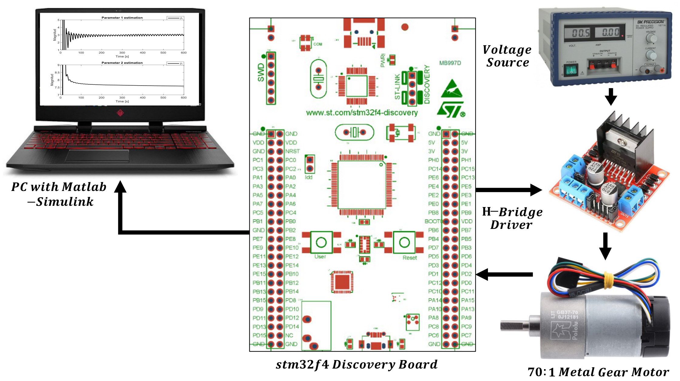
During experimental operation, the embedded controller executes the control routines independently while transmitting measured variables to a host computer running Simulink for monitoring, saving, and data visualization. This configuration enables direct comparison between theoretical and experimental responses while maintaining real-time execution constraints. The described platform provides a flexible environment for rapid prototyping and experimental validation of advanced control strategies applied to electromechanical systems. Figure 5 shows the operating schematic of the testbed.

Figure 5. Testbed operation diagram.

DC Motor Modeling and Identification

In this work, we consider the equation of the dynamical model of a geared DC motor with negligible inductance, linear friction, and without load, as given in Ref. [45], depicted in Equation (31).

$$J_m\ddot{\theta }+\left(f_m+{\displaystyle \frac{K_a{K}_b}{R_a}}\right)\dot{\theta }={\displaystyle \frac{K_a}{r{R}_a}}v$$

(31)

where $\dot{\theta }$ and $\ddot{\theta }$ represent the angular velocity and angular acceleration of the geared shaft, $J_m$ [Kg ${\mathrm{m}}^2$] represents the rotor inertia, $f_m$ [N m s] is the viscous friction coefficient, r [-] is the gear ratio, $K_a$ [Nm/A] is the motor-torque constant, $K_b$ [Vs] represents the back electromotive force constant, $R_a$ [$\Omega$] is the armature resistance and v [V] stands for the DC motor armature voltage. Considering the linear system described in (11), the corresponding model is obtained by dividing Equation (31) by $J_m$. Therefore, $a_2=1$ [-], $a_1=\left({\displaystyle \frac{f_m}{J_m}}+{\displaystyle \frac{K_a{K}_b}{J_m{R}_a}}\right)$ [${\mathrm{s}}^{-1}$], $a_0=0$ [${\mathrm{s}}^{-2}$] and $b_0={\displaystyle \frac{K_a}{r{J}_m{R}_a}}$ [(${\mathrm{V}}^{-1}$)]. Although the system under consideration is linear, several of its constant parameters remain unknown. Therefore, it is necessary to perform a parameter identification task to accurately determine the DC motor parameters. Provided that the model parameter $a_0=0$, and considering $y=\dot{\theta }$, then it can be reduced to a first-order linear dynamical system, normalized with respect to input parameter $b_0$; thus leading to Equation (32), where ${\widehat{P}}_1={\displaystyle \frac{1}{b_0}}$ [${\mathrm{Vs}}^2$] and ${\widehat{P}}_2={\displaystyle \frac{a_1}{b_0}}$ [Vs].

$${\widehat{P}}_1\dot{y}+{\widehat{P}}_{2}y=v$$

(32)

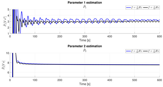
To obtain the linear model parameters, the algebraic identification approach was implemented; see [46] for details. The identification approach used a sinusoidal signal with different frequencies as input, as depicted in Figure 6. Therefore, the estimated values for the parameters are ${\widehat{P}}_1\approx 3$ [${\mathrm{Vs}}^2$] and ${\widehat{P}}_2\approx 7.6$ [Vs]. It is important to highlight that Equation (32) is used only for parameter identification purposes, while Equation (31) is used for control experimentation. Therefore, $a_2=1$, $a_1={\displaystyle \frac{7.6}{3}}$, $a_0=0$ and $b_0={\displaystyle \frac{1}{3}}$.

Figure 6. Convergence of the estimated values ${\widehat{P}}_1$ and ${\widehat{P}}_2$ for Equation (32).

4.2. Numerical Comparison of the Smith Predictor and the Virtual Reference Trajectory

Simulations in this subsection were carried out using MATLAB-Simulink ©, with the transport-delay block used to implement the delay in the corresponding feedback signals. In this case, the tracking error is defined as $e=\theta -{\theta }_d$. The controller gains were set as $K_0={\omega }_n^2$ and $K_1=2\zeta {\omega }_n$, with ${\omega }_n=35$, $\zeta =1$.

In [47], the author suggests that a time-delay compensator should be used when the process time delay is dominant; that is, when the normalized time delay ${\tau }_n={\displaystyle \frac{\tau }{\tau +T}}$ [-] is greater than 0.5, where $\tau$ is the time delay and T is the time constant of the system to be controlled. Considering the parameters obtained in the DC Motor Modeling and Identification section, it is straightforward to compute the time constant of the DC motor testbed as $T={\displaystyle \frac{2}{a_1}}\approx 0.78947$ [s].

To compare the performance of the proposed approach with that of the classical Smith predictor, a methodology similar to that presented in [48] was considered. Three cases for the comparative study using the normalized delay are defined as follows:

• Case 1: ${\displaystyle \frac{T}{\tau }}=5$, implying that ${\tau }_{C1}=0.1578$ [s] and ${\tau }_{n1}=0.1665$ [-].
• Case 2: ${\displaystyle \frac{T}{\tau }}=1$, implying that ${\tau }_{C2}=0.78947$ [s] and ${\tau }_{n2}=0.5000$ [-].
• Case 3: ${\displaystyle \frac{T}{\tau }}=0.5$, implying that ${\tau }_{C3}=1.578$ [s] and ${\tau }_{n3}=0.6665$ [-].

To quantitatively evaluate the results, we use the following metrics [49]:

$$\begin{array}{c}\hfill \begin{array}{ccc}\mathrm{ITSE}:={\int }_0^{t_f}t{(\theta -{\theta }_d)}^{2}dt,& & \mathrm{ITAE}:={\int }_0^{t_f}t\left|(\theta -{\theta }_d)\right|dt,\\ \mathrm{Max}\left(\mathrm{U}\right):=\underset{t}{max}\left\{\right|u_{\tau }\left|\right\},& & \mathrm{ICEC}:={\int }_0^{t_f}{\left(u_{\tau }\right)}^{2}dt\end{array}\end{array}$$

(33)

where ITSE is the integral of time-weighted square error, ITAE is the integral of time-weighted absolute error, Max(U) represents the maximum absolute value of the control signal, and ICEC is the integral of control energy consumption. Table 2 depicts the numerical results of a set of simulations for the three cases, both without noise and with noise at $10\%$ of the maximum amplitude of the desired trajectory. The delay considered for the SP is the nominal delay (${\tau }_{Ci}$ for $i=1,2,3$), while the VRT was designed, by computing ${\delta }_0$ with the 2D method, for a delay $50\%$ greater than the nominal delay for each case: ${\tau }_{VR{T}_{C1}}=0.2367$ [s] (${\delta }_0=1.0096$), ${\tau }_{VR{T}_{C2}}=1.1842$ [s] (${\delta }_0=1.002245$) and ${\tau }_{VR{T}_{C3}}=2.367$ [s] (${\delta }_0=1.0012$). The reason for this is that if the VRT controller were designed for the same delay as the SP controller, the VRT controller would be very close to instability.

Table 2. Performance comparison of the Smith predictor and the virtual reference trajectory.

Experimental Condition	Technique	Time Delay	ITSE	ITAE	Control Effort Max(U)	Control Energy Consumption ICEC
Without Noise	SP	${\tau }_{C1}$	44.2257	466.9742	722.4557	39,455.8
		${\tau }_{C2}$	1.1552	59.5450	722.4557	37,087.4
		${\tau }_{C3}$	3.9251	122.7284	722.4557	36,785.0
	VRT	${\tau }_{VR{T}_{C1}}$	0.0631	1.3332	20.4547	17,842.5
		${\tau }_{VR{T}_{C2}}$	1.2739	10.7153	23.1238	18,124.0
		${\tau }_{VR{T}_{C3}}$	1.2278	15.7533	20.0442	18,083.6
With 10 % Noise	SP	${\tau }_{C1}$	55.0328	441.6543	722.4557	458,573.1
		${\tau }_{C2}$	17.9564	256.0197	722.4557	384,134.8
		${\tau }_{C3}$	19.8510	265.0920	722.4557	400,221.9
	VRT	${\tau }_{VR{T}_{C1}}$	16.9797	251.4979	20.4477	17,766.2
		${\tau }_{VR{T}_{C2}}$	17.9950	254.6338	23.1784	18,129.0
		${\tau }_{VR{T}_{C3}}$	18.0202	255.6001	20.0422	18,085.5

Note: The simulation time was set to $t_f=100$ [s].

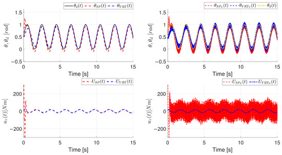
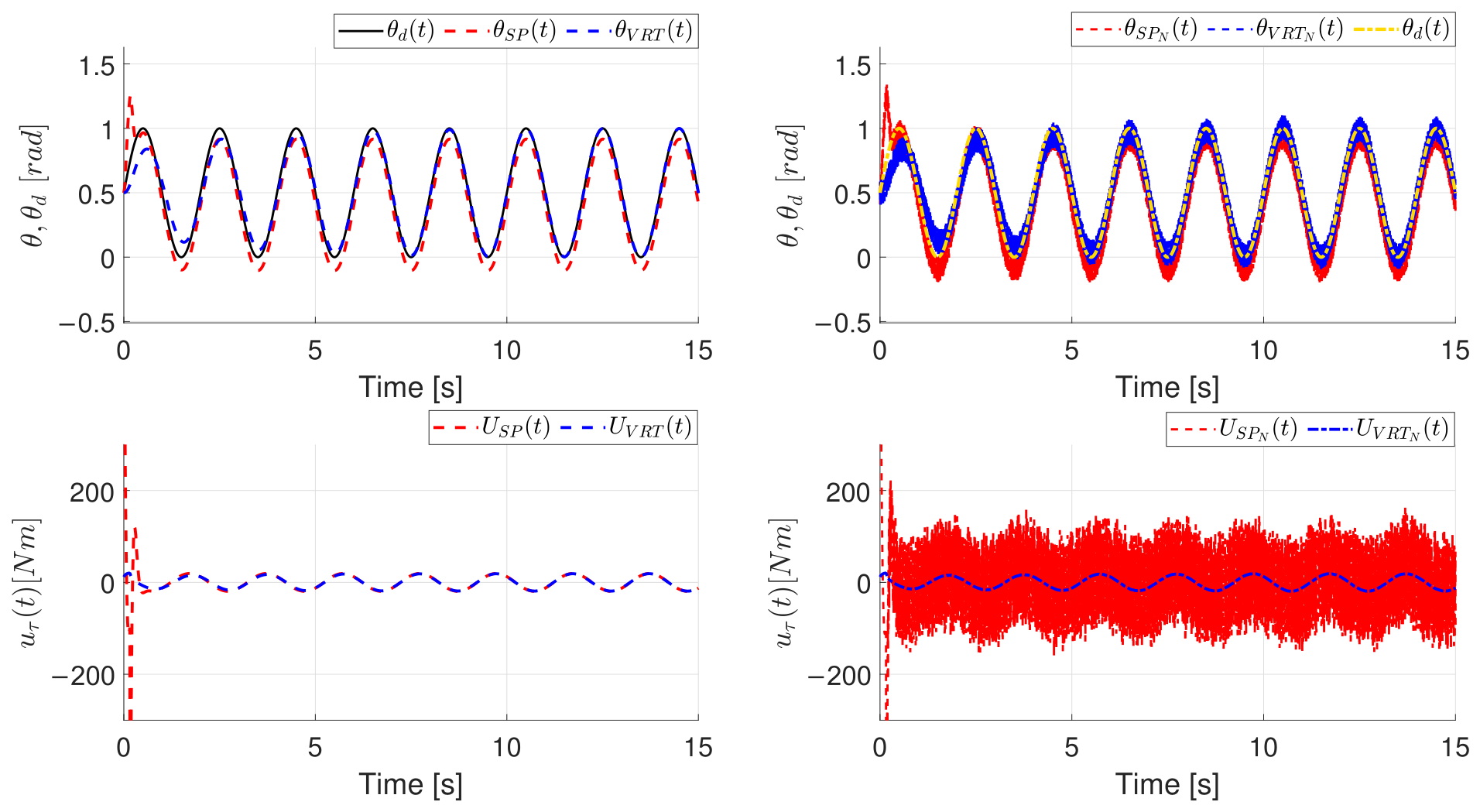
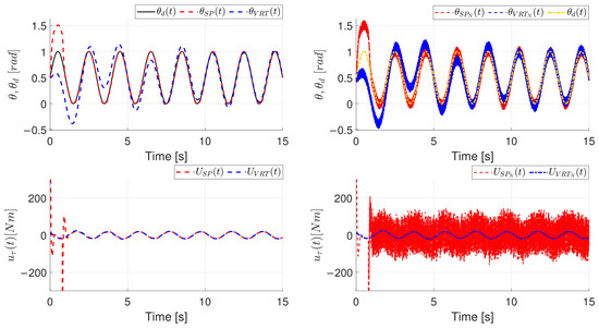
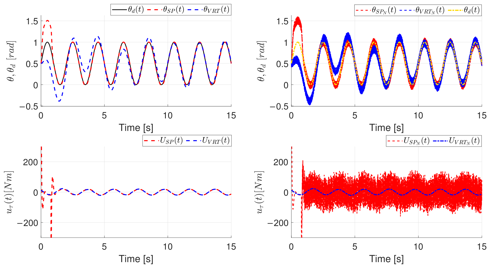
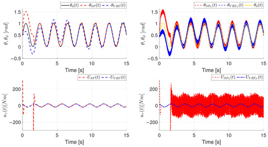
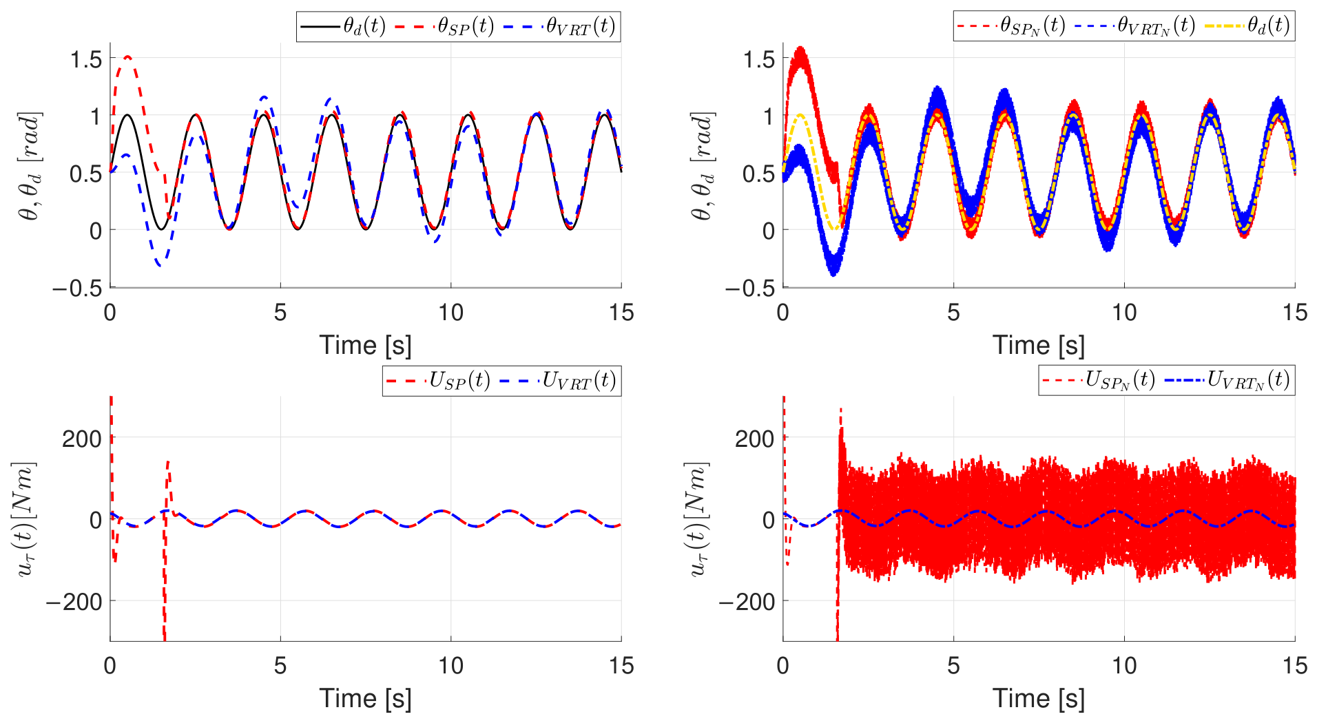
Figure 7, Figure 8 and Figure 9 graphically depict the simulation results for the comparative cases presented in Table 2. It is important to highlight that in the figures, only the first 15 [s] of the simulation are presented to better compare the transient behavior of the SP and VRT, while in Table 2, the results are presented for the large 100 [s] simulation. This better reflects the observation from the simulations presented in Figure 7, Figure 8 and Figure 9 that the VRT performance is worse than that of the SP if only a few seconds are considered for the metrics (33). On the one hand, considering the error metrics depicted in Table 2, for small time delays and without noise, the VRT outperforms the SP, with an ITSE more than 700 times lower and an ITAE 355 times lower. On the other hand, Table 1 clearly shows the superiority of the VRT regarding the control-oriented metrics: Max(U) indicates 36 times less control effort and ICEC indicates twice less energy than SP. When noise is considered, the Max(U) and ICEC metrics are almost the same, while the error metrics ITSE and ITAE deteriorate. Note that for Case 2, when the time delay matches the time constant of the DC motor (${\tau }_{n_2}=0.5$), both schemes show their most similar performance. In general, the VRT presents better metrics over the large, while during the transient, its performance is comparable with that of the SP.

Figure 7. Comparison of the SP and VRT approaches for Case 1, without noise (left) and with noise (right).

Figure 8. Comparison of the SP and VRT approaches for Case 2, without noise (left) and with noise (right).

Figure 9. Comparison of the SP and VRT approaches for Case 3, without noise (left) and with noise (right).

Experimental Results

In this section, experimental tests of the control of the DC motor testbed described in Section 4.1 with artificial time-delay measurement are depicted to experimentally validate our proposal. It is important to mention that the available measured signal is the motor angular position, while the angular velocity $\dot{\theta }$ is obtained via a Luenberger observer. The desired trajectory to be followed by the system is set as ${\theta }_d=A+Bcos\left(2\pi ft\right)$, where $A=0$ [rad], $B=11.5$ [rad], and $f={\displaystyle \frac{1}{12}}$ [Hz], starting from the rest position.

Figure 10 shows the response of the DC motor without considering the reference trajectory ${\theta }_r$ with $K_0={\omega }_n^2$ and $K_1=2\zeta {\omega }_n$, with ${\omega }_n=100$, $\zeta =1$. In this case, the maximum delay can be computed as ${\tau }^{\ast }=0.00653$ [s]. Clearly, with $\tau =0.0030$ [s] and $\tau =0.0050$ [s], the system is stable and the tracking error $\theta -{\theta }_d$ is practically zero. When $\tau =0.0080$ [s], the system becomes unstable even as the trajectory tracking is good, as one can conclude from the saturated control signal V and the increased tracking error.

Figure 10. Experimental results for the DC motor controlled with the proposed controller without considering the virtual trajectory ${\theta }_r$.

Figure 11 shows the response of the DC motor considering the reference trajectory ${\theta }_r$ with $K_0={\omega }_n^2$ and $K_1=2\zeta {\omega }_n$, with ${\omega }_n=100$, $\zeta =1$, and ${\delta }_0=1.01$. In this case, the maximum delay can be computed as ${\tau }^{\ast }=0.02604$ [s]. Clearly, with $\tau =0.010$ [s] and $\tau =0.040$ [s], the system is stable and the tracking error $\theta -{\theta }_d$ is practically zero. When $\tau =0.050$ [s], the system becomes unstable, as one can conclude from the control signal V and the increased tracking error. It is observed that the critical delay ${\tau }^{\ast }$ is lower than the experimentally observed stability bound of $\tau =0.040$ [s], but unstable for $\tau =0.050$ [s]. To explain this experimental fact, it is important to mention that the experiments showed that the use of the PWM signal provides the proposed approach with some additional stability robustness [50]. Nonetheless, its theoretical analysis lies beyond the scope of this work. Additionally, it is important to mention that for larger values of $\tau$, the demand for control effort is greater; thus, experimentally, we are limited to compensating for certain values of delay, as depicted in the experiments in this section.

Figure 11. Experimental results for the DC motor controlled with the proposed controller and the virtual reference trajectory ${\theta }_r$.

5. Conclusions

In this work, a novel proposal for the control of linear actuator systems with a single time delay is introduced. The paradigm shift lies in the addition of a virtual reference trajectory generator to the desired trajectory, which reconstructs delayed tracking information directly from measured delayed errors. As shown, the introduction of such virtual reference dynamics into the system model yields a standard neutral time-delay system, whose stability can be rigorously analyzed using state-of-the-art Lyapunov–Krasovskii-based methods, particularly by solving LMIs and BMIs. As a major advantage, the proposed approach eliminates the need for explicit knowledge or prediction of the delay, rendering stability independent of the time delay in the ideal case or enlarging the admissible delay margin while preserving the original controller architecture, thus reducing implementation complexity. The presented results show the effectiveness of our proposal. Simulation results allow us to conclude that, without noise, the VRT scheme presents up to 700 times lower ITSE metrics, 36 times less Max(U) metrics, and half the control energy consumption, ICEC, for small delays, while for time delays matching the time constant of the system, its performance is comparable with that of the SP. Interestingly, when the time delay matches the actuator time constant, both schemes achieve similar performance. The experimental validation was successful, though challenging due to hardware constraints. Future research directions include extensions to systems with multiple delays, where the interaction between delays might introduce more complexity; the application to nonlinear control systems, a broader class of dynamical systems; and the inclusion of bounded control inputs in the theoretical analysis, bridging the gap between theory and practical actuator limits.

References

- Lamnabhi-Lagarrigue, F.; Annaswamy, A.; Engell, S.; Isaksson, A.; Khargonekar, P.; Murray, R.M.; Nijmeijer, H.; Samad, T.; Tilbury, D.; Van den Hof, P. Systems and Control for the future of humanity, research agenda: Current and future roles, impact and grand challenges. Annu. Rev. Control 2017, 43, 1–64. [Google Scholar] [CrossRef] [Scilit]
- Fridmann, E. Introduction to Time-Delay Systems; Birkhäuser: Cham, Switzerland, 1981. [Google Scholar]
- Gu, K.; Vladimir L. Kharitonov, J.C. Stability of Time-Delay Systems; Birkhäuser: Boston, MA, USA, 2003. [Google Scholar]
- Milton, J.G. Time delays and the control of biological systems: An overview. IFAC-PapersOnLine 2015, 48, 87–92. [Google Scholar] [CrossRef] [Scilit]
- Park, J.H.; Lee, T.H.; Liu, Y.; Chen, J. Dynamic Systems with Time Delays: Stability and Control; Springer: Berlin/Heidelberg, Germany, 2019; Volume 4. [Google Scholar]
- Zhang, X.M.; Han, Q.L. Time-delay systems and their applications. Int. J. Syst. Sci. 2022, 53, 2477–2479. [Google Scholar] [CrossRef] [Scilit]
- Zhou, B.; Liu, Q.; Mazenc, F. Stabilization of linear systems with both input and state delays by observer–predictors. Automatica 2017, 83, 368–377. [Google Scholar] [CrossRef] [Scilit]
- Deng, Y.; Léchappé, V.; Moulay, E.; Zhang Chen, B.L.; Plestan, F.; Han, Q.L. Predictor-based control of time-delay systems: A survey. Int. J. Syst. Sci. 2022, 53, 2496–2534. [Google Scholar] [CrossRef] [Scilit]
- Báez-Hernández, J.A.; Velasco-Villa, M.; Mondié, S. Non-Linear Prediction-Based Trajectory Tracking for Non-Holonomic Mobile Robots. IEEE Access 2023, 11, 124265–124277. [Google Scholar] [CrossRef] [Scilit]
- Nguyen, C.M.; Zemouche, A.; Trinh, H. Observer-based control design for nonlinear systems with unknown delays. IEEE Trans. Circuits Syst. II Express Briefs 2021, 69, 1327–1331. [Google Scholar] [CrossRef] [Scilit]
- Li, W.; Zhang, Z.; Ge, S.S. Observer-based output-feedback control for nonlinear time-delay systems. IEEE Trans. Syst. Man. Cybern. Syst. 2022, 53, 3514–3526. [Google Scholar]
- Luviano-Juárez, A.; Ramírez-Neria, M.; González-Sierra, J. Robust Trajectory Tracking for Omnidirectional Mobile Robots with Input Time Delay: An ADRC Approach. Mathematics 2026, 14, 266. [Google Scholar] [CrossRef] [Scilit]
- Kawano, Y.; Ahmed, S.; Cucuzzella, M.; Scherpen, J.M. Passivity of nonlinear time-delay systems. IFAC-PapersOnLine 2023, 56, 8568–8573. [Google Scholar] [CrossRef] [Scilit]
- Gómez-Rosas, C.; Portillo-Veléz, R.J. Time delay compensation in a bilateral teleoperation system. In Proceedings of the 2021 XXIII Robotics Mexican Congress (ComRob), Tijuana, Mexico, 27–29 October 2021; pp. 13–18. [Google Scholar] [CrossRef] [Scilit]
- Polushin, I.G. A Generalized Scattering Framework for Teleoperation with Communication Delays. IFAC-PapersOnLine 2020, 53, 10064–10069. [Google Scholar] [CrossRef] [Scilit]
- Ma, Y.-h.; Zhang, S.; He, X.-y.; Liu, Z.-j. A survey of delay compensation and control based on continuum backstepping control algorithms for time-delay systems. Chin. J. Eng. 2022, 44, 1053–1061. [Google Scholar]
- Vazquez, R.; Auriol, J.; Bribiesca-Argomedo, F.; Krstic, M. Backstepping for partial differential equations: A survey. Automatica 2026, 183, 112572. [Google Scholar] [CrossRef] [Scilit]
- Ji, X.A.; Orosz, G. Learn from one and predict all: Single trajectory learning for time delay systems. Nonlinear Dyn. 2024, 112, 3505–3518. [Google Scholar] [CrossRef] [Scilit]
- Neto, A.A. Reinforcement Learning for Control Systems with Time Delays: A Comprehensive Survey. arXiv 2026, arXiv:2602.00399. [Google Scholar]
- Krasovskii, N.N. The Stability of Motion; Stanford University Press: Stanford, CA, USA, 1963. [Google Scholar]
- Chaillet, A.; Karafyllis, I.; Pepe, P.; Wang, Y. The ISS framework for time-delay systems: A survey. Math. Control. Signals Syst. 2023, 35, 237–306. [Google Scholar] [CrossRef] [Scilit]
- Zhang, H.; Xia, J.; Zhuang, G. Improved delay-dependent stability analysis for linear time-delay systems: Based on homogeneous polynomial Lyapunov–Krasovskii functional method. Neurocomputing 2016, 193, 176–180. [Google Scholar] [CrossRef] [Scilit]
- Sun, J.; Chen, J. A survey on Lyapunov-based methods for stability of linear time-delay systems. Front. Comput. Sci. 2017, 11, 555–567. [Google Scholar]
- de Oliveira, F.S.S.; Souza, F.O. Improved delay-dependent stability criteria for linear systems with multiple time-varying delays. Int. J. Control 2021, 94, 3415–3423. [Google Scholar] [CrossRef] [Scilit]
- Ren, Y.; Li, Q.; Liu, K.-Z.; Ding, D.-W. A successive convex optimization method for bilinear matrix inequality problems and its application to static output-feedback control. Int. J. Robust Nonlinear Control 2021, 31, 9709–9730. [Google Scholar] [CrossRef] [Scilit]
- Mushtaq, T.; Seiler, P.; Hemati, M.S. On the convexity of static output feedback control synthesis for systems with lossless nonlinearities. Automatica 2024, 159, 111380. [Google Scholar] [CrossRef] [Scilit]
- Mahmoud, M.S. Chapter One—An overview of time-delay control systems. In Control Strategy for Time-Delay Systems; Khooban, M.H., Dragicevic, T., Eds.; Emerging Methodologies and Applications in Modelling, Identification and Control; Academic Press: New York, NY, USA, 2021; pp. 1–82. [Google Scholar] [CrossRef] [Scilit]
- Barkas, D.A.; Ioannidis, G.C.; Psomopoulos, C.S.; Kaminaris, S.D.; Vokas, G.A. Brushed DC motor drives for industrial and automobile applications with emis on control techniques: A comprehensive review. Electronics 2020, 9, 887. [Google Scholar] [CrossRef] [Scilit]
- Al-Tamimi, A.; Al-Momani, F.; Salah, M.; Banihani, S.; Al-Jarrah, A. Control Strategies for DC Motor Systems Driving Nonlinear Loads in Mechatronic Applications. Actuators 2026, 15, 175. [Google Scholar] [CrossRef] [Scilit]
- Léchappé, V.; Rouquet, S.; Gonzalez, A.; Plestan, F.; De Leon, J.; Moulay, E.; Glumineau, A. Delay estimation and predictive control of uncertain systems with input delay: Application to a DC motor. IEEE Trans. Ind. Electron. 2016, 63, 5849–5857. [Google Scholar] [CrossRef] [Scilit]
- Tahtawi, A.; Baisrum, B.; Jadmiko, S. Speed control of DC motor based on wireless networked control system with time delay and saturation parameters. In IOP Conference Series: Materials Science and Engineering; IOP Publishing: Bristol, UK, 2020; Volume 830, p. 032025. [Google Scholar]
- Dharshan, Y.; Sharmila, B.; Kaushik, S.; Kavimalar, K. Certain investigation of real time networked control dc motor using smith predictor. Turk. J. Comput. Math. Educ. 2021, 12, 180–187. [Google Scholar] [CrossRef] [Scilit]
- Maleki, N.; Moradi, E. Robust H∞ Control of DC Motor in the Presence of Input Delay and Disturbance by the Predictor-Based Method. Complexity 2022, 2022, 1902166. [Google Scholar] [CrossRef] [Scilit]
- Chen, J.X.; Fan, G.X.; Li, X.G.; Mao, Z.Z. Stability analysis for dc motor drive systems with time delays. In Proceedings of the 2022 34th Chinese Control and Decision Conference (CCDC), Hefei, China, 15–17 August 2022; pp. 2942–2947. [Google Scholar]
- Kuzu, İ.; Ayasun, S. Computation of Robust Stability Delay Margin for Time-Delay DC Motor Speed Control System. In Proceedings of the 2024 15th National Conference on Electrical and Electronics Engineering (ELECO), Bursa, Turkiye, 28–30 November 2024; pp. 1–5. [Google Scholar]
- Subramanian, M. Tradeoff Techniques for Stabilization of Network-Controlled DC Motor Speed Control System with Uncertainties. Electr. Power Compon. Syst. 2023, 52, 2828–2845. [Google Scholar] [CrossRef] [Scilit]
- Portillo-Vélez, R.D.; Rodriguez-Angeles, A.; Cruz-Villar, C.A. An optimization-based impedance approach for robot force regulation with prescribed force limits. Math. Probl. Eng. 2015, 2015, 918301. [Google Scholar] [CrossRef] [Scilit]
- Caballero-Mora, J.A.; de Jesús Portillo-Vélez, R.; Vásquez-Santacruz, J.A.; López-González, A.; Hernández-Martínez, E.G. Admittance-based robot force control without velocity and force sensors. Control Theory Technol. 2025, 23, 494–512. [Google Scholar] [CrossRef] [Scilit]
- Chen, C.T. Linear System Theory and Design; Oxford University Press: Oxford, UK, 2012; p. 352. [Google Scholar]
- Kharitonov, V.; Plischke, E. Lyapunov matrices for time-delay systems. Syst. Control Lett. 2006, 55, 697–706. [Google Scholar] [CrossRef] [Scilit]
- VanAntwerp, J.G.; Braatz, R.D. A tutorial on linear and bilinear matrix inequalities. J. Process Control 2000, 10, 363–385. [Google Scholar] [CrossRef] [Scilit]
- Vimalesh, A.; An, J.; Ahn, J.H.; Kim, H.Y. System modeling and identification of a balance type checkweigher compensated by voice coil actuator. Adv. Mech. Eng. 2019, 11, 1687814019884425. [Google Scholar] [CrossRef] [Scilit]
- Kuczmann, M. Review of DC motor modeling and linear control: Theory with laboratory tests. Electronics 2024, 13, 2225. [Google Scholar] [CrossRef] [Scilit]
- STMicroelectronics. STM32F4DISCOVERY. 2025. Available online: https://www.st.com/en/evaluation-tools/stm32f4discovery.html (accessed on 8 July 2026).
- Kelly, R.; Santibáñez, V. Control de Movimiento de Robots Manipuladores; Pearson Educación: Madrid, Spain, 2003. [Google Scholar]
- Sira-Ramírez, H.; Rodríguez, C.G.; Cortés Romero, J.; Juárez, A.L. Algebraic Identification and Estimation Methods in Feedback Control Systems; John Wiley & Sons: New York, NY, USA, 2014. [Google Scholar]
- Normey-Rico, J.E.; Camacho, E.F. Dead-time compensators: A survey. Control Eng. Pract. 2008, 16, 407–428. [Google Scholar] [CrossRef] [Scilit]
- Ingimundarson, A.; Hägglund, T. Performance comparison between PID and dead-time compensating controllers. J. Process Control 2002, 12, 887–895. [Google Scholar] [CrossRef] [Scilit]
- Gómez, D.; Moya, E.J.; Baeyens, E. Control performance assessment: A general survey. In Distributed Computing and Artificial Intelligence: 7th International Symposium; Springer: Berlin/Heidelberg, Germany, 2010; pp. 621–628. [Google Scholar]
- Hou, L.; Michel, A.N. Stability analysis of pulse-width-modulated feedback systems. Automatica 2001, 37, 1335–1349. [Google Scholar] [CrossRef] [Scilit]
Disclaimer/Publisher’s Note: The statements, opinions and data contained in all publications are solely those of the individual author(s) and contributor(s) and not of MDPI and/or the editor(s). MDPI and/or the editor(s) disclaim responsibility for any injury to people or property resulting from any ideas, methods, instructions or products referred to in the content. |
© 2026 by the authors. Licensee MDPI, Basel, Switzerland. This article is an open access article distributed under the terms and conditions of the Creative Commons Attribution (CC BY) license.