A Difference Equation Matrix Model Predictive Control Approach Applied to a Distillation Column

Abstract

The Difference Equation Matrix Model (DEMM) is presented as an input–output Model Predictive Control (MPC) formulation derived from discrete difference equations. The proposed approach is compared with the widely used Dynamic Matrix Control (DMC) strategy from a structural perspective, highlighting differences in model parameterization, identification requirements, and matrix dimensions. The analysis indicates that DEMM provides a more compact model representation than the DMC formulation considered in this work while preserving the predictive-control framework. Furthermore, the DEMM strategy is applied to a binary distillation column, a multivariable nonlinear process, to illustrate its implementation and closed-loop behavior under disturbance, noise, and setpoint-change scenarios. Simulation results demonstrate satisfactory disturbance-rejection and tracking performance for the considered operating conditions.

1. Introduction

Industrial systems have long presented significant challenges to control engineering, with increasingly demanding processes exhibiting complex behaviors such as nonlinearities and time delays that overwhelm traditional control strategies. One of the most widely adopted advanced control strategies used to address these challenges is Model Predictive Control (MPC). In MPC, the system to be controlled is represented by a mathematical model that is used both to determine the control action and to predict the future response of the system, enabling prediction of future plant behavior and online optimization of the control action. MPC strategies have proven to be highly effective multivariable controllers, capable of handling processes with strong interactions and explicit constraints [1].

Thanks to these capabilities, MPC has found widespread application across multiple fields, ranging from industrial environments such as Heating, Ventilation, and Air Conditioning (HVAC) systems [2] to specialized equipment in the aerospace domain [3].

A comprehensive review of MPC-based Sliding Mode Controllers (SMCs) was presented in [4], demonstrating their effectiveness in applications including process systems, electromechanical systems, and energy systems. Two main approaches were identified: one in which MPC is employed during the reaching phase to ensure that the system attains sliding mode, and another in which MPC governs the system once the sliding phase has been achieved. The authors also identified several open challenges, such as the requirement for full-state measurement, the need for accurate system models, and the well-known issue of chattering in sliding controllers. Furthermore, they highlighted promising research directions, including applications to large-scale distributed systems, the use of SMCs in financial market modeling, and the development of event-triggered algorithms to reduce computational costs.

The problem of obtaining accurate models and updating them dynamically remains an active research topic in MPC. A widely adopted solution involves the use of Neural Networks, as demonstrated in [5], where a deep learning-based MPC framework is implemented for quadcopter flight control. The main contribution of that work lies in optimizing the framework to minimize computation time, thereby preserving modeling accuracy while enabling real-time operation. Similarly, in [6], a neural network model is shown to substantially reduce the number of calculations per control action compared to conventional two-step MPC for the control of permanent magnet synchronous motors.

Another example highlighting the relevance of MPC is presented in [7], which proposes an enhanced MPC strategy for motor torque control. The study compares traditional Direct Torque Control with Model Predictive Direct Torque Control and the proposed enhanced MPC approach. The improved implementation demonstrates reduced torque and flux ripples—common drawbacks of Direct Torque Control—without increasing computational complexity.

Within the MPC family, there are multiple formulations or derived families, for example Generalized Predictive Control (GPC) [8] or Dynamic Matrix Control (DMC); the latter has become one of the most widely used advanced process-control strategies in industry [9]. DMC was originally introduced by Cutler and Ramaker [10] and is based on the step response of the system. It has proven particularly effective for Multiple-Input Multiple-Output (MIMO) systems due to its ability to handle multivariable interactions and process constraints.

Although DEMM shares the predictive-control philosophy of Generalized Predictive Control (GPC), the two approaches differ in the way future predictions are obtained. Classical GPC formulations are commonly derived from CARIMA-type polynomial models and rely on Diophantine equations to construct the prediction matrices. In contrast, DEMM generates the predictive model directly from identified difference equations, leading to an explicit matrix formulation based on the estimated input–output dynamics. The objective of the present work is not to establish a detailed comparison with GPC, but rather to introduce the DEMM formulation and compare its model structure with the widely adopted DMC framework.

An illustrative example of DMC implementation is provided in [11], where a PID-based DMC controller is applied to an engraving machine system. The proposed approach improves control speed and reduces overshoot. However, the authors report that tuning the PID parameters remains a significant challenge, while computational demand is not explicitly discussed despite the controller’s strong performance.

In [12], DMC is employed for State of Charge (SOC) estimation in a battery pack, an application where MPC-based techniques are widely used due to their precision. Such models must be continuously updated to account for deviations from real system behavior caused by changes in operating conditions. To address this issue, the proposed approach combines DMC with an Extended Kalman Filter (EKF) that processes voltage and current measurements, enabling real-time model recalibration and sustained estimation accuracy.

As in any active research field, new controller variants are continuously proposed. For instance, ref. [13] introduces a generalized DMC for open-loop unstable processes, achieving effective disturbance rejection in systems with integrating or unstable dynamics. Likewise, ref. [14] presents an improved DMC formulation incorporating output penalties to reduce overshoot in complex systems without increasing computational complexity.

Chemical processes often exhibit strong nonlinearities and delays arising from reaction dynamics or equipment characteristics. MPC has been widely adopted in such applications due to the availability of process models and its predictive capabilities. A prominent example is distillation columns, which require the simultaneous monitoring and control of multiple variables, such as component concentrations and temperatures [15].

An example of this application is presented in [16], where a coal-to-ethylene glycol distillation unit is modeled using a closed-loop subspace identification approach to design a DMC controller. The resulting system demonstrates robustness and strong disturbance rejection. A similar application is reported in [17] for benzene–toluene distillation.

In [18], the limitations of PID control for distillation processes are discussed, and DMC is shown to outperform both PID and fuzzy controllers. In contrast, the present work does not employ fuzzy logic as a competing controller, but rather as a modeling tool to support and enhance MPC performance.

In [19], a Butylene–Butane Distillation Column (BBDC) is controlled using a High-Order Iterative Learning Control (HOILC) strategy. The multicomponent distillation process is simplified to a binary model, to which the iterative learning algorithm is applied.

A Heat-Integrated Distillation Column (HIDiC) is introduced in [20] as an energy-efficient distillation configuration. The authors employ a nonlinear mechanistic model of the HIDiC to tune a Proportional–Integral (PI) controller using a Genetic Algorithm. Simulation results show promising setpoint tracking and disturbance rejection performance; however, the authors note that real-world implementation may face challenges related to computational cost, scalability, and convergence.

Finally, ref. [21] presents a control analysis of a Side-Stream Extractive Distillation (SSED) column, a configuration known for high energy consumption. To mitigate this issue, the authors propose an improved design that achieves enhanced economic performance through optimization and sensitivity analysis.

It should be noted that DEMM belongs to the broader family of input–output model predictive control approaches. Similar to transfer-function, ARX-based, and Generalized Predictive Control formulations, it employs a discrete-time input–output representation of the plant. The contribution of this work is not the introduction of a new predictive-control paradigm, but rather the development of a compact matrix formulation derived directly from difference equations and its application to the control of a nonlinear distillation process.

The remainder of this paper is organized as follows. Section 2 describes the DEMM algorithm. Section 3 presents a comparison between DEMM and DMC. Section 4 details the distillation column considered in this study. Finally, Section 5 presents the conclusions of the study.

2. Difference Equation Matrix Model

As its name implies, the Difference Equation Matrix Model (DEMM) algorithm utilizes a difference equation to generate the model of the plant. This is a basic approach for discrete control strategies, where a linear model of the system is represented by an equation that relates a certain number of past inputs to the system and their corresponding outputs. This past information constitutes the state variables of the system and results in a SISO model as follows:

$${\mathsf{y}}_{\mathsf{p}}={\alpha }_{\mathsf{0}}+\left({\alpha }_{\mathsf{1}}·{\mathsf{x}}_{\mathsf{p}-\mathsf{1}}+\dots +{\alpha }_{\mathsf{m}}·{\mathsf{x}}_{\mathsf{p}-\mathsf{m}}\right)-\left({\beta }_{\mathsf{1}}·{\mathsf{y}}_{\mathsf{p}-\mathsf{1}}+\dots +{\beta }_{\mathsf{m}}·{\mathsf{y}}_{\mathsf{p}-\mathsf{m}}\right)$$

(1)

where $\left({\mathsf{x}}_{\mathsf{i}},{\mathsf{y}}_{\mathsf{i}}\right)$ denote the input–output pair of the plant at sample $\mathsf{i}$, with ${\mathsf{x}}_{\mathsf{i}}$ representing the control input and ${\mathsf{y}}_{\mathsf{i}}$ the measured output. This means that a present output ${\mathsf{y}}_{\mathsf{p}}$ can be obtained as a consequence of the past inputs and outputs $\{\left({\mathsf{y}}_{\mathsf{p}-\mathsf{1}},{\mathsf{x}}_{\mathsf{p}-\mathsf{1}}\right),\left({\mathsf{y}}_{\mathsf{p}-\mathsf{2}},{\mathsf{x}}_{\mathsf{p}-\mathsf{2}}\right),\cdots ,$$\left({\mathsf{y}}_{\mathsf{p}-\mathsf{m}},{\mathsf{x}}_{\mathsf{p}-\mathsf{m}}\right)\}$, going as far back as $\mathsf{m}$ samples (the dynamic memory of the system). The coefficients ${\alpha }_{\mathsf{i}}$ and ${\beta }_{\mathsf{i}}$ are the model parameters that must be adjusted for the equation to represent the behavior of a specific plant (the method to obtain them will be discussed later in the article), with ${\alpha }_{\mathsf{0}}$ representing the initial default value of the system (at the start of the experiment, with all past values equal to zero).

For simplicity of presentation, Equation (1) is written using the same maximum lag order for both input and output variables. However, the DEMM formulation is not restricted to this assumption. In practical applications, different input and output lag orders, as well as explicit input delays, can be accommodated by including the corresponding terms in the model structure. The distillation-column example presented in Section 4 illustrates this situation, where different input delays appear in the identified model.

Equation (1) can be reformulated into an incremental function, dependent on changes in the input signals:

$${\mathsf{y}}_{\mathsf{p}}=\left({\alpha }_{\mathsf{1}}·\mathsf{\Delta }{\mathsf{x}}_{\mathsf{p}-\mathsf{1}}+\cdots +{\alpha }_{\mathsf{m}}·\mathsf{\Delta }{\mathsf{x}}_{\mathsf{p}-\mathsf{m}}\right)-\left({\widehat{\beta }}_{\mathsf{1}}·{\mathsf{y}}_{\mathsf{p}-\mathsf{1}}+\cdots +{\widehat{\beta }}_{\mathsf{m}}·{\mathsf{y}}_{\mathsf{p}-\mathsf{m}}+{\widehat{\beta }}_{\mathsf{m}+\mathsf{1}}·{\mathsf{y}}_{\mathsf{p}-\mathsf{m}-\mathsf{1}}\right)$$

(2)

where $\mathsf{\Delta }{\mathsf{x}}_{\mathsf{i}}={\mathsf{x}}_{\mathsf{i}}-{\mathsf{x}}_{\mathsf{i}-\mathsf{1}}$ and the new ${\widehat{\beta }}_{\mathsf{i}}$ parameters are obtained from the differences of the previous ones: $\left\{{\widehat{\beta }}_{\mathsf{1}}={\beta }_{\mathsf{1}}-1,{\widehat{\beta }}_{\mathsf{2}}={\beta }_{\mathsf{2}}-{\beta }_{\mathsf{1}},\cdots ,{\widehat{\beta }}_{\mathsf{m}}={\beta }_{\mathsf{m}}-{\beta }_{\mathsf{m}-\mathsf{1}},{\widehat{\beta }}_{\mathsf{m}+\mathsf{1}}=-{\beta }_{\mathsf{m}}\right\}$.

This modeling approach can be further extended by including future inputs and outputs, that is, by defining a prediction horizon $\mathsf{h}$. The result is the following matrix equation:

$$\left[\begin{array}{ccccccc}1& {\widehat{\beta }}_{\mathsf{1}}& \cdots & {\widehat{\beta }}_{\mathsf{m}+\mathsf{1}}& 0& \cdots & 0\\ 0& 1& {\widehat{\beta }}_{\mathsf{1}}& \cdots & {\widehat{\beta }}_{\mathsf{m}+\mathsf{1}}& 0& ⋮\\ ⋮& 0& 1& {\widehat{\beta }}_{\mathsf{1}}& \cdots & {\widehat{\beta }}_{\mathsf{m}+\mathsf{1}}& 0\\ 0& \cdots & 0& 1& {\widehat{\beta }}_{\mathsf{1}}& \cdots & {\widehat{\beta }}_{\mathsf{m}+\mathsf{1}}\end{array}\right]\left[\begin{array}{c}{\mathsf{y}}_{\mathsf{p}+\mathsf{h}}\\ {\mathsf{y}}_{\mathsf{p}+\mathsf{h}-\mathsf{1}}\\ ⋮\\ {\mathsf{y}}_{\mathsf{p}+\mathsf{1}}\\ {\mathsf{y}}_{\mathsf{p}}\\ {\mathsf{y}}_{\mathsf{p}-\mathsf{1}}\\ ⋮\\ {\mathsf{y}}_{\mathsf{p}-\mathsf{m}+\mathsf{1}}\\ {\mathsf{y}}_{\mathsf{p}-\mathsf{m}}\end{array}\right]=\left[\begin{array}{cccccc}{\alpha }_{\mathsf{1}}& \cdots & {\alpha }_{\mathsf{m}}& 0& \cdots & 0\\ 0& {\alpha }_{\mathsf{1}}& \cdots & {\alpha }_{\mathsf{m}}& 0& ⋮\\ ⋮& 0& {\alpha }_{\mathsf{1}}& \cdots & {\alpha }_{\mathsf{m}}& 0\\ 0& \cdots & 0& {\alpha }_{\mathsf{1}}& \cdots & {\alpha }_{\mathsf{m}}\end{array}\right]\left[\begin{array}{c}\mathsf{\Delta }{\mathsf{x}}_{\mathsf{p}+\mathsf{h}-\mathsf{1}}\\ \mathsf{\Delta }{\mathsf{x}}_{\mathsf{p}+\mathsf{h}-\mathsf{2}}\\ ⋮\\ \mathsf{\Delta }{\mathsf{x}}_{\mathsf{p}+\mathsf{1}}\\ \mathsf{\Delta }{\mathsf{x}}_{\mathsf{p}}\\ \mathsf{\Delta }{\mathsf{x}}_{\mathsf{p}-\mathsf{1}}\\ ⋮\\ \mathsf{\Delta }{\mathsf{x}}_{\mathsf{p}-\mathsf{m}+\mathsf{1}}\\ \mathsf{\Delta }{\mathsf{x}}_{\mathsf{p}-\mathsf{m}}\end{array}\right]$$

(3)

A prediction horizon of $\mathsf{h}=1$ corresponds to predicting only the next output sample, ${\mathsf{y}}_{\mathsf{p}+\mathsf{1}}$.

Equation (3) can be expressed compactly as follows:

$$\mathsf{B}\mathbf{y}=\mathsf{A}\mathsf{\Delta }\mathbf{x}$$

(4)

To isolate the predicted outputs, the matrices and vectors in Equation (4) are partitioned into future and past components. Subscript $\mathsf{f}$ denotes quantities associated with future (predicted) values, whereas subscript $\mathsf{p}$ denotes quantities associated with past values:

$$\mathsf{B}=\left[\begin{array}{ccccccc}1& {\widehat{\beta }}_{\mathsf{1}}& \cdots & {\widehat{\beta }}_{\mathsf{m}+\mathsf{1}}& 0& \cdots & 0\\ 0& 1& {\widehat{\beta }}_{\mathsf{1}}& \cdots & {\widehat{\beta }}_{\mathsf{m}+\mathsf{1}}& 0& ⋮\\ ⋮& 0& 1& {\widehat{\beta }}_{\mathsf{1}}& \cdots & {\widehat{\beta }}_{\mathsf{m}+\mathsf{1}}& 0\\ 0& \cdots & 0& 1& {\widehat{\beta }}_{\mathsf{1}}& \cdots & {\widehat{\beta }}_{\mathsf{m}+\mathsf{1}}\end{array}\right]=\left[\begin{array}{c}{\mathsf{B}}_{\mathsf{f}}|{\mathsf{B}}_{\mathsf{p}}\end{array}\right]\Rightarrow \left\{\begin{array}{c}{\mathsf{B}}_{\mathsf{f}}=\left[\begin{array}{cccccccc}1& {\widehat{\beta }}_{\mathsf{1}}& {\widehat{\beta }}_{\mathsf{2}}& \cdots & {\widehat{\beta }}_{\mathsf{m}+\mathsf{1}}& 0& \cdots & 0\\ 0& 1& {\widehat{\beta }}_{\mathsf{1}}& {\widehat{\beta }}_{\mathsf{2}}& \cdots & \ddots & \ddots & ⋮\\ 0& 0& \ddots & \ddots & \ddots & & \ddots & 0\\ ⋮& & \ddots & 1& {\widehat{\beta }}_{\mathsf{1}}& {\widehat{\beta }}_{\mathsf{2}}& \cdots & {\widehat{\beta }}_{\mathsf{m}+\mathsf{1}}\\ 0& \cdots & \cdots & 0& 1& {\widehat{\beta }}_{\mathsf{1}}& \cdots & {\widehat{\beta }}_{\mathsf{m}}\\ ⋮& \ddots & & 0& 0& 1& \ddots & ⋮\\ 0& & \ddots & ⋮& ⋮& \ddots & \ddots & {\widehat{\beta }}_{\mathsf{1}}\\ 0& 0& \cdots & 0& 0& \cdots & 0& 1\end{array}\right]\\ {\mathsf{B}}_{\mathsf{p}}=\left[\begin{array}{ccccc}0& 0& 0& \cdots & 0\\ ⋮& ⋮& ⋮& & ⋮\\ 0& 0& 0& \cdots & 0\\ {\widehat{\beta }}_{\mathsf{m}+\mathsf{1}}& 0& 0& \cdots & 0\\ {\widehat{\beta }}_{\mathsf{m}}& {\widehat{\beta }}_{\mathsf{m}+\mathsf{1}}& 0& \cdots & 0\\ {\widehat{\beta }}_{\mathsf{m}-\mathsf{1}}& {\widehat{\beta }}_{\mathsf{m}}& {\widehat{\beta }}_{\mathsf{m}+\mathsf{1}}& \ddots & ⋮\\ ⋮& ⋮& \ddots & \ddots & 0\\ {\widehat{\beta }}_{\mathsf{1}}& {\widehat{\beta }}_{\mathsf{2}}& \cdots & {\widehat{\beta }}_{\mathsf{m}}& {\widehat{\beta }}_{\mathsf{m}+\mathsf{1}}\end{array}\right]\end{array}\right.$$

(5)

$$\mathbf{y}=\left[\begin{array}{c}{\mathsf{y}}_{\mathsf{p}+\mathsf{h}}\\ {\mathsf{y}}_{\mathsf{p}+\mathsf{h}-\mathsf{1}}\\ ⋮\\ {\mathsf{y}}_{\mathsf{p}+\mathsf{1}}\\ {\mathsf{y}}_{\mathsf{p}}\\ {\mathsf{y}}_{\mathsf{p}-\mathsf{1}}\\ ⋮\\ {\mathsf{y}}_{\mathsf{p}-\mathsf{m}+\mathsf{1}}\\ {\mathsf{y}}_{\mathsf{p}-\mathsf{m}}\end{array}\right]=\left[\begin{array}{c}{\mathbf{y}}_{\mathbf{f}}\\ {\mathbf{y}}_{\mathbf{p}}\end{array}\right]\Rightarrow \left\{\begin{array}{c}{\mathbf{y}}_{\mathbf{f}}=\left[\begin{array}{c}{\mathsf{y}}_{\mathsf{p}+\mathsf{h}}\\ {\mathsf{y}}_{\mathsf{p}+\mathsf{h}-\mathsf{1}}\\ ⋮\\ {\mathsf{y}}_{\mathsf{p}+\mathsf{2}}\\ {\mathsf{y}}_{\mathsf{p}+\mathsf{1}}\end{array}\right]\\ {\mathbf{y}}_{\mathbf{p}}=\left[\begin{array}{c}{\mathsf{y}}_{\mathsf{p}}\\ {\mathsf{y}}_{\mathsf{p}-\mathsf{1}}\\ ⋮\\ {\mathsf{y}}_{\mathsf{p}-\mathsf{m}+\mathsf{1}}\\ {\mathsf{y}}_{\mathsf{p}-\mathsf{m}}\end{array}\right]\end{array}\right.$$

(6)

$$\mathsf{A}=\left[\begin{array}{cccccc}{\alpha }_{\mathsf{1}}& \cdots & {\alpha }_{\mathsf{m}}& 0& \cdots & 0\\ 0& {\alpha }_{\mathsf{1}}& \cdots & {\alpha }_{\mathsf{m}}& 0& ⋮\\ ⋮& 0& {\alpha }_{\mathsf{1}}& \cdots & {\alpha }_{\mathsf{m}}& 0\\ 0& \cdots & 0& {\alpha }_{\mathsf{1}}& \cdots & {\alpha }_{\mathsf{m}}\end{array}\right]=\left[\begin{array}{c}{\mathsf{A}}_{\mathsf{f}}|{\mathsf{A}}_{\mathsf{p}}\end{array}\right]\Rightarrow \left\{\begin{array}{c}{\mathsf{A}}_{\mathsf{f}}=\left[\begin{array}{cccccccc}{\alpha }_{\mathsf{1}}& {\alpha }_{\mathsf{2}}& {\alpha }_{\mathsf{3}}& \cdots & {\alpha }_{\mathsf{m}}& 0& \cdots & 0\\ 0& {\alpha }_{\mathsf{1}}& {\alpha }_{\mathsf{2}}& {\alpha }_{\mathsf{3}}& \cdots & \ddots & \ddots & ⋮\\ 0& 0& \ddots & \ddots & \ddots & & \ddots & 0\\ ⋮& & \ddots & {\alpha }_{\mathsf{1}}& {\alpha }_{\mathsf{2}}& {\alpha }_{\mathsf{3}}& \cdots & {\alpha }_{\mathsf{m}-\mathsf{1}}\\ 0& \cdots & \cdots & 0& {\alpha }_{\mathsf{1}}& {\alpha }_{\mathsf{2}}& \cdots & {\alpha }_{\mathsf{m}-\mathsf{2}}\\ ⋮& \ddots & & 0& 0& {\alpha }_{\mathsf{1}}& \ddots & ⋮\\ 0& & \ddots & ⋮& ⋮& \ddots & \ddots & {\alpha }_{\mathsf{2}}\\ 0& 0& \cdots & 0& 0& \cdots & 0& {\alpha }_{\mathsf{1}}\end{array}\right]\\ {\mathsf{A}}_{\mathsf{p}}=\left[\begin{array}{ccccc}0& 0& 0& \cdots & 0\\ ⋮& ⋮& ⋮& & ⋮\\ 0& 0& 0& \cdots & 0\\ {\alpha }_{\mathsf{m}}& 0& 0& \cdots & 0\\ {\alpha }_{\mathsf{m}-\mathsf{1}}& {\alpha }_{\mathsf{m}}& 0& \cdots & 0\\ {\alpha }_{\mathsf{m}-\mathsf{2}}& {\alpha }_{\mathsf{m}-\mathsf{1}}& {\alpha }_{\mathsf{m}}& \ddots & ⋮\\ ⋮& ⋮& \ddots & \ddots & 0\\ {\alpha }_{\mathsf{2}}& {\alpha }_{\mathsf{3}}& \cdots & {\alpha }_{\mathsf{m}-\mathsf{1}}& {\alpha }_{\mathsf{m}}\end{array}\right]\end{array}\right.$$

(7)

$$\mathsf{\Delta }\mathbf{x}=\left[\begin{array}{c}\mathsf{\Delta }{\mathsf{x}}_{\mathsf{p}+\mathsf{h}-\mathsf{1}}\\ \mathsf{\Delta }{\mathsf{x}}_{\mathsf{p}+\mathsf{h}-\mathsf{2}}\\ ⋮\\ \mathsf{\Delta }{\mathsf{x}}_{\mathsf{p}+\mathsf{1}}\\ \mathsf{\Delta }{\mathsf{x}}_{\mathsf{p}}\\ \mathsf{\Delta }{\mathsf{x}}_{\mathsf{p}-\mathsf{1}}\\ ⋮\\ \mathsf{\Delta }{\mathsf{x}}_{\mathsf{p}-\mathsf{m}+\mathsf{2}}\\ \mathsf{\Delta }{\mathsf{x}}_{\mathsf{p}-\mathsf{m}+\mathsf{1}}\end{array}\right]=\left[\begin{array}{c}\mathsf{\Delta }{\mathbf{x}}_{\mathbf{f}}\\ \mathsf{\Delta }{\mathbf{x}}_{\mathbf{p}}\end{array}\right]\Rightarrow \left\{\begin{array}{c}\mathsf{\Delta }{\mathbf{x}}_{\mathbf{f}}=\left[\begin{array}{c}\mathsf{\Delta }{\mathsf{x}}_{\mathsf{p}+\mathsf{h}-\mathsf{1}}\\ \mathsf{\Delta }{\mathsf{x}}_{\mathsf{p}+\mathsf{h}-\mathsf{2}}\\ ⋮\\ \mathsf{\Delta }{\mathsf{x}}_{\mathsf{p}+\mathsf{1}}\\ \mathsf{\Delta }{\mathsf{x}}_{\mathsf{p}}\end{array}\right]\\ \mathsf{\Delta }{\mathbf{x}}_{\mathbf{p}}=\left[\begin{array}{c}\mathsf{\Delta }{\mathsf{x}}_{\mathsf{p}-\mathsf{1}}\\ \mathsf{\Delta }{\mathsf{x}}_{\mathsf{p}-\mathsf{2}}\\ ⋮\\ \mathsf{\Delta }{\mathsf{x}}_{\mathsf{p}-\mathsf{m}+\mathsf{1}}\\ \mathsf{\Delta }{\mathsf{x}}_{\mathsf{p}-\mathsf{m}}\end{array}\right]\end{array}\right.$$

(8)

The dimensions of the vectors and matrices deserve further clarification. Equation (3) and all matrices and vectors (5) to (8) are expressed here with their minimum required dimensions. This means that vectors extend only as far into the past as necessary; that is, ${\mathbf{y}}_{\mathbf{p}}$ and ${\mathbf{x}}_{\mathbf{p}}$ have dimension $\mathsf{m}$. It is possible to extend these vectors to include older data, but this does not provide useful information for the system, as such data would be too old (beyond the memory of the model) and would not contribute to the equations (resulting in columns of zeros appearing on the right-hand side of matrices ${\mathsf{A}}_{\mathsf{p}}$ and ${\mathsf{B}}_{\mathsf{p}}$).

From a control-design perspective, it is generally recommended to select a prediction horizon greater than or equal to the model memory ($\mathsf{h}\ge \mathsf{m}$), allowing the controller to capture the full effect of the future control actions.

Finally, regarding the definition of the system functions, it is straightforward to modify the model to accommodate systems with pure time delays of $\mathsf{d}$ samples (necessarily, $\mathsf{d}<\mathsf{m}$):

$${\mathsf{y}}_{\mathsf{p}}=\left({\alpha }_{\mathsf{d}+\mathsf{1}}·\mathsf{\Delta }{\mathsf{x}}_{\mathsf{p}-\mathsf{d}-\mathsf{1}}+\cdots +{\alpha }_{\mathsf{m}}·\mathsf{\Delta }{\mathsf{x}}_{\mathsf{p}-\mathsf{m}}\right)-\left({\widehat{\beta }}_{\mathsf{1}}·{\mathsf{y}}_{\mathsf{p}-\mathsf{1}}+\cdots +{\widehat{\beta }}_{\mathsf{m}}·{\mathsf{y}}_{\mathsf{p}-\mathsf{m}}+{\widehat{\beta }}_{\mathsf{m}+\mathsf{1}}·{\mathsf{y}}_{\mathsf{p}-\mathsf{m}-\mathsf{1}}\right)$$

(9)

This delay translates into the first $\mathsf{d}$ columns of ${\mathsf{A}}_{\mathsf{f}}$ being filled with zeros. From a control standpoint, this also imposes the requirement that $\mathsf{h}>\mathsf{d}$; otherwise, the control action would not have a detectable effect on the output, preventing the controller from observing the effect of the computed control action within the prediction horizon.

With these definitions, Equation (4) becomes:

$${\mathsf{B}}_{\mathsf{f}}{\mathbf{y}}_{\mathbf{f}}+{\mathsf{B}}_{\mathsf{p}}{\mathbf{y}}_{\mathbf{p}}={\mathsf{A}}_{\mathsf{f}}\mathsf{\Delta }{\mathbf{x}}_{\mathbf{f}}+{\mathsf{A}}_{\mathsf{p}}\mathsf{\Delta }{\mathbf{x}}_{\mathbf{p}}$$

(10)

with:

$${\mathbf{y}}_{\mathbf{f}}\in {\mathbb{R}}^{\mathsf{h}}$$

(11)

$$\mathsf{\Delta }{\mathbf{x}}_{\mathbf{f}}\in {\mathbb{R}}^{\mathsf{h}}$$

(12)

$${\mathbf{y}}_{\mathbf{p}}\in {\mathbb{R}}^{\mathsf{m}+\mathsf{1}}$$

(13)

$$\mathsf{\Delta }{\mathbf{x}}_{\mathbf{p}}\in {\mathbb{R}}^{\mathsf{m}-\mathsf{1}}$$

(14)

$${\mathsf{A}}_{\mathsf{f}},{\mathsf{B}}_{\mathsf{f}}\in {\mathbb{R}}^{\mathsf{h}\times \mathsf{h}}$$

(15)

$${\mathsf{A}}_{\mathsf{p}}\in {\mathbb{R}}^{\mathsf{h}\times \mathsf{m}-\mathsf{1}}$$

(16)

$${\mathsf{B}}_{\mathsf{p}}\in {\mathbb{R}}^{\mathsf{h}\times \mathsf{m}+\mathsf{1}}$$

(17)

Since ${\mathsf{B}}_{\mathsf{f}}$ is a square, full-rank matrix with $det\left({\mathsf{B}}_{\mathsf{f}}\right)=1$ (as the diagonal is composed of ones and all elements below it are zeros), its inverse (${\mathsf{B}}_{\mathsf{f}}^{-\mathsf{1}}$) exists. Therefore, ${\mathbf{y}}_{\mathbf{f}}$ can be computed as:

$${\mathbf{y}}_{\mathbf{f}}={\mathsf{B}}_{\mathsf{f}}^{-\mathsf{1}}{\mathsf{A}}_{\mathsf{f}}\mathsf{\Delta }{\mathbf{x}}_{\mathbf{f}}+{\mathsf{B}}_{\mathsf{f}}^{-\mathsf{1}}{\mathsf{A}}_{\mathsf{p}}\mathsf{\Delta }{\mathbf{x}}_{\mathbf{p}}-{\mathsf{B}}_{\mathsf{f}}^{-\mathsf{1}}{\mathsf{B}}_{\mathsf{p}}{\mathbf{y}}_{\mathbf{p}}$$

(18)

resulting in the system:

$${\mathbf{y}}_{\mathbf{f}}={\mathsf{F}}_{\mathsf{x}}\mathsf{\Delta }{\mathbf{x}}_{\mathbf{f}}+{\mathsf{P}}_{\mathsf{x}}\mathsf{\Delta }{\mathbf{x}}_{\mathbf{p}}+{\mathsf{P}}_{\mathsf{y}}{\mathbf{y}}_{\mathbf{p}}$$

(19)

where

$${\mathsf{F}}_{\mathsf{x}}={\mathsf{B}}_{\mathsf{f}}^{-\mathsf{1}}{\mathsf{A}}_{\mathsf{f}}$$

(20)

$${\mathsf{P}}_{\mathsf{x}}={\mathsf{B}}_{\mathsf{f}}^{-\mathsf{1}}{\mathsf{A}}_{\mathsf{p}}$$

(21)

$${\mathsf{P}}_{\mathsf{y}}=-{\mathsf{B}}_{\mathsf{f}}^{-\mathsf{1}}{\mathsf{B}}_{\mathsf{p}}$$

(22)

The resulting Equation (19) constitutes the final model of the plant, predicting future outputs ${\mathbf{y}}_{\mathbf{f}}$ based on past outputs ${\mathbf{y}}_{\mathbf{p}}$, past incremental inputs $\mathsf{\Delta }{\mathbf{x}}_{\mathbf{p}}$, and planned future incremental inputs $\mathsf{\Delta }{\mathbf{x}}_{\mathbf{f}}$. The matrices of future input coefficients ${\mathsf{F}}_{\mathsf{x}}$, past input coefficients ${\mathsf{P}}_{\mathsf{x}}$, and past output coefficients ${\mathsf{P}}_{\mathsf{y}}$ can be identified from experimental input–output data, for example by means of a least-squares estimation procedure. One possible implementation consists of fitting Equation (3) or (4) to a set of experimental data $\left(\mathbf{x},\mathbf{y}\right)$ to obtain $\mathsf{A}$ and $\mathsf{B}$, and then computing ${\mathsf{F}}_{\mathsf{x}}$, ${\mathsf{P}}_{\mathsf{x}}$, and ${\mathsf{P}}_{\mathsf{y}}$ using Equations (5), (7) and (20)–(22).

Having obtained the model of the plant, we proceed to solve the control problem of determining the control actions $\mathsf{\Delta }{\mathbf{x}}_{\mathbf{f}}$ required to achieve the desired plant output ${\mathbf{y}}_{\mathbf{f}}$. As part of the DEMM controller, we propose an optimal controller based on the minimization of the following cost function:

$$\mathsf{J}={\left(\mathbf{r}-{\mathbf{y}}_{\mathbf{f}}\right)}^{\mathsf{T}}\mathsf{Q}\left(\mathbf{r}-{\mathbf{y}}_{\mathbf{f}}\right)+\mathsf{\Delta }{\mathbf{x}}_{\mathbf{f}}^{\mathbf{T}}\mathsf{R}\mathsf{\Delta }{\mathbf{x}}_{\mathbf{f}}$$

(23)

where $\mathbf{r}\in {\mathbb{R}}^{\mathsf{h}}$ is the desired reference trajectory over the prediction horizon, and $\mathsf{Q},\mathsf{R}\in {\mathbb{R}}^{\mathsf{h}\times \mathsf{h}}$ are the controller weighting matrices, with $\mathsf{\Delta }{\mathbf{x}}_{\mathbf{f}}$ as the optimization variable. The proposed cost function is inspired by the Linear Quadratic Regulator (LQR), with $\mathsf{Q}$ and $\mathsf{R}$ playing roles analogous to those in the classical LQR formulation, for which extensive literature and tuning strategies exist. In this case, matrix $\mathsf{Q}$ weights the output tracking error, whereas matrix $\mathsf{R}$ penalizes the rate of change of the control action.

Substituting Equation (19) into Equation (24), the cost function becomes:

$$\mathsf{J}={\left(\mathbf{r}-{\mathsf{F}}_{\mathsf{x}}\mathsf{\Delta }{\mathbf{x}}_{\mathbf{f}}-{\mathsf{P}}_{\mathsf{x}}\mathsf{\Delta }{\mathbf{x}}_{\mathbf{p}}-{\mathsf{P}}_{\mathsf{y}}{\mathbf{y}}_{\mathbf{p}}\right)}^{\mathsf{T}}\mathsf{Q}\left(\mathbf{r}-{\mathsf{F}}_{\mathsf{x}}\mathsf{\Delta }{\mathbf{x}}_{\mathbf{f}}-{\mathsf{P}}_{\mathsf{x}}\mathsf{\Delta }{\mathbf{x}}_{\mathbf{p}}-{\mathsf{P}}_{\mathsf{y}}{\mathbf{y}}_{\mathbf{p}}\right)+\mathsf{\Delta }{\mathbf{x}}_{\mathbf{f}}^{\mathbf{T}}\mathsf{R}\mathsf{\Delta }{\mathbf{x}}_{\mathbf{f}}$$

(24)

For this cost function, the existence of a unique minimum requires that the Hessian matrix $H_{\mathsf{J}}\left(\mathsf{\Delta }{\mathbf{x}}_{\mathbf{f}}\right)=\left({\mathsf{F}}_{\mathsf{x}}^{\mathsf{T}}\mathsf{Q}{\mathsf{F}}_{\mathsf{x}}+\mathsf{R}\right)$ be positive definite. This condition is satisfied by choosing $\mathsf{Q}$ and $\mathsf{R}$ to be positive definite matrices. In the absence of additional constraints from Equation (19), the analytical optimal solution that minimizes the cost function (24) is:

$$\mathsf{\Delta }{\mathbf{x}}_{\mathbf{f}}={\left({\mathsf{F}}_{\mathsf{x}}^{\mathsf{T}}\mathsf{Q}{\mathsf{F}}_{\mathsf{x}}+\mathsf{R}\right)}^{-\mathsf{1}}{\mathsf{F}}_{\mathsf{x}}^{\mathsf{T}}\mathsf{Q}\left(\mathbf{r}-{\mathsf{P}}_{\mathsf{x}}\mathsf{\Delta }{\mathbf{x}}_{\mathbf{p}}-{\mathsf{P}}_{\mathsf{y}}{\mathbf{y}}_{\mathbf{p}}\right)$$

(25)

As noted, this result is closely related to the LQR control approach, with the distinction that it minimizes the output error instead of the state error. Additionally, the incremental formulation contributes to reducing steady-state offsets and improving disturbance rejection. However, perfect offset elimination cannot be guaranteed in the presence of model mismatch, disturbances, measurement noise, or constraints.

Using the results of Equation (25), the following control law is defined:

$$\mathsf{\Delta }{\mathbf{x}}_{\mathbf{f}}=\mathsf{M}\epsilon$$

(26)

where $\mathsf{M}$ is the control gain matrix:

$$\mathsf{M}={\left({\mathsf{F}}_{\mathsf{x}}^{\mathsf{T}}\mathsf{Q}{\mathsf{F}}_{\mathsf{x}}+\mathsf{R}\right)}^{-\mathsf{1}}{\mathsf{F}}_{\mathsf{x}}^{\mathsf{T}}\mathsf{Q}$$

(27)

and $\epsilon$ is the free-response error, i.e., the tracking error that would occur if the control action remained constant:

$$\epsilon =\mathbf{r}-{\mathbf{y}}_{\mathbf{l}}$$

(28)

where ${\mathbf{y}}_{\mathbf{l}}\in {\mathbb{R}}^{\mathsf{h}}$ represents the free response of the system, i.e., the predicted value of ${\mathbf{y}}_{\mathbf{f}}$ when $\mathsf{\Delta }{\mathbf{x}}_{\mathbf{f}}=0$:

$${\mathbf{y}}_{\mathbf{l}}={\mathsf{P}}_{\mathsf{x}}\mathsf{\Delta }{\mathbf{x}}_{\mathbf{p}}+{\mathsf{P}}_{\mathsf{y}}{\mathbf{y}}_{\mathbf{p}}$$

(29)

The analytical control law derived in this work corresponds to the unconstrained optimization problem. The inclusion of explicit constraints would require the solution of a constrained optimization problem and is not considered in the present study.

The prediction can be further refined by adding a correction factor to ${\mathbf{y}}_{\mathbf{l}}$, using the difference between the measured output ${\mathsf{y}}_{\mathsf{p}}\mathsf{measured}$ and its predicted value ${\mathsf{y}}_{\mathsf{p}}\mathsf{predicted}$ obtained from Equation (2):

$${\tilde{\mathsf{y}}}_{{\mathsf{l}}_{\mathsf{0}}}={\mathsf{y}}_{{\mathsf{l}}_{\mathsf{0}}}+\left[{\mathsf{y}}_{{\mathsf{p}}_{\mathsf{measured}}}-{\mathsf{y}}_{{\mathsf{p}}_{\mathsf{predicted}}}\right]$$

(30)

The correction term is introduced to compensate for the current prediction mismatch between the measured and predicted outputs. In the present implementation, the same correction is propagated over the prediction horizon as a practical bias-compensation mechanism. No additional filtering or state-estimation scheme is employed. Measurement noise is handled implicitly through the model identification procedure and the receding-horizon feedback mechanism. A dedicated noise filter or estimator is not considered in the present work.

Combining all the above, the control law (26) with the correction term (30) becomes:

$$\mathsf{\Delta }{\mathbf{x}}_{\mathbf{f}}=\mathsf{M}\tilde{\epsilon }$$

(31)

where:

$$\tilde{\epsilon }=\mathbf{r}-{\tilde{\mathbf{y}}}_{\mathbf{l}}$$

(32)

Following the standard receding-horizon MPC strategy, only the first element of the optimal future control increment vector is applied to the plant. After the new measurement is acquired, the optimization problem is solved again and the prediction horizon is shifted forward by one sampling period.

2.1. Control Algorithm

The algorithmic implementation of the DEMM is as follows:

• Offline calculations
  These calculations are performed offline before controller operation in order to obtain the parameters required by the control algorithm:

  1.

  Identify the model matrices: ${\mathsf{F}}_{\mathsf{x}}$, ${\mathsf{P}}_{\mathsf{x}}$, and ${\mathsf{P}}_{\mathsf{y}}$;

  2.

  Select the control weighting matrices: $\mathsf{Q}$ and $\mathsf{R}$;

  3.

  Compute the control gain matrix: $\mathsf{M}$.

• During operation:

  1.

  Measure ${\mathsf{y}}_{{\mathsf{p}}_{\mathsf{measured}}}$;

  2.

  Compute ${\mathsf{y}}_{{\mathsf{p}}_{\mathsf{predicted}}}$;

  3.

  Compute ${\mathbf{y}}_{\mathbf{l}}$ and ${\tilde{\mathsf{y}}}_{{\mathsf{l}}_{\mathsf{0}}}$;

  4.

  Define the reference trajectory $\mathbf{r}$;

  5.

  Compute $\tilde{\epsilon }$;

  6.

  Compute $\mathsf{\Delta }{\mathbf{x}}_{\mathbf{f}}$;

  7.

  Apply the control action: ${\mathsf{x}}_{\mathsf{p}}={\mathsf{x}}_{\mathsf{p}-\mathsf{1}}+\mathsf{\Delta }{\mathsf{x}}_{\mathsf{p}}$, where $\mathsf{\Delta }{\mathsf{x}}_{\mathsf{p}}$ denotes the first component of the computed control sequence.

2.2. Extension to Multivariable Systems

The DEMM algorithm can be generalized to Multiple-Input Multiple-Output (MIMO) systems. By extending Equation (19) to a system with $\mathsf{j}$ inputs and $\mathsf{q}$ outputs, the model for a single output can be expressed as:

$${\mathsf{y}}_{{\mathsf{f}}_{\mathsf{i}}}=\left({\mathsf{F}}_{{\mathsf{x}}_{\mathsf{i}\mathsf{1}}}\mathsf{\Delta }{\mathsf{x}}_{{\mathsf{f}}_{\mathsf{1}}}+\cdots +{\mathsf{F}}_{{\mathsf{x}}_{\mathsf{ij}}}\mathsf{\Delta }{\mathsf{x}}_{{\mathsf{f}}_{\mathsf{j}}}\right)+\left({\mathsf{P}}_{{\mathsf{x}}_{\mathsf{i}\mathsf{1}}}\mathsf{\Delta }{\mathsf{x}}_{{\mathsf{p}}_{\mathsf{1}}}+\cdots +{\mathsf{P}}_{{\mathsf{x}}_{\mathsf{ij}}}\mathsf{\Delta }{\mathsf{x}}_{{\mathsf{p}}_{\mathsf{j}}}\right)+{\mathsf{P}}_{{\mathsf{y}}_{\mathsf{i}}}{\mathsf{y}}_{{\mathsf{p}}_{\mathsf{i}}}$$

(33)

and the general matrix model becomes:

$${\mathsf{Y}}_{\mathsf{f}}={\mathsf{F}}_{\mathsf{x}}\mathsf{\Delta }{\mathsf{X}}_{\mathsf{f}}+{\mathsf{P}}_{\mathsf{x}}\mathsf{\Delta }{\mathsf{X}}_{\mathsf{p}}+{\mathsf{P}}_{\mathsf{y}}{\mathsf{Y}}_{\mathsf{p}}$$

(34)

where the off-diagonal blocks of ${\mathsf{F}}_{\mathsf{x}}$ and ${\mathsf{P}}_{\mathsf{x}}$ represent the dynamic interactions between different inputs and outputs:

$$\left[\begin{array}{c}{\mathsf{y}}_{{\mathsf{f}}_{\mathsf{1}}}\\ {\mathsf{y}}_{{\mathsf{f}}_{\mathsf{2}}}\\ ⋮\\ {\mathsf{y}}_{{\mathsf{f}}_{\mathsf{q}}}\end{array}\right]=\left[\begin{array}{cccc}{\mathsf{F}}_{{\mathsf{x}}_{\mathsf{11}}}& {\mathsf{F}}_{{\mathsf{x}}_{\mathsf{12}}}& \cdots & {\mathsf{F}}_{{\mathsf{x}}_{\mathsf{1}\mathsf{j}}}\\ {\mathsf{F}}_{{\mathsf{x}}_{\mathsf{21}}}& {\mathsf{F}}_{{\mathsf{x}}_{\mathsf{22}}}& \cdots & {\mathsf{F}}_{{\mathsf{x}}_{\mathsf{2}\mathsf{j}}}\\ ⋮& ⋮& \ddots & ⋮\\ {\mathsf{F}}_{{\mathsf{x}}_{\mathsf{q}\mathsf{1}}}& {\mathsf{F}}_{{\mathsf{x}}_{\mathsf{q}\mathsf{2}}}& \cdots & {\mathsf{F}}_{{\mathsf{x}}_{\mathsf{qj}}}\end{array}\right]\left[\begin{array}{c}\mathsf{\Delta }{\mathsf{x}}_{{\mathsf{f}}_{\mathsf{1}}}\\ \mathsf{\Delta }{\mathsf{x}}_{{\mathsf{f}}_{\mathsf{2}}}\\ ⋮\\ \mathsf{\Delta }{\mathsf{x}}_{{\mathsf{f}}_{\mathsf{j}}}\end{array}\right]+\left[\begin{array}{cccc}{\mathsf{P}}_{{\mathsf{x}}_{\mathsf{11}}}& {\mathsf{P}}_{{\mathsf{x}}_{\mathsf{12}}}& \cdots & {\mathsf{P}}_{{\mathsf{x}}_{\mathsf{1}\mathsf{j}}}\\ {\mathsf{P}}_{{\mathsf{x}}_{\mathsf{21}}}& {\mathsf{P}}_{{\mathsf{x}}_{\mathsf{22}}}& \cdots & {\mathsf{P}}_{{\mathsf{x}}_{\mathsf{2}\mathsf{j}}}\\ ⋮& ⋮& \ddots & ⋮\\ {\mathsf{P}}_{{\mathsf{x}}_{\mathsf{q}\mathsf{1}}}& {\mathsf{P}}_{{\mathsf{x}}_{\mathsf{q}\mathsf{2}}}& \cdots & {\mathsf{P}}_{{\mathsf{x}}_{\mathsf{qj}}}\end{array}\right]\left[\begin{array}{c}\mathsf{\Delta }{\mathsf{x}}_{{\mathsf{p}}_{\mathsf{1}}}\\ \mathsf{\Delta }{\mathsf{x}}_{{\mathsf{p}}_{\mathsf{2}}}\\ ⋮\\ \mathsf{\Delta }{\mathsf{x}}_{{\mathsf{p}}_{\mathsf{j}}}\end{array}\right]+\left[\begin{array}{cccc}{\mathsf{P}}_{{\mathsf{y}}_{\mathsf{1}}}& 0& \cdots & 0\\ 0& {\mathsf{P}}_{{\mathsf{y}}_{\mathsf{2}}}& \cdots & 0\\ ⋮& ⋮& \ddots & ⋮\\ 0& 0& \cdots & {\mathsf{P}}_{{\mathsf{y}}_{\mathsf{q}}}\end{array}\right]\left[\begin{array}{c}{\mathsf{y}}_{{\mathsf{p}}_{\mathsf{1}}}\\ {\mathsf{y}}_{{\mathsf{p}}_{\mathsf{2}}}\\ ⋮\\ {\mathsf{y}}_{{\mathsf{p}}_{\mathsf{q}}}\end{array}\right]$$

(35)

For a system with q outputs, j inputs, the matrix dimensions are:

$${\mathsf{Y}}_{\mathsf{f}}\in {\mathbb{R}}^{\mathsf{q}}$$

(36)

$${\mathsf{F}}_{\mathsf{x}}\in {\mathbb{R}}^{\mathsf{q}\times \mathsf{j}}$$

(37)

$$\mathsf{\Delta }{\mathsf{X}}_{\mathsf{f}}\in {\mathbb{R}}^{\mathsf{j}}$$

(38)

$${\mathsf{P}}_{\mathsf{x}}\in {\mathbb{R}}^{\mathsf{q}\times \mathsf{j}}$$

(39)

$$\mathsf{\Delta }{\mathsf{X}}_{\mathsf{p}}\in {\mathbb{R}}^{\mathsf{j}}$$

(40)

$${\mathsf{P}}_{\mathsf{y}}\in {\mathbb{R}}^{\mathsf{q}\times \mathsf{q}}$$

(41)

$${\mathsf{Y}}_{\mathsf{p}}\in {\mathbb{R}}^{\mathsf{q}}$$

(42)

The proposed formulation explicitly accounts for input–output interactions through the matrices ${\mathsf{F}}_{\mathsf{x}}$ and ${\mathsf{P}}_{\mathsf{x}}$. The matrix ${\mathsf{P}}_{\mathsf{y}}$ is constructed using the past-output dynamics associated with each output equation and does not introduce additional cross-coupling terms between measured outputs.

The multivariable control law is obtained by minimizing the same quadratic cost function introduced for the SISO case, replacing the scalar variables with their corresponding multivariable vectors and matrices. Consequently, the resulting optimal control law preserves the same analytical structure as in the SISO case, with dimensions adapted to the multivariable formulation.

3. Comparison Between DEMM and DMC Algorithms

One of the advantages of DEMM is that its model is represented by a compact difference-equation formulation, which typically requires fewer parameters than step-response-based predictive control formulations. For example, a third-order SISO model requires six dynamic parameters: three associated with the input dynamics and three associated with the output dynamics (the $\alpha$ and $\beta$ coefficients in Equation (2)). In this section, we compare DEMM with one of the most widely used Model Predictive Control (MPC) strategies in industry: the Dynamic Matrix Control (DMC). Among the different MPC model representations reported in the literature, DMC constitutes one of the most widely adopted industrial formulations. For this reason, DMC is selected as the reference framework for the structural comparison presented in this work. Unless otherwise stated, the comparison presented in this section refers to unconstrained predictive control formulations. Neither the DEMM implementation nor the reference DMC formulation explicitly incorporates actuator, rate, or output constraints.

It should be noted that the objective of this work is not to provide a benchmark study between DEMM and DMC under identical operating conditions, but rather to highlight the structural differences between both predictive control formulations and to illustrate the practical application of DEMM in a representative nonlinear process. A comprehensive experimental comparison including performance indices such as IAE, ISE, ITAE, settling time, overshoot, and computational timing under identical tuning conditions is considered an interesting topic for future research.

DMC employs a model based on the plant step response, with the sampling period selected according to the system settling time. Since it discretizes a continuous signal, a large number of data points is required to accurately model the system, typically around 50 to 80 parameters (for comparison purposes with DEMM, we consider 60 parameters).

Considering a system modeled using both DEMM and DMC, both approaches rely on input–output samples to define the system model. The estimation error depends on the ratio between the number of parameters and the size of the dataset; in general, a higher number of samples per parameter leads to better estimation. As an illustrative rule of thumb, if approximately 10 samples per parameter are assumed for identification purposes, DEMM would require about 60 samples, whereas DMC would require approximately 600.

Let $\left\{{\mathsf{g}}_{\mathsf{1}},{\mathsf{g}}_{\mathsf{2}},\cdots ,{\mathsf{g}}_{\mathsf{j}}\right\}$ denote the output sample values corresponding to a step input. The discretized model can be written as:

$$\mathsf{y}\left(k\right)={\displaystyle \sum _{\mathsf{i}=\mathsf{1}}^{\infty }}{\mathsf{g}}_{\mathsf{i}}\mathsf{\Delta }\mathsf{x}\left(\mathsf{k}-\mathsf{i}\right)$$

(43)

where $\mathsf{\Delta }\mathsf{x}\left(\mathsf{k}\right)=\mathsf{x}\left(\mathsf{k}\right)-\mathsf{x}\left(\mathsf{k}-\mathsf{1}\right)$ and $\mathsf{k}$ represents the current sample (with $\mathsf{k}-\mathsf{i}$ denoting past samples and $\mathsf{k}+\mathsf{i}$ future samples). For consistency with the conventional DMC literature, the time index k is used in Section 3. This notation is equivalent to the index p employed in the DEMM derivation presented in Section 2.

Using this model, future outputs ${\mathbf{y}}_{\mathbf{f}}={\left[{\mathsf{y}}_{\mathsf{k}+\mathsf{1}} {\mathsf{y}}_{\mathsf{k}+\mathsf{2}} \cdots {\mathsf{y}}_{\mathsf{k}+\mathsf{h}}\right]}^{\mathsf{T}}\in {\mathbb{R}}^{\mathsf{h}}$ can be estimated as follows:

$${\mathsf{y}}_{\mathsf{k}+\mathsf{j}}={\displaystyle \sum _{\mathsf{i}=\mathsf{j}+\mathsf{1}}^{\infty }}{\mathsf{g}}_{\mathsf{i}}\mathsf{\Delta }\mathsf{x}\left(\mathsf{k}+\mathsf{j}-\mathsf{i}\right)+{\displaystyle \sum _{\mathsf{i}=\mathsf{1}}^{\mathsf{j}}}{\mathsf{g}}_{\mathsf{i}}\mathsf{\Delta }\mathsf{x}\left(\mathsf{k}+\mathsf{j}-\mathsf{i}\right)$$

(44)

where the first term represents future control actions and the second one represents past control actions.

The system model can then be rearranged into the following matrix form, where $\mathsf{N}$ denotes the number of samples used to characterize the system (from step input to settling time):

$$\left[\begin{array}{c}{\mathsf{y}}_{\mathsf{k}+\mathsf{h}}\\ {\mathsf{y}}_{\mathsf{k}+\mathsf{h}-\mathsf{1}}\\ ⋮\\ {\mathsf{y}}_{\mathsf{k}+\mathsf{2}}\\ {\mathsf{y}}_{\mathsf{k}+\mathsf{1}}\end{array}\right]=\left[\begin{array}{ccccc}{\mathsf{g}}_{\mathsf{1}}& {\mathsf{g}}_{\mathsf{2}}& {\mathsf{g}}_{\mathsf{3}}& \cdots & {\mathsf{g}}_{\mathsf{h}}\\ 0& {\mathsf{g}}_{\mathsf{1}}& {\mathsf{g}}_{\mathsf{2}}& \cdots & {\mathsf{g}}_{\mathsf{h}-\mathsf{1}}\\ 0& 0& {\mathsf{g}}_{\mathsf{1}}& \cdots & {\mathsf{g}}_{\mathsf{h}-\mathsf{2}}\\ ⋮& ⋮& ⋮& \ddots & ⋮\\ 0& 0& 0& \cdots & {\mathsf{g}}_{\mathsf{1}}\end{array}\right]\left[\begin{array}{c}\mathsf{\Delta }{\mathsf{x}}_{\mathsf{k}+\mathsf{h}-\mathsf{1}}\\ \mathsf{\Delta }{\mathsf{x}}_{\mathsf{k}+\mathsf{h}-\mathsf{2}}\\ ⋮\\ \mathsf{\Delta }{\mathsf{x}}_{\mathsf{k}+\mathsf{1}}\\ \mathsf{\Delta }{\mathsf{x}}_{\mathsf{k}}\end{array}\right]+\left[\begin{array}{ccccc}{\mathsf{g}}_{\mathsf{h}+\mathsf{1}}& {\mathsf{g}}_{\mathsf{h}+\mathsf{2}}& \cdots & {\mathsf{g}}_{\mathsf{N}+\mathsf{h}-\mathsf{2}}& {\mathsf{g}}_{\mathsf{N}+\mathsf{h}-\mathsf{1}}\\ {\mathsf{g}}_{\mathsf{h}}& {\mathsf{g}}_{\mathsf{h}+\mathsf{1}}& \cdots & {\mathsf{g}}_{\mathsf{N}+\mathsf{h}-\mathsf{3}}& {\mathsf{g}}_{\mathsf{N}+\mathsf{h}-\mathsf{2}}\\ ⋮& ⋮& \ddots & ⋮& ⋮\\ {\mathsf{g}}_{\mathsf{3}}& {\mathsf{g}}_{\mathsf{4}}& \cdots & {\mathsf{g}}_{\mathsf{N}}& {\mathsf{g}}_{\mathsf{N}+\mathsf{1}}\\ {\mathsf{g}}_{\mathsf{2}}& {\mathsf{g}}_{\mathsf{3}}& \cdots & {\mathsf{g}}_{\mathsf{N}-\mathsf{1}}& {\mathsf{g}}_{\mathsf{N}}\end{array}\right]\left[\begin{array}{c}\mathsf{\Delta }{\mathsf{x}}_{\mathsf{k}-\mathsf{1}}\\ \mathsf{\Delta }{\mathsf{x}}_{\mathsf{k}-\mathsf{2}}\\ ⋮\\ \mathsf{\Delta }{\mathsf{x}}_{\mathsf{k}-\mathsf{N}+\mathsf{2}}\\ \mathsf{\Delta }{\mathsf{x}}_{\mathsf{k}-\mathsf{N}+\mathsf{1}}\end{array}\right]+\left[\begin{array}{c}{\mathsf{y}}_{\mathsf{0}}\\ {\mathsf{y}}_{\mathsf{0}}\\ ⋮\\ {\mathsf{y}}_{\mathsf{0}}\\ {\mathsf{y}}_{\mathsf{0}}\end{array}\right]$$

(45)

which can be simplified as:

$${\mathbf{y}}_{\mathbf{f}}={\mathsf{G}}_{\mathsf{f}}\mathsf{\Delta }{\mathbf{x}}_{\mathbf{f}}+{\mathsf{G}}_{\mathsf{p}}\mathsf{\Delta }{\mathbf{x}}_{\mathbf{p}}+{\mathbf{y}}_{\mathbf{0}}$$

(46)

where:

• ${\mathsf{G}}_{\mathsf{f}}$ is the future input coefficient matrix:

  $${\mathsf{G}}_{\mathsf{f}}=\left[\begin{array}{ccccc}{\mathsf{g}}_{\mathsf{1}}& {\mathsf{g}}_{\mathsf{2}}& {\mathsf{g}}_{\mathsf{3}}& \cdots & {\mathsf{g}}_{\mathsf{h}}\\ 0& {\mathsf{g}}_{\mathsf{1}}& {\mathsf{g}}_{\mathsf{2}}& \cdots & {\mathsf{g}}_{\mathsf{h}-\mathsf{1}}\\ 0& 0& {\mathsf{g}}_{\mathsf{1}}& \cdots & {\mathsf{g}}_{\mathsf{h}-\mathsf{2}}\\ ⋮& ⋮& ⋮& \ddots & ⋮\\ 0& 0& 0& \cdots & {\mathsf{g}}_{\mathsf{1}}\end{array}\right]\in {\mathbb{R}}^{\mathsf{h}\times \mathsf{h}}$$

  (47)
• $\mathsf{\Delta }{\mathbf{x}}_{\mathbf{f}}$ represents the future control actions:

  $$\mathsf{\Delta }{\mathbf{x}}_{\mathbf{f}}={\left[\begin{array}{ccccc}\mathsf{\Delta }{\mathsf{x}}_{\mathsf{k}+\mathsf{h}-\mathsf{1}}& \mathsf{\Delta }{\mathsf{x}}_{\mathsf{k}+\mathsf{h}-\mathsf{2}}& \cdots & \mathsf{\Delta }{\mathsf{x}}_{\mathsf{k}+\mathsf{1}}& \mathsf{\Delta }{\mathsf{x}}_{\mathsf{k}}\end{array}\right]}^{\mathsf{T}}\in {\mathbb{R}}^{\mathsf{h}}$$

  (48)
• ${\mathsf{G}}_{\mathsf{p}}$ is the past input coefficient matrix:

  $${\mathsf{G}}_{\mathsf{p}}=\left[\begin{array}{ccccc}{\mathsf{g}}_{\mathsf{h}+\mathsf{1}}& {\mathsf{g}}_{\mathsf{h}+\mathsf{2}}& \cdots & {\mathsf{g}}_{\mathsf{N}+\mathsf{h}-\mathsf{2}}& {\mathsf{g}}_{\mathsf{N}+\mathsf{h}-\mathsf{1}}\\ {\mathsf{g}}_{\mathsf{h}}& {\mathsf{g}}_{\mathsf{h}+\mathsf{1}}& \cdots & {\mathsf{g}}_{\mathsf{N}+\mathsf{h}-\mathsf{3}}& {\mathsf{g}}_{\mathsf{N}+\mathsf{h}-\mathsf{2}}\\ ⋮& ⋮& \ddots & ⋮& ⋮\\ {\mathsf{g}}_{\mathsf{3}}& {\mathsf{g}}_{\mathsf{4}}& \cdots & {\mathsf{g}}_{\mathsf{N}}& {\mathsf{g}}_{\mathsf{N}+\mathsf{1}}\\ {\mathsf{g}}_{\mathsf{2}}& {\mathsf{g}}_{\mathsf{3}}& \cdots & {\mathsf{g}}_{\mathsf{N}-\mathsf{1}}& {\mathsf{g}}_{\mathsf{N}}\end{array}\right]\in {\mathbb{R}}^{\mathsf{h}\times \left(\mathsf{N}-\mathsf{1}\right)}$$

  (49)
• $\mathsf{\Delta }{\mathbf{x}}_{\mathbf{p}}$ represents the past control actions:

  $$\mathsf{\Delta }{\mathbf{x}}_{\mathbf{p}}={\left[\begin{array}{ccccc}\mathsf{\Delta }{\mathsf{x}}_{\mathsf{k}-\mathsf{1}}& \mathsf{\Delta }{\mathsf{x}}_{\mathsf{k}-\mathsf{2}}& \cdots & \mathsf{\Delta }{\mathsf{x}}_{\mathsf{k}-\mathsf{N}+\mathsf{2}}& \mathsf{\Delta }{\mathsf{x}}_{\mathsf{k}-\mathsf{N}+\mathsf{1}}\end{array}\right]}^{\mathsf{T}}\in {\mathbb{R}}^{\mathsf{N}-\mathsf{1}}$$

  (50)
• ${\mathbf{y}}_{\mathbf{0}}$ is a vector of constants corresponding to the nominal value of the output:

  $${\mathbf{y}}_{\mathbf{0}}={\left[\begin{array}{ccccc}{\mathsf{y}}_{\mathsf{0}}& {\mathsf{y}}_{\mathsf{0}}& \cdots & {\mathsf{y}}_{\mathsf{0}}& {\mathsf{y}}_{\mathsf{0}}\end{array}\right]}^{\mathsf{T}}\in {\mathbb{R}}^{\mathsf{h}}$$

  (51)

Equations (19) and (46) exhibit the same predictive-control structure, consisting of a future-input term, a free-response term based on past inputs, and a nominal or output-history contribution. Both approaches use the same concept of prediction horizon $\mathsf{h}$, and the DEMM memory $\mathsf{m}$ is equivalent to $\mathsf{N}$ in DMC. A further similarity lies in the identification process, as both methods typically rely on least-squares estimation, requiring the computation of a matrix $\mathsf{\Phi }$ with dimensions equal to the number of samples multiplied by the number of parameters. This results in a $600\times 60$ matrix for DMC and a $60\times 6$ matrix for DEMM for the illustrative parameter counts considered above. The solution involves computing the inverse of ${\mathsf{\Phi }}^{\mathsf{T}}\mathsf{\Phi }$, which has dimensions $60\times 60$ for DMC and $6\times 6$ for DEMM.

Assuming a common prediction horizon, both models produce an output vector of dimension $\mathsf{h}$. The main difference lies in the dimensions of their respective “past” and “future” vectors.

For a prediction horizon of 20, the DMC matrices would be:

$$\begin{array}{c}{\mathsf{G}}_{\mathsf{p}}\in {\mathbb{R}}^{20\times 59}\\ {\mathsf{G}}_{\mathsf{f}}\in {\mathbb{R}}^{20\times 20}\end{array}$$

(52)

resulting in a total of 1580 coefficients. In comparison, the DEMM requires:

$$\begin{array}{c}{\mathsf{F}}_{\mathsf{x}}\in {\mathbb{R}}^{20\times 20}\\ {\mathsf{P}}_{\mathsf{x}}\in {\mathbb{R}}^{20\times 5}\\ {\mathsf{P}}_{\mathsf{y}}\in {\mathbb{R}}^{20\times 7}\end{array}$$

(53)

resulting in a total of 640 coefficients.

From an algorithmic perspective, both implementations are quite similar. In both cases, there is an initial offline preparation stage followed by a periodic online computation that evaluates the system response assuming no variation in the input. DEMM uses Equation (29), whereas DMC relies on Equation (46) without the future input term, i.e.,

$${\mathbf{y}}_{\mathbf{f}}={\mathsf{G}}_{\mathsf{p}}\mathsf{\Delta }{\mathbf{x}}_{\mathbf{p}}+{\mathbf{y}}_{\mathbf{0}}$$

(54)

Comparison of the Multivariable Case

A multivariable system poses significantly greater challenges for DMC, as each independent output requires its own input–output step response to be characterized. For instance, a system with four inputs increases the number of parameters from 60 to 240 per output, implying that the computational complexity grows linearly with the number of inputs.

In contrast, DEMM can model the same four-input system using a fourth-order model by estimating only 20 output parameters per output. Although the complexity also increases linearly with the number of inputs, the proportional increase is considerably smaller, even when using a higher-order model.

Relating this analysis to industrial applications (and the following section), a distillation column in a chemical plant may require approximately one month of testing before a commercial DMC controller is properly configured and deployed on a control PLC. The analysis presented in this section suggests that DEMM may require a more compact model representation than DMC, potentially simplifying model identification and storage requirements. However, implementation effort, commissioning time, and computational performance ultimately depend on the specific application, hardware platform, and tuning procedure. Since both approaches are based on the same MPC philosophy and employ equivalent predictive structures, the primary differences arise from the method used to obtain the models. In both cases, when using the same control law, the resulting closed-loop performance depends strongly on model accuracy and controller tuning.

The comparison presented in this section focuses on model structure, parameterization, and matrix dimensions. A detailed benchmark including processor-dependent execution times and implementation-specific performance metrics is outside the scope of the present work and is left for future research.

4. Case Study: Binary Distillation Column

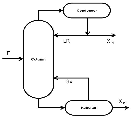
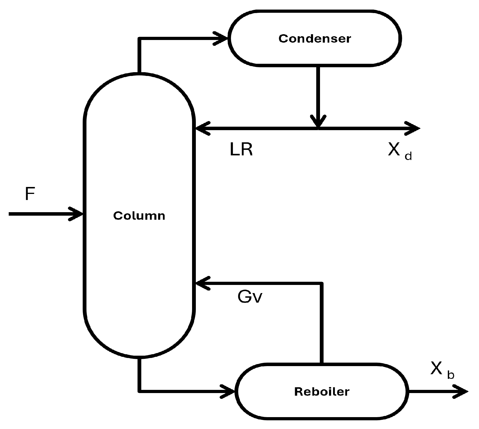
To demonstrate the effectiveness of the DEMM in a practical implementation, a binary distillation column has been selected as an industry-relevant nonlinear system [22]. A schematic representation of the system is shown in Figure 1. In a binary distillation column, there are two outputs to be controlled (which is why such systems are often referred to as two-product distillation columns): a top distillate product, which is vaporized and subsequently condensed, and a bottom product component, which can be reboiled to improve its purity.

Figure 1. Schematic of a binary distillation column.

For this particular example, the Wood and Berry binary distillation model [23] is selected, as it was derived from operating distillation columns and is representative of many chemical process control systems.

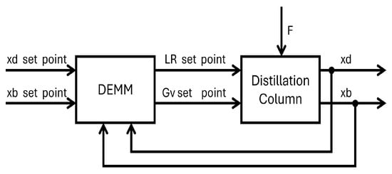
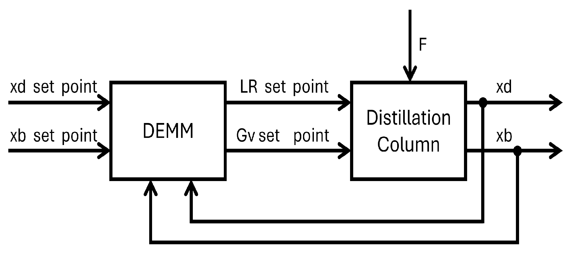
Figure 2 shows a block diagram of the proposed DEMM used to control the distillation column. A mathematical model of a binary distillation column, based on several simplifying assumptions, is employed in this work. In developing the model, the liquid hold-up in the reflux drum and at the base of the column is assumed to be constant. It is also assumed that the distillate composition is controlled by manipulating the reflux flow rate, while the bottom product composition is controlled by adjusting the boil-up rate.

Figure 2. Control loop of the distillation column using the proposed DEMM.

Boil-up control is typically achieved by varying the steam flow to the reboiler. In the mathematical model, the dynamics of the heat transfer processes in the condenser and the reboiler are neglected, since in commercial-scale columns the dynamic response of these heat exchangers is usually much faster than that of the column itself. For multivariable systems such as distillation columns with multiple delays, a commonly used model takes the form:

$$\left[\begin{array}{c}{X}_d\left(s\right)\\ X_b\left(s\right)\end{array}\right]=\left[\begin{array}{cc}{\displaystyle \frac{12.8 e^{-s}}{16.7s+1}}& {\displaystyle \frac{-18.9 e^{-3s}}{21s+1}}\\ {\displaystyle \frac{6.6 e^{-7s}}{10.9s+1}}& {\displaystyle \frac{-19.4 e^{-3s}}{14.4s+1}}\end{array}\right]\left[\begin{array}{c}LR\left(s\right)\\ Gv\left(s\right)\end{array}\right]+\left[\begin{array}{c}{\displaystyle \frac{3.8 e^{-8.1s}}{14.9s+1}}\\ {\displaystyle \frac{4.9 e^{-3.4s}}{13.2s+1}}\end{array}\right]F\left(s\right)$$

(55)

where $X_d\left(s\right)$ is the distillate composition, $X_b\left(s\right)$ is the bottom-product composition, $LR\left(s\right)$ is the reflux flow rate, $Gv\left(s\right)$ is the steam-flow rate supplied to the reboiler, and $F\left(s\right)$ represents the feed-flow disturbance. This transfer function was determined experimentally by Wood and Berry around a steady-state operating point [23], defined as follows (these same values will be considered for the following implementation examples, unless otherwise stated):

$$\begin{array}{cc}& X_d (\mathrm{overhead} \mathrm{composition} \mathrm{of} \mathrm{the} \mathrm{distillate})=96.25 \mathrm{mol}\%\hfill \\ & X_b (\mathrm{composition} \mathrm{of} \mathrm{the} \mathrm{bottom} \mathrm{products})=0.5 \mathrm{mol}\%\hfill \\ & LR (\mathrm{reflux} \mathrm{drum} \mathrm{flow} \mathrm{rate})=0.0147 \mathrm{kg}/\mathrm{s}\hfill \\ & Gv (\mathrm{steam} \mathrm{flow} \mathrm{rate})=0.0129 \mathrm{kg}/\mathrm{s}\hfill \\ & F (\mathrm{feed} \mathrm{rate})=0.0185 \mathrm{kg}/\mathrm{s}\hfill \end{array}$$

For model identification purposes, Gaussian white-noise excitation signals following a normal distribution N(0,0.1), where 0 and 0.1 denote the mean and standard deviation, respectively, were applied to the model inputs. These excitation signals are used exclusively during the identification stage and should not be confused with the disturbance scenarios employed later in the closed-loop control studies. The following discrete models were obtained by applying a least-squares identification procedure to the input–output data:

$$X{d}_k-1.0458 X{d}_{k-1}+0.0965 X{d}_{k-2}=4.9182+0.0056 L{R}_{k-2}-0.0006 L{R}_{k-3}-0.0066 G{v}_{k-4}+0.0007 G{v}_{k-5}$$

(56)

The resulting mean squared prediction error is 0.048.

$$X{b}_k-1.3862 X{b}_{k-1}+0.4322 X{b}_{k-2}=0.6295+0.0044 L{R}_{k-8}-0.0021 L{R}_{k-9}-0.0098 G{v}_{k-4}+0.0045 G{v}_{k-5}$$

(57)

The resulting mean squared prediction error is 0.051. The corresponding incremental model is then given by:

$$\begin{array}{cc}\hfill X{d}_k-2.0458X{d}_{k-1}+1.1422X{d}_{k-2}-0.0965X{d}_{k-3}& =0.0056\mathsf{\Delta }L{R}_{k-2}-0.0006\mathsf{\Delta }L{R}_{k-3}-0.0066\mathsf{\Delta }G{v}_{k-4}+0.0007\mathsf{\Delta }G{v}_{k-5}\hfill \\ \hfill X{b}_k-2.3862X{b}_{k-1}+1.8185X{b}_{k-2}-0.4322X{b}_{k-3}& =0.0044\mathsf{\Delta }L{R}_{k-8}-0.0021\mathsf{\Delta }L{R}_{k-9}-0.0098\mathsf{\Delta }G{v}_{k-4}+0.0045\mathsf{\Delta }G{v}_{k-5}\hfill \end{array}$$

(58)

The purpose of the identification stage was to obtain a predictive model suitable for controller design rather than to perform a comprehensive system-identification study. Consequently, the model quality was assessed using prediction-error measures, while a detailed validation campaign including residual analysis, cross-validation, and statistical consistency tests was not considered within the scope of the present work.

In the closed-loop simulations, the feed flow rate F is treated as an external disturbance acting on the process, whereas the desired distillate and bottom compositions constitute the reference signals. Disturbance-rejection tests therefore evaluate the controller response to variations in F, while setpoint-tracking tests evaluate the response to changes in the reference compositions.

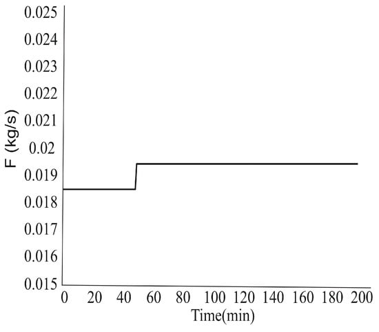
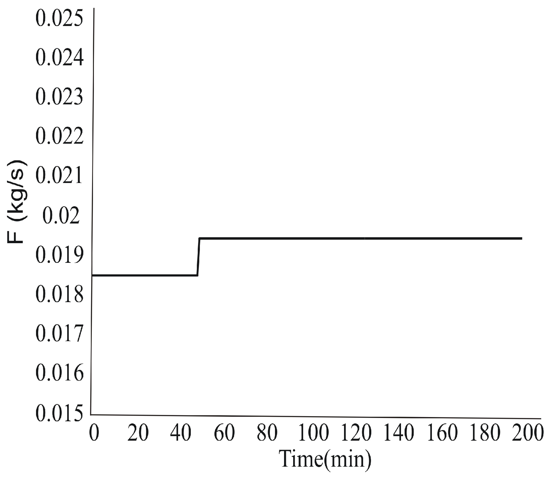
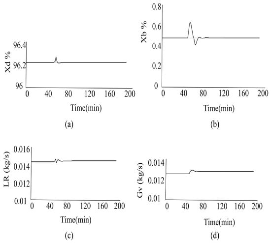
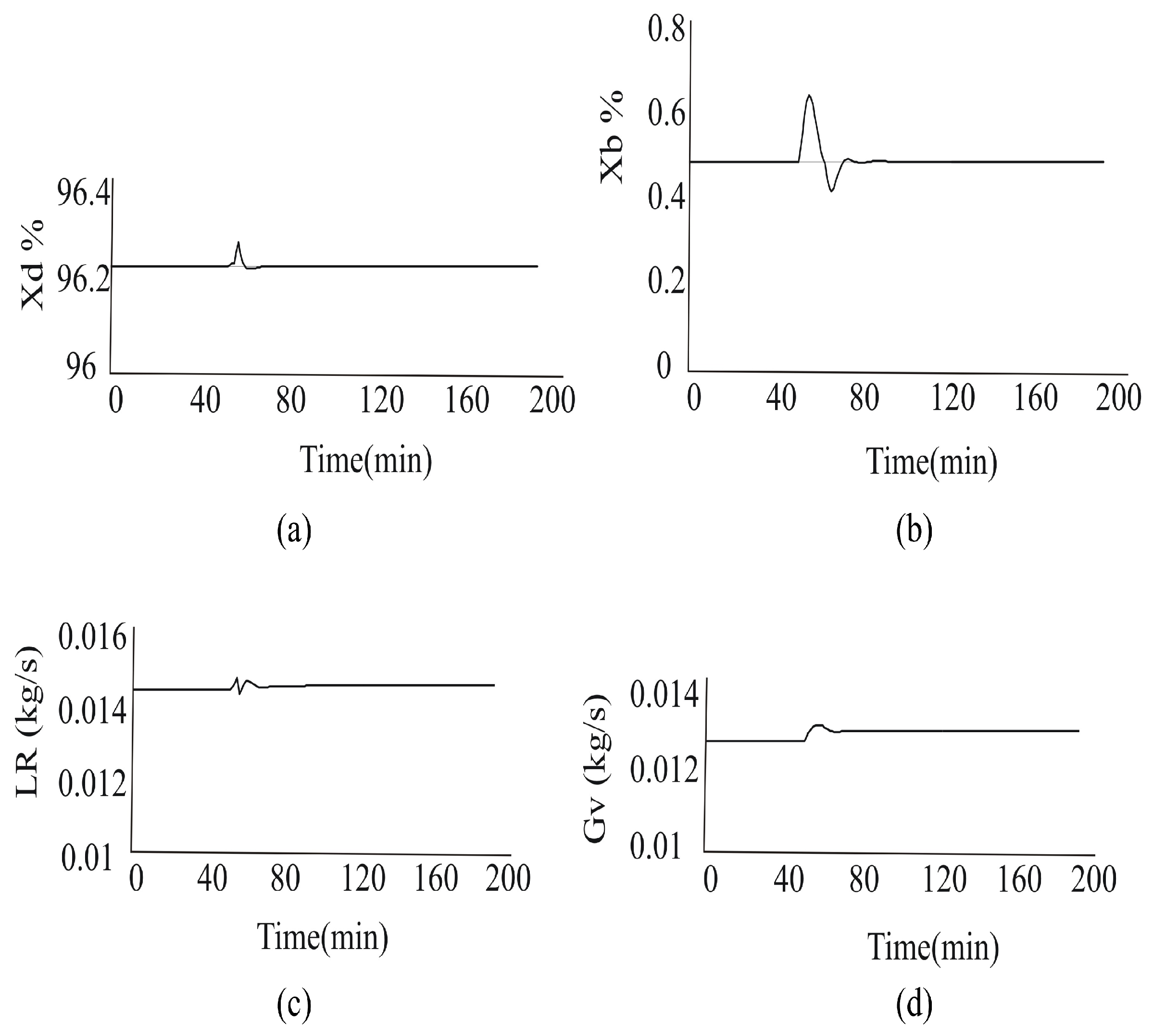
By applying DEMM with $h=15$, $Q_{Xd}=I$, $Q_{Xb}=10·I$, and $R=5·I$ (where I represents the identity matrix), and assuming a step disturbance of $F=5\%$ at the plant input, as shown in Figure 3. Figure 4 shows that the system exhibits satisfactory disturbance-rejection and setpoint-tracking performance.

Figure 3. Step disturbance of $F=5\%$ at the plant input.

Figure 4. Disturbance-rejection response of the DEMM controller to a +5% step change applied to the feed-flow disturbance F at t = 50 min. Reference compositions remain constant during the experiment: (a) overhead composition of the distillate, (b) composition of the bottom products, (c) reflux drum flow rate, and (d) steam flow rate.

In the response plots, the reference trajectories are represented together with the corresponding controlled outputs to facilitate the evaluation of tracking performance and disturbance rejection.

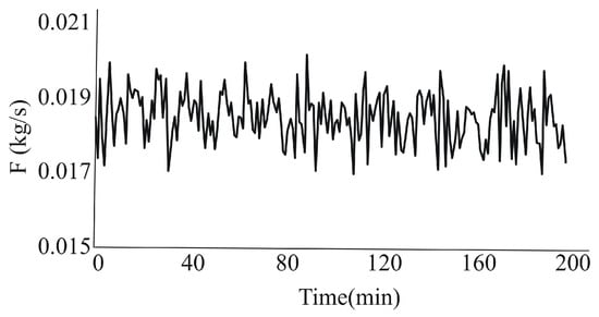
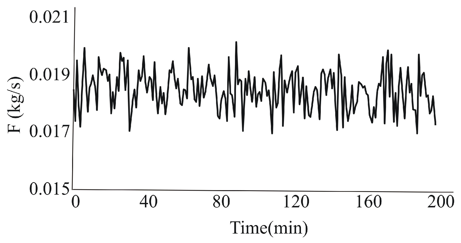
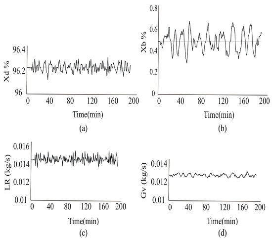
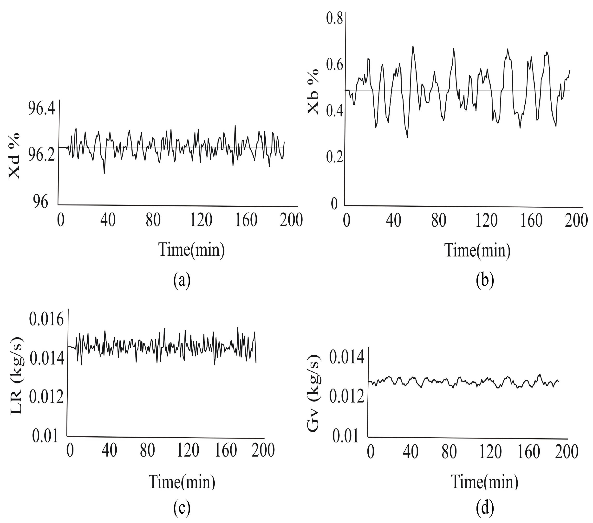
Next, consider the presence of noise $N(0,0.1)$ in F at the plant input, as shown in Figure 5. The corresponding response of the outputs and control actions is presented in Figure 6a–d. The results indicate that the proposed controller maintains acceptable closed-loop performance in the presence of the tested disturbances and noise conditions.

Figure 5. Noise $N(0,0.1)$ applied at the plant input.

Figure 6. Disturbance-rejection response of the DEMM controller under Gaussian white-noise perturbations applied to the feed-flow disturbance F. Reference compositions remain constant during the experiment: (a) overhead composition of the distillate, (b) composition of the bottom products, (c) reflux drum flow rate, and (d) steam flow rate.

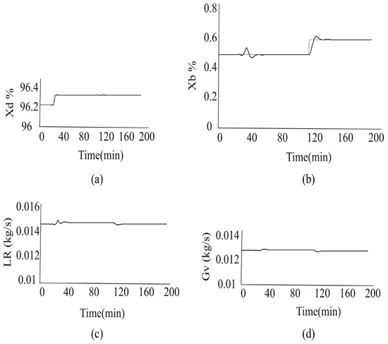
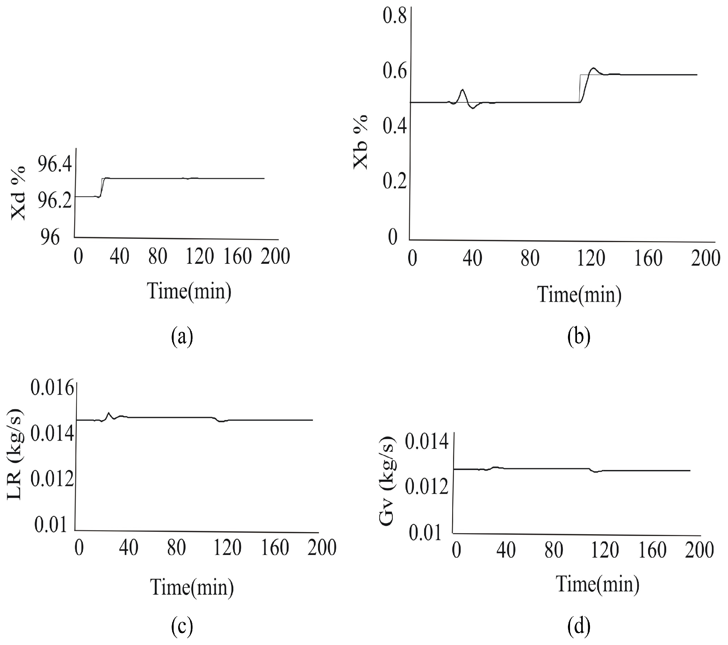
Successive step changes of amplitude 0.1 were applied to the distillate and bottom-composition reference signals in order to evaluate the setpoint-tracking performance of the controller. The transient response of the outputs and control actions of the column, under these reference changes, is shown in Figure 7a–d.

Figure 7. Setpoint-tracking response of the DEMM controller to successive reference changes in the desired distillate and bottom compositions: (a) overhead composition of the distillate, (b) composition of the bottom products, (c) reflux drum flow rate, and (d) steam flow rate.

The results indicate satisfactory disturbance-rejection and setpoint-tracking performance under the scenarios considered. The simulation results suggest that the proposed controller provides a reasonable trade-off between smooth reference tracking and disturbance rejection under the operating conditions considered.

5. Conclusions

This work has presented the application of the DEMM control algorithm, a predictive control strategy, to a binary distillation column. The proposed DEMM should be regarded as an input–output predictive control formulation derived from discrete difference equations rather than as a fundamentally different predictive control paradigm. The proposed approach achieves smooth control responses while the theoretical comparison presented in this work indicates that DEMM requires a more compact model parameterization than the DMC formulation considered in this work. The present work does not address formal stability guarantees or offset-free MPC formulations incorporating disturbance estimation. These aspects constitute potential directions for future research. Simulation results under noise and disturbance conditions demonstrate that DEMM effectively attenuates disturbances while maintaining stable and smooth closed-loop performance. Overall, the proposed controller provides a practical and efficient solution for enhancing the performance of distillation processes. The simulations presented in this work are intended to illustrate the controller behavior under representative operating conditions. A comprehensive robustness assessment involving model uncertainty, repeated stochastic realizations, and comparative benchmarking is beyond the scope of the present study.

The present formulation focuses on the unconstrained predictive control problem. The incorporation of actuator and output constraints through quadratic-programming-based optimization, together with formal stability analysis and robustness studies under model uncertainty, constitutes an interesting direction for future work.

References

- Schwenzer, M.; Ay, M.; Bergs, T.; Abel, D. Review on model predictive control: An engineering perspective. Int. J. Adv. Manuf. Technol. 2021, 117, 1327–1349. [Google Scholar] [CrossRef] [Scilit]
- Yao, Y.; Shekhar, D.K. State of the art review on model predictive control (MPC) in Heating Ventilation and Air-conditioning (HVAC) field. Build. Environ. 2021, 200, 107952. [Google Scholar] [CrossRef] [Scilit]
- Sun, Z.; Wu, B.; Wang, D.; Chen, J. Event-triggered model predictive control of spacecraft formation. IEEE Trans. Autom. Sci. Eng. 2024, 22, 7696–7711. [Google Scholar] [CrossRef] [Scilit]
- Xiao, H.; Zhao, D.; Gao, S.; Spurgeon, S.K. Sliding mode predictive control: A survey. Annu. Rev. Control 2022, 54, 148–166. [Google Scholar] [CrossRef] [Scilit]
- Salzmann, T.; Kaufmann, E.; Arrizabalaga, J.; Pavone, M.; Scaramuzza, D.; Ryll, M. Real-time neural mpc: Deep learning model predictive control for quadrotors and agile robotic platforms. IEEE Robot. Autom. Lett. 2023, 8, 2397–2404. [Google Scholar] [CrossRef] [Scilit]
- Li, Y.; Liu, D.; Wu, T.; Guo, W.; Zhang, X.; Deng, Y. Model predictive current control for permanent magnet synchronous motor based on neural network. In 2023 IEEE International Conference on Predictive Control of Electrical Drives and Power Electronics (PRECEDE); IEEE: New York, NY, USA, 2023; pp. 1–6. [Google Scholar]
- Bharatiraja, C.; Deepak, M.; Krishnamurthy, M. Performance comparison of enhanced model predictive control and model predictive direct torque control in SRM drives. In 2024 IEEE Transportation Electrification Conference and Expo (ITEC); IEEE: New York, NY, USA, 2024; pp. 1–6. [Google Scholar]
- Clarke, D.; Mohtadi, C.; Tuffs, P. Generalized predictive control—Part I. The basic algorithm. Automatica 1987, 23, 137–148. [Google Scholar] [CrossRef] [Scilit]
- Camacho, E.; Bordons, C. Model Predictive Control; Advanced Textbooks in Control and Signal Processing; Springer: London, UK, 2004. [Google Scholar]
- Cutler, C.; Ramaker, B. Dynamic matrix control. In Proceedings of the A Computer Control Algorithm. In Joint Automatic Control Conference, San Francisco, CA, USA, 13–15 August 1980; Volume 17, p. 72. [Google Scholar]
- Zhou, X.; Dong, S.; Chen, X.; Zhao, J.; Wang, X. Dynamic matrix control based on PID controller design for engraving machine system. In 2023 35th Chinese Control and Decision Conference (CCDC); IEEE: New York, NY, USA, 2023; pp. 2251–2256. [Google Scholar]
- Wang, Y.; Cheng, Y.; Xiong, Y.; Yan, Q. Estimation of battery open-circuit voltage and state of charge based on dynamic matrix control-extended Kalman filter algorithm. J. Energy Storage 2022, 52, 104860. [Google Scholar] [CrossRef] [Scilit]
- Santos, T.L.; Normey-Rico, J.E. A generalised dynamic matrix control for unstable processes based on filtered predictions. ISA Trans. 2023, 136, 297–307. [Google Scholar] [CrossRef] [Scilit] [PubMed]
- Hong, S.; Bai, J.; Zou, H. An improved dynamic matrix control with output penalty for industrial processes. Can. J. Chem. Eng. 2025, 103, 4952–4967. [Google Scholar] [CrossRef] [Scilit]
- Sunori, S.K.; Mittal, A.; Sharma, S.; Saxena, A.K.; Nainwal, D.; Juneja, P. Controller Design with Dead Time Compensation for Distillation Column. In 2022 7th International Conference on Communication and Electronics Systems (ICCES); IEEE: New York, NY, USA, 2022; pp. 16–20. [Google Scholar]
- Gao, W.; Dong, C.; Bo, C.; Li, J.; Cao, W. Multivariable Dynamic Matrix Control Method for Distillation Process Based on Subspace System Identification. In 2023 CAA Symposium on Fault Detection, Supervision and Safety for Technical Processes (SAFEPROCESS); IEEE: New York, NY, USA, 2023; pp. 1–6. [Google Scholar]
- Tahir, N.M.; Zhang, J.; Armstrong, M. Advancing control paradigms in heat-integrated distillation columns: An MPC perspective. In 2024 29th International Conference on Automation and Computing (ICAC); IEEE: New York, NY, USA, 2024; pp. 1–6. [Google Scholar]
- Herra, E.V.; Vásquez, M.C. A DMC implementation for a binary distillation column: A MIMO approach. In IEEE Biennial Congress of Argentina (ARGENCON); IEEE: New York, NY, USA, 2022; pp. 1–5. [Google Scholar]
- Zhang, X.; Zhou, K.; Li, H.; Xia, C.; Zhang, Z.; Liu, F. Control for Quality of the Separated Products of a Butylene-Butane Distillation Column Based on High Order Iterative Learning Control. In 2023 International Annual Conference on Complex Systems and Intelligent Science (CSIS-IAC); IEEE: New York, NY, USA, 2023; pp. 196–201. [Google Scholar]
- Tahir, N.M.; Zhang, J.; Armstrong, M. Genetic Algorithm Optimization based Control for Heat Integrated Distillation Column. In 2025 22nd International Learning and Technology Conference (L&T); IEEE: New York, NY, USA, 2025; Volume 22, pp. 77–82. [Google Scholar]
- Wang, C.; Zhuang, Y.; Dong, Y.; Zhang, L.; Liu, L.; Du, J. Design and control analysis of the side-stream extractive distillation column with low concentration intermediate-boiling entrainer. Chem. Eng. Sci. 2022, 247, 116915. [Google Scholar] [CrossRef] [Scilit]
- Sivakumar, R.; Manic, K.S.; Nerthiga, V.; Akila, R.; Balu, K. Application of fuzzy model predictive control in multivariable control of distillation column. Int. J. Chem. Eng. Appl. 2010, 1, 38. [Google Scholar] [CrossRef] [Scilit]
- Wood, R.; Berry, M. Terminal composition control of a binary distillation column. Chem. Eng. Sci. 1973, 28, 1707–1717. [Google Scholar] [CrossRef] [Scilit]
Disclaimer/Publisher’s Note: The statements, opinions and data contained in all publications are solely those of the individual author(s) and contributor(s) and not of MDPI and/or the editor(s). MDPI and/or the editor(s) disclaim responsibility for any injury to people or property resulting from any ideas, methods, instructions or products referred to in the content. |
© 2026 by the authors. Licensee MDPI, Basel, Switzerland. This article is an open access article distributed under the terms and conditions of the Creative Commons Attribution (CC BY) license.