


Abstract
The trajectory tracking problem of underactuated unmanned surface vehicles (USVs) with unknown physical parameters arising from hydrodynamic effects is addressed using a robust control strategy based on a sliding-mode dynamic neural network identifier. To handle the unknown physical parameters, a dynamic neural network identifier with a novel structure is developed, enabling the construction of an equivalent mathematical model of the USV dynamics. To compensate for the underactuated nature of the system, a coordinate transformation is introduced. Using this transformation, together with the proposed identifier, a nonsingular sliding-mode controller is designed. Lyapunov-based analysis establishes finite-time convergence of the neural weight estimation errors to zero and convergence of the identification errors to a bounded neighborhood of zero. Furthermore, once the identification errors enter this bounded region, they asymptotically converge to zero. In addition, the closed-loop stability analysis guarantees finite-time convergence of the tracking errors. The effectiveness of the proposed identifier–controller framework is validated through simulation studies that incorporate explicit actuator saturation constraints and external disturbances to emulate realistic operating conditions. These results demonstrate the practical applicability of the proposed control strategy, as the commanded inputs remain within the physical limits of the propulsion system. Comparative results with a state-of-the-art model-based super-twisting controller show that the proposed approach achieves comparable tracking performance while eliminating the need for prior knowledge of the system’s dynamic parameters.
1. Introduction
Autonomous maneuvering of unmanned surface vehicles (USVs) requires control of the heading angle and the horizontal position to carry out accurate trajectory tracking tasks [1]. This type of vehicle is subject to complex aquatic environments, internal nonlinearities, actuator saturation effects and dead zones, modeling and parametric uncertainties, and external disturbances including wind, waves, and currents, among others [2]. In this context, one of the most challenging issues is determining the so-called hydrodynamic coefficients, which are the physical parameters related to hydrodynamic phenomena. These numerical values characterize the damping and added-mass effects experienced by the USV.
Hydrodynamic coefficients are commonly estimated on the basis of a set of simplifying modeling and physical assumptions. Several procedures and techniques have been developed to deal with this issue, for example, computational fluid dynamics, analytical and semi-empirical methods, or captive and free model testing [3]. However, in most cases, the more accurate and complete the USV model is, the more complicated it is to perform a parametric identification of these coefficients.
The authors in [4] presented the identification of a maneuvering unmanned marine vehicle. Such identification is based on the use of an extended Kalman filter and a support vector machine, avoiding an experimental method. In [5], the authors deal with the identification of the hydrodynamic coefficients of an underwater vehicle. The identification is based on a simplified identification model considering low complexity approximations of the damping effects.
In most cases, it is difficult to realize a parametric identification due to complex mathematical representations of mechanical systems (including coupled, underactuated, or lumped parameter dynamics) or due to a priori nonlinear models not being available. In this case, an approximation of complex and/or unknown nonlinear expressions containing parametric uncertainties can be carried out using nonparametric identification. This scheme constructs an approximation directly from the input–output signals, without presuming any fixed or simple mathematical form.
The study in [6] introduces a novel nonparametric identification strategy of a ship maneuvering motion based on a combination of Gaussian process regression and a genetic algorithm. In the work reported in [7], a fixed-time extended state observer is designed to estimate environmental disturbances and model uncertainties affecting multiple surface vehicles in a distributed cooperative control problem. In [8], a finite-time disturbance observer is designed to approximate a nonlinear expression with uncertain damping and added mass coefficients of a USV model. Other studies have used optimal and intelligent strategies to deal with the identification of unknown USV dynamics. The strategy presented in [9] makes use of an optimal method to approximate the uncertainties and hydrodynamic couplings of the mathematical model of a USV. This strategy combines the particle swarm optimization algorithm with the interior-point algorithm.
The work in [10] proposes an adaptive fuzzy controller to address the path-tracking problem for a USV. The proposed scheme leverages the approximation capabilities of a fuzzy inference system to capture nonlinear dynamics, enabling the identification and compensation of model uncertainties and time-varying disturbances. Similarly, in [11], the authors develop a course-tracking control strategy for USVs that incorporates actuator input quantization. A fuzzy logic system is used to approximate system uncertainties, while closed-loop stability is rigorously ensured through a Lyapunov-based analysis. It is worth noting that an adequate estimation of the hydrodynamic interactions represents a key step in obtaining a faithful mathematical description to predict the USV motion performance as well as to design model-based control strategies to compensate for their influence and achieve robust trajectory tracking.
Another important issue related to the USV’s dynamic nature is its underactuated motion behavior. In this case, the lateral motion cannot be directly regulated because the vehicle is only equipped with actuators for surge and yaw movements; the lateral motion control requires a coordinated combination of the yaw and surge motions. This makes designing tracking controllers for underactuated USVs more difficult than for fully actuated USVs. In this respect, a model-based control strategy that has recently proven to be effective in addressing underactuated USV tracking problems is the so-called hand position point (HPP) approach [12,13,14,15,16,17]. This method makes use of a change of coordinates applied to the underactuated dynamic system to transform it into an actuated one, allowing the design of direct control strategies instead of the use of cascaded-based methods.
Nonlinear and classical controllers are designed based on such a simplified mathematical structure. In the study reported in [15], the authors focus on the design of a trajectory tracking and path following controller using the HPP strategy for marine vehicles. In [18], a time-varying version of the HPP is introduced for underactuated underwater vehicles that demonstrate its effectiveness in solving trajectory tracking problems. Similarly, in [16,17], sliding-mode controllers were implemented on HPP-based models to address trajectory tracking problems in USVs.
To address the approximation problem associated with parameter and modeling uncertainties, current studies employ dynamic neural network (DNN) architectures with higher structural complexity, for instance, the Hopfield-type state-space neural networks [19,20]. The continuous time evolution of this class of DNNs has proven to be effective in identifying unknown dynamics and uncertainties online in a broad variety of complex nonlinear systems [21,22,23,24,25,26]. Such DNNs have two key features: their tunable parameters (the synaptic weights) represent linear elements in the neural network structure, and their training is carried out using an online updating procedure that solves a set of differential equations.
In these studies, the identification stage is characterized by an asymptotic behavior of the identification error to an ultimately bounded region. Recent works based on such an identification scheme have succeeded in guaranteeing convergence rate conditions for the identification problem. In the work studied in [27], an exponential function-based learning law is designed for an identifier with the structure of the DNN described above. The DNN weights are updated by two adaptive algorithms that feature a specified exponential rate of convergence. The identification error is guaranteed to converge to an invariant set defined by a minimal ellipsoid. In addition, a finite-time convergence of the tracking error can be reached. The work in [28] proposes an adaptive sliding-mode controller with a DNN to identify and compensate for unknown hydrodynamic effects for an underwater vehicle. The DNN compensates for the unknown dynamics, and the sliding-mode control forces a finite-time convergence of the tracking error to zero. In this context, the identification error is only guaranteed to converge asymptotically to a bounded region, highlighting a key limitation in existing approaches. Addressing this issue remains an open problem and serves as a primary motivation for the developments presented in this work.
The main contributions of this manuscript are summarized as follows:
- A mathematical representation of the dynamics of the USV is developed using a novel nonparametric structure termed the sliding-mode-based dynamic neural network identifier (SM-DNNI). The proposed identifier structure is based on the DNN with a Hopfield-type state-space architecture reported in [21,22,23,24,25,26,27,28] with enhanced convergence properties provided by nonsingular terminal sliding-mode terms, and is driven by a sliding surface constructed from the identification errors between the measured USV states and the SM-DNNI outputs. This structure enables robust and adaptive online identification of the system dynamics without requiring prior knowledge of physical parameters. This identifier architecture, which integrates robustness and adaptation features, has not been previously reported in the literature.
- For the proposed SM-DNNI, a rigorous Lyapunov-based stability analysis is carried out for the identification error dynamics. This analysis establishes finite-time convergence of both the sliding surface and the weight estimation errors of the neural network to zero. Moreover, the identification errors between the SM-DNNI and the actual USV dynamics are shown to vanish in finite time. In contrast to the existing dynamic neural network identifiers reported in [21,22,23,28], which guarantee only asymptotic convergence to a bounded neighborhood of the origin, and the approach in [27], which ensures exponential convergence to a similar bounded region, the proposed method achieves finite-time convergence to zero.
- Building upon the proposed SM-DNNI framework, a nonsingular terminal sliding-mode controller is developed to address the trajectory tracking problem of USVs. A rigorous stability analysis demonstrates that the tracking errors between the SM-DNNI states and the reference trajectory converge to zero in finite time, while the tracking errors of the actual USV asymptotically approach zero. In particular, the proposed control strategy does not require prior knowledge of the physical parameters of the USV. Although a related adaptive closed-loop control architecture is presented in [28], where finite-time convergence of tracking error is achieved via sliding-mode control, the associated identification errors are only guaranteed to converge asymptotically to a bounded set. In contrast, the proposed approach guarantees finite-time convergence to zero for both the identification and tracking errors.
The remainder of the paper is organized as follows. Section 2 introduces the mathematical model of the USV and presents the preliminaries required for the stability analysis of the proposed methods. Section 3 describes the development of the robust nonparametric dynamic neural network identifier. Section 4 details the design of the control strategy. Simulation results under various scenarios, including actuator saturation and external disturbances, are presented in Section 5. Finally, Section 6 concludes the article and outlines directions for future research.
2. Preliminaries and Dynamic Model
This section introduces the mathematical concepts used in the stability analysis, as well as those that support the development of the nonparametric robust dynamic neural network identifier and the derivation of the proposed control strategy. The dynamic model of the underactuated surface vehicle is also described. Furthermore, based on the hand position point technique, introduced in [15], a mathematical model that represents the vehicle dynamics in the inertial frame for the coordinates x and y is derived.
2.1. Preliminaries
In the following, useful lemmas employed in the stability analysis for the identification and control strategies proposed in this manuscript are presented.
Lemma 1
([29]). Let , , …, and . Then
Lemma 2
([29]). Let , , …, and . Then
Lemma 3
([30,31]). Assume that there are positive constants , and . Consider that the Lyapunov function satisfies
Then, converges to zero in finite time, and the convergence time is given by
where is the initial condition of . Moreover, converges globally to zero in finite time if and only if and is radially unbounded.
2.2. Dynamic Model for the Surface Vehicle
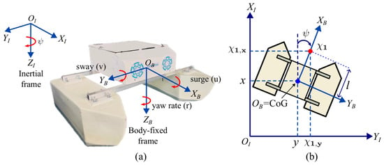
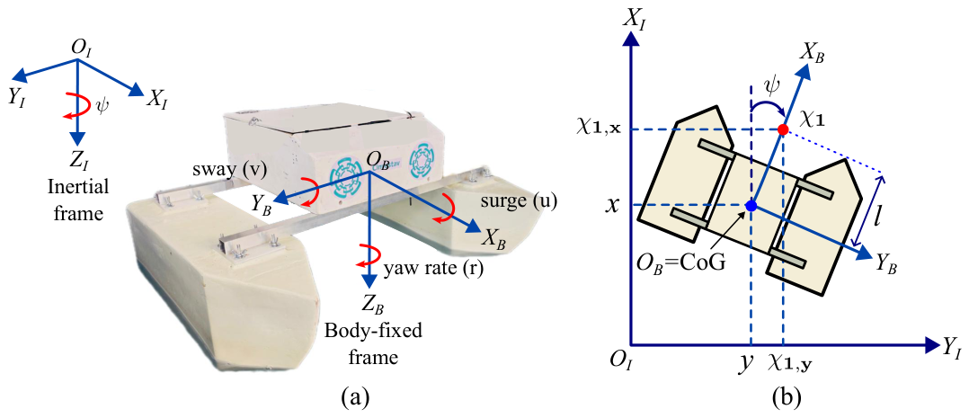
The following set of equations expresses a simplified mathematical model of the USV with three degrees of freedom (see Figure 1a): surge, sway, and yaw rate, introduced in [32,33,34]:
where x and y denote the position of the center of gravity (CoG) of the vehicle with respect to the inertial frame, while the yaw angle is denoted by . The variables u and v represent the surge and sway translational velocities in the body frame, respectively. Additionally, r denotes the angular yaw velocity (yaw rate). The external disturbances, primarily generated by the waves, are denoted by , , and . The control signals for the surge and yaw velocities are given by and , respectively. The functions , , as well as and , are defined as
where m is the mass of the vehicle and denotes the moment of inertia about the Z-axis. The hydrodynamic parameters associated with the linear damping are denoted by , , , while the nonlinear (quadratic) damping coefficients are given by , , . Finally, the added mass coefficients are defined as , and . Given the slow dynamics of the proposed USV, characterized by velocities on the order of 1 m/s, and the considered sampling interval of 0.001 s, the system exhibits a clear separation of time scales; therefore, a continuous-time model was adopted for the design of the control strategy.
Figure 1.
USV diagrams. (a) Reference frames, (b) hand position point in the horizontal plane.
To address the issue of underactuation evidenced by the dynamic model presented in (5), the HPP method used in [15,16,17] is applied. This method consists of defining the location of the HPP in the vehicle’s body (see Figure 1b), which corresponds to the transformation vector given by
where is a distance that enables us to represent a pivot point along the longitudinal axis. With this, the new variables to be controlled are and . The time derivative of is given as
Assuming the change of variables, let . Then, is given by
where the rotation matrix is defined as
By substituting the dynamic model presented in (5), one obtains the following result
Finally, for the surface vehicle, the state space dynamics are expressed in terms of and as
where
The dynamic model can be rewritten in modeling-error form as
where and represent the initial weights, and have the structure
The vector activation functions are composed of sigmoidal functions and have the following structure: and , where . Let us define . The elements of the vector of activation functions are defined as
where , , , , , , are parameters of the activation functions. Finally, the modeling error term, denoted by , is given as
Assumption 1.
The elements of the modeling error vector are bounded as and , where and are positive constants.
2.3. Identification Sliding Surface
Let us define the identification errors as , , where and represent the identification of and , respectively. Moreover, as outlined in [35], the following sliding surface for the identification errors is defined
where , , and are positive definite gain matrices. The function is defined as
for , where and . Let us define , where is the sign function. The time derivative of the sliding surface is given as
where
Solving the system of equations:
allows us to obtain the values of parameters and as
With the values computed for and , the sliding surface (17) remains continuous.
3. Nonparametric Robust Dynamic Neural Network Identifier
To identify the dynamics of the USV described in (14), the following SM-DNNI is proposed
where , and . The neural weights and have a structure similar to the initial weights defined in (15), i.e., , with , and , with . The matrices are positive diagonal matrices.The function is defined element-wise as .
From the system dynamics and identifier dynamics, the dynamics of the identification error are obtained as
where the identification errors of the neural weights are defined as and . Moreover, by substituting (24) into (19), we obtain the following:
Theorem 1.
Let Assumption 1 be satisfied. Consider the nonparametric neural network identifier defined in (23) for the transformed dynamics (12) of an unmanned surface vehicle. If the adaptive gains for the neural weights are chosen as
then, the sliding surface and the estimation errors in the neural weights converge to zero in a finite time given by defined in (48). From the sliding surface definition, the identification errors and converge in finite time to an arbitrarily small set bounded by in a finite time given by , where is defined in (55). Once inside this set, the identification errors converge asymptotically to zero.
Proof.
For the update laws (26) and (27), the matrices , and , , are positive definite diagonal matrices. The functions and are defined element-wise as
where are the elements of and are the elements of , . The stability proof of the theorem is divided into two steps. The first is for the sliding phase, and the second is for the reaching phase.
Step 1. Sliding phase. Consider the following Lyapunov candidate function
The time derivative is given as
Notice that
and
Then, Equation (31) yields
Notice that for the term , and based on the Assumption 1, it follows that
where , with and . Then, yields
Notice that can be rewritten as
then
Notice that
Then, from (45) and Lemma 1 the following is obtained for
Then, from inequality (43)
Finally, from Lemma 3, it is concluded that the sliding surface , and the errors in the neural weights and converge globally within a finite time , defined as
Step 2. Reaching phase. Having guaranteed , the performance of the system enters the reaching phase, i.e.,
From Equation (24), we obtain . By substituting this into (49), the following differential equation is obtained for the identification error :
Notice from Equations (17) and (63) that (50) is a continuous piecewise function. Therefore, the following two cases are analyzed.
Case A. In this case, the performance of (50) when , with , is analyzed, resulting in
where and . To analyze the stability of (51), the following Lyapunov candidate function is proposed
The time derivative is obtained as
From the inequality defined in Lemma 1, we obtain the following:
Notice that the exponent is restricted as . Therefore, from Lemma 3, we conclude that converges to zero in finite time , defined as
Furthermore, from the condition for defined in (63), it is also concluded that the identification error reaches an arbitrarily small set bounded by in a finite time given by .
Case B. In this case, the performance of the differential Equation (50) when , is analyzed, resulting in
where . To analyze the stability of the differential Equation (56), the following Lyapunov function is proposed
The time derivative is obtained as
From the inequality defined in Lemma 2, we obtain the following:
Notice that the exponent is restricted as . Therefore, for , we obtain the following:
4. Control Strategy Design
Considering that the identification errors converge in finite time to a small bounded set close to zero, for control design purposes, the mathematical model represented by the identifier given in (23) is used. Let us define the tracking errors as and . The dynamics of the tracking errors are defined as follows
The sliding surface for the tracking errors is defined as
where . The function is defined as
for , where and . The temporal derivative of (62) is obtained as
Substituting the tracking error dynamics (61) yields
Then, the following control signal is proposed
where , and are positive diagonal matrices.
Remark 1.
It is important to emphasize that the control law is designed based on the SM-DNNI defined in Equation (23), while it is applied to the USV dynamic model given in Equation (5). Accordingly, the control signal is formulated using the identification errors, the sliding surface associated with the identification errors, and the sliding surface associated with the tracking errors.
In order to assess the stability of the tracking errors between the reference signal and the SM-DNNI, the following Lyapunov candidate function is proposed:
The temporal derivative is obtained as
From Lemma 1 the following expression is obtained for :
Then, from Lemma 3, it is concluded that the tracking error between the reference signal and the SM-DNNI converges to zero in a finite time
Remark 2.
For the simulation analysis, the tracking error between the reference signal and the transformed coordinate is defined by as
5. Simulation Results
To observe the effectiveness of the nonparametric dynamic neural network identifier and the nonsingular terminal sliding-mode controller, simulations under saturation constraints in the control signal were conducted using the USV model given in Equation (5). Furthermore, scenarios with periodic external disturbances and with external disturbances generated by waves were considered to highlight the robustness of the proposed controller, thereby emphasizing the robust capability of the proposed strategy. Table 1 summarizes the USV’s parameters used in the simulation sets, as reported in [32].
Table 1.
Underwater surface vehicle parameters.
Table 2 lists the gains employed for the robust neural network identifiers, while Table 3 presents the gains used for the sliding-mode controller. The identifier gains were obtained using a low-performance controller, i.e., one designed from a coarse process model to collect identification data. Once the identifier gains yielded acceptable performance, the controller gains were subsequently tuned heuristically. A brief description of the tuning procedure for the SM-DNNI gains listed in Table 2 and Table 3 is provided in the next remark.
Table 2.
Gains of the robust neural network identifier.
Table 3.
Gains of the sliding-mode control strategy.
Note for practitioners: regarding the SM-DNNI algorithm tuning procedure, a set of parameters is adjusted by trial and error to perform effective identification and control of the unknown dynamics. The gains , , determine mostly the identifier performance in the reaching phase. There exists a trade-off when selecting its magnitude; it increases the convergence velocity to the sliding surface for the identification error, but also increments the chattering generated over the sliding surface. A similar procedure is followed for the gains , , , , , to define sliding surface for the tracking error. Gains , , , weigh the linear terms associated with the identification error vectors during the reaching phase and the sliding phase. Greater values contribute to the convergence of the identification errors, mainly in the sliding phase. The gains and are related to the learning rate. If the learning rate increments its value, the DNN learns faster, but it can introduce oscillations in the learning process; if it has lower values, it reflects slow learning, affecting the identifier’s performance. The matrix gains and multiply the identification errors of neural weights; their magnitude weighs these correction terms to force the weights to converge to their nominal values. The gains and weight the discontinuous terms to force the neural weights to the nominal ones in finite time. If the values are too large, they may lead to abrupt oscillations of the neural weights during the reaching phase. The elements of the initial weights were selected to be greater than because requires a greater approximation capacity as it is located in the inverse compensation term in (66), avoiding any singularity in the control law. The gains and are included in the tracking control, and their values are selected by trial and error in order to guarantee fast and stable dynamics for the tracking sliding surface (62). A more detailed description of the structure of the neural network used is presented in Appendix A.
In the simulation study, explicit actuator saturation constraints were imposed to reflect realistic operating conditions, with the surge force limited to and the yaw moment limited to . These saturation bounds highlight the practical applicability of the proposed control strategy, as the commanded inputs do not exceed the physical capabilities of the propulsion system. For example, the saturation bounds can be fulfilled using a propulsion system composed of two T500 thrusters from BlueRobotics [36], whose main specifications are summarized in Table 4. In particular, this propulsion configuration is capable of generating a maximum thrust of 315.6 N in the forward (FWD) direction and 205.8 N in reverse (REV) when operating at a nominal voltage of 24 V. Considering that the thrusters are located on the physical platform at a distance of 0.5 m from the CoG, the maximum torque that can be generated is 157.8 Nm in the forward (FWD) direction and 102.9 Nm in reverse (REV).
Table 4.
T500 thruster main specifications.
For comparison purposes, the performance of the control strategy proposed in this manuscript is compared with a super-twisting (ST)-based control law proposed in [17], which is defined as
where and are positive diagonal matrices of dimension . The corresponding sliding surface is defined as
with gains selected as and .
It is important to emphasize that the super-twisting-based control law is designed under the assumption that both the dynamic model structure and its parameters are known. In contrast, the purpose of the comparison is to demonstrate that a comparable level of tracking performance can be achieved using the proposed SM-DNNI strategy, even in the absence of prior knowledge of the system parameters.
The desired reference signal used in the simulations is given by
This trajectory consists of single sinusoidal terms with large amplitudes and fixed frequencies; it is smooth and varies slowly. Additionally, the presence of a bias along the Y axis allows the evaluation of offset compensation.
Three simulation scenarios are presented. First, the SM-DNNI-based sliding-mode control is evaluated in the absence of external disturbances. Then, periodic external disturbances are introduced. Finally, wave-induced disturbances that affect the performance of the USV are considered.
5.1. Simulation Free-Disturbances
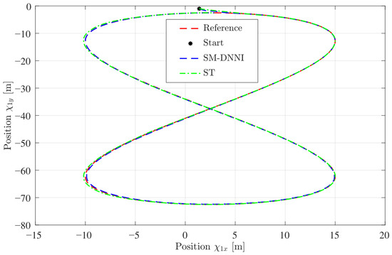
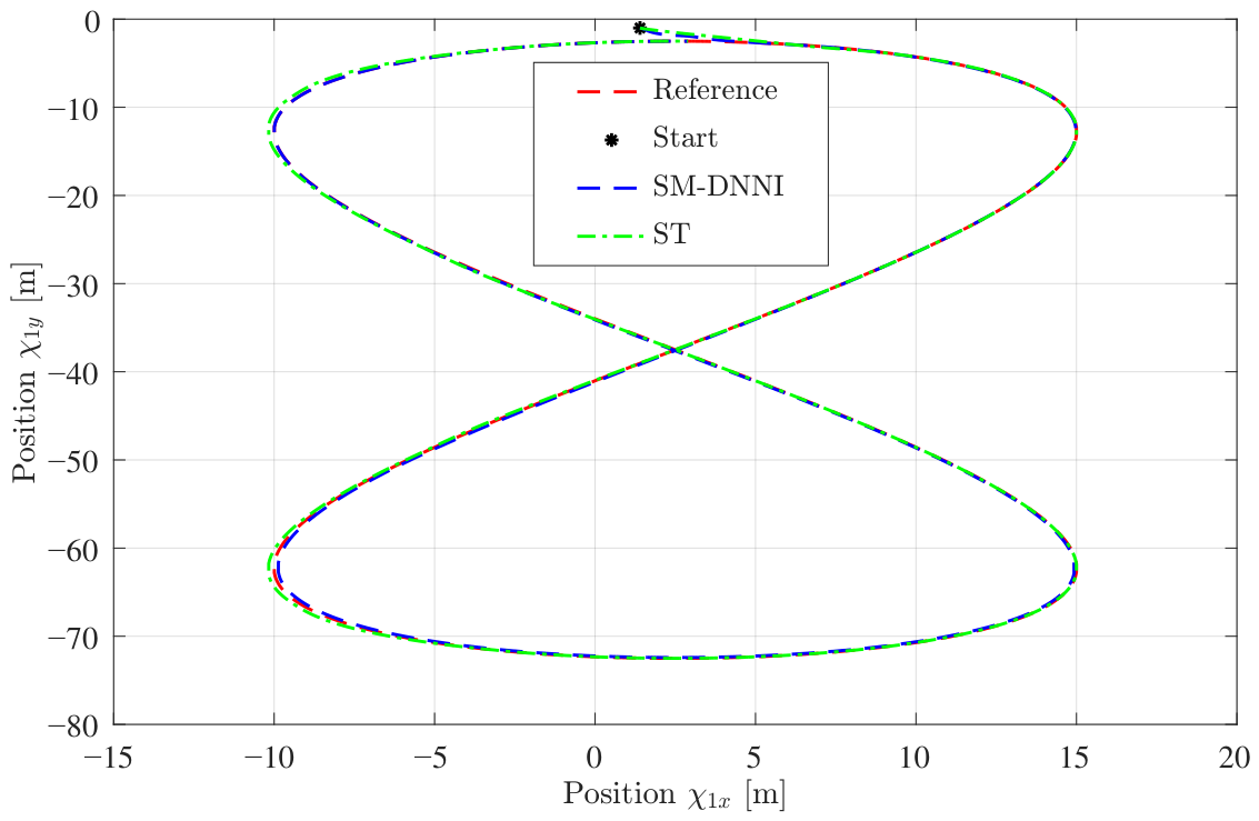
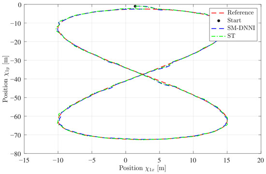
Figure 2 illustrates the trajectory tracking in the X–Y plane for the reference signal defined in Equation (75), obtained using the SM-DNNI and ST controllers under disturbance-free conditions and with saturation applied to the control signal.
Figure 2.
Trajectory tracking in the X-Y plane.
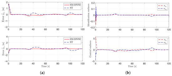
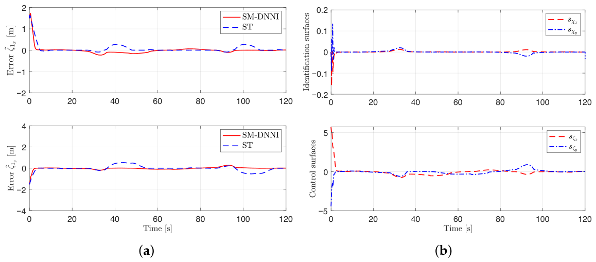
The corresponding tracking errors along the X and Y axes are presented in Figure 3a. Both the SM-DNNI and ST controllers track the reference signal with comparable settling times in the absence of disturbances. The ST controller was tuned under disturbance-free conditions and under saturation-free conditions to achieve performance comparable to, or exceeding, that of the controller defined in Equation (66), which is based on the SM-DNNI. Figure 3b presents the sliding surface of the neural network identification errors and the sliding surfaces of the neural controller along the X and Y axes, respectively. It can be seen that both sliding surfaces practically converge in finite time to a bounded region near zero.
Figure 3.
(a) Trajectory tracking errors in the X (Top), and Y (Bottom) axes for the SM-DNNI and the ST controllers. (b) Sliding surface of the neural network identification errors (Top), and sliding surfaces of the neural controller under external disturbances, along the X and Y axes (Bottom).
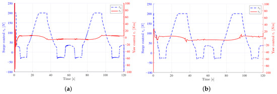
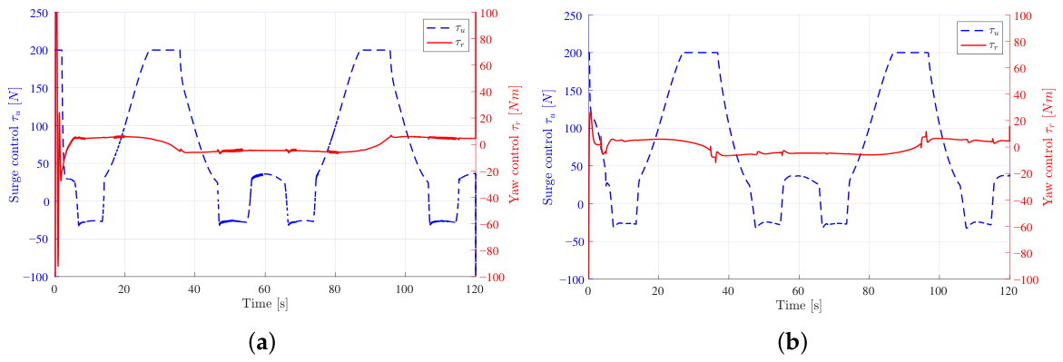
Figure 4 presents the control inputs for the surge and yaw dynamics, as defined in Equation (66), under actuator saturation conditions. The results indicate that both inputs remain within acceptable limits for the actuators of the unmanned surface vehicle.
Figure 4.
Control signals with actuator saturation for the surge and yaw dynamics. (a) SM-DNNI controller, (b) ST controller.
5.2. Simulations Under Periodic Disturbances
The periodic disturbances used to analyze the robustness of the proposed control strategy are given as follows
where amplitudes , , , are defined in Table 5 for two different cases.
Table 5.
Performance indices for periodic external disturbances. The values in bold represent the smallest tracking error in each case.
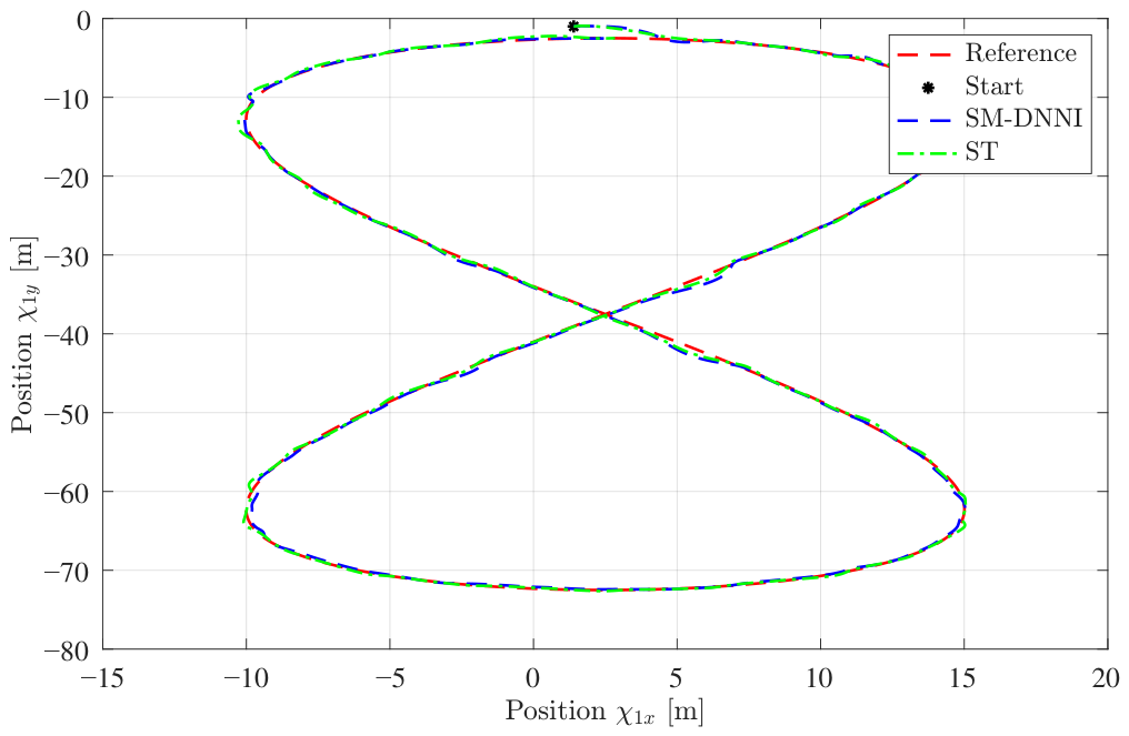
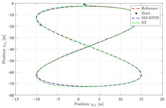
Figure 5 illustrates the trajectory tracking performance in the X–Y plane for the reference signal defined in Equation (75), using the SM-DNNI and ST controllers under disturbance conditions. Both controllers achieve satisfactory tracking; however, the SM-DNNI controller demonstrates improved accuracy, as evidenced by its reduced deviation from the desired trajectory compared to the ST controller.
Figure 5.
Trajectory tracking in the X-Y plane under periodic disturbances.
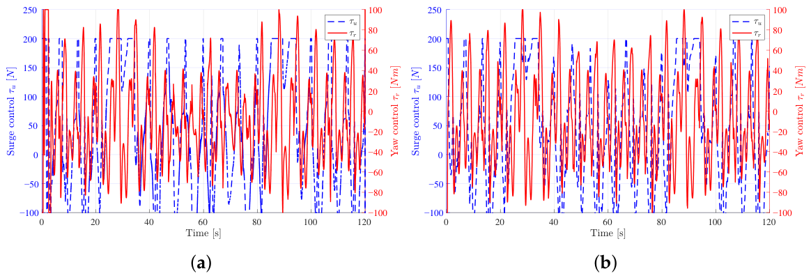
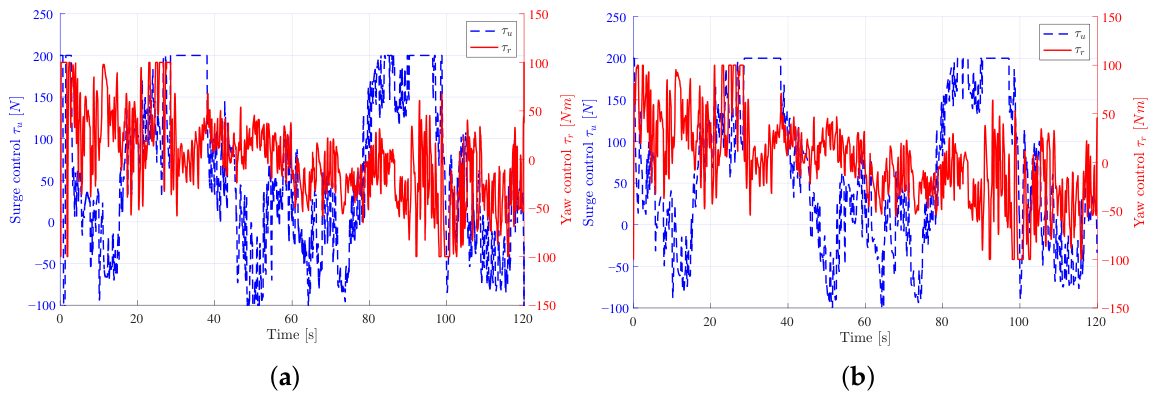
Figure 6 presents the control inputs for the surge and yaw dynamics, as defined in Equation (66) under external disturbances. The results indicate that both inputs remain within acceptable limits for the actuators of the unmanned surface vehicle. Note that the oscillations observed in the control inputs are primarily caused by the external disturbances introduced in the simulation. Nevertheless, the controller effectively compensates for these disturbances, maintaining satisfactory tracking performance.
Figure 6.
Control signals under actuator saturation and periodic disturbances for the surge and yaw dynamics. (a) SM-DNNI controller, (b) ST controller.
Table 5 summarizes the results obtained by applying the ISE, IAE, and ITAE performance indices to the simulation data.
Case 1 corresponds to the scenario without control signal saturation and in the absence of external disturbances. In this scenario, the super-twisting controller outperforms the proposed approach in two of the indices evaluated. However, when saturation is introduced in the control signal, the proposed method demonstrates improved handling, as reflected in Case 2, where all performance indices are lower than those of the super-twisting controller.
When control signal saturation is present, and periodic external disturbances are included in the simulation, the proposed approach achieves slightly better performance than the super-twisting controller, as shown in Cases 3 and 4. Overall, the identifier–controller strategy presented in this manuscript provides superior robustness against control signal saturation and periodic external disturbances in the USV, compared to a state-of-the-art model-based robust control approach.
5.3. Simulations Under Wave-Induced Disturbances
Given that the wave-induced interference forces acting on unmanned surface vehicles depend on both the wave characteristics and the vehicle’s motion state, the corresponding disturbance model is expressed as [37,38]
where L, T, and are the length, width, and draught of the USV and are defined in Table 1, is the seawater density, and is called the encounter angle, defined as the angle between the direction of the wave and the course of the USV. The wave energy is denoted by , defined as
where is the encounter frequency, is the wave amplitude, is the wavelength, and is the randomly distributed phase on .
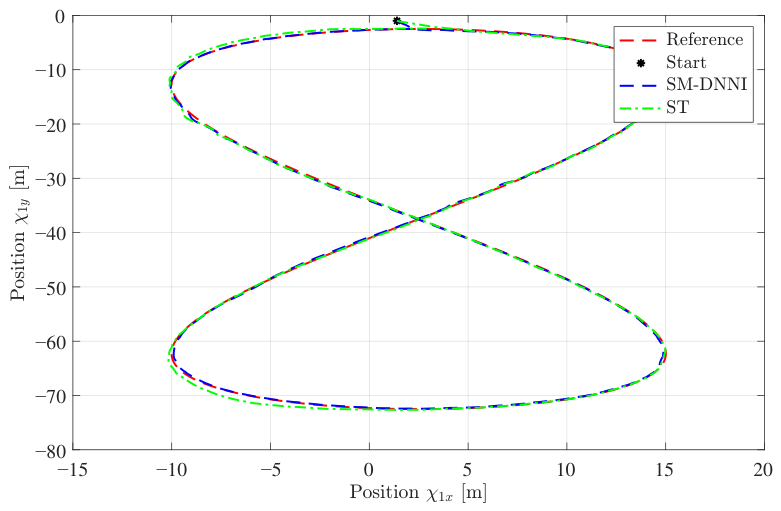
Figure 7 presents the trajectory tracking in the X–Y plane for the reference signal defined in Equation (75), using the SM-DNNI and ST controllers under wave-induced disturbances. The effects of the external disturbances can be observed in some regions of the X-Y plane, where slight oscillations are present in the upper-left region. Moreover, when the ST controller is used, the vehicle’s trajectory exhibits greater deviations from the desired trajectory than those observed with the SM-DNNI approach, particularly in the upper-left and lower-left regions.
Figure 7.
Trajectory tracking in the X-Y plane under wave-induced disturbances.
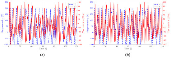
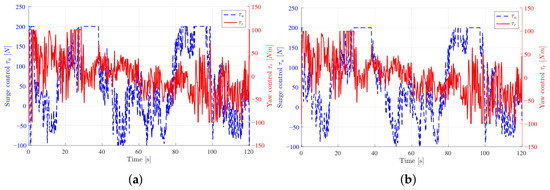
Figure 8 illustrates the control inputs for the surge and yaw dynamics, as defined in Equation (66), under conditions of control signal saturation and wave-induced disturbances. The results show that both inputs remain within the maximum limits imposed by the USV actuators. Compared with Figure 6, the oscillations observed in the control signals exhibit higher-frequency variations, which are necessary to effectively compensate for the effects of wave-induced disturbances, preserving satisfactory tracking performance.
Figure 8.
Control signals under actuator saturation and wave-induced disturbances for the surge and yaw dynamics. (a) SM-DNNI controller, (b) ST controller.
Table 6 presents the evaluation of the ISE, IAE, and ITAE performance indices in the presence of wave-induced disturbances affecting the USV. The simulations consider three wave amplitudes: m, m, and m. For each amplitude, ten simulations were performed, and the corresponding average performance indices are reported for each controller.
Table 6.
Performance indices for wave-induced disturbances. The values in bold represent the smallest tracking error in each case.
Across all wave conditions, the proposed identification–control strategy consistently demonstrates superior performance compared to the super-twisting controller.
5.4. Control Effort Analysis
Table 7 and Table 8 present the control effort comparison obtained from the numerical simulations. The control effort in surge and yaw is quantified as the sum of the absolute values of the corresponding control inputs.
Table 7.
Control effort for periodic external disturbances. The values in bold represent the larges control effort in each case.
Table 8.
Control effort for wave-induced forces. The values in bold represent the larges control effort in each case.
Table 7 summarizes the results for both disturbance-free simulations and simulations under periodic disturbances. In the disturbance-free scenario (Case 1), the super-twisting controller yields a higher control effort than the SM-DNNI controller, which is consistent with the reduced tracking error observed when the control input is not subject to saturation.
When control saturation is present (Cases 2–4), the SM-DNNI controller exhibits a higher control effort, in agreement with its improved tracking performance compared to the super-twisting controller. Furthermore, in Cases 3 and 4, the presence of disturbances leads to a significant increase in yaw control effort relative to Cases 1 and 2, due to the additional compensation required to maintain accurate tracking of the reference trajectory.
Table 8 summarizes the control effort under wave-induced disturbances. For most wave amplitudes, the SM-DNNI controller shows slightly higher control effort than the ST controller, consistent with its lower tracking error (Table 6). While the surge control effort increases moderately with wave amplitude, the yaw control effort approximately doubles with each increment, indicating the increased compensation needed to mitigate wave effects.
6. Conclusions
This study investigated the trajectory tracking problem of USVs in the presence of model uncertainties, unknown parameters, external disturbances, and actuator saturation. A novel dynamic neural network identifier was developed using a nonsingular sliding variable constructed from identification errors. Rigorous stability analysis demonstrated finite-time convergence of both the identification errors and neural network weights, yielding improved stability properties compared to existing dynamic neural network identification approaches. The information generated by the proposed identifier was further integrated into a sliding-mode control framework to achieve nonlinear feedback compensation of unknown USV dynamics and environmental disturbances. The resulting nonsingular sliding-mode controller guarantees finite-time convergence of the tracking errors to zero. Consequently, the closed-loop system that combines the dynamic neural network identifier and the sliding-mode controller effectively addresses the trajectory tracking problem for USVs operating under partially unknown and highly nonlinear conditions.
Based on the results obtained, the effectiveness of the proposed identifier–controller framework has been validated through simulation studies in which actuator saturation constraints and external disturbances representative of realistic operating conditions were explicitly incorporated. The practical applicability of the control strategy has been confirmed, as the control inputs were consistently maintained within the physical limits of the propulsion system. Furthermore, comparative analysis with a state-of-the-art model-based super-twisting controller has demonstrated that the proposed framework achieves comparable tracking performance while eliminating the requirement for prior knowledge of the system’s dynamic parameters.
Future work will focus on the experimental implementation of the proposed identifier–controller scheme to further assess its practical performance and robustness under real-world operating conditions.
Author Contributions
Conceptualization, F.M.P., E.S.E., and J.S.C.-R.; methodology, E.S.E.; software, J.P.O.O. and L.R.G.C.; validation, F.M.P. and J.S.C.-R.; formal analysis, F.M.P. and E.S.E.; investigation, F.M.P., E.S.E., and J.S.C.-R.; resources, O.G.-S. and L.R.G.C.; writing—original draft preparation, F.M.P., J.S.C.-R., and E.S.E.; writing—review and editing, F.M.P., E.S.E., J.P.O.O., O.G.-S., and L.R.G.C.; visualization, J.S.C.-R., J.P.O.O., and O.G.-S.; supervision, O.G.-S. and L.R.G.C.; funding acquisition, F.M.P. and L.R.G.C. All authors have read and agreed to the published version of the manuscript.
Funding
This research received no external funding.
Data Availability Statement
The raw data supporting the conclusions of this article will be made available by the authors upon request.
Acknowledgments
This work has been partially supported by the Mexican Secretariat of Science, Humanities, Technology, and Innovation.
Conflicts of Interest
The authors declare no conflicts of interest.
Abbreviations
The following abbreviations are used in this manuscript:
| USV | Unmanned Surface Vehicle |
| RBFNN | Radial Basis Function Neural Networks |
| HPP | Hand Position Point |
| ANN | Artificial Neural Network |
| DNN | Dynamic Neural Network |
| SM-DNNI | Sliding-Mode–based Dynamic Neural Network Identifier |
| CoG | Center of Gravity |
| DoF | Degree of Freedom |
| ST | Super-Twisting |
| REV | Reverse Direction |
| FWD | Forward Direction |
| ISE | Integral Square Error |
| IAE | Integral Absolute Error |
| ITAE | Integral Time-weighted Absolute Error |
Appendix A. Neural Network Structure
Appendix A.1. Architecture
The neural network architecture of the proposed SM-DNNI strategy is given in Equation (23):
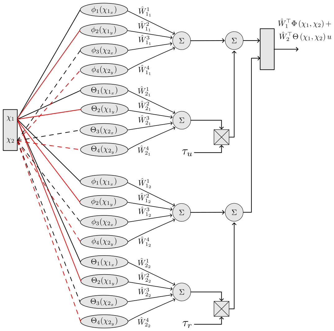
The underlined expression in Equation (A1) represents the neural network structure within the proposed identifier. A detailed description of the neural network architecture is provided in Figure A1. The network consists of an input layer that receives the state vector components (, ), a hidden layer composed of sixteen neurons with sigmoidal activation functions, and an output layer formed by a weighted sum of these activation functions through sixteen neural weights. Additionally, the input signal components and are included as external inputs, completing the series-parallel identification structure of the SM-DNNI.
Figure A1.
Neural network architecture of the SM-DNNI strategy. The input layer has four inputs: (black solid line), (red solid line), (black dotted line), (red dotted line).
Appendix A.2. Training Procedure
The training procedure is conducted in two steps: offline training and online adaptation.
- Offline training. The offline training procedure is performed to estimate the initial neural weights and . To obtain these weights, the nominal dynamics are given byNote that this equation does not include the term . Using a training dataset containing the state variables and , together with the control input , a least-squares algorithm is used to estimate the initial neural weights.
- Online adaptation. The online adaptation stage is performed during the simulation of the closed-loop dynamics, which include the USV dynamics, the SM-DNNI, and the control law. In this step, the identifier proposed in Equation (23) is used, while the neural weights are updated according to Equations (26) and (27). Through this online adaptation process, the neural weights are adjusted, allowing the SM-DNNI to identify the dynamics of the transformed system represented by Equation (12).
Appendix A.3. Dataset Characteristics
The dataset used for the offline training stage is generated using a low-performance controller that does not provide disturbance rejection capabilities. This controller is used exclusively for dataset generation. To ensure that the system evolves over a representative region of the state space, sinusoidal reference signals with different frequencies are defined along the X and Y axes. In particular, the following reference signals are used to generate the training dataset:
Appendix A.4. Hyperparameters
- Batch size. In the proposed approach, the offline training stage uses all available data grouped into a regressor matrix to compute the initial neural weights. The system is simulated for 120 s with a sampling period of 0.001 s, resulting in 120,001 samples for each input variable and for the control signal. Consequently, the regression matrix consists of five columns, each containing 120,001 samples. During the online adaptation stage, the neural weights are updated at every sampling instant using the information available at that time.
- Number of neurons. A total of 16 activation functions are employed in the neural network terms included in the SM-DNNI dynamics.
- Number of layers. The neural network consists of an input layer, a hidden layer, and an output layer, following a structure analogous to that of a radial basis function neural network.
- Learning rates. The learning rates used for the neural network weight updates are given by the matrices , , , , , and , which are used in Equations (26) and (27). Their numerical values are reported in Table 2.
References
- Xiao, Z.; Zhao, J.; Liu, Z.; Yang, G. Path Planning and Tracking Control for Unmanned Surface Vehicle Based on Adaptive Differential Evolution Algorithm. Actuators 2026, 15, 13. [Google Scholar]
- Li, Z.; Li, M.; Jing, X.; Yuan, C.; Wang, K. Adaptive Sliding Mode Control for Unmanned Surface Vehicle Trajectory Tracking Based on Event-Driven and Control Input Quantization. Actuators 2025, 14, 457. [Google Scholar] [CrossRef] [Scilit]
- Ahmed, F.; Xiang, X.; Jiang, C.; Xiang, G.; Yang, S. Survey on traditional and AI based estimation techniques for hydrodynamic coefficients of autonomous underwater vehicle. Ocean Eng. 2023, 268, 113300. [Google Scholar] [CrossRef] [Scilit]
- Dong, Z.; Yang, X.; Zheng, M.; Song, L.; Mao, Y. Parameter identification of unmanned marine vehicle manoeuvring model based on extended Kalman filter and support vector machine. Int. J. Adv. Robot. Syst. 2019, 16, 1729881418825095. [Google Scholar] [CrossRef] [Scilit]
- Gibson, S.B.; Stilwell, D.J. Hydrodynamic Parameter Estimation for Autonomous Underwater Vehicles. IEEE J. Ocean. Eng. 2020, 45, 385–394. [Google Scholar] [CrossRef] [Scilit]
- Ouyang, Z.L.; Zou, Z.J. Nonparametric modeling of ship maneuvering motion based on Gaussian process regression optimized by genetic algorithm. Ocean Eng. 2021, 238, 109699. [Google Scholar] [CrossRef] [Scilit]
- Ren, Z.; Xia, T. Fixed-Time Output Feedback Distributed Cooperative Event-Triggered Control for Multiple Surface Vessels With Prescribed Performance Constraints. IEEE Access 2023, 11, 15198–15210. [Google Scholar] [CrossRef] [Scilit]
- Sun, M. Underactuated Surface Vessels Trajectory Tracking Control Based on Concise Finite-Time Disturbance Observer Under False Data Injection Attacks. IEEE Access 2024, 12, 33605–33612. [Google Scholar] [CrossRef] [Scilit]
- Neto, A.F.D.S.; Honório, L.D.M.; Da Silva, M.F.; Junior, I.C.D.S.; Westin, L.G.F. Development of optimal parameter estimation methodologies applied to a 3DoF autonomous surface vessel. IEEE Access 2021, 9, 50035–50049. [Google Scholar] [CrossRef] [Scilit]
- Liu, J.; Wang, B. Adaptive Fuzzy Control of USV Based on Improved Finite-Time Command-Filtered Backstepping Method. IEEE Access 2025, 13, 70313–70323. [Google Scholar] [CrossRef] [Scilit]
- Wang, Q.; Jiang, C.; Ning, J.; Hao, L.; Yin, Y. Fuzzy Course Tracking Control of Unmanned Surface Vehicle with Actuator Input Quantization and Event-Triggered Mechanism. Actuators 2025, 14, 130. [Google Scholar] [CrossRef] [Scilit]
- Pomet, J.B.; Thuilot, B.; Bastin, G.; Campion, G. A hybrid strategy for the feedback stabilization of nonholonomic mobile robots. In Proceedings of the 1992 IEEE International Conference on Robotics and Automation; IEEE Computer Society: Nice, France, 1992; pp. 129–134. [Google Scholar]
- Li, X.; Wen, C.; Chen, C. Adaptive formation control of networked robotic systems with bearing-only measurements. IEEE Trans. Cybern. 2020, 51, 199–209. [Google Scholar] [CrossRef] [Scilit]
- Matouš, J.; Paliotta, C.; Pettersen, K.Y.; Varagnolo, D. The hand position concept for control of underactuated underwater vehicles. IEEE Trans. Control Syst. Technol. 2024, 32, 2223–2239. [Google Scholar] [CrossRef] [Scilit]
- Paliotta, C.; Lefeber, E.; Pettersen, K.Y.; Pinto, J.; Costa, M.; de Figueiredo Borges de Sousa, J.T. Trajectory Tracking and Path Following for Underactuated Marine Vehicles. IEEE Trans. Control Syst. Technol. 2019, 27, 1423–1437. [Google Scholar]
- Alvaro-Mendoza, E.; Gonzalez-Garcia, A.; Castañeda, H.; León-Morales, J.D. Novel adaptive law for super-twisting controller: USV tracking control under disturbances. ISA Trans. 2023, 139, 561–573. [Google Scholar] [CrossRef] [Scilit]
- Gonzalez-Garcia, A.; Castañeda, H.; De León-Morales, J. Unmanned surface vehicle robust tracking control using an adaptive super-twisting controller. Control Eng. Pract. 2024, 149, 105985. [Google Scholar] [CrossRef] [Scilit]
- Matouš, J.; Pettersen, K.Y.; Varagnolo, D.; Paliotta, C.; Ruud, E.L. Adaptive Hand Position for Underactuated Underwater Vehicles. IEEE J. Ocean. Eng. 2025, 50, 1647–1656. [Google Scholar] [CrossRef] [Scilit]
- Yu, W.; Poznyak, A.S. Indirect adaptive control via parallel dynamic neural networks. IEE Proc.-Control Theory Appl. 1999, 146, 25–30. [Google Scholar]
- Poznyak, A.S.; Sanchez, E.N.; Yu, W. Differential Neural Networks for Robust Nonlinear Control: Identification, State Estimation and Trajectory Tracking; World Scientific: Singapore, 2001. [Google Scholar]
- Cervantes-Rojas, J.S.; Mu noz, F.; Chairez, I.; González-Hernández, I.; Salazar, S. Adaptive tracking control of an unmanned aerial system based on a dynamic neural-fuzzy disturbance estimator. ISA Trans. 2020, 101, 309–326. [Google Scholar] [CrossRef] [Scilit]
- Mu noz, F.; Cervantes-Rojas, J.S.; Valdovinos, J.M.; Sandre-Hernández, O.; Salazar, S.; Romero, H. Dynamic neural network-based adaptive tracking control for an autonomous underwater vehicle subject to modeling and parametric uncertainties. Appl. Sci. 2021, 11, 2797. [Google Scholar] [CrossRef] [Scilit]
- Mu noz, F.; Valdovinos, J.M.; Cervantes-Rojas, J.S.; Cruz, S.S.; Santana, A.M. Leader–follower consensus control for a class of nonlinear multi-agent systems using dynamical neural networks. Neurocomputing 2023, 561, 126888. [Google Scholar] [CrossRef] [Scilit]
- Gomez-Correa, M.; Guarneros-Sandoval, A.; Chairez, I.; Menon, P.P.; Cruz-Ortiz, D.; Ballesteros, M.; Edwards, C. Robotic systems identifier based on exponential barrier Lyapunov functions. Appl. Math. Model. 2025, 150, 116490. [Google Scholar] [CrossRef] [Scilit]
- Guarneros-Sandoval, A.; Ballesteros, M.; Chairez, I. Neuroidentifier for a class of nonlinear systems: A Sliding Modes approach. In Proceedings of the 2025 11th International Conference on Control, Decision and Information Technologies (CoDIT); IEEE: Piscataway, NJ, USA, 2025; Volume 1, pp. 2463–2468. [Google Scholar]
- Llorente-Vidrio, D.; Chairez, I.; Fuentes-Aguilar, R.Q. Non-parametric identifier of systems with uncertain model using a Lyapunov-based continuous form of back-propagation method. Neurocomputing 2025, 631, 129670. [Google Scholar] [CrossRef] [Scilit]
- Ballesteros, M.; Fuentes-Aguilar, R.Q.; Chairez, I. Exponential Continuous Non-Parametric Neural Identifier With Predefined Convergence Velocity. IEEE/CAA J. Autom. Sin. 2022, 9, 1049–1060. [Google Scholar] [CrossRef] [Scilit]
- Llorente-Vidrio, D.; Chavez-Galaviz, J.; Fuentes-Aguilar, R.Q.; Chairez, I.; Mahmoudian, N. Robust sliding-mode control of an underwater ROV via neural differential identification of model uncertainties. Ocean Eng. 2025, 341, 122728. [Google Scholar] [CrossRef] [Scilit]
- Zuo, Z. Nonsingular fixed-time consensus tracking for second-order multi-agent networks. Automatica 2015, 54, 305–309. [Google Scholar] [CrossRef] [Scilit]
- Sai, H.; Xu, Z.; He, S.; Zhang, E.; Zhu, L. Adaptive nonsingular fixed-time sliding mode control for uncertain robotic manipulators under actuator saturation. ISA Trans. 2022, 123, 46–60. [Google Scholar] [CrossRef] [Scilit]
- Liu, Y.; Li, H.; Lu, R.; Zuo, Z.; Li, X. An Overview of Finite/Fixed-Time Control and Its Application in Engineering Systems. IEEE/CAA J. Autom. Sin. 2022, 9, 2106–2120. [Google Scholar] [CrossRef] [Scilit]
- Gonzalez-Garcia, A.; Castañeda, H. Guidance and Control Based on Adaptive Sliding Mode Strategy for a USV Subject to Uncertainties. IEEE J. Ocean. Eng. 2021, 46, 1144–1154. [Google Scholar] [CrossRef] [Scilit]
- Fossen, T.I. Marine Control Systems: Guidance, navigation and control of ships. In Rigs and Underwater Vehicles; Marine Cybernetics: Trondheim, Norway, 2002. [Google Scholar]
- Do, K.D.; Pan, J. Control of Ships and Underwater Vehicles: Design for Underactuated and Nonlinear Marine Systems; Springer: London, UK, 2009. [Google Scholar]
- Wang, Y.; Zhu, K.; Chen, B.; Jin, M. Model-free continuous nonsingular fast terminal sliding mode control for cable-driven manipulators. ISA Trans. 2020, 98, 483–495. [Google Scholar] [CrossRef] [Scilit]
- BlueRobotics. T500 Thruster. 2026. Available online: https://bluerobotics.com/store/thrusters/t100-t200-thrusters/t500-thruster/ (accessed on 23 March 2026).
- Mu, D.; Lang, Z.; Fan, Y.; Zhao, Y. Time-varying encounter angle trajectory tracking control of unmanned surface vehicle based on wave modeling. ISA Trans. 2023, 142, 409–419. [Google Scholar] [CrossRef] [Scilit] [PubMed]
- Mu, D.; Li, J.; Wang, G.; Fan, Y. Research on path following control of unmanned ship based on fast wave inversion disturbance compensation and preset performance. Ocean Eng. 2024, 304, 117864. [Google Scholar] [CrossRef] [Scilit]

Disclaimer/Publisher’s Note: The statements, opinions and data contained in all publications are solely those of the individual author(s) and contributor(s) and not of MDPI and/or the editor(s). MDPI and/or the editor(s) disclaim responsibility for any injury to people or property resulting from any ideas, methods, instructions or products referred to in the content. |
© 2026 by the authors. Licensee MDPI, Basel, Switzerland. This article is an open access article distributed under the terms and conditions of the Creative Commons Attribution (CC BY) license.