Neural Network-Augmented Actuation Control System Designed for Path Tracking of Autonomous Underwater-Transportation Systems Under Sensor and Process Noise

Abstract

Underwater-transportation systems have significant potential for both military and commercial applications. Neural Network (NN)-based control offers enhanced robustness for actuators to manage the states of autonomous underwater-transportation systems which include Rigid-Connection Transportation Systems (RCTSs), Flexible-Connection Transportation Systems (FCTSs) and Leader–Follower-Formation Control Transportation Systems (LFFCTSs). In this study, NN-Augmented Control (NNAC) is applied to the aforementioned three transportation systems to enable accurate path tracking by the actuators installed onboard these systems under both ideal operating conditions and in the presence of sensor and process noise. The Extended Kalman Filter (EKF) is employed to estimate the system states under noisy conditions. The results demonstrate that NNAC provides robust and adaptive control of actuators, achieving efficient trajectory tracking via the transportation systems despite the influence of sensor and process noise disturbances. NNAC predominance was also observed in comparison with the conventional PID controller. Among the transportation configurations under the NNAC strategy, the RCTS exhibited the highest tracking accuracy with the lowest power consumption by the actuators. The power consumption of actuators installed on the LFFCTS was marginally higher than that of the RCTS. However, the translational motion accuracy of the follower vehicle in the LFFCTS was the lowest due to indirect actuation control through the formation controller. In contrast, actuators in the FCTS showed the highest power consumption while motion accuracy was comparatively lowest, attributed to the increased complexity of its dynamic positioning requirements.

1. Introduction

Efficient transportation of specialized payloads is a critical requirement in both the military and commercial sectors. Traditional transportation methods mainly rely on land vehicles, aerial platforms or surface vessels, whereas underwater transport remains relatively less prioritized. This is mainly due to the higher density and viscosity of water, which increases hull resistance. However, the wave-making resistance at the sea surface may exceed the viscous resistance experienced underwater. Therefore, underwater-transportation may be smoother and may provide reduced resistance.

Underwater transportation can be valuable in military operations where the movement of payloads is required to remain concealed from enemy ships and aircraft. Another significant benefit of underwater transportation is operational precision, as there are no wave effects underwater. This capability would help the oil and gas sector, where subsea infrastructure such as seabed-mounted extraction rigs could be transported and positioned underwater with high accuracy and operational control [1].

Several strategies can be used to transport a payload underwater. One approach is Rigid-Connection Transportation, where the vehicles and the payload are linked through rigid structures [2,3,4,5]. In such transportation systems, a dynamic model is developed by assuming that the vehicles, payload and connecting links behave as a single rigid body [6]. Moreover, these configurations rely on centralized actuation control to track the planned trajectory [7]. Another approach is Flexible-Connection Transportation, in which the vehicles are connected to the payload through articulated joint links [8,9,10,11,12]. These joints introduce complex nonlinear dynamics due to the relative motions between the vehicles and the payload. Therefore, actuator control must not only ensure accurate trajectory tracking but also maintain the articulated links’ angles to ensure payload stability. In centralized actuation control, an additional controller is dedicated to maintaining the desired link angles. The third strategy is formation control-based transportation, in which vehicles maintain a structured formation to ensure transportation of a payload. The Leader–Follower (LF) framework is one of the most widely adopted formation control strategies. For example, in Yufka’s work on autonomous multivehicle land transportation [13], the vehicles acted as followers and the payload as the leader, with sensors and an actuation control system installed on the payload. However, such an approach is not always suitable for underwater applications because payload properties can vary significantly depending on the mission. Therefore, this research adopts a configuration in which one vehicle is dedicated as the leader and other vehicles as followers. They work together to maintain formation to ensure the stability and controlled transport of the payload.

In this study, conventional torpedo-shaped AUVs are not used as they are not well suited for transportation tasks as they lack the capability to produce precise motion in all translational directions and need to rotate to achieve lateral and vertical movements. This will disturb the upright orientation and stability of the payload. Moreover, these vehicles cannot hover at the positions where payload is required to be picked up or dropped with accuracy.

On the other hand, Remotely Operated Vehicles (ROVs) typically have a box-shaped configuration and are equipped with multiple thrusters that enable actuation in all translational directions. Although this geometry leads to greater hydrodynamic resistance compared with streamlined AUVs, the availability actuators in all translational directions allow these vehicles to move in any direction with precision and maintain a stationary hovering position. These capabilities are particularly beneficial for precise lifting, maneuvering and placement of payloads in the underwater environment. Therefore, ROV-shaped vehicles are inherently more feasible for underwater-transportation tasks. However, to employ such vehicles in autonomous operations, either existing ROV designs must be modified for autonomous control or new hovering-capable autonomous underwater vehicles must be developed that can provide full translational mobility and stable station-keeping. In this work, a well-known ROV is considered to be operated autonomously and is named a Hovering Autonomous Underwater Vehicle (HAUV).

In the study in this paper, a Neural Network-Augmented Control (NNAC) strategy is implemented as the actuation control framework for underwater-transportation configurations composed of two Hovering Autonomous Underwater Vehicles (HAUVs). The investigated systems include the Rigid-Connection Transportation System (RCTS), the Flexible-Connection Transportation System (FCTS) and the Leader–Follower Formation Control Transportation System (LFFCTS). This study advances the development of these transportation architectures by integrating intelligent actuation control with an Extended Kalman Filter (EKF) state estimator under realistic operational conditions under process and sensor noises. The simulation results demonstrate the robustness of the NNAC approach in comparison with ideal-condition simulations. Furthermore, the Neural Network parameters selected for ideal condition remain effective when applied to the scenarios incorporating the aforementioned uncertainties and constraints.

This paper is divided as follows. Section 2 describes the HAUV and transportation systems. In Section 3, the details of the development of dynamic models for transportation systems are given. Estimator design is detailed in Section 4. In Section 5, the actuation control architecture is discussed, while Section 6 details the addition of a Neural Network into the control system. In Section 7, implementation of the controller for actuation control is detailed. The trajectory generation strategy is explained in Section 8. Section 9 discusses the selection of sensor and process noise levels. In Section 10, the results of the three transportation systems are compared and discussed in detail. Finally, concluding remarks are given in Section 11.

2. Systems’ Description

2.1. Hovering Autonomous Underwater Vehicle (HAUV)

The Minerva ROV, originally designed as a Remotely Operated Vehicle, was utilized in this study in an autonomous mode and is therefore referred to as a HAUV. As discussed earlier, this vehicle was selected due to its inherent stability and capability to generate thrust in all translational directions. This enables precise and stable motion control in surge, sway and heave. For payload transportation, it is essential that the system maintains high stability, allows for accurate maneuvering in all translational directions without the need for reorientation and possesses the ability to hover at a fixed position during payload pick-up and drop operations. Owing to these characteristics, the ROV platform was selected and adapted for the development of autonomous underwater-transportation systems.

The model coefficients and parameters of Minerva ROV are readily available in the literature [14,15,16]. This vehicle is equipped with five thrust actuators. Among these, one actuator provides thrust in the transverse direction, two actuators generate vertical thrust and two are placed at a transverse angle of 10 degrees along the axial direction, providing both axial and transverse thrusts.

2.2. Autonomous Underwater-Transportation Systems

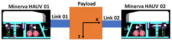
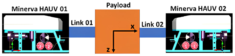
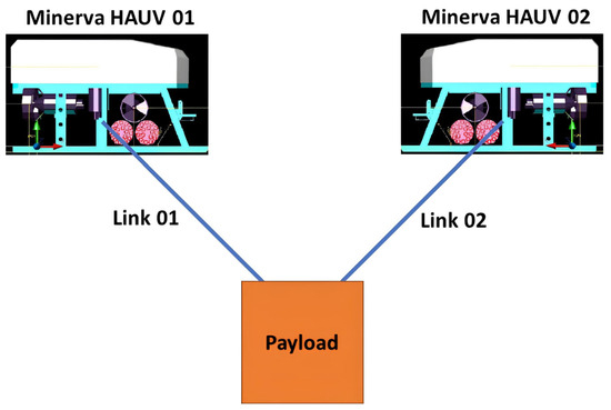
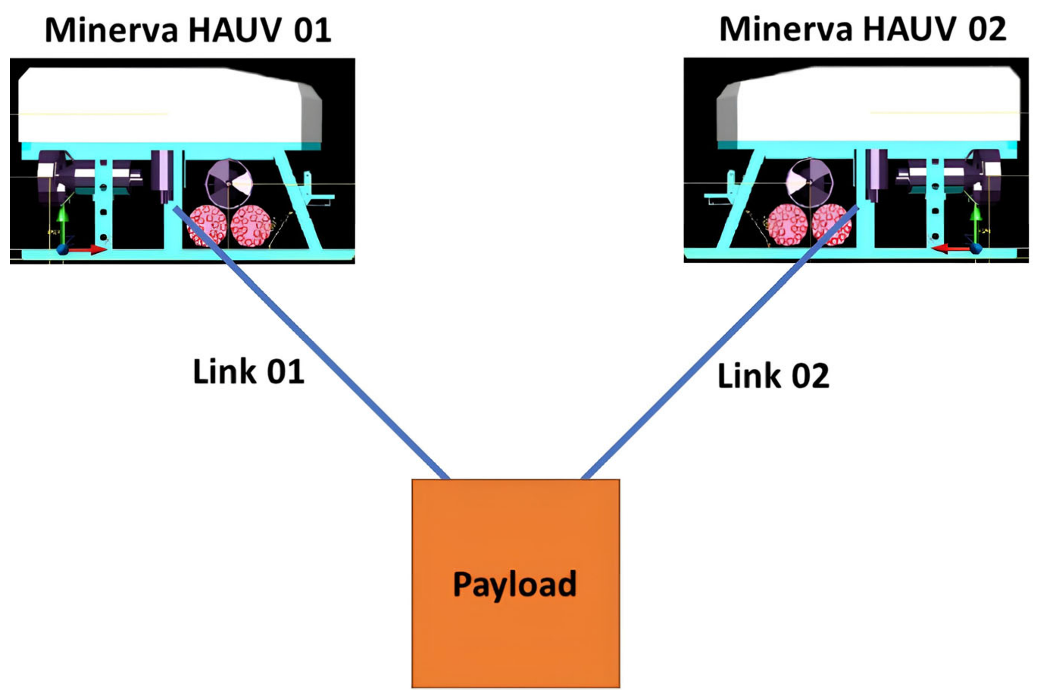
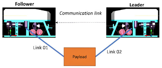
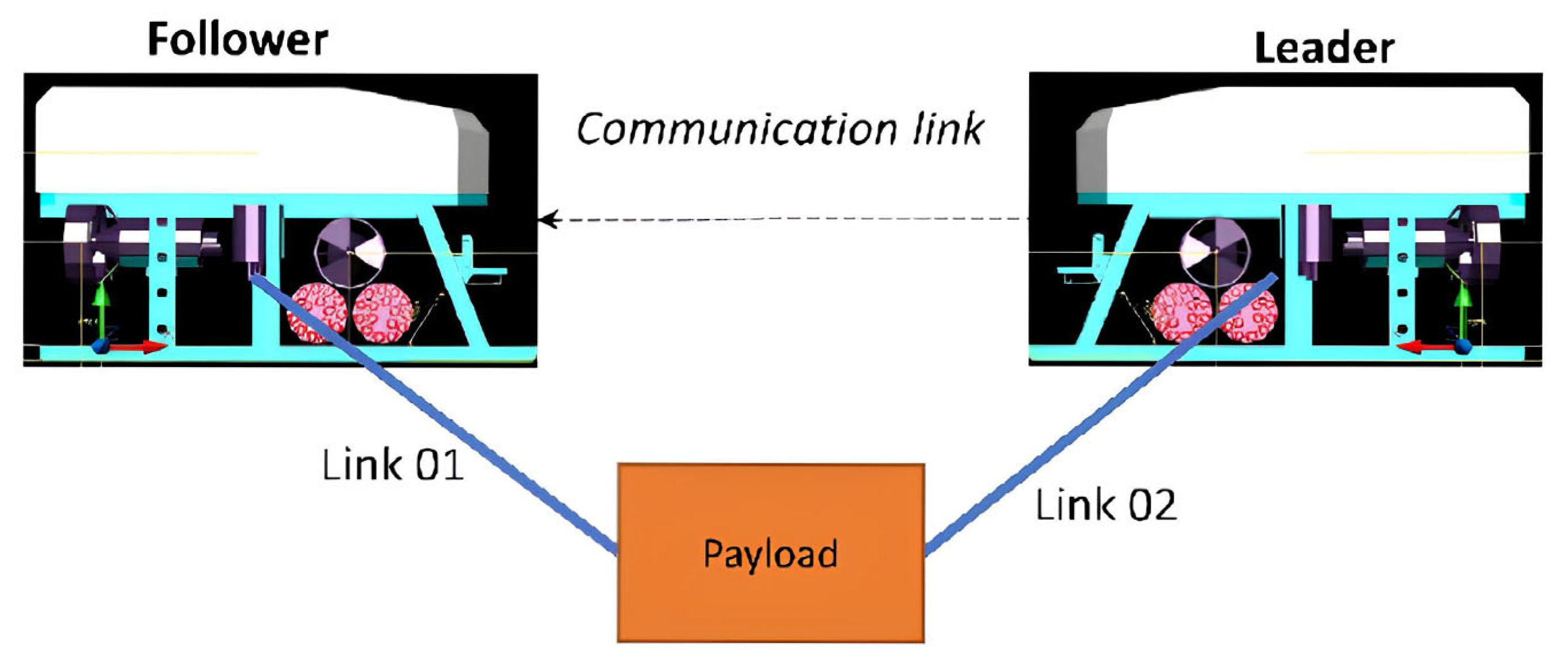
Three underwater-transportation configurations were developed, each involving a cubic payload transported by two Minerva HAUVs, as illustrated in Figure 1, Figure 2 and Figure 3. A two-vehicle arrangement was selected to enable detailed observation and analysis of the thrust actuation responses of each vehicle and its associated connection mechanism, whether through physical links or communication-based coordination, under different operational conditions. For the RCTS, rigid aluminum rods with dimensions of 1 m × 0.25 m × 0.01 m were used as connecting links between the vehicles and the payload. In the FCTS transportation configuration, the articulated links of 3 m in length were initially set to zero displacement angles. For the LFFCTS configuration, both the leader and follower HAUVs were initially positioned at zero pose. The follower vehicle was subsequently moved to the desired relative pose with respect to the leader through a formation controller.

Figure 1. Rigid-Connection Transportation System.

Figure 2. Flexible-Connection Transportation System.

Figure 3. Leader–Follower-Formation Control Transportation System.

A cubic container with a volume of 1 m³ is used to represent the payload, resulting in a buoyant force of approximately 10,055 N. In emergency situations, maintaining slightly positive buoyancy is desirable so that the payload can naturally ascend to the surface. For analytical simplicity, the payload in the RCTS configuration is assumed to be neutrally buoyant, corresponding to a mass of 1.025 kg. In contrast, for the FCTS configuration, maintaining neutral or slightly positive buoyancy is not practical. When the HAUVs attempt to move downward from an initial stationary state, the payload may remain stationary until sufficient tension develops in the articulated links, potentially causing collisions between the vehicles and leading to instability in the system [17]. To mitigate this issue, the payload weight is set slightly higher than its buoyancy, at 10,100 N (approximately 1030 kg).

For the LFFCTS configuration, the payload is also considered as negatively buoyant to ensure formation stability during transportation. Accordingly, the payload weight is maintained the same as that used in the FCTS transportation configuration.

3. Dynamic Model Development—Transportation Systems

For the development of a dynamic model for Autonomous Transportation Systems, the dynamic modeling of a single underwater vehicle has been studied in detail, as the fundamental principles governing underwater dynamics remain the same. The detailed derivation for single underwater vehicle is given in [1].

For the autonomous underwater transportation systems, a dynamic model for the RCTS is developed considering rigid connection between HAUVs and payload, whereas dynamic models for the FCTS and LFFCTS are developed considering flexible connections.

Studies conducted in a less complex single plane (vertical plane) enable effective verification of the responses under disturbances. They also enable effective investigation of controller and estimator countermeasures taken against the disturbances and noises. The following assumptions are made:

• The Coriolis and centripetal terms are discounted as the payload will be transported close to the area of operation using the support vessel;
• All the system components, i.e., the vehicles, payload, and links, are considered rigid bodies of constant masses with no force variation. The mass distribution throughout the transportation will remain the same;
• RCTS vehicles will have zero relative motion w.r.t. the payload;
• The transportation systems will be investigated below the base wave depth [18] to completely ignore surface wave effects;
• Interference with other underwater bodies is assumed to be negligible;
• The articulated joint links of the FCTS transportation configuration have negligible elasticity in this study;
• The FCTS links are also assumed to have zero mass as the values are less significant;
• The LFFCTS is also considered to have zero communication limitations, enabling a focus on the formation link between the leader and follower.

3.1. RCTS Development

Newton Euler formulation [19] is used for the development of a dynamic model for transportation configuration of the RCTS, similar to the method used for a single underwater vehicle. In this representation, the position as well as orientation of the transportation system is defined in an Earth-Fixed Frame (EFF), while velocities, forces and moments are defined in a Body-Fixed Frame (BFF). All moment calculations are referenced with respect to the center of the payload.

The equations of motion for the RCTS in matrix and vector form is shown in Equation (1), where ${\mathit{M}}_{\mathit{t}}$ is the mass matrix, as shown in Equation (2), ${\mathit{C}}_{\mathit{t}}\left(\mathit{v}\right)$ is the Coriolis and Centripetal matrix, ${\mathit{D}}_{\mathit{t}}\left(\mathit{v}\right)$ is the damping matrix, ${\mathit{g}}_{\mathit{t}}\left(\mathit{\eta }\right)$ is the matrix of complete hydrostatic terms, and ${\mathit{\tau }}_{\mathit{t}}$ is the thrust vector which includes the effects of all actuators in the RCTS.

$${\mathit{M}}_{\mathit{t}}\dot{\mathit{v}}+{\mathit{C}}_{\mathit{t}}\left(\mathit{v}\right)\mathit{v}+{\mathit{D}}_{\mathit{t}}\left(\mathit{v}\right)\mathit{v}+{\mathit{g}}_{\mathit{t}}\left(\mathit{\eta }\right)={\mathit{\tau }}_{\mathit{t}},$$

(1)

$${\mathit{M}}_{\mathit{t}}=\sum _{n=1}^k{(\mathit{M}}_{\mathit{h}\mathit{n}}+{\mathit{M}}_{\mathit{l}\mathit{n}})+{\mathit{M}}_{\mathit{p}}$$

(2)

The mass matrix for the nth HAUV among a cluster of k vehicles in the RCTS setup is denoted by ${\mathit{M}}_{\mathit{h}\mathit{n}}$. Analogously, ${\mathit{M}}_{\mathit{l}\mathit{n}}$ signifies the mass matrix for the nth link within the k link assembly, with ${\mathit{M}}_{\mathit{p}}$ identifying the mass of the transported payload.

The thrust-allocation matrix $\left({\mathit{T}}_{\mathit{a}\mathit{t}}\right)$ comprises the thrust effects of k HAUVs in the combined RCTS and is written as Equation (3), and the combined thrust force vector $\left({\mathit{f}}_{\mathit{t}}\right)$ for $j$ thrusters on $k$ HAUVs is expressed as shown in Equation (4). Finally, the combined thrust vector $\left({\mathit{\tau }}_{\mathit{t}}\right)$ is shown in Equation (5).

$${\mathit{T}}_{\mathit{a}\mathit{t}}=\left[{\mathit{T}}_{\mathit{a}1}{\mathit{T}}_{\mathit{a}2}\dots .{\mathit{T}}_{\mathit{a}\mathit{k}}\right],$$

(3)

$${\mathit{f}}_{\mathit{t}}={{[f}_1 f_2 f_3\dots \dots f_j]}^{\mathit{T}},$$

(4)

$${\mathit{\tau }}_{\mathit{t}}={\mathit{T}}_{\mathit{a}\mathit{t}}{\mathit{f}}_{\mathit{t}}$$

(5)

State terms will be reduced for the RCTS to only the vertical plane as we are analyzing the transportation systems only in the vertical plane. The kinematic part of the dynamic model becomes,

$$\dot{\mathit{\eta }}=\mathit{J}\mathit{v},$$

(6)

where the velocity vector of the underwater vehicle in the vertical plane in BFF ($\mathit{v})$, pose vector in EFF $\left(\mathit{\eta }\right)$ and transformation matrix ($\mathit{J}$) are shown in Equations (7), (8) and (9) respectively.

$$\mathit{v}=\left[\begin{array}{c}u\\ w\\ \begin{array}{c}\begin{array}{c}q\end{array}\end{array}\end{array}\right],$$

(7)

$$\mathit{\eta }=\left[\begin{array}{c}x\\ z\\ \begin{array}{c}\begin{array}{c}\theta \end{array}\end{array}\end{array}\right],$$

(8)

$$\mathit{J}=\left[\begin{array}{ccc}cos\theta & 0& -sin\theta \\ 0& 1& 0\\ sin\theta & 0& cos\theta \end{array}\right],$$

(9)

The complete state dynamics for the RCTS and a single vehicle of the LFFCTS in the vertical plane are written as,

$$\dot{\mathit{x}}=\left[\begin{array}{c}\dot{\mathit{\eta }}\\ \dot{\mathit{v}}\end{array}\right],$$

(10)

where $\dot{\mathit{\eta }}=\left[\begin{array}{c}\dot{x}\\ \dot{z}\\ \begin{array}{c}\begin{array}{c}\dot{\theta }\end{array}\end{array}\end{array}\right]$ and $\dot{\mathit{v}}=\left[\begin{array}{c}\dot{u}\\ \dot{w}\\ \begin{array}{c}\begin{array}{c}\dot{q}\end{array}\end{array}\end{array}\right]$.

3.2. FCTS Development

On the other hand, the Lagrangian approach [20] is used to derive the system dynamics of the FCTS transportation configuration. In this formulation, the payload center is selected as the reference point for deriving the governing equations. The relative motions of the vehicles with respect to the payload are taken in the EFF, and the moment components are evaluated about the payload center.

The Euler–Lagrange equation for the development of a dynamic model for the FCTS is given as [1]:

$${\displaystyle \frac{d}{dt}}\left({\displaystyle \frac{\mathsf{\partial }L}{\mathsf{\partial }{\dot{q}}_c}}\right)-{\displaystyle \frac{\mathsf{\partial }L}{\mathsf{\partial }{q}_c}}=Q_c,$$

(11)

where

$$L=T-U,$$

(12)

$T$ and $U$ are the sum of the kinetic and potential energies of all parts of the FCTS.

$q_c$ represents the coupled and interdependent coordinates, whereas $Q_c$ represents external forces and moments that are thrust forces and respective moments, in our case represented as ${\tau }_c$.

The motion dynamics in the vertical plane for the FCTS of multiple vehicles are written in matrix and vector form as given in Equation (13), where the Mass matrix ($\mathit{M}\left(\mathit{\eta }\right))$, Damping matrix ($\mathit{D}\left(\mathit{\eta },\dot{\mathit{\eta }}\right))$ and hydrostatic vector ($\mathit{g}\left(\mathit{\eta }\right))$ are given in Equations (14), (15) and (20) respectively.

$$\mathit{M}\left(\mathit{\eta }\right)\ddot{\mathit{\eta }}+\mathit{D}\left(\mathit{\eta },\dot{\mathit{\eta }}\right)\dot{\mathit{\eta }}+\mathit{g}\left(\mathit{\eta }\right)=\mathit{\tau },$$

(13)

$$\mathit{M}\left(\mathit{\eta }\right)=\left[\begin{array}{ccccccccc}{M}_t{+X}_{t\ddot{x}}& 0& 0& \cdots & 0& 0& -M_1{l}_{1}c{\alpha }_1& \cdots & {-M}_k{l}_{k}c{\alpha }_k\\ 0& M_t{+Z}_{t\ddot{z}}& 0& \cdots & 0& 0& M_1{l}_{1}s{\alpha }_1& \cdots & M_k{l}_{k}s{\alpha }_k\\ 0& 0& I_{y1}{+M_{\ddot{\theta }}}_1& \cdots & 0& 0& 0& \cdots & 0\\ ⋮& ⋮& ⋮& \ddots & ⋮& ⋮& ⋮& ⋮& ⋮\\ 0& 0& 0& \cdots & I_{yk}{+M_{\ddot{\theta }}}_k& 0& 0& \cdots & 0\\ 0& 0& 0& \cdots & 0& I_{yp}{+M_{\ddot{\theta }}}_p& 0& \cdots & 0\\ -M_1{l}_{1}c{\alpha }_1& M_1{l}_{1}s{\alpha }_1& 0& \cdots & 0& 0& M_1{l_1}^2& \cdots & 0\\ ⋮& ⋮& ⋮& \cdots & ⋮& ⋮& ⋮& \ddots & ⋮\\ -M_k{l}_{k}c{\alpha }_k& M_k{l}_{k}s{\alpha }_k& 0& \cdots & 0& 0& 0& \cdots & M_k{l_k}^2\end{array}\right],$$

(14)

$$\mathit{D}\left(\mathit{\eta },\dot{\mathit{\eta }}\right)=\left[\begin{array}{ccccccccc}{D}_{t_x}& 0& 0& \cdots & 0& 0& \begin{array}{c}{M}_1{l}_{1}s{\alpha }_1{\dot{\alpha }}_1\\ {-X_{\dot{x}}}_1{l}_{1}c{\alpha }_1\end{array}& \cdots & \begin{array}{c}{M}_k{l}_{k}s{\alpha }_k{\dot{\alpha }}_k\\ {-X_{\dot{x}}}_k{l}_{k}c{\alpha }_k\end{array}\\ 0& D_{t_z}& 0& \cdots & 0& 0& \begin{array}{c}{M}_1{l}_{1}c{\alpha }_1{\dot{\alpha }}_1\\ {+Z_{\dot{z}}}_1{l}_{1}s{\alpha }_1\end{array}& \cdots & \begin{array}{c}{M}_2{l}_{k}c{\alpha }_k{\dot{\alpha }}_k\\ {+Z_{\dot{z}}}_k{l}_{k}s{\alpha }_k\end{array}\\ 0& 0& {M_{\dot{\theta }}}_1& \cdots & 0& 0& 0& \cdots & 0\\ ⋮& ⋮& ⋮& \ddots & ⋮& ⋮& ⋮& ⋮& ⋮\\ 0& 0& 0& \cdots & {M_{\dot{\theta }}}_k& 0& 0& \cdots & 0\\ 0& 0& 0& \cdots & 0& {M_{\dot{\theta }}}_p& 0& \cdots & 0\\ {{-X}_{\dot{x}}}_1{l}_{1}c{\alpha }_1& {Z_{\dot{z}}}_1{l}_{1}s{\alpha }_1& 0& \cdots & 0& 0& D_{t_1}{l_1}^2& \cdots & 0\\ ⋮& ⋮& ⋮& \cdots & ⋮& ⋮& ⋮& \ddots & ⋮\\ {{-X}_{\dot{x}}}_k{l}_{k}c{\alpha }_k& {Z_{\dot{z}}}_k{l}_{k}s{\alpha }_k& 0& \cdots & 0& 0& 0& \cdots & D_{t_k}{l_k}^2\end{array}\right],$$

(15)

$X_{t\ddot{x}}$ and $Z_{t\ddot{z}}$ are the terms of added masses in surge and heave, respectively. Moreover, damping terms are shown in Equations (16)–(19).

$$D_{t_x}{=X_{\dot{x}}}_1+\dots {X_{\dot{x}}}_k+{X_{\dot{x}}}_p,$$

(16)

$$D_{t_z}{=Z_{\dot{z}}}_1+\dots {Z_{\dot{z}}}_k+{Z_{\dot{z}}}_p,$$

(17)

$$D_{t_1}={X_{\dot{x}}}_1+{Z_{\dot{z}}}_1,$$

(18)

$$D_{t_k}={X_{\dot{x}}}_k+{Z_{\dot{z}}}_k,$$

(19)

$$\mathit{g}\left(\mathit{\eta }\right)=\left[\begin{array}{c}0\\ g{M}_t-B_t\\ \left(z_{g_1}{W}_1-z_{b_1}{B}_1\right)\mathrm{s} {\theta }_1\\ ⋮\\ \left(z_{g_k}{W}_k-z_{b_k}{B}_k\right)\mathrm{s} {\theta }_k\\ -z_{b_p}{B}_p\mathrm{s}{\theta }_p\\ \left(W_1{-B}_1\right)l_{1}s{\alpha }_1\\ ⋮\\ \left(W_k{-B}_k\right)l_{k}s{\alpha }_k\end{array}\right],$$

(20)

The vector of the combined thrust forces and moments $\left(\mathit{\tau }\right)$ is given in Equation (21) and the vector of position, orientation and articulated links’ angles ($\mathit{\eta })$ is shown in Equation (22).

$$\mathit{\tau }=\left[\begin{array}{c}{\tau }_{x_p}\\ {\tau }_{z_p}\\ {\tau }_{\theta 1}\\ ⋮\\ {\tau }_{{\theta }_k}\\ {\tau }_{{\theta }_p}\\ {\tau }_{{\alpha }_1}\\ ⋮\\ {\tau }_{{\alpha }_k}\end{array}\right],$$

(21)

$$\mathit{\eta }=\left[\begin{array}{c}{x}_p\\ z_p\\ {\theta }_1\\ ⋮\\ {\theta }_k\\ {\theta }_p\\ {\alpha }_1\\ ⋮\\ {\alpha }_k\end{array}\right],$$

(22)

The position of each HAUV in the configuration of the FCTS in the vertical plane is written as Equation (23), where $k$ is the last HAUV of the system. The dynamics of the FCTS to obtain the states over time are shown in Equation (24).

$$\left[\begin{array}{c}{x}_n\\ z_n\end{array}\right]=\left[\begin{array}{c}{x}_p-l_{n}sin{\alpha }_n\\ z_p-l_{n}cos{\alpha }_n\end{array}\right] n=\mathrm{1,2},\dots ..k,$$

(23)

$$\dot{\mathit{x}}=\left[\begin{array}{c}\dot{\mathit{\eta }}\\ \ddot{\mathit{\eta }}\end{array}\right]=\left[\begin{array}{c}\mathit{v}\\ {\mathit{M}\left(\mathit{\eta }\right)}^{-1}(\mathit{\tau }-\mathit{D}\left(\mathit{\eta },\dot{\mathit{\eta }}\right)\dot{\mathit{\eta }}-\mathit{g}\left(\mathit{\eta }\right))\end{array}\right]$$

(24)

The actuator model is formulated based on the principle of virtual work, ensuring that the actuator’s positioning relative to the system’s center is accurately represented. The governing equation is expressed as:

$${\mathit{\tau }}_{\mathit{n}}={\sum }_{\mathit{ϵ}=1}^{\mathit{j}}{\sum }_{\mathit{n}=1}^{\mathit{k}}\mathit{n}{\displaystyle \frac{\mathit{\partial }\left({\mathit{f}}_{\mathit{ϵ}}.{\mathit{\xi }}_{\mathit{ϵ}}\right)}{\mathit{\partial }{\mathit{q}}_{\mathit{c}}}},$$

(25)

where $ϵ$ is the number of thrust actuators and $j$ is the last actuator in the system. $n$ is the number of HAUV $k$ is the last vehicle in the system. $f_{ϵ}$ is the actuation vector of each thrust actuator in the FCTS. ${\mathit{\xi }}_{ϵ}$ is the position of each actuator and is written as:

$${\mathit{\xi }}_{ϵ}={\mathit{\xi }}_{\mathit{Q}}+L_{Qϵ}{\mathit{e}}_{ϵ},$$

(26)

$L_{Qϵ}$ represents the distance of the actuator from the HAUV. ${\mathit{e}}_{ϵ}$ the directional vector for $L_{Qϵ}$. ${\mathit{\xi }}_{\mathit{Q}}$ shows the position of the HAUV w.r.t the payload, written as

$${\mathit{\xi }}_{\mathit{Q}}={\mathit{\xi }}_{\mathit{p}}+l\mathit{\rho }$$

(27)

${\mathit{\xi }}_{\mathit{p}}$ shows the position of the payload, $l$ is the length of an articulated link and $\mathit{\rho }$ is the unit vector in the direction of $l$.

In the FCTS, the vehicles must maintain the prescribed inter-vehicle spacing, while tracking the desired trajectory, and simultaneously maintain the required articulation angles of the connecting links.

3.3. LFFCTS Development

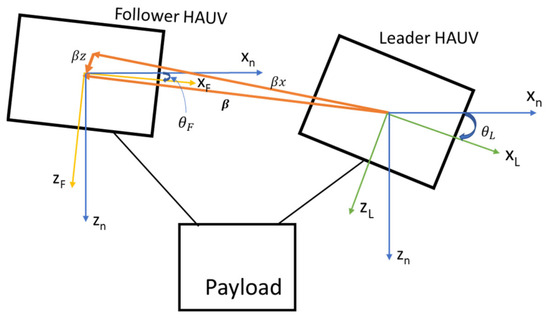
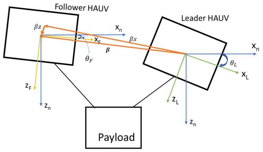
The dynamic model for each vehicle of the LLFCTS remains the same as given in [1]. Figure 4 illustrates the absolute and relative poses of the leader and follower HAUVs. The separation between the vehicles is defined by the components $x_L-x_F$ and $z_L-z_F$, where the subscripts $L$ and F denote the leader and follower, respectively. To calculate the follower’s relative displacement from the leader, these coordinates are mapped into the leader’s BFF as follows:

$$\left[\begin{array}{c}{\beta }_x\\ {\beta }_z\end{array}\right]=\left[\begin{array}{cc}-cos{\theta }_L& -sin{\theta }_L\\ sin{\theta }_L& -cos{\theta }_L\end{array}\right]\left[\begin{array}{c}{x}_L-x_F\\ z_L-z_F\end{array}\right],$$

(28)

Or

$${\beta }_x=-\left(x_L-x_F\right)cos{\theta }_L-\left(z_L-z_F\right)sin{\theta }_L,$$

(29)

$${\beta }_z=\left(x_L-x_F\right)sin{\theta }_L-\left(z_L-z_F\right)cos{\theta }_L,$$

(30)

Figure 4. Pose of leader and follower of LFFCTS.

By differentiating Equations (29) and (30) in conjunction with kinematic models for both vehicles, the time derivatives for the leader and follower separation are obtained. The overall formation dynamics are then established by integrating these varying distance components with the relative angular orientation, as formulated in Equations (31)–(33).

$${\dot{\beta }}_x={-u}_L{+u}_{F}cos{\theta }_{LF}{+w}_{F}sin{\theta }_{LF}+{{\beta }_{z}r}_L,$$

(31)

$${\dot{\beta }}_z={-w}_L{-u}_{F}sin{\theta }_{LF}+w_{F}cos{\theta }_{LF}-{{\beta }_{x}r}_L,$$

(32)

$${\dot{\theta }}_{LF}=r_L-r_F,$$

(33)

where $(u_L, w_L)$ and $(u_F, w_F)$ are the velocity terms in the translational direction for the leader and follower vehicles respectively, and $r_L$ and $r_F$ are the angular velocities of these vehicles respectively. ${\theta }_{LF}$ is the difference between the pitch angles of the leader and follower, as given in Equation (34):

$${\theta }_{LF}={\theta }_L-{\theta }_F,$$

(34)

Putting Equations (31)–(33) into matrix form produces:

$$\dot{\mathit{\chi }}=\mathit{F}\left(\mathit{\chi }\right)+\mathit{G}\left(\mathit{\chi }\right){\mathit{v}}_{\mathit{F}},$$

(35)

where

$$\mathit{\chi }=[{\beta }_x {\beta }_z {\theta }_{LF}{]}^T,$$

(36)

$${\mathit{v}}_{\mathit{F}}=[u_F w_F r_F{]}^T,$$

(37)

$$\mathit{F}\left(\mathit{\chi }\right)=\left[\begin{array}{c}{\beta }_z{r}_L-u_L\\ {-\beta }_x{r}_L{-w}_L\\ r_L\end{array}\right],$$

(38)

$$\mathit{G}\left(\mathit{\chi }\right)=\left[\begin{array}{ccc}cos{\theta }_{LF}& sin{\theta }_{LF}& 0\\ -sin{\theta }_{LF}& cos{\theta }_{LF}& 0\\ 0& 0& -1\end{array}\right],$$

(39)

By applying the technique of dynamic inversion, the actuation control input may be formulated as:

$${\mathit{v}}_{\mathit{F}}={\mathit{G}}^{-1}\left(\mathit{\chi }\right)\left(-\mathit{F}\left(\mathit{\chi }\right)+\dot{\mathit{\chi }}\right),$$

(40)

When a linear-feedback control law is employed as the formation controller, the resulting expression is as follows:

$$\dot{\mathit{\chi }}=-{\mathit{k}}_{\mathit{f}}\left(\mathit{\chi }-{\mathit{\chi }}_{\mathit{d}}\right)$$

(41)

Consequently, the formation controller gain matrix $\left({\mathit{k}}_{\mathit{f}}\right)$ ensures that the distance errors between the leader and follower $(e_{\beta x},e_{\beta z})$, along with the relative pitch angle error $\left(e_{\theta }\right)$, asymptotically converge to zero.

3.4. Parameters of Transportation Systems

As discussed before, system parameters for the transportation systems are adopted from the Minerva HAUV model [16], while link and payload parameters are derived from DNV-GL data. Actuation input to obtain the desired states varies depending on the transportation configuration: for the RCTS, only translational motion states are considered; for the FCTS, the link displacement angles are included alongside translational states; and for the LFFCTS, the translational motion states of each vehicle are treated independently.

4. Estimator Design

Underwater vehicles can be subjected to sea currents [21,22,23], sea waves [24,25], and interactions with the sea bed [26], other underwater vehicles, sea animals or underwater structures [27,28,29]. The effect of sea waves is ignored in this research due to the assumption of deep-water operation. On the other hand, sea currents and interaction effects, as mentioned above, could be applied under constant or random variation states [30,31,32]. In this research, the effects due to random variation in these factors are taken as process noise.

Navigation sensors are required to locate an underwater vehicle. Noise can be added due to the limitations of the equipment, for example, during amplification by amplifiers and Analog-to-Digital Conversion by ADCs. There are environmental factors that could add noise to the sensors. The sensor signals are affected by noise, resulting in inaccuracies/fluctuations that require rectification.

The Kalman Filter (KF) is employed to estimate the complete state of the vehicle in the presence of stochastic disturbances and measurement noise. It is an optimal recursive estimator that combines system model predictions with sensor observations to minimize the effects of process and measurement uncertainties, thereby providing an accurate estimate of the system state for actuators to use [33,34,35,36].

The Nonlinear Extended Kalman Filter [37] is used for the nonlinear system in this research due to its accurate estimation and is widely used for unmanned underwater vehicles [38,39].

The EKF is written as shown in Equation (42) assuming that both process noise $\left({\mathit{w}}_{\mathit{d}}\right)$ and sensor noise $\left({\mathit{w}}_{\mathit{n}}\right)$ are zero-mean white Gaussian processes.

$$\mathbb{E}\left({\mathit{w}}_{\mathit{d}}\left(t\right){\mathit{w}}_{\mathit{d}}{\left(\zeta \right)}^{\mathit{T}}\right)={\mathit{V}}_{\mathit{d}}∆\left(\mathit{t},\zeta \right),$$

(42)

$$\mathbb{E}\left({\mathit{w}}_{\mathit{d}}\left(t\right){\mathit{w}}_{\mathit{n}}{\left(\zeta \right)}^{\mathit{T}}\right)=0,$$

(43)

$$\mathbb{E}\left({\mathit{w}}_{\mathit{n}}\left(t\right){\mathit{w}}_{\mathit{n}}{\left(\zeta \right)}^{\mathit{T}}\right)={\mathit{V}}_{\mathit{n}}∆\left(\mathit{t},\zeta \right),$$

(44)

where

$$∆\left(t,\zeta \right)=\{\begin{array}{c}1 if t=\zeta \\ 0 if t\ne \zeta \end{array}\}$$

(45)

$\mathbb{E}$ denotes the expected value (probabilistic mean) of a random variable, as detailed by Michel Dekking [40]. ${\mathit{V}}_{\mathit{d}}$ and ${\mathit{V}}_{\mathit{n}}$ are positive semi-definite variance matrices, representing sensor and process noise, respectively.

The EKF estimates system states in two stages: prediction and update, yielding optimal state estimates for the underwater vehicle [41].

The nonlinear dynamics of an HAUV are expressed as:

$$\dot{\mathit{x}}=\mathit{f}\left(\mathit{x},\mathit{\tau }\right)+{\mathit{w}}_{\mathit{d}},$$

(46)

$\mathit{x}$ is the state vector and $\mathit{\tau }$ is the actuator control input.

The measurement vector $\mathit{z}$ can be written as:

$$\mathit{z}=\mathrm{h}\left(\mathit{x}\right)+{\mathit{w}}_{\mathit{n}},$$

(47)

$h\left(x\right)$ represents the measured state values influenced only by process noise, whereas $z$ reflects the combined effect of both sensor and process noises. The estimated state vector at the next time-step ${{(x}_k}^{-})$ is achieved by integrating the vehicle dynamics based on the previous time-step state vector ${(\widehat{x}}_{k-1}).$ The corresponding predicted error covariance matrix $\left({P_k}^{-}\right)$ is written as Equation (48).

$${{\mathit{P}}_{\mathit{k}}}^{-}={\mathit{F}}_{\mathit{k}}{\widehat{\mathit{P}}}_{\mathit{k}-1}{{\mathit{F}}_{\mathit{k}}}^{\mathit{T}}+{\mathit{V}}_{\mathit{d}},$$

(48)

$F_k$ represents the Jacobian matrix of states, as given in Equation (49), and the Kalman Filter gain matrix $\left({\mathit{K}}_{\mathit{k}}\right)$ is determined as shown in Equation (50).

$${\mathit{F}}_{\mathit{k}}={{\displaystyle \frac{\mathsf{\partial }f({\mathit{x}}_{\mathit{k}},{\mathit{\tau }}_{\mathit{k}})}{\mathsf{\partial }{\mathit{x}}_{\mathit{k}}}}|}_{{\mathit{x}}_{\mathit{k}}={\widehat{\mathit{x}}}_{\mathit{k}-1}},$$

(49)

$${\mathit{K}}_{\mathit{k}}={{\mathit{P}}_{\mathit{k}}}^{-}{{\mathit{H}}_{\mathit{k}}}^{\mathit{T}}[{\mathit{H}}_{\mathit{k}}{{\mathit{P}}_{\mathit{k}}}^{-}{{\mathit{H}}_{\mathit{k}}}^{\mathit{T}}+{\mathit{V}}_{\mathit{n}}{]}^{-1},$$

(50)

${\mathit{H}}_{\mathit{k}}$ is the Jacobian matrix of measurements, written as Equation (51), and the state vector in the next step $\left({\widehat{\mathit{x}}}_{\mathit{k}}\right)$ can be determined as shown in Equation (52).

$${\mathit{H}}_{\mathit{k}}={{\displaystyle \frac{\mathsf{\partial }\mathit{h}\left(\mathit{x}\right)}{\mathsf{\partial }\mathit{x}}}|}_{\mathit{x}={{\mathit{x}}_{\mathit{k}}}^{-}},$$

(51)

$${\widehat{\mathit{x}}}_{\mathit{k}}={{\mathit{x}}_{\mathit{k}}}^{-}+{\mathit{K}}_{\mathit{k}}\left[{\mathit{z}}_{\mathit{k}}-{{\mathit{h}(\mathit{x}}_{\mathit{k}}}^{-})\right],$$

(52)

Finally, the updated Error Variance Matrix $\left({\widehat{\mathit{P}}}_{\mathit{k}}\right)$ is written as:

$${\widehat{\mathit{P}}}_{\mathit{k}}=\left[\mathit{I}-{\mathit{K}}_{\mathit{k}}{\mathit{H}}_{\mathit{k}}\right]{{\mathit{P}}_{\mathit{k}}}^{-}[\mathit{I}-{\mathit{K}}_{\mathit{k}}{\mathit{H}}_{\mathit{k}}{]}^{\mathit{T}}+{\mathit{K}}_{\mathit{k}}{\mathit{V}}_{\mathit{n}}{{\mathit{K}}_{\mathit{k}}}^{\mathit{T}}$$

(53)

5. Actuation Control Architecture

The control system is applied on the thrust actuators of the transportation systems to track the desired trajectory. For obtaining the desired trajectory, a minimum snap trajectory tool is used [7,42].

A centralized actuation control architecture is implemented for both the RCTS and FCTS, as illustrated in Figure 5. In this framework, the controller operates on the error $\left(e\right)$, defined as the difference between the desired $\left(x_d\right)$ and measured $\left(x\right)$ state vectors. For the RCTS configuration, the control state vector includes the vehicle position, yaw angle, and the corresponding velocity components. Roll and pitch dynamics are excluded from the actuation control design because hydrostatic restoring moments naturally return the system to an upright orientation. In contrast, the FCTS configuration incorporates the articulated links’ angles in addition to the payload position and yaw angle in actuation control. Consequently, the dimension of the state vector depends on the number of articulated links, which in turn is determined by the number of HAUVs participating in the cooperative system.

Figure 5. Actuation control of RCTS and FCTS.

The controller output is generated as a thrust actuation vector in the EFF $\left({\tau }_e\right)$. In the case of the FCTS, this vector directly represents the desired thrust. For the RCTS, however, it is transformed into the BFF by multiplying it with the inverse of the transformation matrix $\left(J^{-1}\right)$, producing the desired thrust actuation vector $\left({\tau }_d\right)$. The desired thrust is subsequently mapped to the individual actuation units by applying the inverse of the thrust-allocation matrix $\left({T_a}^{-1}\right)$, yielding the desired thrust force vector for actuation $f_d$. A saturation function is applied to obtain the realizable thrust force vector $\left(f\right)$, which is then processed by the thrust actuation model to generate the actual thrust actuation vector ($\tau )$. This thrust is applied as the control input to the system’s dynamic model to obtain the updated state vector $\left(x\right)$. The resulting state is continuously compared with the desired state $\left(x_d\right)$ to compute the error, and the process iterates until the required system response is achieved.

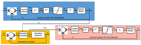
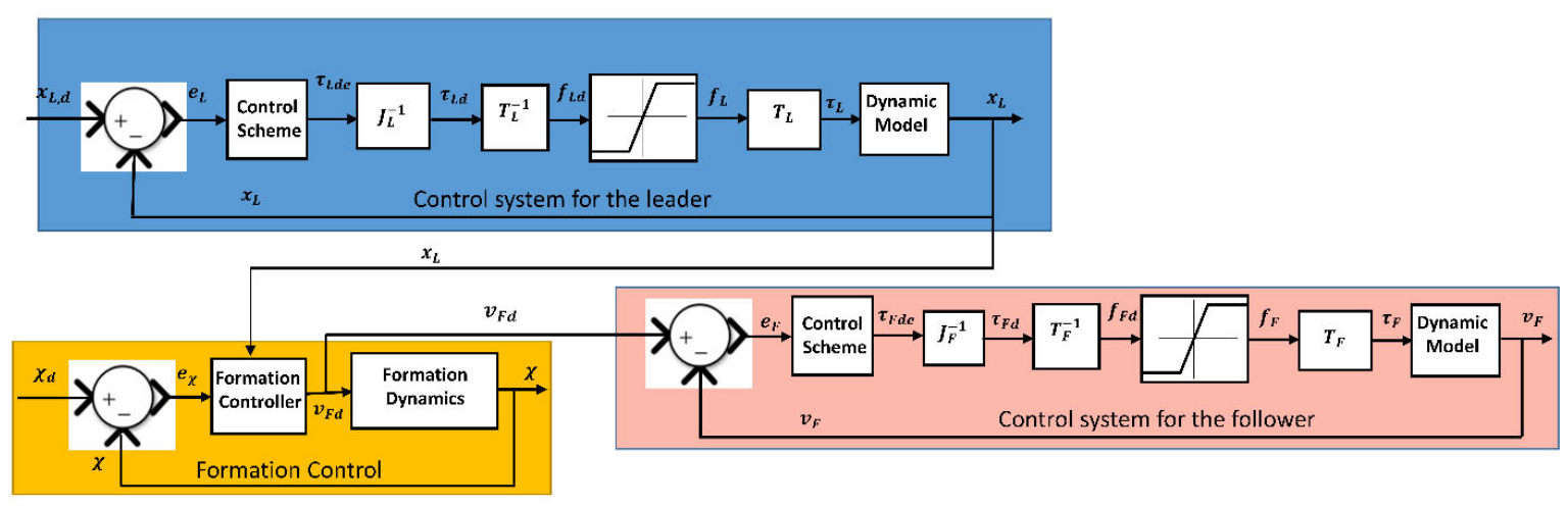
A distributed actuation control architecture is implemented for the LFFCTS configuration, as illustrated in Figure 6. In this approach, a control system is first applied to the leader vehicle to generate its desired state vector $\left(x_{Ld}\right)$. The measured states of the leader HAUV $\left(x_L\right)$ are then transmitted to the formation control module while also serving as feedback for the leader’s control loop. The formation controller operates on the error $\left(e_{\chi }\right)$, defined as the difference between the desired $\left({\chi }_d\right)$ and the current parameters $\left(\chi \right)$ of the formation.

Figure 6. Actuation control of LFFCTS.

Based on this error and the leader’s actual states, the formation controller provides an input command to the actuators to obtained the desired velocity vector for the follower $\left(u_{Fd}\right)$. This desired velocity vector is compared with the measured follower velocity vector $\left(u_F\right)$ to determine the error $\left(e_F\right)$. The follower control system then acts on this error signal to regulate the follower’s motion through actuators, enabling it to achieve the desired response relative to the leader while maintaining the specified formation.

6. Neural Network-Augmented Controller (NNAC)

Artificial Neural Networks (ANNs) are a recent development towards making complex calculations and fitting nonlinear functions as simply as possible. ANNs are very efficient if they are trained with sufficient input–output data, they can even forecast output values for input values not in the training input range. ANNs’ capabilities of prediction and estimation are mainly due to the alteration of their intrinsic parameters in order to emulate the input–output relationships for which the ANNs are trained. Neural Networks have been employed in marine applications along with many other fields of research [43,44,45,46]. In [47], ANNs are applied to predict the results of towing tank tests and interpolated data used in these tests.

PID controllers are the most used controllers in industries due to their simpler structure and pragmatic design. However, PID-based controllers have a few limitations and lack adaptiveness. Controlled plants have varying parameters, and these simple controllers could hardly adapt to the change in plants due to both internal and external disturbances. Many advanced control techniques have been employed by researchers in the past to tackle problems concerning the adaptivity of the controllers. In [48], the Model Reference Adaptive Controller is used with an appropriate reference model and PD controller to ensure the dynamic positioning of sea-going vessels. This method has a clear disadvantage in terms of employing a suitable reference model and appropriate scheduling of gains. Similarly, in [49], an adaptive controller in terms of a fuzzy rule-based PID controller is employed for the control of semi-submersible marine platforms. This type of controller has better adaptability to changes in environment but also requires large amplitudes for the control force, which in turn requires an enhanced requirement for mechanical systems with respect to thrusters. In [50], Adaptive Neuro-Fuzzy Inference Systems (ANFISs) are applied for the control of robotic arms integrated into the battery-switching mechanism for a collaborative network of mobile robots.

Neural Network-based control allocation approaches were employed for dynamic positioning (DP) of ships in recent studies. In [51], an Extreme Learning Machine (ELM)-based Neural Network thruster allocation scheme was employed that used thruster force and command measurements for the training of the network and provision of control allocation for the test data. A typical PID motion controller was used in this research along with a Neural Network-based allocation method. A suitable architecture and number of neurons in the hidden layer for shallow Neural Networks were selected based on the optimized performance. The proximal Policy Optimization algorithm was used in [52] to implement a Deep Reinforcement Learning (DRL) control scheme for DP problems. The results obtained in both the simulations and sea trials were excellent. A pre-trained neural DRL-based controller was less time-consuming in online operations; however, a certain amount of time was required to train and test the DRL before it could be employed in the real scenario. To address the complexities of environmental disturbances during this process, an ESO-enhanced actor–critic reinforcement learning approach was adapted in [53], where an observer compensates for lumped uncertainties to streamline the learning of tracking controls for marine vessels. Furthermore, for systems involving multiple vehicles where communication overhead is a concern, a fixed-time event-triggered consensus protocol was developed in [54] to maintain high-precision coordination while significantly reducing unnecessary actuation and data transmission.

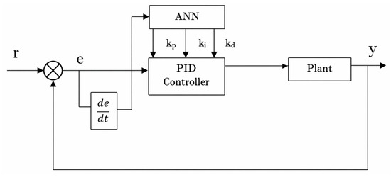
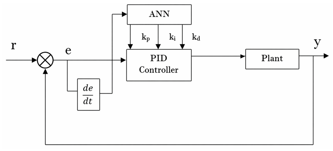
To enhance self-adaptability, Neural Networks can be applied to realize the real-time adjustment of controller parameters. A combination of the learning characteristics of Artificial Neural Networks (ANNs) with PID control presents a robust solution. The structure of the PID controller based on a Back Propagation (BP) Neural Network is shown in Figure 7. The architecture comprises a PID controller for closed-loop stability and a Back Propagation (BP) Neural Network that dynamically modifies weight coefficients to tune the PID parameters (Kp, Ki, Kd). By tuning the PID parameters through the Neural Network, a certain performance objective can be optimized.

Figure 7. NN-based PID controller—block diagram.

The BP Neural network uses both forward and reverse transmission to minimize the output error signal. Reverse transmission alters the weights of neurons based on the output error. Rather than relying on static gains, the ANN continuously monitors the state of the system by taking the tracking error ($e$) and its derivative ($\dot{e}$) as primary inputs. This allows the network to capture the complex, nonlinear dynamics and environmental disturbances inherent in underwater operations. Based on these real-time inputs, the ANN dynamically computes and updates the proportional (Kp), integral (Ki) and derivative (Kd) gains. These updated gains are then supplied to the PID controller, where the proportional, integral, and derivative actions are internally realized in a standard manner. The auto-tuning capability of NNAC ensures the PID controller remains optimized for varying conditions, directly contributing to the significant RMSE reductions observed in this study and providing a level of precision that conventional fixed-gain controllers cannot achieve.

7. Controller Implementation

The states of the RCTS and FCTS are centrally controlled using PID control. On the other hand, individual vehicles of the LFFCTS are separately controlled using PID control, and the formation controller of the LFFCTS is used as a linear feedback state controller with a gain value of 1.5.

7.1. Neural Network-Augmented Control (NNAC)

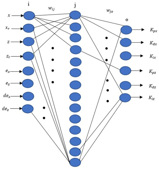
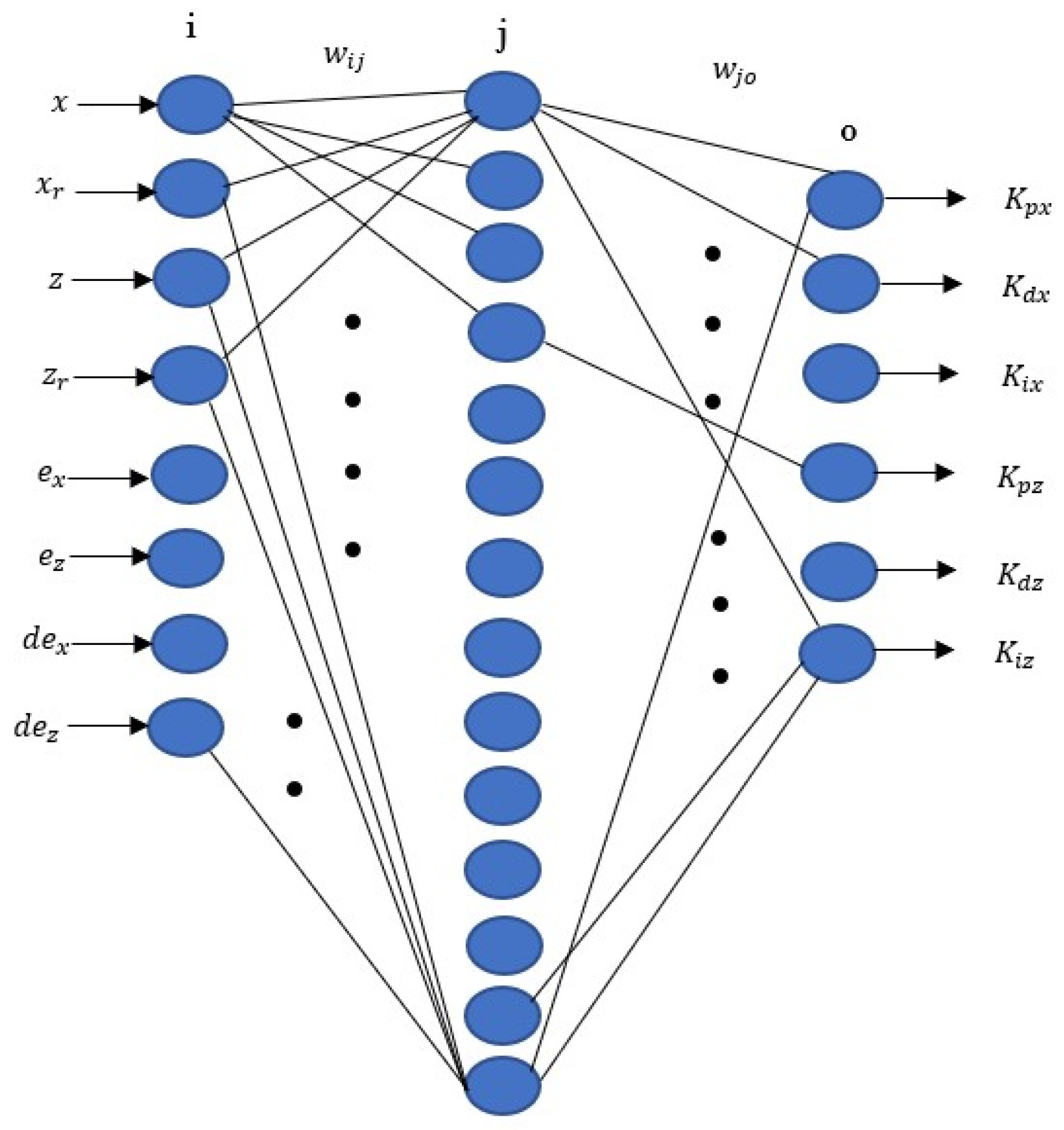
In this paper, a Neural Network (NN) is applied to tune the parameters of PID controllers to achieve the desired motion response of the transportation systems. The actual states, desired states, and errors between the actual and desired states, as well as error derivatives, are used as nodes in the input layer. A hidden layer is employed to provide the most optimized outcomes after trials. The weights of the connection between input and hidden layers are represented as $w_{ij}$. The output layer contains the parameters of PID controllers for the states which are required to be controlled by minimizing the performance index function as

$$\mathbf{E}(\mathbf{k})={\displaystyle \frac{1}{2}}(\mathbf{r}(\mathbf{k})-\mathbf{y}(\mathbf{k}){)}^2,$$

(54)

At each sampling instant, the NN receives the current system error signals, computes updated PID gains, and supplies them to the controller. The resulting control action affects the plant output, which in turn updates the error signal. This closed-loop interaction enables the NN to continuously learn the relationship between system dynamics and optimal controller parameters.

These parameters are optimized for the changes in the state readings of the transportation systems. The weights of the connection between hidden and output layers are represented by $w_{jo}$. The weights between input/ hidden layers and hidden/output layers get updated by employing the gradient descent method to obtain the optimized control parameters for the states of the transportation systems. It works by following the negative gradient direction of E(k) for weights to optimize and attaching an inertia item for faster convergence to the global minimum.

$$\mathsf{\Delta }{\mathsf{\omega }}_{\mathbf{i}\mathbf{l}}^{\left(3\right)}\left(\mathbf{k}\right)=-\mathsf{\eta }{\displaystyle \frac{\mathsf{\partial }\mathbf{E}\left(\mathbf{k}\right)}{\mathsf{\partial }{\mathsf{\omega }}_{\mathbf{i}\mathbf{l}}^{\left(3\right)}}}+\mathsf{\alpha }\mathsf{\Delta }{\mathsf{\omega }}_{\mathbf{i}\mathbf{l}}^{\left(3\right)}\left(\mathbf{k}-1\right),$$

(55)

$\mathsf{\eta }$ is the learning rate and $\mathsf{\alpha }$ is the momentum factor.

$${\displaystyle \frac{\mathsf{\partial }\mathit{E}\left(\mathit{K}\right)}{\mathsf{\partial }{\mathit{\omega }}_{\mathit{i}\mathit{l}}^{\left(3\right)}\left(\mathit{k}\right)}}={\displaystyle \frac{\mathsf{\partial }\mathit{E}\left(\mathit{k}\right)}{\mathsf{\partial }\mathit{y}\left(\mathit{k}\right)}}·{\displaystyle \frac{\mathsf{\partial }\mathit{y}\left(\mathit{k}\right)}{\mathsf{\partial }\mathit{u}\left(\mathit{k}\right)}}·{\displaystyle \frac{\mathsf{\partial }\mathit{u}\left(\mathit{k}\right)}{\mathsf{\partial }{\mathit{o}}_{\mathit{i}}^{\left(3\right)}}}·{\displaystyle \frac{\mathsf{\partial }{\mathit{o}}_{\mathit{i}}^{\left(3\right)}}{\mathsf{\partial }\mathit{n}\mathit{e}{\mathit{t}}_{\mathit{i}}^{\left(3\right)}}}·{\displaystyle \frac{\mathsf{\partial }\mathit{n}\mathit{e}{\mathit{t}}_{\mathit{i}}^{\left(3\right)}\left(\mathit{k}\right)}{\mathsf{\partial }{\mathit{\omega }}_{\mathit{i}\mathit{l}}^{\left(3\right)}\left(\mathit{k}\right)}},$$

(56)

$\mathbf{u}\left(\mathbf{k}\right)$ is the output of the controller at instant k and ${\mathbf{o}}_{\mathbf{i}}^{\left(3\right)}$ is the output of all nodes in the output layer, given as ${\mathbf{o}}_1^{\left(3\right)}={\mathbf{k}}_{\mathbf{p},}{\mathbf{o}}_2^{\left(3\right)}={\mathbf{k}}_{\mathbf{i}},{\mathbf{o}}_3^{\left(3\right)}={\mathbf{k}}_{\mathbf{d}}$, whereas $\mathbf{n}\mathbf{e}{\mathbf{t}}_{\mathbf{i}}^{\left(3\right)}$ is the input of all nodes in the output layer.

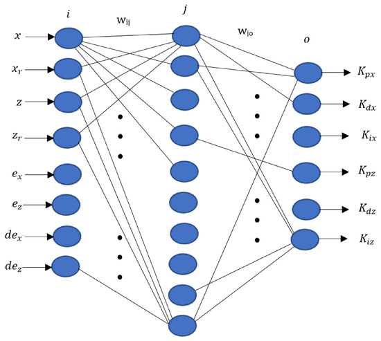
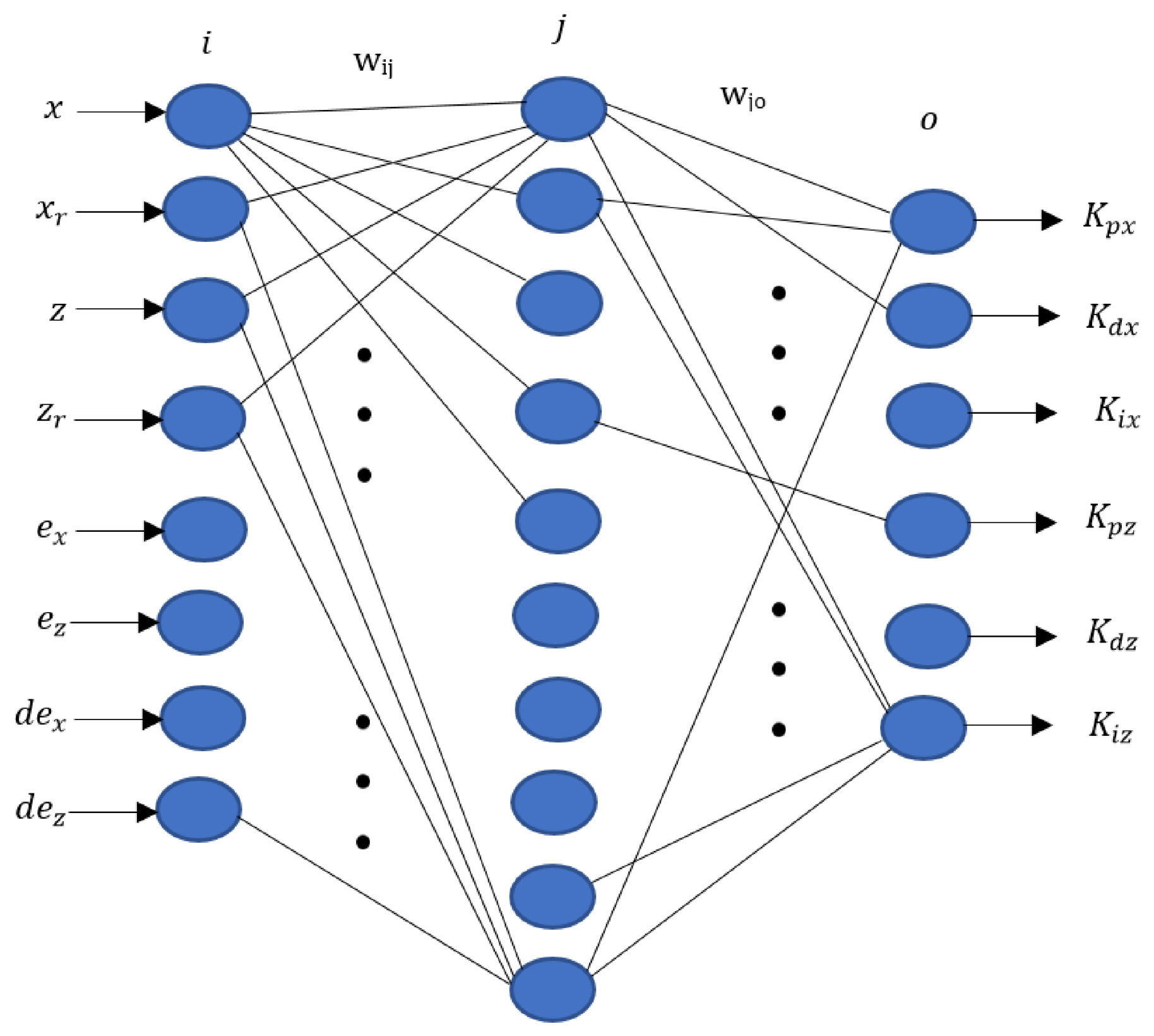
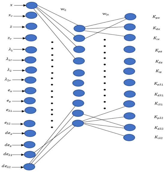
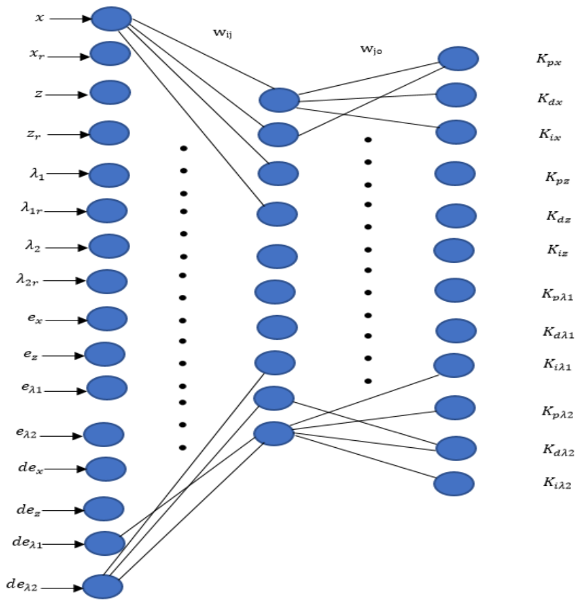
The Neural Network for the RCTS has an 8-14-6 structure, as shown in Figure 8. For each vehicle of the LFFCTS, the NN has an 8-10-6 structure, as shown in Figure 9. Although both the RCTS and a single vehicle of the LFFCTS are modeled using rigid-body dynamics, the Neural Network architecture for the RCTS employs 14 hidden neurons, whereas the single LFFCTS vehicle uses only 10 hidden neurons. This difference arises because the rigidly connected RCTS configuration comprises two HAUVs, two manipulators and a payload, forming a comparatively larger and more complex rigid structure than a single HAUV. Consequently, achieving and maintaining the pitch angle response of the RCTS within ±2 degrees demands greater control efforts. Moreover, the Neural Network for the FCTS, as illustrated in Figure 10, adopts a 16–10–12 architecture, as the vehicles must independently maintain their positions and orientations with respect to the payload. The output layer uses the non-negative sigmoid function as the activation function while the hidden layer uses the negative and positive symmetric sigmoid functions. The output layer employs a non-negative sigmoid function, as the output cannot be negative.

Figure 8. NN architecture—RCTS.

Figure 9. NN architecture—each vehicle of LFFCTS.

Figure 10. NN architecture—FCTS.

$x$ and $z$ are the actual states in surge and heave. $x_r$ and $z_r$ are the desired states in surge and heave. $e_x$ and $e_z$ are the differences between the actual and desired states in surge and heave, respectively. $d{e}_x$ and ${de}_z$ are the error differentials in the direction of surge and heave, respectively.${\lambda }_1$ and ${\lambda }_2$ are the actual articulated link angles of the FCTS. ${\lambda }_{1r}$ and ${\lambda }_{2r}$ are the desired articulated link angles of the FCTS. $e_{\lambda 1}$ and $e_{\lambda 2}$ are the differences between the actual and desired articulated link angles. ${de}_{\lambda 1}$ and $d{e}_{\lambda 2}$ are the differential of the errors in the displacement angles.

After several simulation tests with various NN parameters, the selected parameters for the transportation systems are shown in Table 1.

Table 1. BPNN parameters.

S. No.	Parameters	RCTS	FCTS	LFFCTS
1.	Learning rate $\left(\eta \right)$	0.5	0.5	0.5
2.	Momentum factor	0.1	0.1	0.1
3.	Gain adjustment	20 (surge) 18 (heave)	20 (surge) 30 (heave) 500 (displacement angle link 01) 500 (displacement angle link 02)	18 (leader’s surge) 15 (leader’s heave) 4 (follower’s surge) 4 (follower’s heave)

7.2. Conventional PID Control

For comparison purposes, a conventional PID controller with manual tuning of PID gains is also implemented on the autonomous transportation systems under sensor and process noise. In this regard, several simulation tests were performed using different PID gains. After confirming the reasonable trajectory tracking at several simulation runs, the PID gains are selected as mentioned in Table 2, Table 3 and Table 4 for the RCTS, FCTS and LFFCTS respectively.

Table 2. PID gains for RCTS.

	${\mathit{K}}_{\mathit{P}}$	${\mathit{K}}_{\mathit{I}}$	${\mathit{K}}_{\mathit{D}}$
Surge	100	0.5	5
Heave	100	0.5	5
Pitch	10	1	2

Table 3. PID gains for FCTS.

	${\mathit{K}}_{\mathit{P}}$	${\mathit{K}}_{\mathit{I}}$	${\mathit{K}}_{\mathit{D}}$
Surge	100	0.1	5
Heave	100	0.5	5
Pitch	10	1	2
Swing angle 01	1000	10	50
Swing angle 02	800	10	40

Table 4. PID gains for LFFCTS.

		${\mathit{K}}_{\mathit{P}}$	${\mathit{K}}_{\mathit{I}}$	${\mathit{K}}_{\mathit{D}}$
Leader	Surge	70	0.2	3
	Heave	100	0.5	3
	Pitch	10	2	1
Follower	Surge	15	3	1
	Heave	15	6	1
	Pitch	10	2	1

8. Planned Trajectory

Due to their centralized actuation control architecture, both the RCTS and FCTS were assigned the task of following a predefined trajectory as an integrated system. In contrast, within the LFFCTS configuration, the leader HAUV was responsible for tracking the planned path, while the follower HAUV maintained a specified spatial separation from the leader in accordance with the distributed control strategy. The waypoint coordinates used for trajectory tracking by the RCTS and FCTS are presented in Table 5, whereas the waypoints for the leader HAUV in the LFFCTS are provided in Table 6.

Table 5. Waypoints of planned path for RCTS and FCTS.

Waypoints	$\mathbf{Position}$ $\mathit{x}\left(\mathit{m}\right),\mathit{z}\left(\mathit{m}\right),\mathit{\theta }{(}^{\mathit{o}}$)
1	(0.00), (0.00), (0.00)
2	(5.00), (10.00), (0.00)
3	(10.00), (15.00), (0.00)
4	(20.00), (20.00), (0.00)
5	(20.00), (20.00), (0.00)

Table 6. Waypoints of planned path for LFFCTS’s leader vehicle.

Waypoints	$\mathbf{Position}$ $\mathit{x}\left(\mathit{m}\right),\mathit{z}\left(\mathit{m}\right),\mathit{\theta }{(}^{\mathit{o}}$)
1	(0.00), (0.00), (0.00)
2	(7.12), (10.00), (0.00)
3	(12.12), (15.00), (0.00)
4	(22.12), (20.00), (0.00)
5	(22.12), (20.00), (0.00)

The difference in waypoint values between the connection-based transportation configurations and the LFFCTS arises from the requirement that the leader in the LFFCTS must follow a trajectory that allows the payload to remain at a fixed offset distance of 4.24 m. This ensures that the payload position remains consistent across all three transportation configurations. The planned trajectory is divided into four segments. During the first three segments, the RCTS, FCTS, and the LFFCTS’s leader HAUV move sequentially between the defined waypoints. In the final segment, the systems remain at the target location for an equal time to segment the transit period in order to compensate for potential timing delays or positional offsets that may occur during motion. This phase also evaluates the capability of each transportation configuration to maintain at a near-stationary position over an extended period. A segment duration of 40 s was selected for each path section based on the operational timing requirements of the maneuver.

9. Levels of Sensor and Process Noises

In this report, sensor and process noise is separately implemented in the transportation systems. Sensor noise represents uncertainties in sensor readings, whereas process noise represents unmodelled system dynamics and environmental disturbances acting directly on the transportation systems; this includes ocean currents and underwater hydrodynamic uncertainties.

9.1. Sensor Noise

In this section, the levels of processes and sensor noises are defined in a random variation state. The EKF estimator is applied to estimate the correct vehicle’s states under the defined noise levels.

For the localization of transportation system, an Inertial Measurement Unit (IMU) is installed at the center of the transportation systems for the measurement of pose.

IMU contains a triaxial accelerometer and a triaxial rate gyro [55]. They would experience sensor noise which needs to be included in the EKF design. The variances of the IMU and USBL fusion system used in [56] are shown in Table 7, whereas the IMU used in [57] for the SLAM system has the variances shown in Table 8.

Table 7. IMU and USBL readings.

	$\mathbf{Standard} \mathbf{Deviation} \left(\mathit{\sigma }\right)$	Variance $\left({\mathit{\sigma }}^2\right)$
IMU Accelerometer	$5.886\times {10}^{-3}$ m/s2	$3.46\times {10}^{-5}$ m2/s4
IMU Gyro	0.05 deg/s	$2.5\times {10}^{-3}$ deg2/s2

Table 8. SLAM readings.

	Standard Deviation $\left(\mathit{\sigma }\right)$	Variance $\left({\mathit{\sigma }}^2\right)$
IMU Accelerometer	0.0524 m/s2	$2.75\times {10}^{-3}$ m2/s4
IMU Gyro	0.01d eg/s	$1\times {10}^{-4}$ deg2/s2

The sensor noise variance values for the IMU accelerometer and gyro have values less than $3\times {10}^{-3}$ m²/s⁴ and $3\times 10^{-3}$ deg²/s² [56,57]. To get the values of velocity, position, and orientation from the IMU, integration is required, which will increase the standard deviations and hence the variances. The acceleration is single-integrated to get the translational velocities and double-integrated to obtain the position. The integration process increases the noise and hence increases the variance. Therefore, the variance of translational velocities considering the maximum values is of the order 1$0^{-2}$ m²/s² and the variance of position is of the order 1$0^{-1}$ m². On the other hand, the angular velocity is single-integrated to get the orientation. Therefore, the variance of angular velocity considering the maximum values is of the order 1$0^{-3}$ deg²/s² and the variance of orientation is of the order 1$0^{-2}$ deg².

From the above discussion, the sensor noise variances of the measured values of the pose for the underwater-transportation systems are given in Table 9.

Table 9. Selected sensor noise variances for the underwater-transportation systems.

	Variance ${\mathit{V}}_{\mathit{n}}$
Position	$0.4$ m2
Orientation	0.08 deg2
Translational velocity	0.05 m2/s2
Angular velocity	0.005 deg2/s2

9.2. Process Noise

Process noise is due to unknown and uncertain dynamics as well as randomly applied external disturbances. All these effects are considered as zero-mean Gaussian noise of known variances. No prior studies were identified that describe how underwater environmental effects can be translated into process noise variances for underwater vehicles. However, some reference values are available for surface vehicles. For example, in [58], the velocity process noise variance is assumed to be 1$0^{-2}$ m²/s² along each of the three axes, while the attitude process noise variance is taken as 1$0^{-2}$ deg² for each rotational axis. Although these values correspond to a surface vehicle, they provide a useful basis for approximating suitable variances for underwater applications.

As aforesaid, an approximation is made to include the variances of process noise for the underwater vehicle. The average sea current velocity for the Strait of Gibraltar is 0.2 m/s [59]. If this is considered as the standard deviation, the variance of sea current velocity becomes 0.04 m²/s². The velocity variances due to other factors are also considered to be 1$0^{-2}$ m²/s². This matches the assumption of variance for the velocity terms for a surface vehicle in the above paragraph. For the position of the vehicle, integration of velocity is required, which will induce further noise. Therefore, the variance of position is considered to be $10^{-1}$ m². The angular velocity variance is considered to be $10^{-2}$ deg²/s² and the orientation variance is considered to be ${10}^{-1}$ deg². This is considered higher than the variance for the orientation/attitude for a surface vehicle in the above paragraph. The selected process noise variances for the underwater-transportation systems are illustrated in Table 10. The EKF estimator takes into consideration randomly varying sensor and process noise to locate the vehicle.

Table 10. Selected process noise variances for underwater-transportation systems.

	Variance ${\mathit{V}}_{\mathit{d}}$
Position	0.6 m2
Orientation	0.8 deg2
Translational velocity	0.05 m2/s2
Angular velocity	0.06 deg2/s2

10. Results and Discussion

The results were obtained under both ideal conditions and under random variations in process and sensor noises. Graphs obtained under ideal condition simulations are given in Appendix A, i.e., Appendix A.1 for the RCTS, Appendix A.2 for the FCTS and Appendix A.3 for the LFFCTS. On the other hand, results obtained under sensor and process noises are detailed in this section. Comparisons of the results for motion accuracy and power consumption are shown in Table 11 and Table 12 respectively.

Table 11. Motion accuracy of transportation systems under NNAC.

	RCTS		FCTS		LFFCTS
	Under Ideal Conditions	Under Sensor and Process Noises	Under Ideal Conditions	Under Sensor and Process Noises	Under Ideal Conditions		Under Sensor and Process Noises
					Leader	Follower	Leader	Follower
${RMSE}_x$(m)	0.57	1.08	1.03	1.14	0.62	1.95	1.03	2.08
${RMSE}_z$(m)	0.83	1.22	0.86	1.01	0.76	1.44	0.98	1.92
${RMSE}_{\theta }$(o)	0.0	0.67	-	-	0.0	0.0	0.33	0.33
${RMSE}_{\lambda 1}$(o)	-	-	4.06	4.32	-	-	-	-
${RMSE}_{\lambda 2}$(o)	-	-	4.90	5.13	-	-	-	-

Table 12. Power consumption by the transportation systems under NNAC.

	RCTS		FCTS		LFFCTS
	Under Ideal Conditions	Under Sensor and Process Noises	Under Ideal Conditions	Under sensor and Process Noises	Under Ideal Conditions		Under Sensor and Process Noises
					Leader	Follower	Leader	Follower
${RMS}_X$(Watt)	54.2	124.3	90.9	86.6	31.5	30.0	63.2	54.0
${RMS}_Z$(Watt)	68.9	78.9	89.4	128.3	45.9	21.8	44.1	45.2
${RMS}_M$(Watt)	0.0	0.0	-	-	0.0	0.0	0.0	0.0
${RMS}_{Q1}$(Watt)	-	-	39.9	43.8	-	-	-	-
${RMS}_{\mathrm{Q}2}$(Watt)		-	39.9	40.3	-	-	-	-
Total (Watt)	123.1	203.2	260.1	299.0	129.2		206.5

10.1. RCTS Response Under Sensor and Process Noises

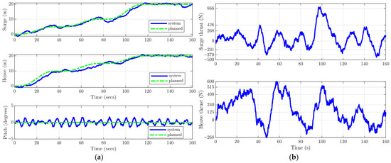
From Figure 11a, the RCTS is accurately tracking the planned trajectory in surge and heave. Moreover, the restoring hydrostatic moment keeps the pitch angle within ±3° under the effect of sensor and process noises.

Figure 11. RCTS while trajectory tracking under constraints: (a) translational and angular motion response; (b) thrust forces.

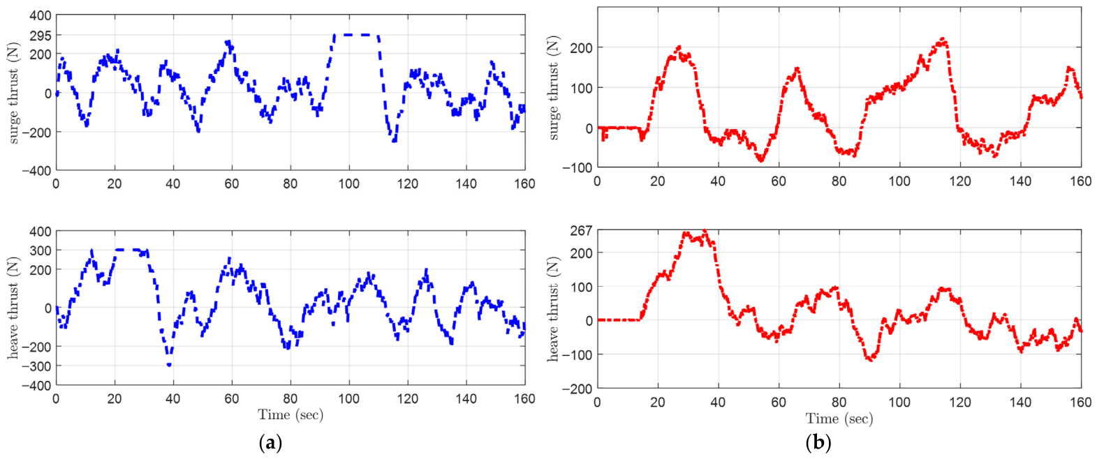
Figure 11b shows varying thrust forces while following the planned path under the NN controller. The maximum axial thrust force is applied between waypoints 3 and 4 of the planned path for RCTS as defined in Table 5, due to the longer distance that is required to be traveled in the same allocated segment time.

10.2. FCTS Response Under Sensor and Process Noise

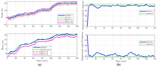
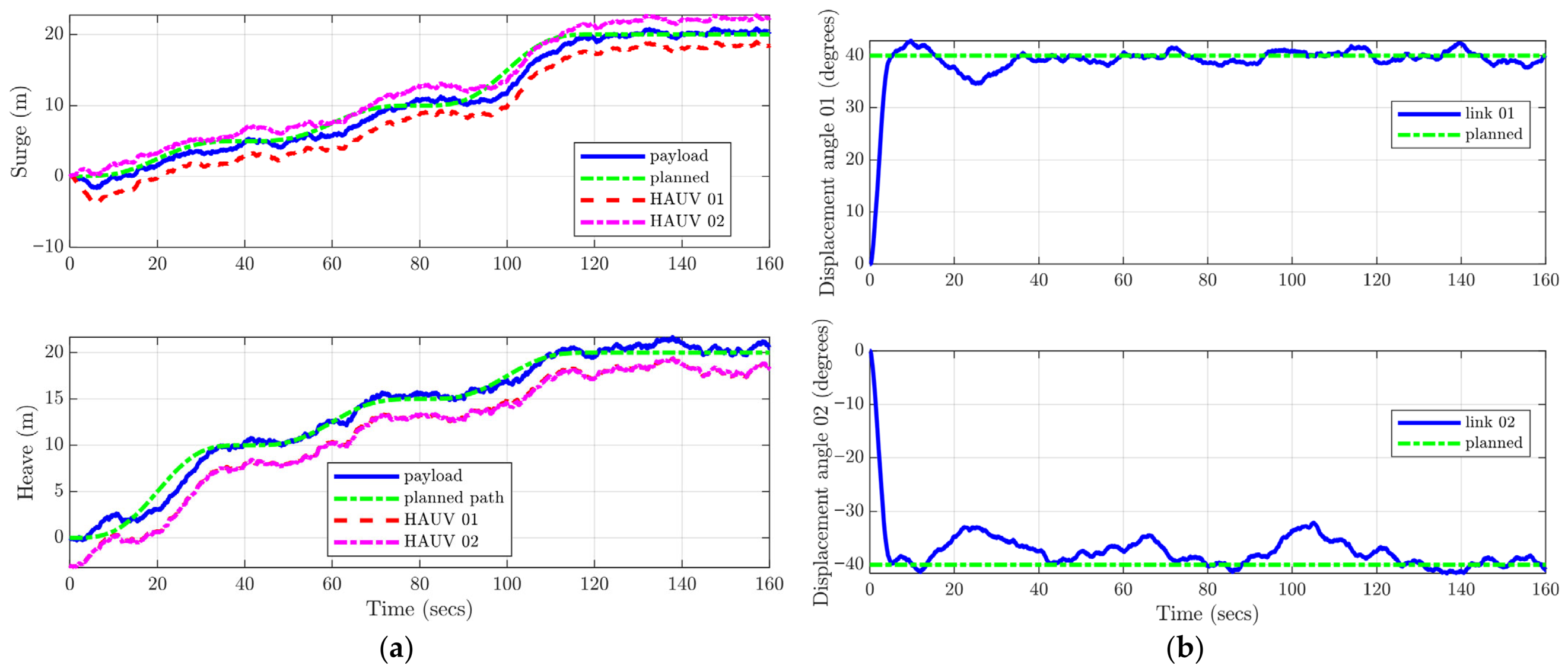
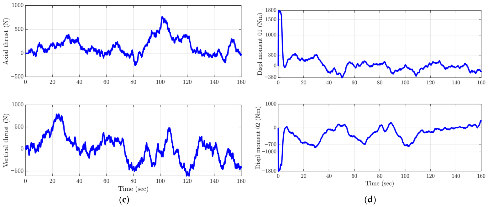
For the FCTS configuration, the system is tasked not only with trajectory tracking but also with maintaining displacement angles of +40° and −40° for flexible joint links 01 and 02, respectively, under the influence of sensor and process noise. As illustrated in Figure 12a, the planned path is followed accurately in both surge and heave directions. The required articulated link angles are achieved and sustained effectively, as shown in Figure 12b.

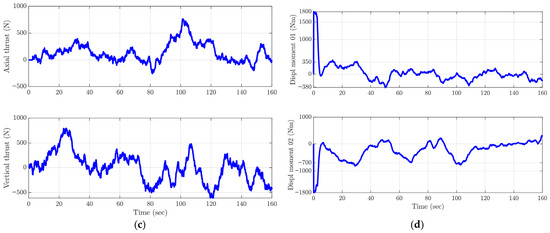
Figure 12. FCTS response during tracking of the desired trajectory under constraints: (a) surge and heave response; (b) articulated link angle; (c) force response by thrust actuators; (d) moment response by thrust actuators.

Figure 12c depicts the variations in thrust force as the system navigates each segment of the planned trajectory while preserving the specified link angles. Initially, displacement moments of ±1800 N are applied to set the desired angles of the links, as presented in Figure 12d. Subsequently, the thrust moments fluctuate dynamically to maintain the link displacements despite process and sensor disturbances.

10.3. LFFCTS Response Under Sensor and Process Noises

For the LFFCTS, sensor and process noises are separately applied to leader and follower HAUVs of the transportation system.

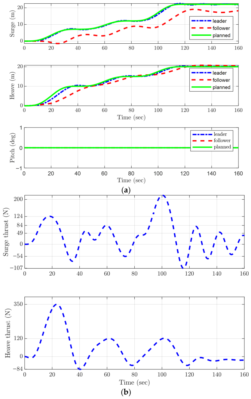
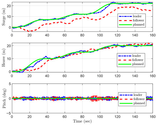
From Figure 13, the leader HAUV is accurately tracking the planned trajectory and the follower HAUV keeps its distance from the leader throughout the motion. The restoring hydrostatic moments efficiently keep the pitch angle of each vehicle of the LFFCTS near zero degrees under sensor and process noises.

Figure 13. Response of LFFCTS transportation configuration during trajectory tracking under constraints (motion response in surge, heave and pitch).

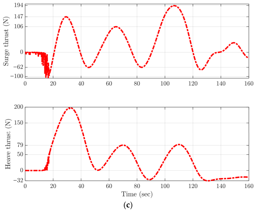
Figure 14a,b show the force response by the thrust actuators of the leader and follower HAUVs of the LFFCTS transportation configuration. The thrust force variation for the leader HAUV is higher than for the follower HAUV.

Figure 14. Response of LFFCTS transportation configuration during trajectory tracking under constraints: (a) thrust force response by the actuators of the leader HAUV; (b) thrust force response by the actuators of the follower HAUV.

Table 11 shows the RMSE values of the states for the three transportation systems under ideal conditions and under sensor and process noises. The RMSE values of surge and heave for the RCTS, FCTS, and leader HAUV of the LFFCTS have a maximum value of 1.03 m under ideal conditions and a maximum value of 1.22 m under process and sensor noises. Meanwhile, the RMSE values of surge and heave for the follower HAUV of the LFFCTS are comparatively higher at more than 2 m. This is due to the reason that the follower HAUV gets commands from the leader through the formation controller, which causes delays and inaccuracies. The RMSEs of the articulated link angles have a maximum value of 4.90° under ideal conditions and 5.13° under sensor and process noises, which is quite impressive with regard to controlling articulated link angles.

Table 12 shows the mean consumption of power by the transportation systems under ideal conditions and under the influence of sensor and process noises. The RCTS consumes the lowest power, whereas the power consumption of the LFFCTS is only 5% higher that the RCTS under ideal conditions and only 4% higher under sensor and process noises. The FCTS consumes the highest power due to its dynamic positioning problem.

The performance of autonomous underwater-transportation systems under NNAC is compared with the conventional PID controller, as summarized in Table 13, Table 14, Table 15 and Table 16. Table 13 and Table 14 indicate that NNAC achieves higher motion accuracy than conventional PID, as RMSEs across all configurations have reduced, with improvements ranging from 26% to 72%. This demonstrates clear superiority of NNAC over conventional PID in motion accuracy. The highest gains are observed in orientation control (up to 72% reduction), indicating NNAC’s strong capability in handling nonlinear heading dynamics and coupling effects. This confirms the robustness of NNAC for complex multi-vehicular systems and environmental constraints.

Table 13. Comparison of motion accuracy of RCTS and FCTS using conventional PID and NNAC.

	RCTS			FCTS
	Conventional PID	NNAC	Improvement (%)	Conventional PID	NNAC	Improvement (%)
${RMSE}_x$(m)	2.09	1.08	48.3	2.12	1.14	46.2
${RMSE}_z$(m)	3.05	1.22	60	3.11	1.01	67.5
${RMSE}_{\theta }$(o)	1.94	0.67	65.5	-	-	-
${RMSE}_{\lambda 1}$(o)	-	-	-	9.6	4.32	55.0
${RMSE}_{\lambda 2}$(o)	-	-	-	10.5	5.13	51.1

Table 14. Comparison of motion accuracy of LFFCTS using conventional PID and NNAC.

	LFFCTS
	Conventional PID		NNAC		% Improvement
	Leader	Follower	Leader	Follower	Leader	Follower
${RMSE}_x$ (m)	1.67	3.45	1.03	2.08	38.3	39.7
${RMSE}_z$ (m)	2.09	2.61	0.98	1.92	53.1	26.4
${RMSE}_{\theta }$ (o)	1.2	1.2	0.33	0.33	72.5	72.5
${RMSE}_{\lambda 1}$ (o)	-	-	-	-	-	-
${RMSE}_{\lambda 2}$ (o)	-	-	-	-	-	-

Table 15. Comparison of power consumption of RCTS and FCTS using conventional PID and NNAC.

	RCTS			FCTS
	Conventional PID	NNAC	% Increase	Conventional PID	NNAC	% Increase
${RMS}_X$(Watt)	86.21	124.3	39.7	57.64	86.6	33.4
${RMS}_Z$(Watt)	61.41	78.9	26.4	131.6	128.3	−2.6
${RMS}_M$(Watt)	0.0	0.0	0.0	0.0	0.0	0.0
${RMS}_{Q1}$(Watt)	-	-	-	14.92	43.8	65.9
${RMS}_{\mathrm{Q}2}$(Watt)	-	-	-	20.93	40.3	48.1
Total (Watt)	147.6	203.2	27.4%	225.1	299.0	24.7%

Table 16. Comparison of power consumption of LFFCTS using conventional PID and NNAC.

	LFFCTS
	Conventional PID		NNAC		% Increase
	Leader	Follower	Leader	Follower	Leader	Follower
${RMS}_X$(Watt)	41.12	32.14	63.2	54.0	34.9	40.5
${RMS}_Z$(Watt)	40.42	29.87	44.1	45.2	8.3	33.9
${RMS}_M$(Watt)	0.0	0.0	0.0	0.0	0	0
${RMS}_{Q1}$(Watt)	-	-	-	-	-	-
${RMS}_{\mathrm{Q}2}$(Watt)	-	-	-	-	-	-
Total (Watt)	122.62		206.5		40.6%

On the other hand, Table 15 and Table 16 show that the improvement in motion accuracy comes at the cost of an increase in power consumption. The increase in total power consumption is 25% to 41%. This additional energy directly contributes to much better motion accuracy, with RMSE reductions ranging from 26% to 72%. Since all thrust levels remain within the allowable actuator limits, the increased power demand remains safe and can be considered a reasonable trade-off for achieving more reliable and precise trajectory tracking in multi-vehicular underwater transportation.

Overall, the RCTS demonstrated the highest tracking accuracy while consuming the least power, which can be attributed to its treatment as a single rigid body with zero motion between system parts. In contrast, the FCTS required substantially higher control gains to regulate articulated link angles. These links, being hinged to the payload and vehicles, exhibit sensitive relative dynamics akin to a complex dynamic positioning system, resulting in persistent oscillations even under elevated gain settings. The follower HAUV in the LFFCTS exhibited the lowest motion accuracy, as it relies on the leader HAUV’s states through the formation controller. The indirect and continuously varying input from the leader introduces delays and inaccuracies in follower control. Additionally, the FCTS incurred the highest power consumption due to the demands of its intricate dynamic positioning requirements.

11. Conclusions

This study addresses a gap in the literature by applying Neural Network-Augmented Control (NNAC) to multi-vehicle autonomous underwater-transportation systems, integrated with an Extended Kalman Filter (EKF) state estimator under sensor and process noise conditions. The NN utilized both forward and backward propagation, demonstrating robustness in achieving precise motion responses even in the presence of disturbances. Comparison between NNAC and conventional PID indicates that the transportation system under NNAC achieves higher trajectory tracking accuracy, albeit with increased actuator effort. This trade-off is acceptable provided the thrusters operate within their permissible limits.

Overall, the RCTS exhibited superior performance and robustness compared to the LFFCTS and FCTS, particularly in terms of motion accuracy and minimal thruster actuation requirements.

Nevertheless, the flexibility offered by the LFFCTS and FCTS is critical for navigating narrow channels or re-configuring HAUVs to avoid scattered obstacles, which might not be possible with the rigid structure of the RCTS configuration. Between these two configurations, the LFFCTS achieved better motion precision with lower thrust efforts and power consumption, whereas the FCTS required the highest control efforts and power due to the highly sensitive dynamics of its articulated links.

It can be concluded that the RCTS is the most suitable option while operating in deep waters with no narrow channels and scattered obstacles. Whereas, for constrained environments with narrow channels and scattered obstacles, where positional adjustment of the vehicles is required, the LFFCTS is better suited. The FCTS is comparatively a less viable option due to its higher power consumption and lower motion and control accuracy.

Future work may explore more advanced intelligent controllers for these transportation systems, evaluating thrust efficiency and actuator performance across configurations.

Appendix A.1. RCTS Under Ideal Conditions

Figure A1. RCTS response while tracking the desired trajectory under ideal conditions; (a) translational and angular motion response; (b) thrust forces.

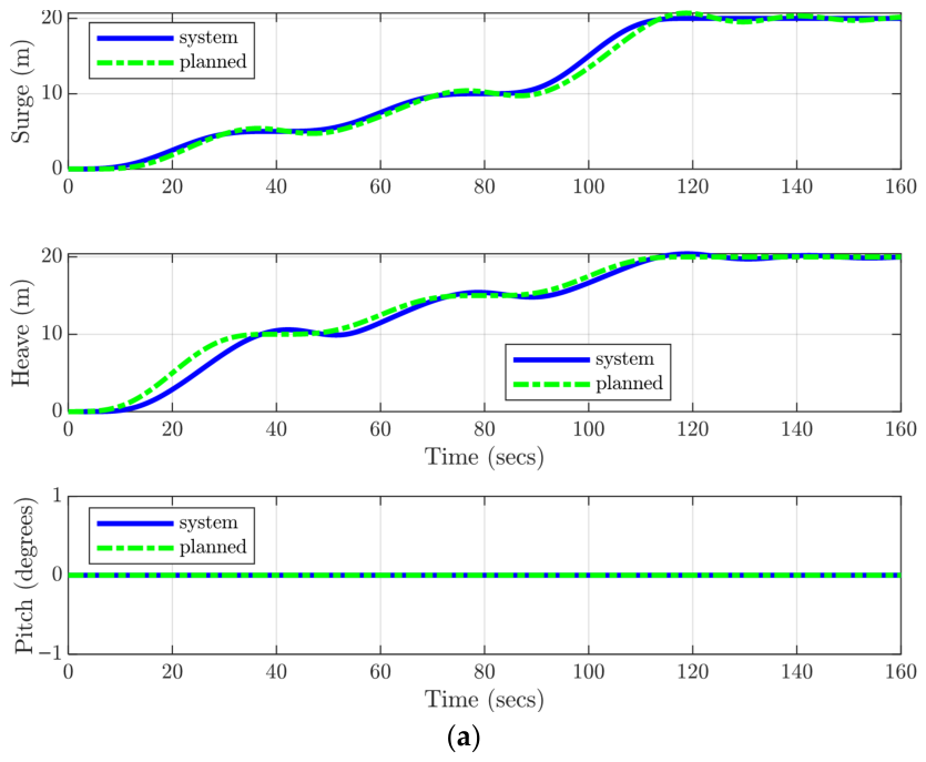
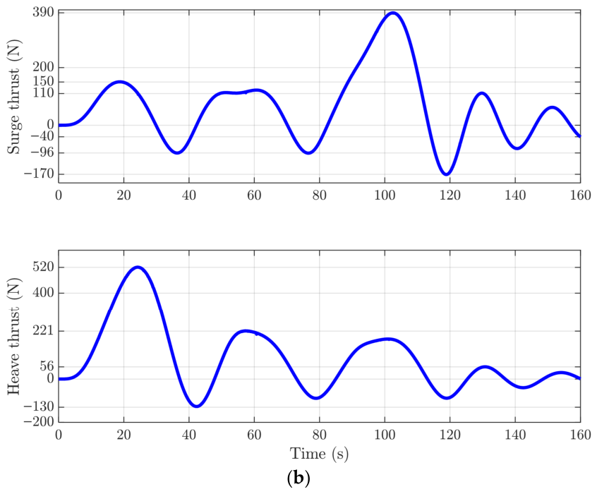
Figure A1. RCTS response while tracking the desired trajectory under ideal conditions; (a) translational and angular motion response; (b) thrust forces.

Appendix A.2. FCTS Under Ideal Conditions

Figure A2. FCTS response while tracking the desired trajectory under ideal conditions; (a) translational motion response; (b) displacement angle response; (c) thrust force response; (d) thrust moment response.

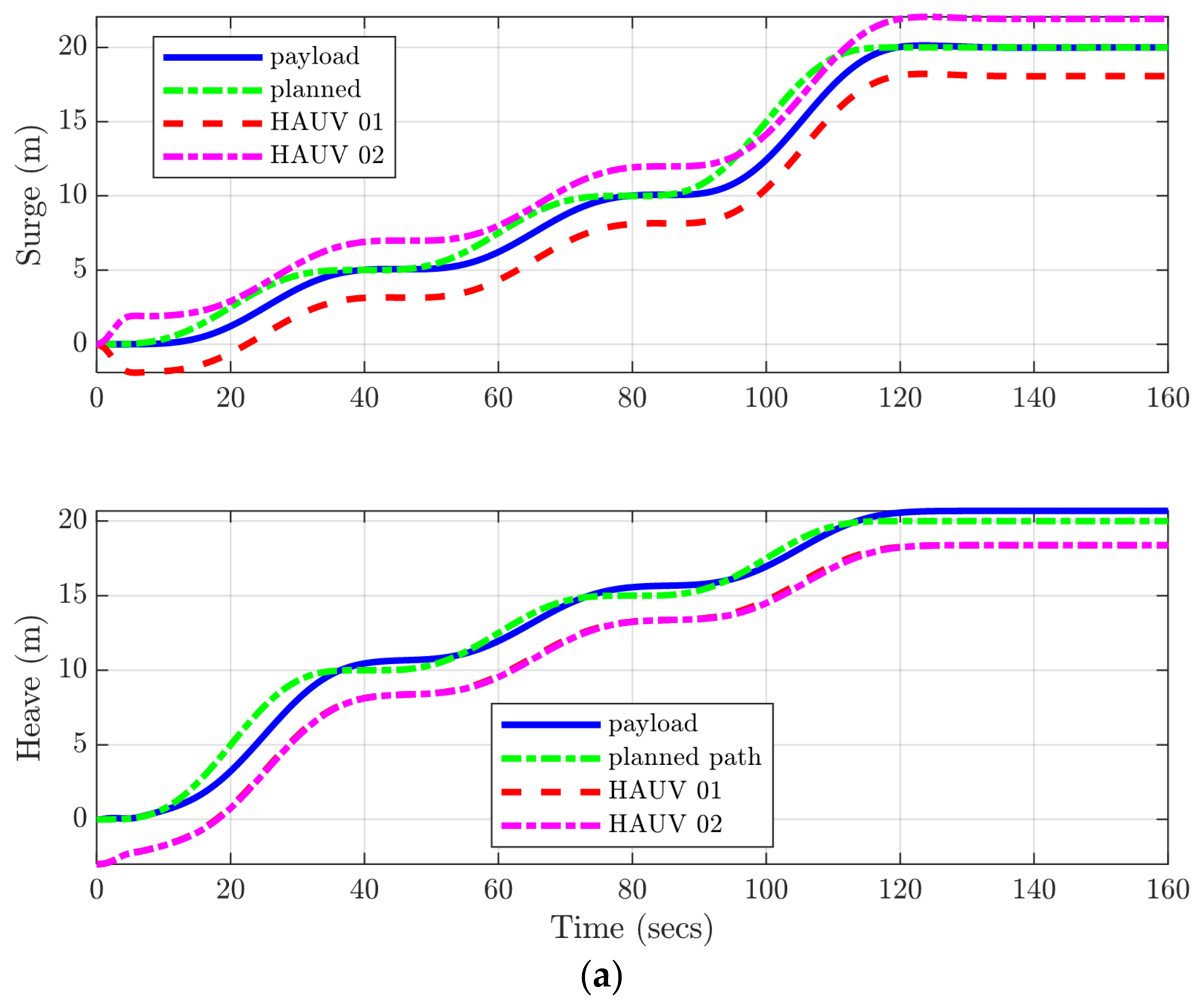
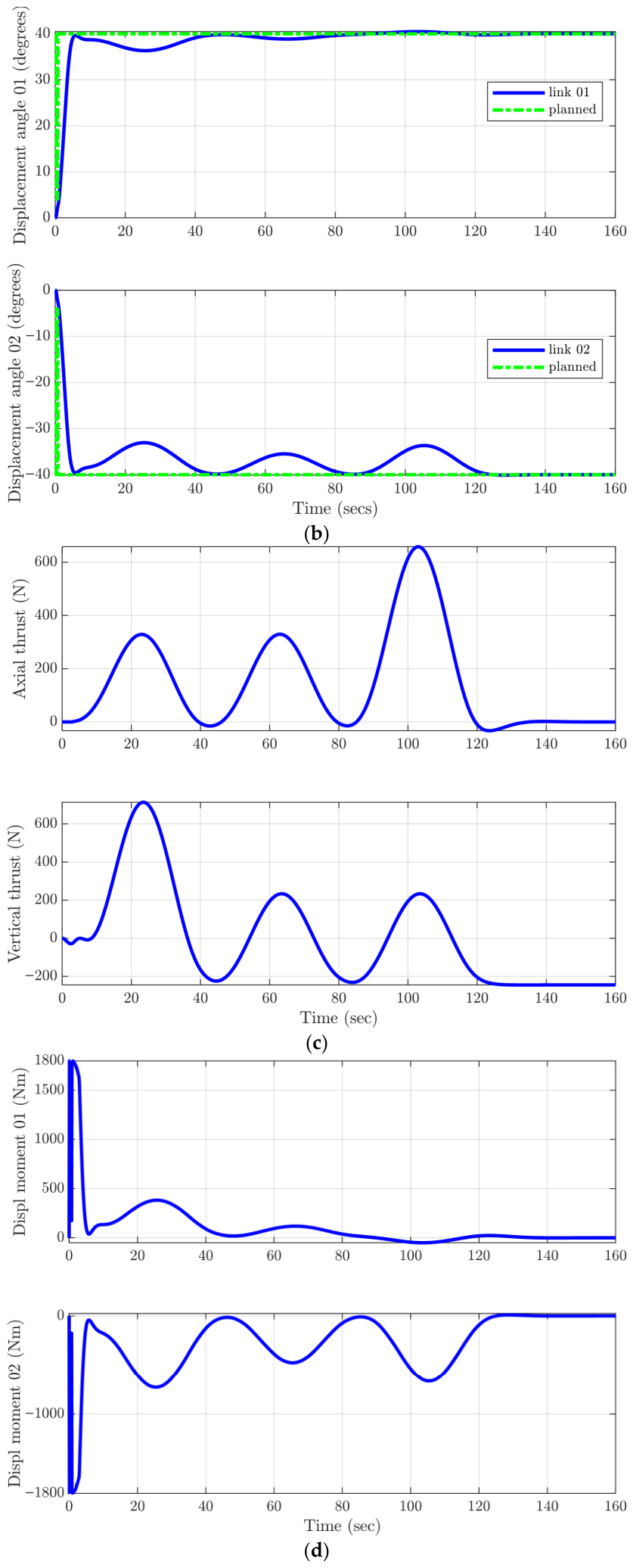
Figure A2. FCTS response while tracking the desired trajectory under ideal conditions; (a) translational motion response; (b) displacement angle response; (c) thrust force response; (d) thrust moment response.

Appendix A.3. LFFCTS Under Ideal Conditions

Figure A3. LFFCTS response while tracking the desired trajectory under ideal conditions; (a) translational motion response; (b) thrust response of the leader HAUV; (c) thrust response of the follower HAUV.

Figure A3. LFFCTS response while tracking the desired trajectory under ideal conditions; (a) translational motion response; (b) thrust response of the leader HAUV; (c) thrust response of the follower HAUV.

References

- Rehman, F.U. Underwater-Transportation of a Payload Using Multiple Hovering Autonomous Underwater Vehicles (HAUVs). Ph.D. Thesis, University College London, London, UK, 2024. Available online: https://discovery.ucl.ac.uk/id/eprint/10185963 (accessed on 11 December 2025).
- Ahmadabadi, M.N.; Nakano, E. A ‘constrain and move’ approach to distributed object manipulation. IEEE Trans. Robot. Autom. 2001, 17, 157–172. [Google Scholar] [CrossRef]
- Zaerpoora, A.; Nili, M. Distributed object transportation on a desired path based on Constrain and Move strategy. Robot. Auton. Syst. 2005, 50, 115–128. [Google Scholar] [CrossRef] [Scilit]
- Lee, H.; Kim, H.; Kim, H.J. Planning and Control for Collision-Free Cooperative Aerial Transportation. IEEE Trans. Autom. Sci. Eng. 2018, 15, 189–201. [Google Scholar] [CrossRef] [Scilit]
- Mellinger, D. Trajectory Generation and Control for Quadrotors. Mechanical Engineering and Applied Mechanics. Ph.D. Thesis, University of Pennsylvania, Philadelphia, PA, USA, 2012. [Google Scholar]
- Rehman, F.U.; Thomas, G.; Anderlini, E. Development of a Simulation Platform for underwater-transportation using two Hovering Autonomous Underwater Vehicles (HAUVs). In Proceedings of the 6th International Conference of Control, Dynamic Systems, and Robotics (CDSR’19), Ottawa, ON, Canada, 6–7 June 2019; pp. 1–8. [Google Scholar] [CrossRef] [Scilit]
- Rehman, F.U.; Thomas, G.; Anderlini, E. Centralized Control System Design for underwater-transportation using two Hovering Autonomous Underwater Vehicles (HAUVs). IFAC-PapersOnLine 2019, 52, 13–18. [Google Scholar] [CrossRef] [Scilit]
- Bernard, M.; Kondak, K. Generic Slung Load Transportation System Using Small Size Helicopters. In IEEE International Conference on Robotics and Automation (ICRA); IEEE: New York, NY, USA, 2009; pp. 3258–3264. [Google Scholar] [CrossRef] [Scilit]
- Li, Z.; Horn, J.F.; Langelaan, J.W. Coordinated Transport of a Slung Load by a Team of Autonomous Rotorcraft. In AIAA Guidance, Navigation, and Control Conference; AIAA SciTech: Reston, VA, USA, 2014; pp. 1–23. [Google Scholar]
- Michael, N.; Fink, J.; Kumar, V. Cooperative manipulation and transportation with aerial robots. Auton. Robot. 2010, 30, 73–86. [Google Scholar] [CrossRef] [Scilit]
- Oh, S.-R.; Ryu, J.-C.; Agrawal, S.K. Dynamics and Control of a Helicopter Carrying a Payload Using a Cable-Suspended Robot. J. Mech. Des. 2006, 128, 1113–1121. [Google Scholar] [CrossRef] [Scilit]
- Goodarzi, F.A.; Lee, D.; Lee, T. Geometric Stabilization of a Quadrotor UAV with a Payload Connected by Flexible Cable. In American Control Conference; IEEE: New York, NY, USA, 2014; pp. 4925–4930. [Google Scholar] [CrossRef] [Scilit]
- Yufka, A.; Ozkan, M. Formation-Based Control Scheme for Cooperative Transportation by Multiple Mobile Robots. Int. J. Adv. Robot. Syst. 2015, 12, 120. [Google Scholar] [CrossRef] [Scilit] [PubMed]
- Lysdahl, C. Design of Dynamic Positioning System for ROV Minerva. Master’s Thesis, Norwegian University of Science and Technology, Trondheim, Norway, 2010. [Google Scholar]
- Holven, E.B. Control System for ROV Minerva 2. Master’s Thesis, Norwegian University of Science and Technology, Trondheim, Norway, 2018. [Google Scholar]
- Mo, S.M. Development of a Simulation Platform for ROV Systems. Master’s Thesis, Norwegian University of Science and Technology, Trondheim, Norway, 2015. [Google Scholar]
- Rehman, F.U.; Anderlini, E.; Thomas, G.; Ali, A. Multivehicular underwater-transportation using Flexible-Connections. In International Conference on Smart Ship Technology; Royal Institue of Naval Architects: London, UK, 2020; pp. 41–51. [Google Scholar]
- Moonesun, M.; Ghasemzadeh, F.; Valeri, N.; Yastreba, A.; Ursalov, A. Effective Depth of Regular Wave on Submerged Submarines and AUVs. Int. Robot. Autom. J. 2017, 2, 208–216. [Google Scholar] [CrossRef] [Scilit]
- Fossen, T.I. Handbook of Marine Craft Hydrodynamics and Motion Control, 1st ed.; John Wiley & Sons: Hoboken, NJ, USA, 2011. [Google Scholar]
- Guo, M.; Su, Y.; Gu, D. Mixed H2/H∞ Tracking Control with Constraints for Single Quadcopter Carrying a Cable-suspended Payload. IFAC-PapersOnLine 2015, 50, 4869–4874. [Google Scholar] [CrossRef] [Scilit]
- Rehman, F.U.; Anderlini, E.; Thomas, G. The Impact of Sea Current on underwater-transportation using Four AUVs. In International Conference on Autonomous Ships; Royal Institue of Naval Architects: London, UK, 2020; pp. 49–58. [Google Scholar]
- Yan, Z.; Liu, Y.; Zhou, J.; Wu, D. Path following control of an AUV under the current using the SVR-ADRC. J. Appl. Math. 2014, 12, 476419. [Google Scholar] [CrossRef] [Scilit]
- Aguiar, A.P.; Pascoal, A.M. Dynamic positioning of an underactuated auv in the presence of a constant unknown ocean current disturbance. IFAC Proc. Vol. 2002, 35, 283–288. [Google Scholar] [CrossRef] [Scilit]
- Luo, J.; Tang, Z.; Peng, Y.; Xie, S.; Cheng, T.; Li, H. Anti-disturbance Control for an Underwater Vehicle In Shallow Wavy Water. Adv. Control Eng. Inf. Sci. 2011, 15, 915–921. [Google Scholar] [CrossRef] [Scilit]
- Dantas, J.L.D.; Da Cruz, J.J.; De Barros, E.A. Study of autonomous underwater vehicle wave disturbance rejection in the diving plane. J. Eng. Marit. Environ. 2014, 228, 122–135. [Google Scholar] [CrossRef] [Scilit]
- Zhao, F.Z.; Song, B.W.; Du, X.X. Simulation and Analysis of AUV’s Hydrodynamics When Moving in the Near-Seabed. Adv. Mat. Res. 2012, 605–607, 2409–2412. [Google Scholar] [CrossRef] [Scilit]
- Randeni, S.A.T.P.; Leong, Z.Q.; Ranmuthugala, D.; Forrest, A.L.; Duffy, J. Numerical investigation of the hydrodynamic interaction between two underwater bodies in relative motion. Appl. Ocean Res. 2015, 51, 14–24. [Google Scholar] [CrossRef] [Scilit]
- Leong, Z.Q.; Ranmuthugala, D.; Penesis, I.; Nguyen, H. Quasi-static analysis of the hydrodynamic interaction effects on an autonomous underwater vehicle operating in proximity to a moving submarine. Ocean Eng. 2015, 106, 175–188. [Google Scholar] [CrossRef] [Scilit]
- Leong, Z.Q. Effects of Hydrodynamic Interaction on an AUV Operating Close to a Moving Submarine. Ph.D. Thesis, Australian Maritime College, University of Tasmania, Tasmania, Australia, 2014. [Google Scholar]
- Zhang, Y.; Wang, L. Real-Time Disturbances Estimating and Compensating of Nonlinear Dynamic Model for Underwater Vehicles. Math. Probl. Eng. 2018, 16, 3073072. [Google Scholar] [CrossRef] [Scilit]
- Huang, B.; Yang, Q. Depth Control of ROVs based on disturbance observer and double-loop sliding mode controller. In Proceedings of the Twenty-Ninth International Ocean and Polar Engineering Conference; International Society of Offshore and Polar Engineers: Cupertino, CA, USA, 2019; pp. 1609–1615. [Google Scholar]
- Londhe, P.S.; Dhadekar, D.D.; Patre, B.M.; Waghmare, L.M. Uncertainty and disturbance estimator based sliding mode control of an autonomous underwater vehicle. Int. J. Dyn. Control 2017, 5, 1122–1138. [Google Scholar] [CrossRef] [Scilit]
- Kalman, R.E. A new approach to linear filtering and prediction problems. J. Fluids Eng. 1960, 82, 35–45. [Google Scholar] [CrossRef] [Scilit]
- Grewal, M.S. Kalman filtering. In International Encyclopedia of Statistical Science; Springer: Berlin/Heidelberg, Germany, 2011; pp. 705–708. [Google Scholar]
- Welch, G.; Bishop, G. An Introduction to the Kalman Filter; University of North Carolina at Chapel Hill: Chapel Hill, NC, USA, 2006; Available online: https://www.cs.unc.edu/~welch/media/pdf/kalman_intro.pdf (accessed on 26 April 2026).
- Karras, G.C.; Panagou, D.J.; Kyriakopoulos, K.J. Localization of an underwater vehicle using an IMU and a laser-based vision system. In Proceedings of the 15th Mediterranean Conference on Control & Automation; IEEE: New York, NY, USA, 2007. [Google Scholar] [CrossRef] [Scilit]
- Brunton, S.L.; Kutz, J.N. Data Driven Science Engineering (Machine Learning, Dynamical Systems, and Control); Cambridge University Press: Cambridge, UK, 2017. [Google Scholar]
- Keatmanee, C.; Baber, J.; Bakhtyar, M. Simple Example of Applying Extended Kalman Filter. In Proceedings of the 1st International Electrical Engineering Congress (iEECON), Chiang Mai, Thailand, 13–15 March 2013; pp. 1–4. [Google Scholar]
- Steinke, D.M.; Buckham, B.J. A Kalman filter for the navigation of remotely operated vehicles. In Proceedings of MTS/IEEE OCEANS; IEEE: New York, NY, USA, 2005; pp. 1–8. [Google Scholar] [CrossRef] [Scilit]
- Dekking, F.M.; Kraaikamp, C.; Lopuhaa, H.P.; Meester, L.E. Expectation and variance. In A Modern Introduction to Probability and Statistics; Springer: London, UK, 2005. [Google Scholar]
- Martínez, B.V.; Sierra, D.A.; Villamizar, R. Navigation of an Underwater Remotely Operated Vehicle based on Extended Kalman Filter. In Proceedings of the ASME 2013 Dynamic Systems and Control Conference, DSCC, Palo Alto, CA, USA, 21–23 October 2013; p. 9. [Google Scholar] [CrossRef] [Scilit]
- Mellinger, D.; Kumar, V. Minimum Snap Trajectory Generation and Control for Quadrotors. In IEEE International Conference on Robotics and Automation; IEEE: New York, NY, USA, 2011; pp. 2520–2525. [Google Scholar]
- Salmalian, K.; Soleimani, M. ANFIS and neural network for modeling and prediction of ship squat in shallow waters. Int. J. Math. Models Methods Appl. Sci. 2011, 5, 848–856. [Google Scholar]
- Royce, R.A.; Mouravieff, A.; Zuzick, A. Trimaran Resistance Artificial Neural Network. In Proceedings of the 11th International Conference on Fast Sea Transportation (FAST 2011), Honolulu, HI, USA, 26–29 September 2011; pp. 717–726. [Google Scholar]
- Gougoulidis, G. The Utilization of Artificial Neural Networks in Marine Applications: An Overview. Nav. Eng. J. 2008, 120, 19–26. [Google Scholar] [CrossRef] [Scilit]
- Couser, P.; Mason, A.; Mason, G.; Smith, C.R.; Von Konsky, B.R. Artificial Neural Networks for Hull Resistance Prediction. In Proceedings of the 3rd International Conference on Computer Applications and Information Technology in the Marine Industries (COMPIT), Siguenza, Spain, 9–12 May 2004; pp. 391–402. [Google Scholar]
- Khan, H. Artificial Neural Networks Based Prediction And Validation Tool (Annpvt) For Ship Model Powering Tests In Towing Tanks. In 2021 International Conference on Artificial Intelligence (ICAI); IEEE: New York, NY, USA, 2021; pp. 113–118. [Google Scholar] [CrossRef] [Scilit]
- Tannuri, E.A.; Kubota, L.K.; Pesce, C.P. Adaptive techniques applied to offshore dynamic positioning systems. J. Braz. Soc. Mech. Sci. Eng. 2006, 28, 323–330. [Google Scholar] [CrossRef] [Scilit]
- Xu, S.; Wang, X.; Yang, J.; Wang, L. A fuzzy rule-based PID controller for dynamic positioning of vessels in variable environmental disturbances. J. Mar. Sci. Technol. 2020, 25, 914–924. [Google Scholar] [CrossRef] [Scilit]
- Khan, H. Efficient Design and Analysis of Battery Switching Stations for the Collaborative Wireless Network of Mobile Robots. In 2021 International Conference on Artificial Intelligence (ICAI); IEEE: New York, NY, USA, 2021; pp. 198–202. [Google Scholar] [CrossRef] [Scilit]
- Skulstad, R.; Li, G.; Zhang, H.; Fossen, T.I. A Neural Network Approach to Control Allocation of Ships for Dynamic Positioning. FAC-PapersOnLine 2018, 51, 128–133. [Google Scholar] [CrossRef] [Scilit]
- Øvereng, S.S.; Nguyen, D.T.; Hamre, G. Dynamic Positioning using Deep Reinforcement Learning. Ocean Eng. 2021, 235, 109433. [Google Scholar] [CrossRef] [Scilit]
- Liang, X.; Li, J. ESO-Enhanced Actor–Critic Reinforcement Learning-Optimised Trajectory Tracking Control for 3-DOF Marine Vessels. Mathematics 2026, 14, 867. [Google Scholar] [CrossRef] [Scilit]
- Liang, X.; Li, J.; Bao, D. Fixed-Time Event-Triggered Control for Distributed Unmanned Underwater Vehicles. J. Mar. Sci. Eng. 2026, 14, 202. [Google Scholar] [CrossRef] [Scilit]
- Rehman, F.U.; Khan, H.; Aijun, L.; Malik, S.A.; Mahmood, S.; Ali, A. Evaluation of Multi-Vehicular underwater-transportation Systems under Disturbances, Sensor Noise and Limited Sensor Readings. In 2022 19th International Bhurban Conference on Applied Sciences and Technology (IBCAST); IEEE: New York, NY, USA, 2022; pp. 905–917. [Google Scholar] [CrossRef] [Scilit]
- Morgado, M.; Batista, P.; Oliveira, P.; Silvestre, C. Position and Velocity USBL/IMU Sensor-based Navigation Filter. IFAC Proc. Vol. 2011, 44, 13642–13647. [Google Scholar] [CrossRef] [Scilit]
- Bayat, M.; Aguiar, A.P. SLAM for an AUV using vision and an acoustic beacon. IFAC Proc. Vol. 2010, 43, 503–508. [Google Scholar] [CrossRef] [Scilit]
- Abdel-Hafez, M.F. On the GPS/IMU sensors’ noise estimation for enhanced navigation integrity. Math. Comput. Simul. 2012, 86, 101–117. [Google Scholar] [CrossRef] [Scilit]
- Shanmugam, G. New Perspectives on Deep-water Sandstones. In Handbook of Petroleum Exploration and Production; Elsevier: Amsterdam, The Netherlands, 2012. [Google Scholar]
Disclaimer/Publisher’s Note: The statements, opinions and data contained in all publications are solely those of the individual author(s) and contributor(s) and not of MDPI and/or the editor(s). MDPI and/or the editor(s) disclaim responsibility for any injury to people or property resulting from any ideas, methods, instructions or products referred to in the content. |
© 2026 by the authors. Licensee MDPI, Basel, Switzerland. This article is an open access article distributed under the terms and conditions of the Creative Commons Attribution (CC BY) license.