Asymptotic Stabilization Control Based on Trajectory Optimization for Vertical Underactuated Manipulators with the First Joint Actuator

Abstract

Underactuated system control is a central topic in nonlinear system control. For the three-link vertical underactuated manipulator with only the first joint actuated (APP manipulator), the control objective of swing-up and balancing is challenging. The advantages of this paper are as follows: (i) The proposed method avoids balancing region division in common partitioned control, preventing failure to stabilize at the target position due to improper partitioning. (ii) The time-based switching condition optimized via parameter tuning is easier to satisfy than the state-based condition. (iii) The proposed controller effectively suppresses state fluctuations caused by switching, yielding a smoother transition. (iv) The proposed controller avoids the singularity problem. The main procedures are as follows. First, the dynamic model of the APP manipulator is established. Then, a trajectory is designed to guide the active link from the initial position to the vicinity of the target position. On this basis, to ensure that all links can simultaneously reach the vicinity of the target position, the trajectory parameters are optimized according to the coupling relationship between the links. Next, an NFTSM-based tracking controller is developed to steer the links along the optimized trajectory. After that, an LQR-based stabilization controller is further employed to lock the system at the target position. Finally, the effectiveness of the proposed method is verified through simulations.

1. Introduction

Underactuated systems are a class of nonlinear systems in which the number of inputs is less than the number of degrees of freedom [1]. Many existing systems fall into this category, such as ship-mounted cranes [2,3], surface ships [4,5], and robots that have been widely and increasingly applied across various fields in recent years [6,7]. Due to their advantages of flexible control and energy efficiency, underactuated systems possess significant theoretical and engineering value in nonlinear control.

A robotic manipulator is a typical underactuated system. The passive links of the manipulator cannot be directly controlled due to the absence of corresponding actuators. Furthermore, the dynamic equations of the passive links are non-integrable, which makes the system subject to second-order nonholonomic constraints [8,9]. Additionally, the strong coupling relationship between links tends to induce singularities during motion [10], which makes controlling underactuated manipulators particularly challenging. This paper focuses on a three-link vertical manipulator with only the first joint actuated (APP manipulator) Compared with systems such as the Pendubot [11,12] and the Acrobot [13], the vertical APP manipulator exhibits more complex nonlinearities and coupling relationships, and is more prone to singularities during the swing-up process, making control of such system even more difficult.

For vertical manipulators, the control objective is to swing them up from the vertically downward initial position (DIP), finally stabilize them at the vertically upward target position (UTP) [14,15]. At present, the partitioned control approach is widely adopted to achieve this control objective [16]. The core of this approach is to divide the motion space into a swing-up region and a balancing region, and design controllers separately to accomplish swing-up and stabilization control. Methods for designing the swing-up region controller include energy-based approaches [17], fuzzy control-based approaches [18], etc. For the balancing region, the linear quadratic regulator (LQR) [19] or pole placement method [20] is commonly used to design the stabilization controller. The control objective is then achieved by switching controllers between the swing-up region and the balancing region.

Although the aforementioned partitioned control approach is efficient in many cases, there is still no unified criterion for the division of the balancing region, which makes the state-based switching condition difficult to satisfy. If this region is set excessively large, it can easily lead to abrupt torque variation and even failure of stabilization. If this region is set excessively small, the switching condition will be difficult to satisfy. Moreover, the system cannot be guaranteed to enter the balancing region reliably, which may result in excessive control time. In addition, the strong coupling relationship and inherent nonlinearity of the system tend to introduce singular behaviors during the swing-up phase.

Trajectory planning is also a common approach in switched control [21,22]. Compared with traditional methods, such as energy-based control, this approach avoids complex motion decoupling and simplifies the controller design [23]. Trajectory planning mainly consists of two key stages: Trajectory optimization and tracking. (1) For trajectory optimization, an effective strategy is to employ intelligent optimization algorithms to find trajectory parameters that satisfy the control constraints. Typical examples include the genetic algorithm [24] and the particle swarm optimization algorithm [25]. Such intelligent optimization methods provide valuable insights for the design proposed in this paper. (2) For trajectory tracking, traditional nonlinear sliding mode (SM) control is widely adopted [26], but it cannot achieve finite-time convergence and exhibits a slow convergence rate.To address this limitation, researchers have successively proposed terminal sliding mode (TSM) control [27,28], non-singular terminal sliding mode (NTSM) control [29,30], and non-singular fast terminal sliding mode (NFTSM) control [31,32]. Among these methods, NFTSM can not only effectively eliminate singularities, but also accelerate the convergence of tracking errors. By introducing a continuous boundary layer into the NFTSM control law, the chattering phenomenon can be significantly suppressed, thereby effectively eliminating fluctuations during controller switching.

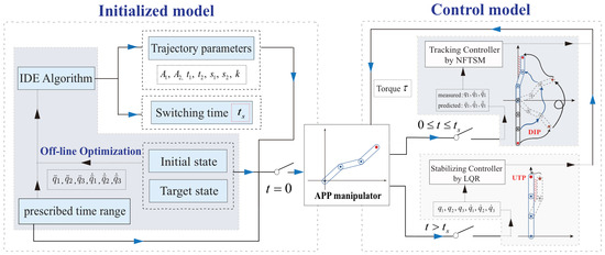
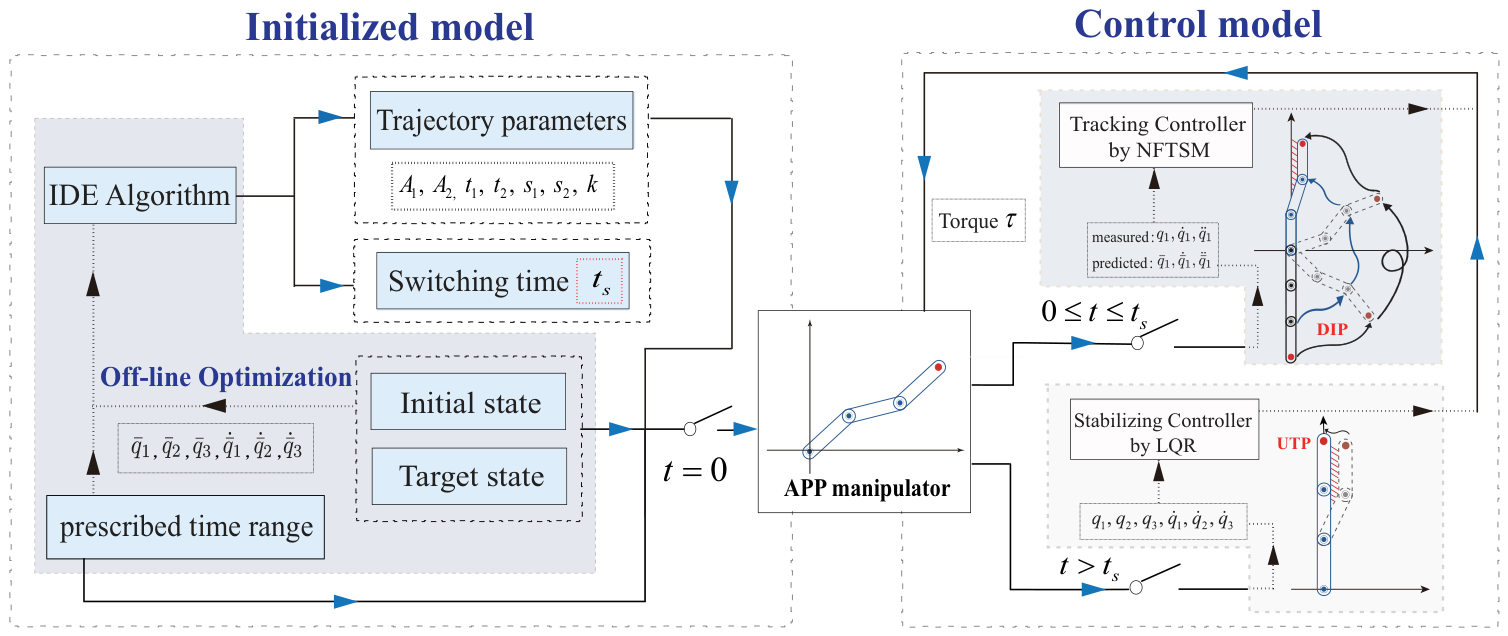
For vertical APP manipulators, this paper proposes an asymptotic stabilization control strategy based on partitioned control and trajectory optimization. The control structure is shown in Figure 1. First, a single trajectory is designed for the active link to swing directly from the DIP to the vicinity of the UTP. Subsequently, by incorporating the coupling relationship between the active and passive links, an improved differential evolution (IDE) algorithm is adopted to perform offline optimization of the trajectory parameters, thereby guaranteeing that all links reach the vicinity of the UTP simultaneously. An NFTSM-based tracking controller is applied to swing up the links along the optimized trajectory. As the system approaches the UTP, the controller is switched to an LQR-based stabilization controller, which compensates for gravitational disturbances and maintains steady-state balance.

Figure 1. Control Structure of Asymptotic Stabilization Control for APP Based on Trajectory Optimization.

The main advantages of this paper are summarized as follows:

• Compared with the traditional partitioned method, the proposed trajectory can directly swing the system up to the vicinity of the UTP, thus avoiding the difficulty of balancing region division via trajectory optimization.
• Compared with energy-based control methods, the proposed time-based switching condition is easier to satisfy than the state-based switching condition, always ensuring the system enters the balancing region and achieves stable control within a relatively short time.
• Compared with SM-based controllers, the NFTSM-based controller can effectively suppress state fluctuations during controller switching, thus achieving a smoother switching process.
• The proposed method effectively avoids the singularity problem.

2. System Dynamic Model

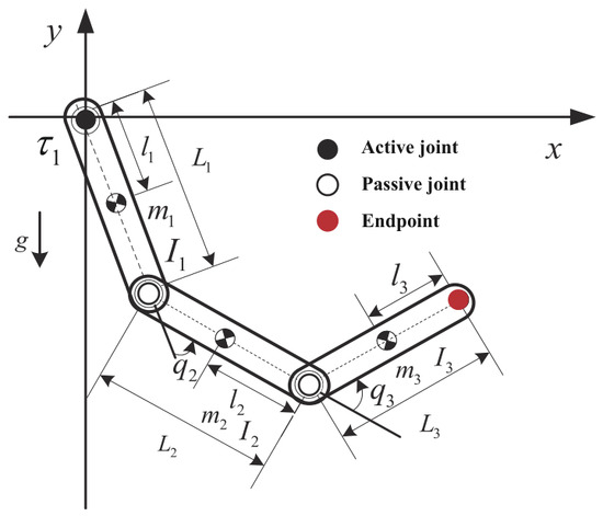
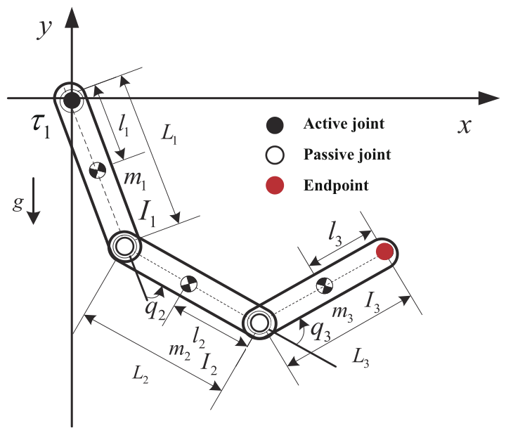
The structure of the APP manipulator is shown in Figure 2. Let the mass, length, and moment of inertia about the center of mass of the i-th $(i=1,2,3)$ link be $m_i$, $L_i$ and $J_i$, respectively. In addition, $L_{ci}$ denotes the distance from the i-th joint to the center of mass of this link, and g is the gravitational acceleration.

Figure 2. Structure of the APP manipulator.

The dynamic model of this system can be established via the Lagrange equation. Selecting the generalized coordinates as the joint angles $q={\left[q_1,q_2,q_3\right]}^T$, the dynamic equation of the system can be expressed in the following form:

$$M\left(q\right)\ddot{q}+C(q,\dot{q})\dot{q}+G\left(q\right)=\tau$$

(1)

where $M\left(q\right)\in R^{3\times 3}$ is a positive definite and symmetric inertia matrix, $C(q,\dot{q})\dot{q}\in R^{3\times 1}$ represents the Coriolis and centrifugal force vector, and $G\left(q\right)\in R^{3\times 1}$ is the gravitational force vector. Their structures are given as follows:

$$M\left(q\right)=\left[\begin{array}{ccc}{M}_{11}& M_{12}& M_{13}\\ M_{21}& M_{22}& M_{23}\\ M_{31}& M_{32}& M_{33}\end{array}\right],C(q,\dot{q})\dot{q}+G\left(q\right)=\left[\begin{array}{c}{H}_1\\ H_2\\ H_3\end{array}\right]$$

(2)

These expressions can be found in [33]. The joint torque is given by $\tau ={\left[{\tau }_1,0,0\right]}^T$, where only the first joint torque is non-zero, reflecting the underactuated characteristic of the APP manipulator. Substituting Equation (2) into Equation (1) gives:

$$\{\begin{array}{}\mathrm{(3a)}& M_{11}{\ddot{q}}_1+M_{12}{\ddot{q}}_2+M_{13}{\ddot{q}}_3+H_1={\tau }_1\mathrm{(3b)}& M_{21}{\ddot{q}}_1+M_{22}{\ddot{q}}_2+M_{23}{\ddot{q}}_3+H_2=0\mathrm{(3c)}& M_{31}{\ddot{q}}_1+M_{32}{\ddot{q}}_2+M_{33}{\ddot{q}}_3+H_3=0\end{array}$$

Equations (3b) and (3c) reveal the coupling relationship between active and passive links, which is crucial for controller design and analysis. To facilitate subsequent control analysis and simulation implementation, define the state vector as $x={[x_1,x_2,x_3,x_4,x_5,x_6]}^T$, then the system can be expressed in the standard state-space form:

$$\begin{array}{cc}\hfill & \left\{\begin{array}{cc}\hfill {\dot{x}}_1& =x_4,\hfill \\ \hfill {\dot{x}}_2& =x_5,\hfill \\ \hfill {\dot{x}}_3& =x_6,\hfill \end{array}\right.\hfill \end{array}$$

(4a)

$$\begin{array}{cc}\hfill {\dot{x}}_{4:6}& =F\left(x\right)+B\left(x\right){\tau }_1.\hfill \end{array}$$

(4b)

where the nonlinear function $F\left(x\right)$ and the input matrix $B\left(x\right)$ satisfy:

$$\left\{\begin{array}{cc}\hfill F\left(x\right)& =-M^{-1}\left(q\right)H(q,\dot{q})\hfill \\ \hfill B\left(x\right)& =M^{-1}\left(q\right){\rho }_1,{\rho }_1={\left[100\right]}^T\hfill \end{array}\right.$$

(5)

3. Trajectory Optimization

In this section, a single trajectory is first designed for the active link to ensure it transitions from the initial state to the target state. Based on the dynamic coupling relationship between the active and passive links, the states of the passive links can be indirectly derived from the active link’s trajectory. Subsequently, a trajectory evaluation function is developed, incorporating comprehensive states of both active and passive links. Finally, an IDE algorithm is introduced to optimize the trajectory parameters, ensuring that all links converge to the vicinity of the UTP simultaneously.

3.1. Trajectory Design

Define $[{\overline{q}}_1,{\dot{\overline{q}}}_1]$ as the state of the active link. According to the system control objective, the initial state and target state of the active link are $[q_{1s},0]$ and $[q_{1f},0]$ respectively. Based on this, a continuous trajectory is designed for the active link as follows:

$${\overline{q}}_1=q_{1s}+A_1{t}^2{e}^{-{\displaystyle \frac{{(t-t_1)}^2}{2s_1^2}}}+A_2{t}^2{e}^{-{\displaystyle \frac{{(t-t_2)}^2}{2s_2^2}}}+{\displaystyle \frac{\left[e^{-kt}(kt+1)-1\right](q_{1s}-q_{1f})}{e^{-kt}+1}}$$

(6)

where $A_1,A_2,t_1,t_2,s_1,s_2,k$ are undetermined trajectory parameters.

By differentiating ${\overline{q}}_1\left(t\right)$, the velocity trajectory of the active link ${\dot{\overline{q}}}_1\left(t\right)$ is obtained:

$$\begin{array}{cc}\hfill {\dot{\overline{q}}}_1\left(t\right)& =-k^{2}t(q_{10}-q_{1f})e^{-kt}·{\displaystyle \frac{e^{-kt}+kt}{{(e^{-kt}+1)}^2}}+2t\left[A_1{e}^{-{\displaystyle \frac{{(t-t_1)}^2}{2s_1^2}}}+A_2{e}^{-{\displaystyle \frac{{(t-t_2)}^2}{2s_2^2}}}\right]\hfill \\ \hfill & -t^2\left[{\displaystyle \frac{A_1(t-t_1)}{s_1^2}}{e}^{-{\displaystyle \frac{{(t-t_1)}^2}{2s_1^2}}}+{\displaystyle \frac{A_2(t-t_2)}{s_2^2}}{e}^{-{\displaystyle \frac{{(t-t_2)}^2}{2s_2^2}}}\right]\hfill \end{array}$$

(7)

Further differentiating ${\dot{\overline{q}}}_1\left(t\right)$, the acceleration trajectory of the active link ${\ddot{\overline{q}}}_1\left(t\right)$ is:

$$\begin{array}{cc}\hfill {\ddot{\overline{q}}}_1\left(t\right)& =k^2(q_{10}-q_{1f})e^{-kt}\left[{\displaystyle \frac{(1-kt)}{e^{-kt}+1}}-{\displaystyle \frac{kt·2}{e^{-kt}+1}}-{\displaystyle \frac{e^{-kt}(1-kt)-2e^{-2kt}(1-kt)}{{(e^{-kt}+1)}^3}}\right]\hfill \\ \hfill & +2\left[A_1{e}^{-{\displaystyle \frac{{(t-t_1)}^2}{2s_1^2}}}+A_2{e}^{-{\displaystyle \frac{{(t-t_2)}^2}{2s_2^2}}}\right]-2t\left[{\displaystyle \frac{A_1(t-t_1)}{s_1^2}}{e}^{-{\displaystyle \frac{{(t-t_1)}^2}{2s_1^2}}}+{\displaystyle \frac{A_2(t-t_2)}{s_2^2}}{e}^{-{\displaystyle \frac{{(t-t_2)}^2}{2s_2^2}}}\right]\hfill \\ \hfill & -t^2\left[{\displaystyle \frac{A_1}{s_1^2}}-{\displaystyle \frac{A_1{(t-t_1)}^2}{s_1^4}}\right]e^{-{\displaystyle \frac{{(t-t_1)}^2}{2s_1^2}}}-t^2\left[{\displaystyle \frac{A_2}{s_2^2}}-{\displaystyle \frac{A_2{(t-t_2)}^2}{s_2^4}}\right]e^{-{\displaystyle \frac{{(t-t_2)}^2}{2s_2^2}}}\hfill \end{array}$$

(8)

This can be easily verified:

$$\left\{\begin{array}{cc}{\overline{q}}_1\left(0\right)=q_{1s},{\dot{\overline{q}}}_1\left(0\right)=0\hfill & \mathrm{initial}\mathrm{position},\hfill \\ {\overline{q}}_1(\infty )=q_{1f},{\dot{\overline{q}}}_1(\infty )=0\hfill & \mathrm{target}\mathrm{position}.\hfill \end{array}\right.$$

(9)

From the above trajectory, ${\dot{\overline{q}}}_1$ and ${\ddot{\overline{q}}}_1$ are uniformly continuous. This trajectory allows the active link to start moving from the initial state $[q_{1s},0]$ and ultimately converge to the target state $[q_{1f},0]$.

Passive links cannot be directly actuated with torque, making direct trajectory planning infeasible. However, by leveraging their dynamic coupling relationship with the active link, the states of the passive links can be derived from Equation (3b):

$$\left\{\begin{array}{c}{\ddot{\overline{q}}}_2={\displaystyle \frac{H_3{M}_{23}-H_2{M}_{33}+(M_{23}{M}_{31}-M_{21}{M}_{33}){\ddot{\overline{q}}}_1}{M_{22}{M}_{33}-M_{23}{M}_{32}}}\hfill \\ {\ddot{\overline{q}}}_3=-{\displaystyle \frac{H_3{M}_{22}-H_2{M}_{32}+(M_{22}{M}_{31}-M_{21}{M}_{32}){\ddot{\overline{q}}}_1}{M_{22}{M}_{33}-M_{23}{M}_{32}}}\hfill \end{array}\right.$$

(10)

The state variables of the passive links ${\overline{q}}_2$, ${\overline{q}}_3$ and ${\dot{\overline{q}}}_2$, ${\dot{\overline{q}}}_3$ can be obtained by solving the corresponding differential equations numerically.

To ensure that the active and passive links asymptotically converge within a uniform prescribed time range, a complete objective function with state constraints of both links is formulated as follows:

$$\begin{array}{cc}\hfill f& =\underset{\mathrm{Passive}\mathrm{Link}\mathrm{Constraint}}{\underbrace{\left|{\overline{q}}_2-2n_2\pi \right|+\left|{\dot{\overline{q}}}_2\right|+\left|{\overline{q}}_3-2n_3\pi \right|+\left|{\dot{\overline{q}}}_3\right|}}+\underset{\mathrm{Active}\mathrm{Link}\mathrm{Constraint}}{\underbrace{\left|{\overline{q}}_1-2n_1\pi \right|+\left|{\dot{\overline{q}}}_1\right|}}(n_1,n_2,n_3\in {\mathbb{Z}}^{+})\hfill \end{array}$$

(11)

$$\left\{\begin{array}{c}{\overline{q}}_1={\overline{q}}_1\left(t_s\right),{\dot{\overline{q}}}_1={\dot{\overline{q}}}_1\left(t_s\right)\hfill \\ {\overline{q}}_2={\overline{q}}_2\left(t_s\right),{\dot{\overline{q}}}_2={\dot{\overline{q}}}_2\left(t_s\right)\hfill \\ {\overline{q}}_3={\overline{q}}_3\left(t_s\right),{\dot{\overline{q}}}_3={\dot{\overline{q}}}_3\left(t_s\right)\hfill \end{array}\right.$$

(12)

From Equations (11) and (12), once $f<v$ (where v is an extremely small value), the system is considered to have entered the balancing region. The states of all links converge within the prescribed time range, so the controller switching time $t_s$ is directly determined.

Remark 1.

The balancing region is defined as follows:

$$\left\{\begin{array}{c}\left|q_i-q_{id}\right|<{\epsilon }_1,\hfill \\ \left|{\dot{q}}_i\right|<{\epsilon }_2,\hfill \end{array}\right.$$

where $q_i$ and ${\dot{q}}_i$ denote the joint angle and angular velocity of the i-th link, respectively, $q_{if}$ is the target joint angle, and ${\epsilon }_1$ and ${\epsilon }_2$ are user-defined parameters, which are usually set to small values. The system enters the balancing region when both conditions are satisfied simultaneously. However, satisfying such conditions simultaneously is difficult for the swing-up controller. By contrast, the proposed optimization algorithm ensures that both conditions are satisfied when $f<v$, avoiding region division and making the switching condition easier to satisfy.

3.2. Parameter Optimization

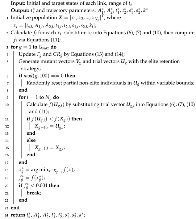
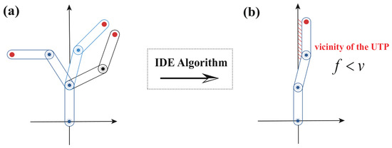
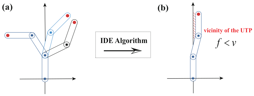
To efficiently obtain the trajectory parameters and controller switching time $t_s$ that satisfy the control objective, the IDE algorithm is employed to ensure the convergence criterion $f<v$ is fulfilled, as detailed in Algorithm 1. The effectiveness of the parameter optimization is shown in Figure 3.

Figure 3. IDE (Improved Differential Evolution) Algorithm Optimization Effect on Trajectory. (a) Without an IDE, the system is unable to swing from DIP to the vicinity of UTP. (b) After optimizing trajectory parameters via IDE, $f<v$ is achieved; links reach the vicinity of UTP simultaneously.

Based on the DE algorithm, the IDE algorithm incorporates an elite retention strategy that selects the top 10% of individuals in the population to directly advance to the next generation without undergoing mutation operations. Additionally, a dynamic adaptive adjustment mechanism for the mutation factor $F_g$ and crossover factor $C{R}_g$ is implemented:

$$F_g=\left\{\begin{array}{cc}1.2F_0,\hfill & {\eta }_g<0.3\hfill \\ 0.9F_0,\hfill & 0.3\le {\eta }_g<0.7\hfill \\ 0.7F_0,\hfill & {\eta }_g\ge 0.7\hfill \end{array}\right.$$

(13)

$$C{R}_g=min\left\{0.95,c{r}_0+0.05·\mathrm{rand}(0,1)\right\}$$

(14)

where ${\eta }_g$ denotes the iteration progress of the algorithm, $F_0$ and $c{r}_0$ are the initial values of the factors, and rand $(0,1)$ represents a random number generated in the range of 0 to 1.

Algorithm 1: IDE Algorithm for Trajectory Parameter Optimization

4. Tracking Controller Design

When $0\le t\le t_s$, to achieve tracking of the planned trajectory for the APP manipulator, this section designs a tracking controller based on the NFTSM. The core of this controller is the design of a non-singular sliding mode surface with fast convergence properties, combined with the continuous boundary layer method is incorporated to effectively suppress the state fluctuations caused by controller switching.

The position tracking error Equation (15a) and the velocity tracking error Equation (15b) of the active link are defined as follows:

$$\left\{\begin{array}{}\mathrm{(15a)}& e=q_1-{\overline{q}}_1,\mathrm{(15b)}& \dot{e}={\dot{q}}_1-{\dot{\overline{q}}}_1\end{array}\right.$$

By differentiating the expression in Equation (15b) and then substituting Equation (4b), we obtain:

$$\ddot{e}={\ddot{q}}_1-{\ddot{\overline{q}}}_1=F+B\tau -{\ddot{\overline{q}}}_1$$

(16)

The NFTSM surface is defined as follows:

$$s=e+\alpha {\left|e\right|}^{r_1}·\mathrm{sign}\left(e\right)+\beta {\left|\dot{e}\right|}^{r_2}·\mathrm{sign}\left(\dot{e}\right)$$

(17)

where $\alpha >0,\beta >0,1<r_2<2,r_1>r_2$.

The result after differentiation is:

$$\dot{s}=\dot{e}+\alpha r_1{\left|e\right|}^{r_1-1}\dot{e}·\mathrm{sign}\left(e\right)+\beta r_2{\left|\dot{e}\right|}^{r_2-1}·\mathrm{sign}\left(\dot{e}\right)\left(F+B\tau -{\ddot{\overline{q}}}_1\right)$$

(18)

Define reaching law is:

$$\dot{s}=-ks-\epsilon ·\mathrm{sign}\left(s\right)$$

(19)

Integrated Equations (18) and (19), the controller is obtained as follows:

$$\begin{array}{c}\hfill \tau =-{\displaystyle \frac{1}{B}}\left(F-{\ddot{\overline{q}}}_1+ks+\epsilon ·\mathrm{sign}\left(s\right)·{\displaystyle \frac{1+\alpha r_1{\left|e\right|}^{r_1-1}·\mathrm{sign}\left(e\right)}{\beta r_2{\left|\dot{e}\right|}^{r_2-2}·\mathrm{sign}\left(\dot{e}\right)}}\right)\end{array}$$

(20)

The description of each parameter is presented in Table 1. The sliding mode designed in this paper has the following two characteristics:

Table 1. Parameters of the NFTSMC.

Symbol	Description
$\alpha$	Linear term gain
$\beta$	Nonlinear term gain
$r_1$	Position error exponent
$r_2$	Velocity error exponent
k	Sliding gain
$\epsilon$	Reaching gain
$\delta$	Boundary layer thickness

(1)

Non-singularity: The condition $1<r_2<r_1<2$ guarantees that the denominator of Equation (20) is non-zero, thereby effectively avoiding the singularity problem.

(2)

Fast Convergence: Far from equilibrium, the $|\dot{e}{|}^{r_2}$ term dominates, providing stronger convergence acceleration than linear terms and rapidly driving the state toward the sliding surface. Near equilibrium, the ${\left|e\right|}^{r_1}$ term dominates, enabling fast adjustment along $s\approx 0$.

To weaken state fluctuations, a boundary layer is designed using a saturation function $\mathrm{sat}\left(s\right)$, which replaces the sign function $\mathrm{sign}\left(s\right)$ in the controller. The expression of $\mathrm{sat}\left(s\right)$ is given as follows:

$$\mathrm{sat}\left(s\right)=\left\{\begin{array}{cc}1\hfill & s>\delta \hfill \\ s/\delta \hfill & \left|s\right|\le \delta \hfill \\ -1\hfill & s<-\delta \hfill \end{array}\right.$$

(21)

where $0.001<\delta <0.05$. After replacing, the NFTSM controller (NFTSMC) is obtained as follows:

$$\begin{array}{cc}\hfill \tau =& -{\displaystyle \frac{1}{B}}\left(F-{\ddot{\overline{q}}}_1+ks+\epsilon ·\mathrm{sat}\left(s\right)·{\displaystyle \frac{\left(1+\alpha r_1·\mathrm{sat}\left(e\right)\right|{e|}^{r_1-1}·\mathrm{sat}\left(\dot{e}\right){\left|\dot{e}\right|}^{2-r_2}}{\beta r_2}}\right)\hfill \end{array}$$

(22)

In contrast to the traditional sliding mode controller (SMC) described in [23], the control law is given by:

$${\tau }_{\mathrm{SMC}}=-{\displaystyle \frac{1}{B}}\left(F-{\ddot{\overline{q}}}_1+{\epsilon }_1\dot{e}+{\epsilon }_2{s}_r+{\epsilon }_3·\mathrm{sign}\left(s_r\right)\right)$$

(23)

The NFTSMC not only maintains the properties of fast convergence and non-singularity, but also effectively suppresses state fluctuations at the moment of controller switching. The effectiveness of fluctuations suppression will be verified in Section 6.

Define a Lyapunov function as follows:

$$V={\displaystyle \frac{1}{2}}{s}^2$$

(24)

Differentiating Equation (24) and substituting Equation (19) into it yields:

$$\dot{V}=s\dot{s}=-k{s}^2-\epsilon ·\left|s\right|\le 0$$

(25)

According to LaSalle’s Invariance Principle, when $\dot{V}\equiv 0,s\equiv 0$, $q_1-{\overline{q}}_1\to 0$ and ${\dot{q}}_1-{\dot{\overline{q}}}_1\to 0$. Under this condition, the active link converges asymptotically to the target state along the optimized trajectory.

5. Stabilizing Controller Design

When $t>t_s$, the APP manipulator has reached the vicinity of the UTP and therefore requires immediate stabilization at the UTP. Due to the continuous effect of gravity, a standalone NFTSMC cannot stabilize the manipulator at the UTP. However, the system dynamics in the vicinity of the target position can be approximated by a linear model. Thus, we adopt the LQR method to design a stabilizing controller, achieving stable regulation of the manipulator at the target position.

The design of the stabilizing controller is based on the linearized system model at the UTP:

$$\dot{x}=Ax+B\tau$$

(26)

where A is the system matrix, and B is the input matrix corresponding to the control input of the active link. Define the LQR performance index to balance state deviation and control effort:

$$\mathrm{\Psi }={\int }_0^{\infty }\left[x^{T}Rx+Q{\tau }^2\right]dt$$

(27)

where the positive-definite matrix R restricts the state deviation from the target position, and the positive-semidefinite matrix Q penalizes the magnitude of the control input $\tau$. According to optimal control theory, the stabilizing controller that minimizes $\mathrm{\Psi }$ takes the state-feedback form:

$$\tau =-Kx$$

(28)

where the gain vector K is derived from the symmetric positive-definite solution W of the algebraic Riccati equation:

$$A^{T}W+WA-WB{Q}^{-1}{B}^{T}W+R=0$$

(29)

specifically, $K=Q^{-1}{B}^{T}W$.

Given Q and R, K can be obtained by solving the Riccati equation. Substituting Equation (28) into the linear system yields stable closed-loop dynamics, thus maintaining the stability of the manipulator at the target position.

6. Simulation Results

In this section, simulation experiments are conducted by setting $t_s$ within three intervals: $[2.0,2.5]$,$[2.5,3.0]$, and $[3.0,3.5]$. Experiments are performed to verify the effectiveness of the proposed control strategy. Additionally, the fluctuation suppression performance of NFTSMC and SMC is compared during controller switching, so as to further verify the effectiveness of the proposed controller.

6.1. Case 1

The structure parameters of the APP manipulator are taken from [33] and given in Table 2.

Table 2. Structure parameters.

Link i	${\mathit{m}}_{\mathit{i}}$ (kg)	${\mathit{L}}_{\mathit{i}}$ (m)	${\mathit{l}}_{\mathit{i}}$ (m)	${\mathit{J}}_{\mathit{i}}$ (kg·m2)
1	1.258	0.340	0.170	0.0121
2	5.686	0.290	0.145	0.0398
3	2.162	0.520	0.260	0.0487

The initial state is set to $[-\pi ,0,0,0,0,0]$, and the target state set to $[0,-2\pi ,2\pi ,0,0,0]$. The parameter settings of the IDE algorithm used in this paper are as follows:

$$\left\{\begin{array}{c}{N}_p=50,G_{\max }=500,\hfill \\ F_0=0.5,c{r}_0=0.75\hfill \end{array}\right.$$

(30)

By setting $t_s\in [2.0,2.5]$, combined with Table 2, the trajectory parameters obtained after optimization using the IDE algorithm are as follows:

$$\left\{\begin{array}{c}{t}_s=2.2465,k=4.9401,A_1=-2.4844,A_2=1.7705,\hfill \\ t_1=0.3206,t_2=0.9612,s_1=0.0673,s_2=0.1735,\hfill \end{array}\right.$$

(31)

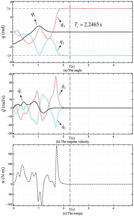
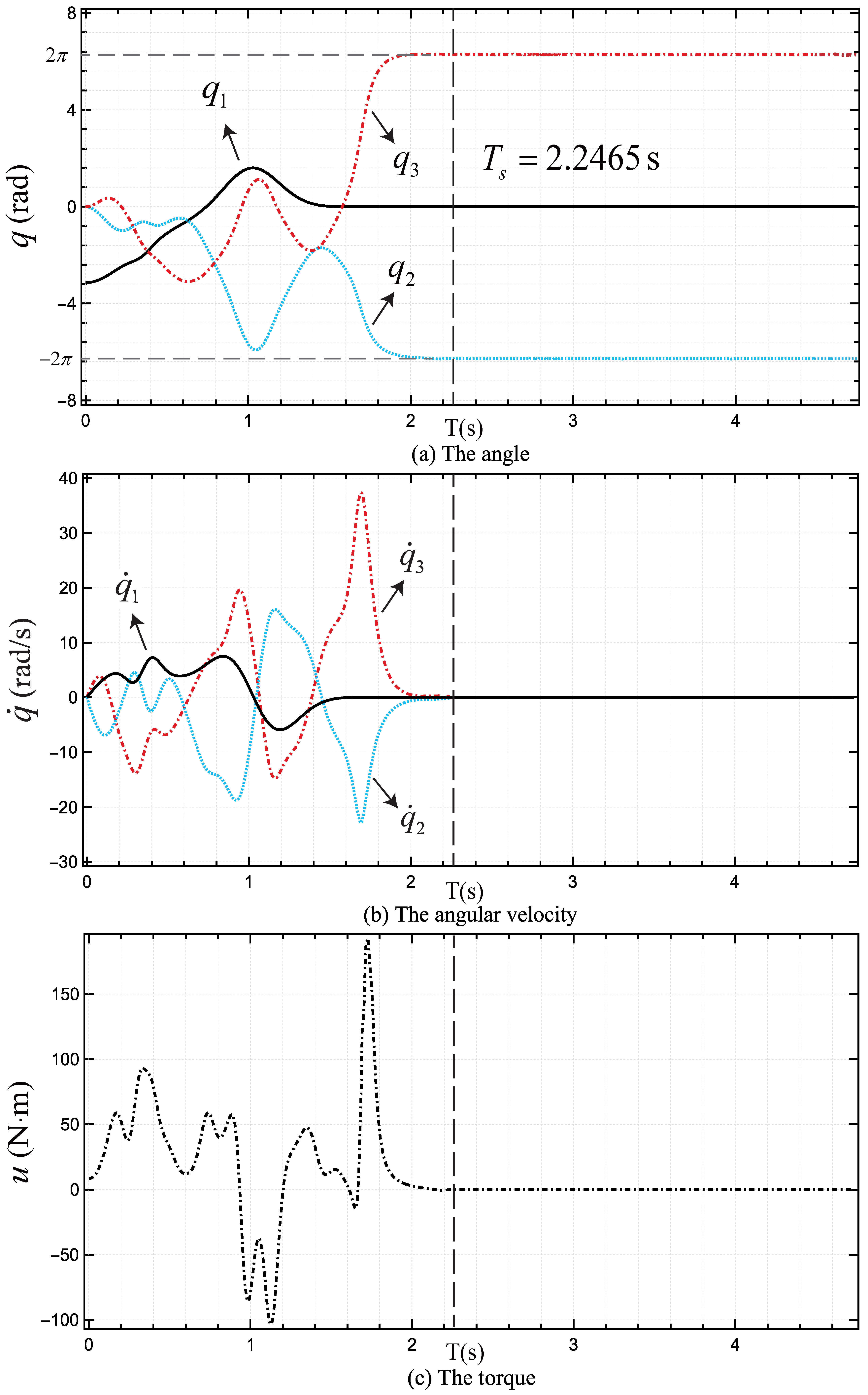
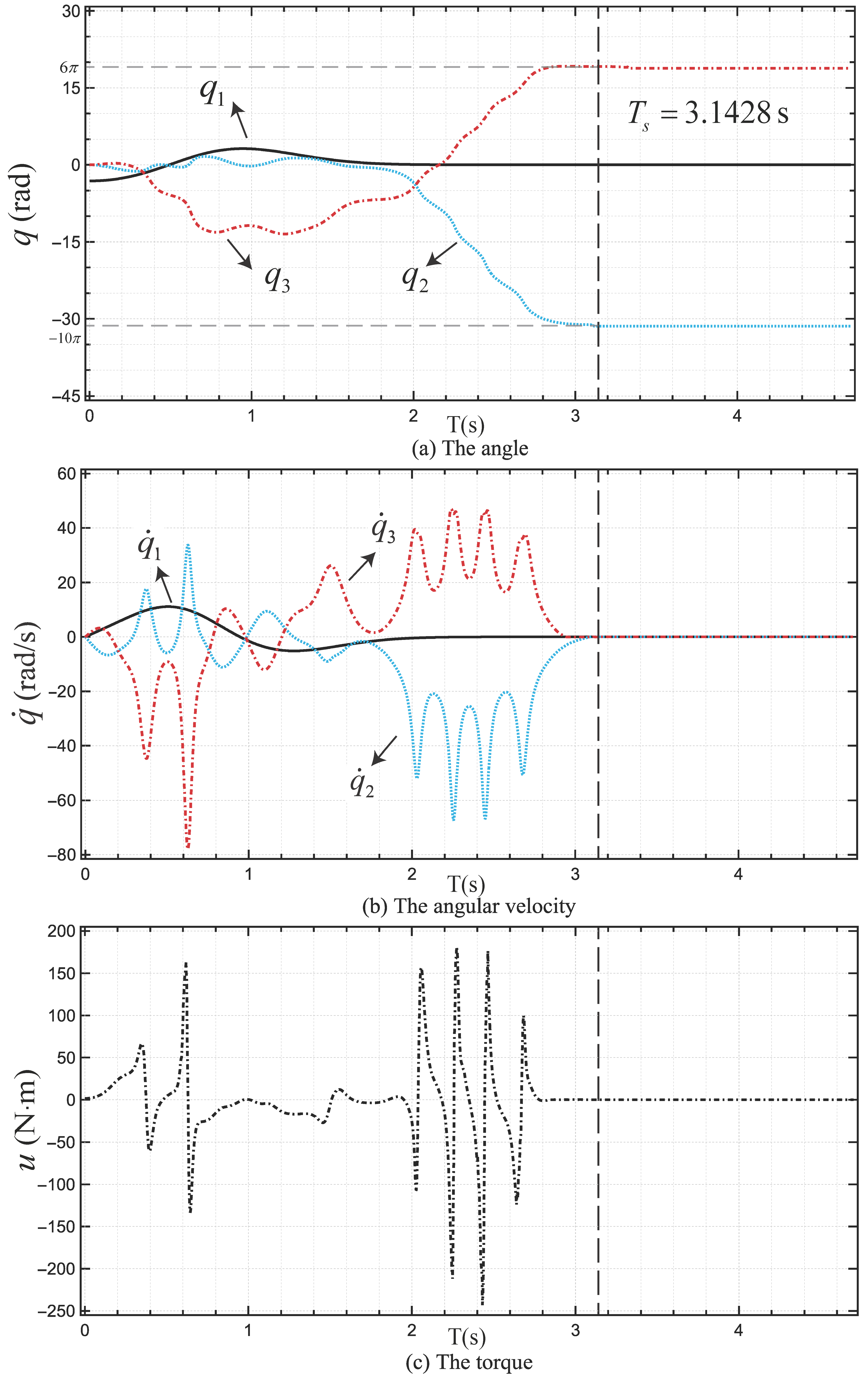
The simulation results in Figure 4 demonstrate that when $t<2.2465$ s, the links gradually swing up from the DIP to the vicinity of the UTP under the tracking controller Equation (22). During this process, the maximum value of torque is approximately 186 N·m, which lies within a reasonable range. At $t=2.2465$ s, the controller smoothly switches from the tracking controller Equation (22) to the stabilizing controller Equation (28). This switching causes no state mutations and does not disrupt the system’s convergence trend. After entering the phase of $t>2.246$ s, the joint angles of all links remain stable at $[0,-2\pi ,2\pi ]$, the angular velocities and torques converge steadily to $[0,0,0]$, the end-effector is stabilized at the UTP by the stabilizing controller Equation (28).

Figure 4. Simulation results of $t_s\in [2.0,2.5]$ s.

6.2. Case 2

To further verify the effectiveness of the proposed method, the initial state is set to $[-\pi ,0,0,0,0,0]$ and the target state set to $[0,0,0,0,0,0]$. The parameters of the IDE algorithm are kept consistent with Equation (30).

With $t_s\in [2.5,3.0]$ set as a constraint, in combination with Table 2, the trajectory parameters obtained by the optimization of the IDE algorithm are as follows:

$$\left\{\begin{array}{c}{t}_s=2.8600,k=4.5037,A_1=-6.8000,A_2=7.5151,\hfill \\ t_1=0.0703,t_2=0.6026,s_1=0.2320,s_2=0.4164,\hfill \end{array}\right.$$

(32)

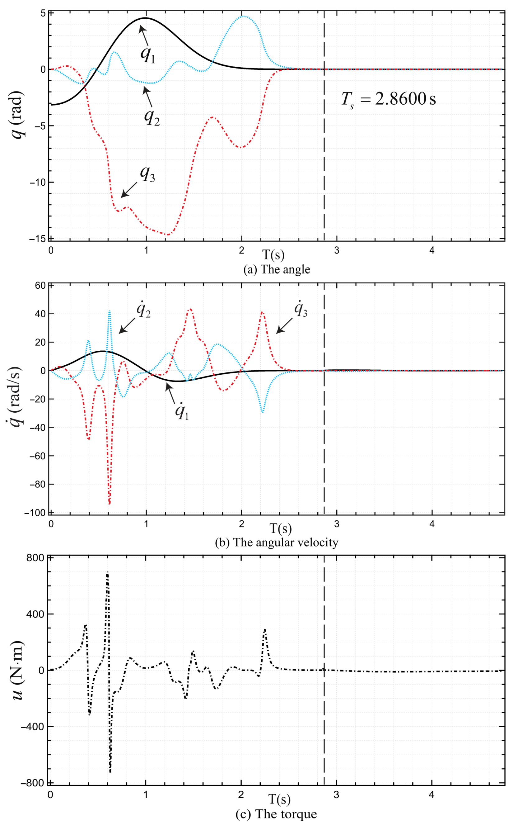
As shown in Figure 5, with the tracking controller Equation (22), all links are swung up from the DIP to approach the vicinity of the UTP when $t<2.86$ s. However, during $t<0.95$ s, the control torque applied to the joints remains relatively large, as shown in Figure 5c. Abrupt angular velocity variation results in large angular accelerations, thus requiring a larger torque. When the switching time of $t=2.86$ s is reached, the controller is switched from the tracking controller Equation (22) to the stabilizing controller Equation (28). Since the $f<0.001$ at this moment, the states of all links have been close to the final steady state. Thus, this switching does not disrupt the convergent behavior of the joint angles, angular velocities, or torques. When $t>2.86$ s, the system approaches a steady state, all joint angles remain at $[0,0,0]$, the torque applied to the first joint, and the angular velocities of all joints converge to zero. The system is ultimately stabilized at the UTP.

Figure 5. Simulation results of $t_s\in [2.5,3.0]$ s.

6.3. Case 3

In this case, the target state of the system is set as $[0,-10\pi ,6\pi ]$, while the initial state and parameters of the IDE algorithm remain unchanged. For $t_s\in [3.0,3.5]$, the trajectory parameters obtained after optimization are listed below:

$$\left\{\begin{array}{c}{t}_s=3.1428,k=4.2905,A_1=-5.6340,A_2=7.5830,\hfill \\ t_1=0.0052,t_2=0.4340,s_1=0.3161,s_2=0.4480,\hfill \end{array}\right.$$

(33)

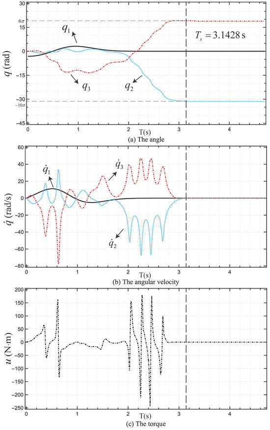
As shown in Figure 6, when $t_s<3.1428$ s, links are swung up under the tracking controller Equation (22). When $t_s =3.1428$ s, the controller switching is completed. It can be observed from Figure 6c that no abrupt torque variation occurs at the controller switching instant, thus achieving a smoother transition. After $t_s >3.1428$ s, the system reaches the target states, where the steady-state values of the joint angles are $[0,-10\pi ,6\pi ]$ rad, and the steady-state values of angular velocities and torques are sufficiently close to zero. The proposed method effectively avoids the difficulty of balancing region division as well as the singularity problem; the system can be directly swung up to the vicinity of the UTP within a prescribed time.

Figure 6. Simulation results of $t_s\in [3.0,3.5]$ s.

6.4. Controller Performance Verification

6.4.1. Fluctuation Suppression Performance

To clearly demonstrate the state fluctuation suppression performance of the NFTSMC at the controller switching moment, we obtain a set of trajectory parameters satisfying $f<0.06$ within the range of $t_s\in [2.5,3.0]$. The optimized trajectory parameters are given as follows:

$$\left\{\begin{array}{c}{t}_s=2.8728,k=4.4983,A_1=-6.7954,A_2=7.5191,\hfill \\ t_1=0.0705,t_2=0.6025,s_1=0.2321,s_2=0.4162\hfill \end{array}\right.$$

(34)

In this case, since f is relatively large, a deviation exists when the links move to the vicinity of the UTP at $t_s$, leading to fluctuations in the joint angles.

For the NFTSMC in Equation (22), the parameters are as follows:

$$\left\{\begin{array}{c}k=18,\epsilon =10,\alpha =12,\beta =8,\hfill \\ r_1=1.6,r_2=1.1,\delta =0.01\hfill \end{array}\right.$$

(35)

For the SMC in Equation (23), the parameters from [23] are used as follows:

$${\epsilon }_1=1.2,{\epsilon }_2=1.0,{\epsilon }_3=0.1,$$

(36)

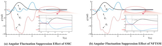
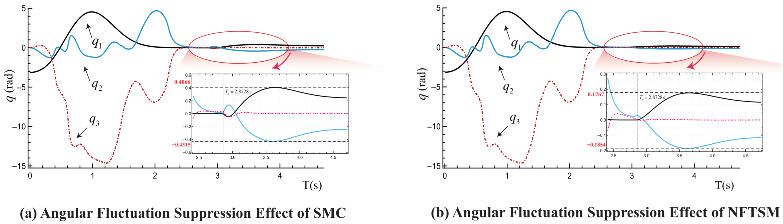
As shown in Figure 7, at the controller switching instants, the sign function in SMC causes obvious angular fluctuation. In contrast, NFTSMC yields smaller angular fluctuations under the same structural parameters and simulation conditions.

Figure 7. Angle Fluctuations for SMC and NFTSMC at $t_s$.

The data of angular fluctuations in Figure 7 are collected and summarized in Table 3. Based on the statistical results in Table 3, the absolute angular fluctuation amplitude of the SMC can be calculated. The specific calculation formula is given as follows:

$$\eta ={\displaystyle \frac{{\delta }_{\mathrm{SMC}}-{\delta }_{\mathrm{NFTSMC}}}{{\delta }_{\mathrm{SMC}}}}\times 100\%=56.8\%$$

(37)

Table 3. Comparison of angular fluctuation amplitude.

Maximum Peak ${\mathit{\theta }}_{\mathbf{max}}$ (rad)	Minimum Trough ${\mathit{\theta }}_{\mathbf{min}}$ (rad)	Amplitude Difference $\mathit{\delta }={\mathit{\theta }}_{\mathbf{max}}-{\mathit{\theta }}_{\mathbf{min}}$ (rad)
0.1767	−0.1854	0.3621
0.4066	−0.4315	0.8381

According to the absolute angular fluctuation amplitude, the NFTSMC can suppress fluctuations at the controller switching moment. Specifically, the NFTSMC’s angular fluctuation suppression effect is improved by more than 50% compared to that of the SMC.

6.4.2. Robust Performance

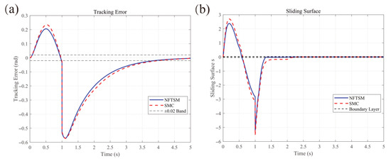
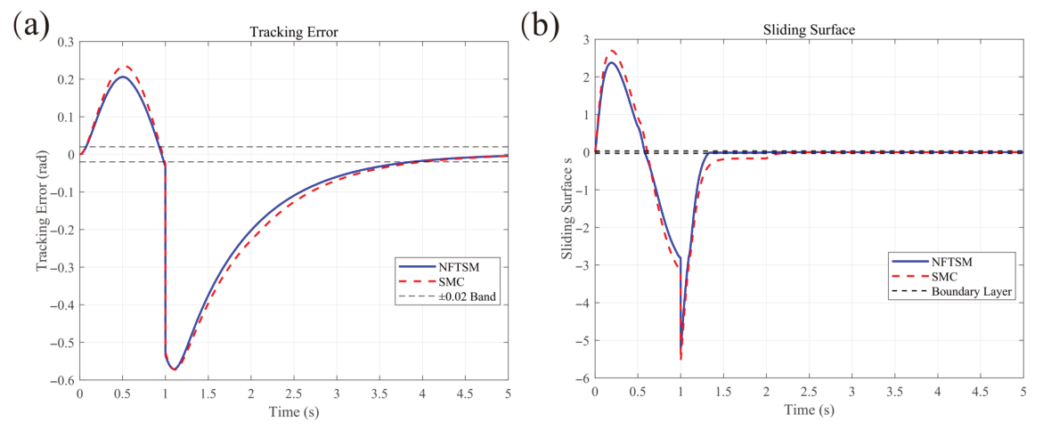
To verify the robustness of the NFTSMC, a step disturbance $d\left(t\right)$ with an amplitude of 0.5 is applied for $t\in [1.0,2.0]$ s. The results are shown in Figure 8.

Figure 8. Tracking Error and Sliding Surface Variation for NFTSM and SMC under Disturbance. (a) Tracking error comparison; (b) Sliding surface variation.

Figure 8a shows that the NFTSMC achieves a lower peak error and a shorter recovery time compared with the SMC. Figure 8b further demonstrates that under the disturbance, the sliding surface of the SMC exhibits a large deviation, but the sliding surface of the NFTSMC maintains a smaller deviation. These results verify that the NFTSMC achieves superior tracking accuracy and robustness compared to the SMC.

7. Conclusions

This paper proposed an asymptotic stabilization control method based on trajectory optimization for APP manipulators, achieving the swing-up and stabilization control of the system. First, the dynamic model of the APP manipulator was established, and a trajectory from the DIP to the UTP was planned for the active link. Then, based on the trajectory and the coupling relationship between links, the IDE algorithm was employed to optimize the trajectory parameters within a prescribed time range, such that all links could reach the vicinity of the UTP simultaneously. On this basis, a controller switching scheme was introduced to achieve the control objective. In the swing-up phase, a tracking controller based on NFTSM was designed to swing the active link along the optimized trajectory. After the system approached the vicinity of the UTP, an LQR-based stabilization controller was further applied to stabilize the system at the UTP. Finally, the controller switching time was set within $[2.0,3.5]$ s in the simulations, verifying the effectiveness of the proposed method.

Results demonstrated that the proposed method achieved faster swing-up and stabilization compared to the energy-based control, avoiding region division and simplifying switching conditions. Comparative simulations between NFTSMC and SMC showed that the controller effectively suppressed state fluctuations during switching and provided smoother stabilization.

In fact, the trajectory design proposed in this paper is independent of the system’s structural parameters, relying solely on the initial and target states of links. Therefore, changes in the system’s structural parameters do not affect the trajectory design, demonstrating the universality of the proposed method. Additionally, the proposed method avoids the difficulty of balancing region division, and the designed time-switching condition is more easily satisfied than the state-switching condition. The designed controller effectively suppresses state fluctuations and avoids singularity. In practical scenarios, the system may be affected by many factors, such as chaos, modeling uncertainties, and external disturbances [34]. Therefore, the overall robustness of the method still needs to be further improved. In future work, we will set up experimental platforms to further verify the effectiveness of the proposed method and improve the control strategy.

References

- Reyhanoglu, M.; van der Schaft, A.; McClamroch, N.H.; Kolmanovsky, I. Dynamics and control of a class of underactuated mechanical systems. IEEE Trans. Autom. Control 2002, 44, 1663–1671. [Google Scholar] [CrossRef] [Scilit]
- Zhang, X.; Zhou, Z.; Shi, Y.; Li, M.; Peng, W.; Song, C.; Li, Z.; Cheng, X.; Zhang, M. Adaptive sliding mode control for underactuated ship-mounted cranes with dead zones and actuated/unactuated state constraints. Ocean Eng. 2025, 340, 122275. [Google Scholar] [CrossRef] [Scilit]
- Zhao, T.; Sun, M.; Wang, S.; Han, G.; Wang, H.; Chen, H.; Sun, Y. Dynamic analysis and robust control of ship-mounted crane with multi-cable anti-swing system. Ocean Eng. 2024, 291, 116376. [Google Scholar] [CrossRef] [Scilit]
- Liu, W.; Zhang, X. Fault-tolerant trajectory tracking control for underactuated surface ships with input saturation and dead-zone constraints. Ocean Eng. 2025, 342, 122852. [Google Scholar] [CrossRef] [Scilit]
- Li, H.H.; Xing, W.B.; Jiao, H.; Yang, Z.L.; Li, Y. Deep bi-directional information-empowered ship trajectory prediction for maritime autonomous surface ships. Transp. Res. Part E Logist. Transp. Rev. 2024, 181, 103367. [Google Scholar] [CrossRef] [Scilit]
- Yaman, Y.; Arslan, B.; Ergin, Ö.Ç.; Aukes, D.M.; Özcan, O. Maneuverable Multilegged Locomotion through Anisotropically Arranged Soft Backbones in a Single-Actuator Modular Miniature Robot. Adv. Intell. Syst. 2026, e202501252. [Google Scholar] [CrossRef] [Scilit]
- Jeyabalan, P.K.M.; Thiagu, S.; Nehrujee, A.; Sujatha, S.; Balasubramanian, S. Motorized Arm Support (MARS)—An Underactuated Robot for Adaptive Arm De-weighting in Neurorehabilitation. IEEE Access 2026, 14, 23244–23256. [Google Scholar] [CrossRef] [Scilit]
- Liu, Y.; Yu, H.N. A survey of underactuated mechanical systems. IET Control Theory Appl. 2013, 7, 921–935. [Google Scholar] [CrossRef] [Scilit]
- Spong, M.W. Underactuated mechanical systems. In Control Problems in Robotics and Automation; Springer: Berlin/Heidelberg, Germany, 2005; pp. 135–150. [Google Scholar]
- Lai, X.Z.; Zhang, A.C.; Wu, M.; She, J.H. Singularity-avoiding swing-up control for underactuated three-link gymnast robot using virtual coupling between control torques. Int. J. Robust Nonlinear Control 2015, 25, 207–221. [Google Scholar] [CrossRef] [Scilit]
- Hernández-Guzmán, V.M.; Silva-Ortigoza, R.; Orrante-Sakanassi, J.A. Control of Pendubot. In Automatic Control with Experiments; Springer: Berlin/Heidelberg, Germany, 2024; pp. 725–771. [Google Scholar]
- Gulan, M.; Salaj, M.; Rohal’-Ilkiv, B. Tracking Control of Unforced and Forced Equilibrium Positions of the Pendubot System: A Nonlinear MHE and MPC Approach. Actuators 2023, 12, 343. [Google Scholar] [CrossRef] [Scilit]
- Xin, X.; Ji, X.H.; Wang, Z.Y.; Liu, Y.N. Strongly stabilizing the Acrobot by optimizing maximal relative stability via observation point selection. Automatica 2026, 185, 112814. [Google Scholar] [CrossRef] [Scilit]
- Lai, X.Z.; Pan, C.Z.; Wu, M.; Yang, S.X. Unified control of n-link underactuated manipulator with single passive joint: A reduced order approach. Mech. Mach. Theory 2012, 56, 170–185. [Google Scholar] [CrossRef] [Scilit]
- Albahkali, T.; Mukherjee, R.; Das, T. Swing-up control of the pendubot: An impulse–momentum approach. IEEE Trans. Robot. 2009, 25, 975–982. [Google Scholar] [CrossRef] [Scilit]
- Lai, X.; Zhang, Z.; Wu, M. Energy decoupling control strategy for three-link underactuated manipulator. Acta Autom. Sin. 2011, 37, 67–73. [Google Scholar] [CrossRef] [Scilit]
- Liu, Y.N.; Xin, X. Global motion analysis of energy-based control for 3-link planar robot with a single actuator at the first joint. Nonlinear Dyn. 2017, 88, 1749–1768. [Google Scholar] [CrossRef] [Scilit]
- Azimi, M.M.; Koofigar, H.R. Adaptive fuzzy backstepping controller design for uncertain underactuated robotic systems. Nonlinear Dyn. 2015, 79, 1457–1468. [Google Scholar] [CrossRef] [Scilit]
- Lai, X.Z.; Zhang, A.C.; She, J.H.; Wu, M. Motion control of underactuated three-link gymnast robot based on combination of energy and posture. IET Control Theory Appl. 2011, 5, 1484–1493. [Google Scholar] [CrossRef] [Scilit]
- Nath, V.; Mitra, R. Swing-up and control of Rotary Inverted Pendulum using pole placement with integrator. In 2014 Recent Advances in Engineering and Computational Sciences (RAECS); IEEE: Piscataway, NJ, USA, 2014; pp. 1–5. [Google Scholar]
- Tran, T.B.; Nguyen, H.T.; Nguyen, T.; Dang, D.D.; Pham, D.M.Q.; Le, N.D.; Huynh, H.K.; Nguyen, B.H.; Nguyen, N.H.T.; Pham, L.Q.T.; et al. Trajectory tracking using LQR control for Pendubot: Simulation and experiment. J. Fuzzy Syst. Control 2024, 2, 18–21. [Google Scholar] [CrossRef] [Scilit]
- Wang, L.J.; Lai, X.Z.; Zhang, P.; Wu, M. Motion Control Strategy Based on Integrated Trajectory for the Pendubot. In 2021 European Control Conference (ECC); IEEE: Piscataway, NJ, USA, 2021; pp. 2151–2156. [Google Scholar]
- Wang, L.J.; Lai, X.Z.; Meng, Q.X.; Wu, M. Effective control method based on trajectory optimization for three-link vertical underactuated manipulators with only one active joint. IEEE Trans. Cybern. 2021, 53, 3782–3793. [Google Scholar] [CrossRef] [Scilit]
- Tran, M.D.; Le, D.T.D.; Phan, H.P.; Vo, H.V.; Ngo, D.Q.T.; Nguyen, N.D.; Nguyen, T.P.; Tran, N.L.; Vo, T.A.; Le, T.T.H. Analysis of Linear and Intelligent Control for Balancing Pendubot System. J. Fuzzy Syst. Control 2024, 3, 16–21. [Google Scholar] [CrossRef] [Scilit]
- Van Heerden, K.; Fujimoto, Y.; Kawamura, A. A combination of particle swarm optimization and model predictive control on graphics hardware for real-time trajectory planning of the under-actuated nonlinear Acrobot. In 2014 IEEE 13th International Workshop on Advanced Motion Control (AMC); IEEE: Piscataway, NJ, USA, 2014; pp. 464–469. [Google Scholar]
- Cheng, H.T.; Chen, H.P.; Gao, B.T.; Zhang, X.H. General swing-up methodology for the vertical three-link underactuated manipulator. In 2013 IEEE International Conference on Cyber Technology in Automation, Control and Intelligent Systems; IEEE: Piscataway, NJ, USA, 2013; pp. 379–384. [Google Scholar]
- Mu, C.; He, H. Dynamic behavior of terminal sliding mode control. IEEE Trans. Ind. Electron. 2017, 65, 3480–3490. [Google Scholar] [CrossRef] [Scilit]
- Feng, Q.; Zhang, A.; Zhang, X.; Pang, G.; Liu, Z. Robust Stabilization of Underactuated TORA System Based on Disturbance Observer and Fixed-Time Sliding Mode Control Method. Actuators 2022, 11, 271. [Google Scholar] [CrossRef] [Scilit]
- Wang, X.; Liu, Y.; Xue, G.; Bai, F.; Huang, S. A super-twisting non-singular terminal sliding mode control strategy based on particle swarm optimization for underwater two-link manipulator trajectory tracking. Ocean Eng. 2026, 352, 124581. [Google Scholar] [CrossRef] [Scilit]
- Feng, Y.; Yu, X.H.; Man, Z.H. Non-singular terminal sliding mode control of rigid manipulators. Automatica 2002, 38, 2159–2167. [Google Scholar] [CrossRef] [Scilit]
- Zhao, J.; Dang, R.; Zhu, B.; Chen, Z.; Han, J.; Zhang, P.; Song, D.; Jia, S. Disturbance-rejection pressure control for integrated brake system based on improved non-singular fast terminal sliding mode. Control Eng. Pract. 2026, 170, 106811. [Google Scholar] [CrossRef] [Scilit]
- Wang, Y.C.; Chen, H.J.; Zhang, M.L.; Chen, B.B.; Jia, R.S.; Mao, J.F. Non-singular fast terminal sliding mode control of PMSMs with disturbance compensation. J. Power Electron. 2025, 25, 1245–1255. [Google Scholar] [CrossRef] [Scilit]
- Wang, L.J.; Lai, X.Z.; Zhang, P.; Wu, M. Single controller design based on integrated trajectory for three-link vertical underactuated manipulators with first active joint. Int. J. Control 2023, 96, 424–434. [Google Scholar] [CrossRef] [Scilit]
- Ravishankar, A.; Ghosal, A. Nonlinear dynamics and chaotic motions in feedback-controlled two-and three-degree-of-freedom robots. Int. J. Robot. Res. 1999, 18, 93–108. [Google Scholar] [CrossRef] [Scilit]
Disclaimer/Publisher’s Note: The statements, opinions and data contained in all publications are solely those of the individual author(s) and contributor(s) and not of MDPI and/or the editor(s). MDPI and/or the editor(s) disclaim responsibility for any injury to people or property resulting from any ideas, methods, instructions or products referred to in the content. |
© 2026 by the authors. Licensee MDPI, Basel, Switzerland. This article is an open access article distributed under the terms and conditions of the Creative Commons Attribution (CC BY) license.