Real-Time HILS Comparison of Full-State Feedback and LQ-Servo Tracking Control for a Wheeled Bipedal Robot

Abstract

Wheeled bipedal robots are promising for industrial mobility because they combine tight turning, agile balancing, and efficient rolling. Their inherently unstable and underactuated dynamics make reliable reference tracking challenging, particularly in the presence of sustained external disturbances and modeling errors. This paper presents a systematic modeling and control study using a three-degrees-of-freedom sagittal plane representation derived from the original six-degrees-of-freedom dynamics. Two linear tracking controllers are designed and compared: a full state feedback tracking controller and a linear quadratic servo controller with integral action. Practical performance is validated through real-time hardware in the loop simulation, where the controller runs on embedded hardware and the plant is executed on a real-time target including discrete time-sampling effects and analog input output communication noise associated with signal transmission. The results show that both controllers achieve stabilization, while the comparative HILS results reveal a trade-off rather than a uniformly superior controller. The full state feedback controller often yields lower finite-horizon position tracking errors, whereas the linear quadratic servo controller provides tighter body-pitch regulation and the more reliable removal of steady-state offset under sustained constant disturbances. These results demonstrate the feasibility of optimal servo control on cost-effective embedded platforms and indicate that controller selection should depend on the desired balance, considering tracking accuracy, disturbance rejection, convergence behavior, and actuator usage.

1. Introduction

Wheeled bipedal robots (WBRs) have emerged as compact and agile mobile platforms that combine the high-speed efficiency of wheeled locomotion with the posture-regulation capability of articulated legs [1]. By actively modulating the center of mass (CoM), WBRs can maintain dynamic balance while operating within confined industrial environments, making them promising candidates for logistics, inspection, and surveillance applications. However, the inherently unstable inverted-pendulum dynamics and underactuated structure of WBRs render their balance and trajectory tracking highly sensitive to actuator saturation, parameter uncertainty, and persistent disturbances such as ground inclinations and payload variations [2].

Ensuring both stable balance and accurate longitudinal tracking under sustained disturbances remains a central control challenge. While optimal state-feedback methods such as Linear Quadratic Regulator (LQR) have been widely adopted for WBR stabilization, their practical deployment often requires the explicit treatment of steady-state tracking errors and implementation constraints beyond idealized simulation environments [3,4,5,6]. Specifically, constant torque biases induced by slope or modeling mismatch may lead to residual offsets unless integral action is systematically incorporated into the control framework.

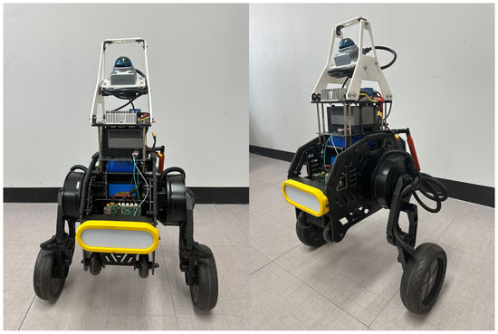
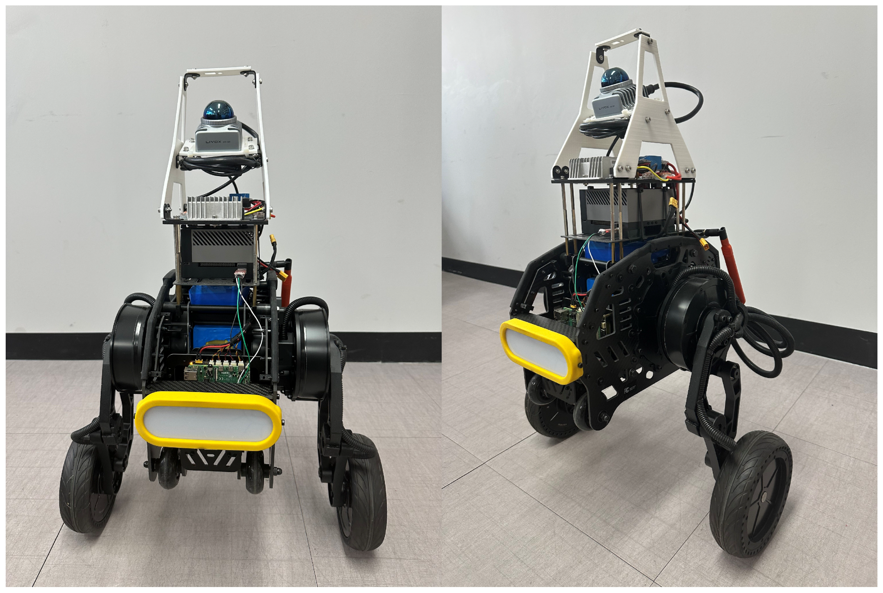
An example of the WBR platform considered in this study is shown in Figure 1.

Figure 1. Example WBR platform shown in front and oblique views.

Although integral augmentation is theoretically well established in optimal servo control formulations, its comparative evaluation against conventional full-state tracking strategies under identical design conditions has not been sufficiently investigated for embedded WBR platforms [1,3,5,7,8,9,10,11]. Moreover, many prior studies emphasize simulation-level validation, leaving a gap in implementation-level analysis that accounts for sampling effects, actuator nonlinearities, and measurement noise.

To address these issues, this paper investigates the practical realization of an integral-augmented optimal tracking strategy for a three-degrees-of-freedom sagittal-plane WBR model. A Linear Quadratic Servo (LQ-Servo) controller is systematically compared with a conventional Full-State Feedback (FSF) tracking controller under identical weighting structures. Both controllers are discretized and executed on embedded hardware within a real-time Hardware-in-the-Loop Simulation (HILS) framework, enabling implementation-level performance evaluation.

The main contributions of this work are summarized as follows:

• Development of a unified control-oriented 3-DOF sagittal-plane WBR model enabling structured comparison between FSF and LQ-Servo tracking controllers.
• Practical embedded realization of an integral-augmented optimal controller targeting steady-state error elimination under constant disturbance torque.
• Real-time HILS validation quantifying tracking accuracy and robustness through time-domain metrics and disk margin analysis.

This study provides practical guidance for selecting tracking architectures for cost-effective embedded WBR systems operating under sustained disturbances and parametric uncertainties.

2. Related Work and Positioning

2.1. WBR Platforms, Modeling, and Balance Control

WBRs combine wheeled locomotion efficiency with leg-assisted posture regulation and terrain adaptability. Recent surveys summarize the evolution of wheel-legged platforms and the breadth of modeling and control approaches reported for balancing and locomotion [1,10]. The related literature on two-wheeled self-balancing robots also provides useful context regarding inverted-pendulum-based modeling and practical stabilization issues that carry over to WBR formulations [12]. Representative modern hardware platforms, such as direct-drive multi-DoF WBRs, have further motivated control-oriented model simplifications suitable for real-time implementation and benchmarking [13].

On the control side, recent studies have reported dynamic whole-body locomotion and terrain-aware stabilization for WBRs using model-based planning and feedback control, typically emphasizing balance maintenance and maneuverability on uneven terrain [11,14]. While these works demonstrate improved mobility and stability, systematic discussion of longitudinal tracking robustness and steady-state offset under sustained disturbances is often secondary to balance regulation objectives [1,3,12].

2.2. LQR-Based and Hybrid Control Architectures

LQR-based state feedback remains a cornerstone for WBR stabilization due to its tractable design and performance around linearized operating points [15]. To improve robustness and disturbance rejection, several hybrid extensions have been explored. For example, LQR has been combined with Active Disturbance Rejection Control (ADRC) to mitigate environmental noise and unmodeled effects [4]. Other studies incorporate additional compensation terms or auxiliary loops around an LQR core, such as friction feedforward in LQR-based balancing for wheel-legged robots [16] and hybrid LQR–PD structures to address coupling effects and maintain implementable complexity [6]. Fuzzy LQR–PID schemes have also been proposed to handle uncertainty and operating-condition variability [17], while comparative studies between PID and LQR have been used to highlight performance trade-offs under disturbances [18].

In parallel, optimal output regulation and data-driven optimal control variants have been investigated to improve regulation and tracking under uncertainty [19]. Although these architectures enhance robustness, many introduce additional heuristic tuning layers or focus primarily on stabilization and disturbance attenuation, rather than a controlled comparison of tracking architectures with explicit steady-state offset elimination under identical optimal weighting conditions. From a robustness perspective, classical robust/optimal control theory provides the conceptual background for how nominal optimal controllers may lose margins under uncertainty and motivates margin-based evaluation beyond time-domain tracking indices [20]. Related position-tracking studies using conventional PID-based control have also been reported in other actuator systems, providing useful reference points for tracking-performance analysis [21].

2.3. Servo-Oriented Tracking and Offset Elimination

The elimination of steady-state tracking error under constant disturbances (e.g., slope-induced load torque) motivates servo-oriented formulations that augment the controller with integral action. Optimal servo concepts and integral augmentation are well established in the linear-quadratic framework [7,22]. In robotics-related balancing systems, Kim et al. [5] demonstrated that an LQ-Servo structure with reduced-order observation can achieve effective tracking performance while reducing sensing requirements. However, comparative studies that isolate the effect of integral augmentation by evaluating (i) conventional full-state tracking and (ii) integral-augmented LQ-Servo tracking under the same nominal modeling assumptions and cost structures remain limited, particularly for multi-DoF WBR configurations executed on embedded hardware.

2.4. Implementation-Level Validation via HILS

Hardware-in-the-Loop Simulation (HILS) has long been used to bridge numerical simulation and deployment by exposing controllers to realistic execution constraints, I/O, and plant-interface effects [23,24]. More recent overviews further emphasize engineering challenges and practical considerations for HIL/HILS workflows across domains [25]. In robotics and mechatronic control applications, HILS enables evaluation of sampling effects, actuator nonlinearities, and measurement noise before physical experimentation, supporting safer and more repeatable controller benchmarking [26,27].

In addition to time-domain metrics, robustness assessment using stability-margin concepts is increasingly used to complement tracking results. Disk margin analysis provides an implementation-relevant robustness indicator that can capture multiloop gain/phase uncertainty effects beyond classical SISO margins [28]. Practical deployment also requires consideration of actuator saturation and integral windup in servo-type designs; established anti-windup frameworks provide relevant background for mitigating such effects in implementations [29].

2.5. Positioning of This Work

In contrast to prior studies that primarily emphasize stabilization, hybrid heuristic extensions, or simulation-centered validation, this work focuses on a controlled comparison between (i) a conventional Full-State Feedback (FSF) tracking controller and (ii) an integral-augmented LQ-Servo controller, designed under identical optimal weighting structures. Both controllers are executed in discrete time on embedded hardware and evaluated within a real-time HILS environment, enabling implementation-level insight into steady-state tracking robustness and disturbance rejection. The study further complements time-domain tracking indices with disk margin analysis to connect tracking performance with robustness to uncertainty and implementation effects [28].

3. System Overview and Modeling

3.1. Robot Description and Coordinates

This study considers a 6-DoF WBR composed entirely of direct-drive joints. The original mechanical structure consists of two articulated legs, a body, and a pair of wheels for ground locomotion. To facilitate control-oriented modeling and a systematic comparison of tracking controllers, the multi-link leg structure is simplified into a single variable-length virtual leg [13].

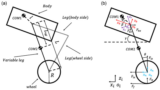
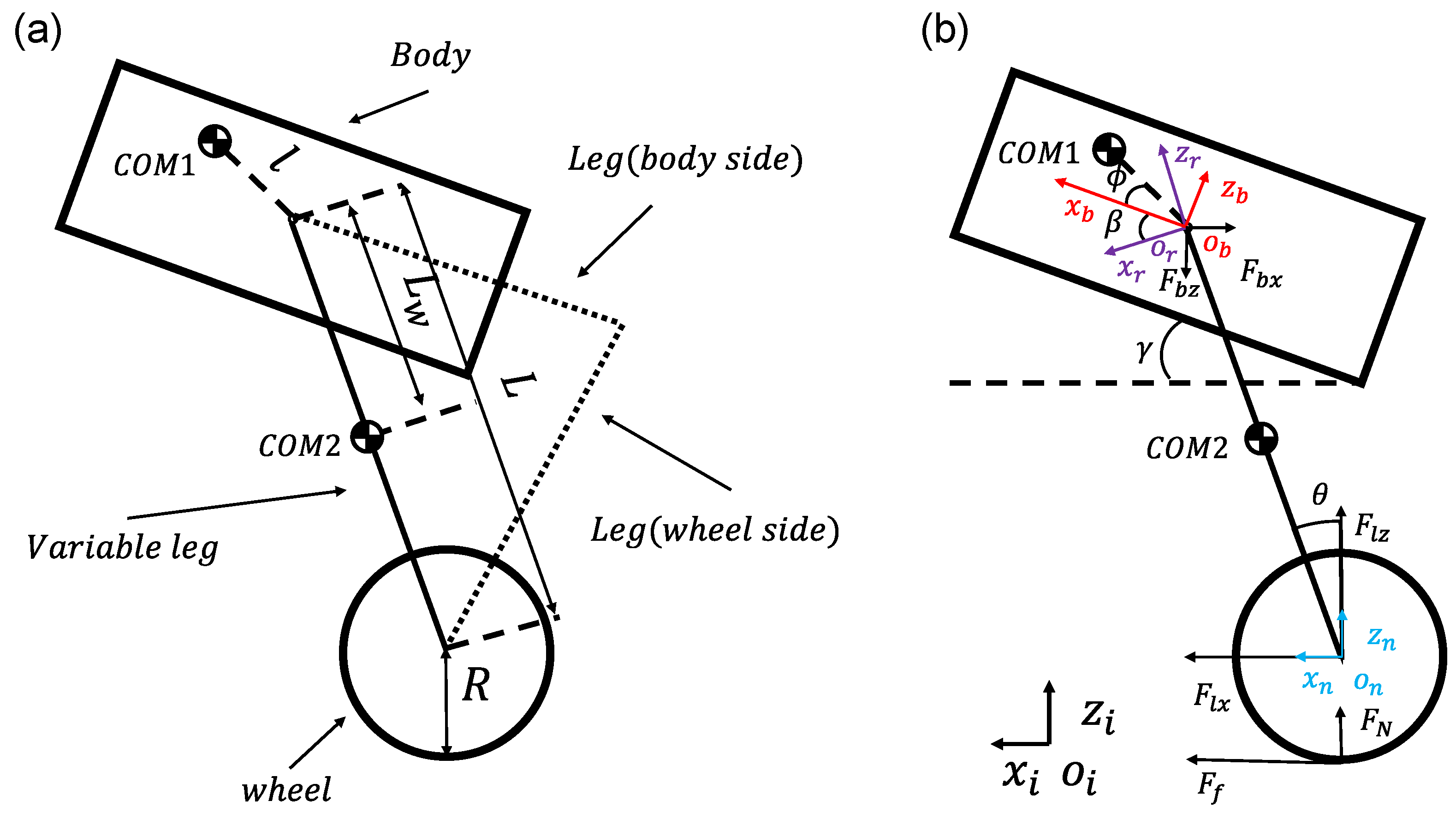
Figure 2a illustrates the physical structure of the WBR and its main components, while Figure 2b shows the corresponding simplified two-dimensional (2D) planar representation in the sagittal $(x$–$z)$ plane used in this work [13]. The virtual leg has an effective length L, which represents the combined geometry of the original leg mechanism. The COM of the robot body is denoted as COM1, whereas COM2 denotes the COM of the virtual leg. The distance from COM2 to the upper end of the virtual leg is denoted by $L_w$, and l represents the distance between the hip joint center and COM1. The wheel radius is denoted by R.

Figure 2. WBR structure. (a) Physical structure of the WBR; (b) two-dimensional (2D) planar representation in the sagittal $(x$–$z)$ plane.

Several coordinate frames are defined to describe the kinematics and dynamics of the robot. The global reference frame $O_i$ is fixed to the ground and serves as a world coordinate frame. The local wheel frame $O_n$ is located at the midpoint between the two wheels and translates along the ground. The body-fixed frame $O_b$ is defined on the robot body, with its origin located at the COM of the body. The leg-fixed frame $O_r$ is attached to the virtual leg. These coordinate frames are illustrated in Figure 2b.

The robot orientation in the sagittal plane is described using several angular variables. The angle $\theta$ denotes the inclination of the virtual leg with respect to the vertical direction. The angle $\beta$ represents the relative rotational angle between the body-fixed frame $O_b$ and the leg-fixed frame $O_r$. The angle $\varphi$ denotes the fixed offset between the COM1 and the local x-axis of the body. The overall pitch angle of the robot body in the sagittal plane is defined as

$$\gamma =\beta +\theta ,$$

(1)

which serves as a key output variable for the subsequent tracking control design [13].

At the wheel–ground contact point, both horizontal and vertical reaction forces act on the system. These forces are denoted by $F_f$ (friction force along the x-direction) and $F_n$ (normal force along the z-direction), respectively. Internal interaction forces between the virtual leg and the body are represented by $(F_{lx},F_{lz})$ for the leg and $(F_{bx},F_{bz})$ for the body. Wheel actuation is provided by the wheel motor torque ${\tau }_w$, while the body motor torque is denoted by ${\tau }_B$.

All physical parameters, including masses, inertias, geometric lengths, and the wheel radius, are summarized in Table 1 [13]. Based on the above coordinate definitions and geometric relationships, the equations of motion are derived using the Newton–Euler formulation and subsequently linearized about the upright equilibrium configuration [13]. The resulting reduced-order planar model forms the basis for the controller design and quantitative performance comparison presented in the following sections.

Table 1. System parameters of the WBR.

Symbol	Description	Value
$I_H$	Inertia about COM of the body	$1.2272\mathrm{kg}{\mathrm{m}}^2$
$I_L$	Inertia about COM of the leg	$0.0130\mathrm{kg}{\mathrm{m}}^2$
$I_w$	Inertia about COM of the wheel	$0.0931\mathrm{kg}{\mathrm{m}}^2$
$M_H$	Mass of the body	$89.7202\mathrm{kg}$
$M_L$	Mass of the leg	$4.4934\mathrm{kg}$
M	Total mass of the robot	$115.9384\mathrm{kg}$
L	Variable leg length	$0.1980\mathrm{m}$
$L_w$	Distance from COM2 to the upper end of the virtual leg	$0.0990\mathrm{m}$
g	Gravitational acceleration	$9.8\mathrm{m}/{\mathrm{s}}^2$
R	Wheel radius	$0.0935\mathrm{m}$

3.2. Assumptions and Model Reduction

To enable tractable controller design and a fair comparison between tracking strategies, the following modeling assumptions are adopted. These assumptions are widely used in WBR and wheeled inverted pendulum studies to focus on the dominant sagittal-plane balance and longitudinal tracking dynamics and to obtain a control-oriented model suitable for analysis and real-time implementation [5,13,15,19]:

• Planar (Sagittal-Plane) Motion Assumption: The robot motion is restricted to the sagittal (x–z) plane. Lateral translation and out-of-plane rotations (yaw and roll), including side-slip effects, are neglected. This assumption isolates the dominant pitch and longitudinal dynamics governing balance and forward motion.
• No-Slip Wheel–Ground Contact: Pure rolling contact is assumed, such that no longitudinal slip occurs. This allows for a direct relationship between wheel torque and longitudinal force. Ground compliance and slip effects are not modeled.
• Rigid-Body Abstraction: The body, leg, and wheel are modeled as rigid bodies with lumped masses and inertias. Structural flexibility, joint backlash, and elastic deformation are neglected.
• Actuator Simplification: Motor and drivetrain dynamics are not explicitly modeled, and actuator torques are treated as direct control inputs to the plant. This simplified torque-input assumption does not explicitly represent actuator bandwidth limitations, internal current-loop dynamics, delays, or torque saturation.

Scope and limitations: Under these assumptions, the model captures the essential sagittal-plane balance and tracking behavior required for evaluating discrete-time tracking controllers in the HILS framework. The results are therefore valid for planar motion around the nominal upright operating condition. Because actuator bandwidth limitations, internal current-loop dynamics, delays, and torque saturation are not explicitly modeled, the reported results should be interpreted as controller comparisons under the simplified torque-actuated plant assumption. In a practical implementation, these actuator-side nonidealities may introduce additional phase lag or input constraints, which can influence transient response and achievable tracking performance. However, because the present formulation is limited to a reduced 3-DOF sagittal-plane model, it does not explicitly represent turning maneuvers, lateral balance recovery, yaw/roll dynamics, or responses to lateral impacts. As a result, neglected lateral and nonlinear dynamics in a full physical WBR system may introduce additional coupling, transient deviations, and degraded tracking or balance performance that are not captured by the present model-based controller design. Three-dimensional effects, uneven terrain, and wheel slip are outside the scope of this study and should be addressed in future work for more realistic full 6-DOF WBR evaluation.

3.3. Equations of Motion and Linearization

The dynamics of the WBR are modeled in the sagittal plane by considering the wheel motor torque, body motor torque, and the longitudinal translational motion along the x-axis [13].

The equations of motion (EoM) of the WBR are given by

$$\begin{array}{cc}\hfill {\tau }_B& =J_1(\ddot{\beta }+\ddot{\theta }),\hfill \\ \hfill {\tau }_w& =J_1(\ddot{\theta }+\ddot{\beta })+J_2\ddot{\theta }+J_3\ddot{x}+J_4\theta ,\hfill \\ \hfill F_w& =J_5\ddot{\theta }+J_6\ddot{x},\hfill \end{array}$$

(2)

where x denotes the horizontal position of the body reference point relative to the global reference frame.

The auxiliary parameters $J_1$–$J_6$ are defined as

$$\begin{array}{cc}\hfill J_1& =I_H,\hfill \end{array}$$

(3)

$$\begin{array}{cc}\hfill J_2& =I_L+L^2{M}_H+L^2{M}_L+L_w^2{M}_L-2L{L}_w{M}_L,\hfill \end{array}$$

(4)

$$\begin{array}{cc}\hfill J_3& =L{M}_H+L{M}_L-L_w{M}_L,\hfill \end{array}$$

(5)

$$\begin{array}{cc}\hfill J_4& =L_w{M}_{L}g-L{M}_{H}g-L{M}_{L}g,\hfill \end{array}$$

(6)

$$\begin{array}{cc}\hfill J_5& =L{M}_H+L{M}_L-L_w{M}_L,\hfill \end{array}$$

(7)

$$\begin{array}{cc}\hfill J_6& =M_H+M_L+{\displaystyle \frac{I_w}{R^2}}.\hfill \end{array}$$

(8)

Here, $J_1$–$J_3$ represent equivalent inertial coupling terms associated with rotational and translational accelerations, $J_4$ corresponds to the gravitational restoring moment acting on the body pitch angle, and $J_5$ and $J_6$ characterize the coupling between wheel rotation and longitudinal translation.

Defining the generalized coordinate vector as

$$\mathbf{q}={\left[\gamma \theta x\right]}^{\top },$$

(9)

where $\gamma =\beta +\theta$ denotes the absolute body pitch angle, the EoM in (2) can be written in compact matrix form as

$$\mathbf{a}\ddot{\mathbf{q}}+\mathbf{b}\mathbf{q}=\mathbf{c}\mathbf{u},$$

(10)

with the input vector $\mathbf{u}={\left[{\tau }_B{\tau }_w\right]}^{\top }$. The matrices are defined as

$$\mathbf{a}={\displaystyle \frac{\partial f\left(\mathrm{EoM}\right)}{\partial \ddot{\mathbf{q}}}},\mathbf{b}={\displaystyle \frac{\partial f\left(\mathrm{EoM}\right)}{\partial \mathbf{q}}},\mathbf{c}=\left[\begin{array}{cc}-1& 0\\ 0& -1\\ 0& {\displaystyle \frac{1}{R}}\end{array}\right].$$

(11)

By introducing the state vector

$$\mathbf{x}\left(t\right)={\left[\gamma \theta x\dot{\gamma }\dot{\theta }\dot{x}\right]}^{\top },$$

(12)

the system can be expressed in continuous-time state-space form as

$$\dot{\mathbf{x}}\left(t\right)=\mathbf{A}\mathbf{x}\left(t\right)+\mathbf{B}\mathbf{u}\left(t\right),$$

(13)

where

$$\mathbf{A}=\left[\begin{array}{cc}{\mathbf{0}}_{3\times 3}& {\mathbf{I}}_{3\times 3}\\ -{\mathbf{a}}^{-1}\mathbf{b}& {\mathbf{0}}_{3\times 3}\end{array}\right],\mathbf{B}=\left[\begin{array}{c}{\mathbf{0}}_{3\times 2}\\ {\mathbf{a}}^{-1}\mathbf{c}\end{array}\right].$$

(14)

The linearized model in (13) is obtained around the upright equilibrium point defined by

$$\gamma =0,\theta =0,x=0,\dot{\gamma }=\dot{\theta }=\dot{x}=0,$$

(15)

with zero input torques. This equilibrium corresponds to a balanced upright posture without translational motion.

4. Controller Design

The WBR considered in this study exhibits inherently unstable dynamics arising from its underactuated structure and inverted-pendulum configuration. In the absence of appropriate feedback control, the robot is unable to maintain balance or achieve accurate tracking of commanded motions. Hence, a stabilizing servo controller is required to ensure (i) internal stabilization and (ii) accurate reference tracking of task-level outputs over time, even in the presence of modeling uncertainty, external disturbances, and measurement noise.

This paper implements and compares two linear servo-control strategies based on a linearized state-space model: FSF control and LQ-Servo control [7]. FSF is simple to implement and can yield fast transient responses under nominal conditions, but it does not include integral action and therefore may exhibit steady-state tracking errors in the presence of constant disturbances or modeling bias. LQ-Servo extends the classical LQR by augmenting integral states of the output tracking error, enabling disturbance rejection and steady-state error elimination while preserving an optimal trade-off between performance and control effort through a quadratic cost function. In the following subsections, both controllers are formulated in a unified framework to facilitate a fair comparison [5].

4.1. FSF Tracking Controller

Consider the linearized plant

$$\dot{\mathbf{x}}\left(t\right)=\mathbf{A}\mathbf{x}\left(t\right)+\mathbf{B}\mathbf{u}\left(t\right),$$

(16)

where $\mathbf{x}\left(t\right)\in {\mathbb{R}}^n$ and $\mathbf{u}\left(t\right)\in {\mathbb{R}}^m$ denote the state and control input, respectively. For trajectory tracking, a differentiable reference state trajectory ${\mathbf{x}}_r\left(t\right)$ is assumed, representing the desired output reference.

The state tracking error is defined as

$${\mathbf{e}}_x\left(t\right)=\mathbf{x}\left(t\right)-{\mathbf{x}}_r\left(t\right).$$

(17)

Differentiating (17) and using (16) yields

$${\dot{\mathbf{e}}}_x\left(t\right)=\mathbf{A}\left({\mathbf{e}}_x\left(t\right)+{\mathbf{x}}_r\left(t\right)\right)+\mathbf{B}\mathbf{u}\left(t\right)-{\dot{\mathbf{x}}}_r\left(t\right).$$

(18)

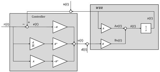
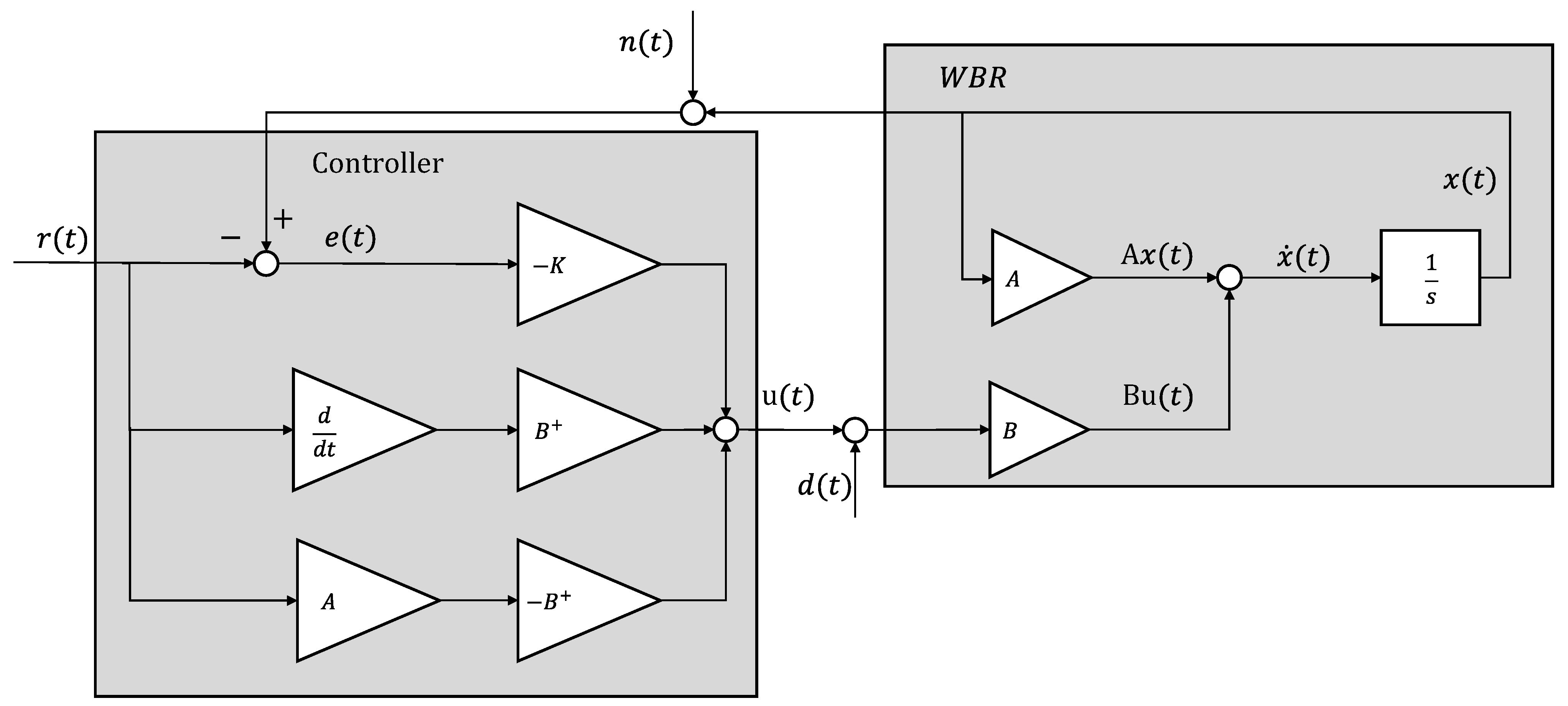
If the control input is chosen as

$$\mathbf{u}\left(t\right)={\mathbf{B}}^{+}\left({\dot{\mathbf{x}}}_r\left(t\right)-\mathbf{A}{\mathbf{x}}_r\left(t\right)\right)-\mathbf{K}{\mathbf{e}}_x\left(t\right),$$

(19)

where ${\mathbf{B}}^{+}$ denotes the Moore–Penrose pseudoinverse of $\mathbf{B}$; then, substituting (19) into (18) yields

$$\begin{array}{cc}\hfill {\dot{\mathbf{e}}}_x\left(t\right)& =\mathbf{A}\left({\mathbf{e}}_x\left(t\right)+{\mathbf{x}}_r\left(t\right)\right)+\mathbf{B}\left[{\mathbf{B}}^{+}\left({\dot{\mathbf{x}}}_r\left(t\right)-\mathbf{A}{\mathbf{x}}_r\left(t\right)\right)-\mathbf{K}{\mathbf{e}}_x\left(t\right)\right]-{\dot{\mathbf{x}}}_r\left(t\right)\hfill \\ \hfill & =(\mathbf{A}-\mathbf{B}\mathbf{K}){\mathbf{e}}_x\left(t\right)+\left(\mathbf{B}{\mathbf{B}}^{+}-\mathbf{I}\right)\left({\dot{\mathbf{x}}}_r\left(t\right)-\mathbf{A}{\mathbf{x}}_r\left(t\right)\right).\hfill \end{array}$$

(20)

If the reference satisfies the consistency condition ${\dot{\mathbf{x}}}_r\left(t\right)-\mathbf{A}{\mathbf{x}}_r\left(t\right)\in \mathcal{R}\left(\mathbf{B}\right)$, then $\mathbf{B}{\mathbf{B}}^{+}\left({\dot{\mathbf{x}}}_r\left(t\right)-\mathbf{A}{\mathbf{x}}_r\left(t\right)\right)={\dot{\mathbf{x}}}_r\left(t\right)-\mathbf{A}{\mathbf{x}}_r\left(t\right)$ and the residual term in (20) vanishes. The second term represents a reference-consistency residual that appears when the reference signal is not exactly realizable through the input channel. In this work, the residual is monitored.

$${\mathbf{r}}_{\mathrm{res}}\left(t\right)\triangleq \left(\mathbf{I}-\mathbf{B}{\mathbf{B}}^{+}\right)\left({\dot{\mathbf{x}}}_r\left(t\right)-\mathbf{A}{\mathbf{x}}_r\left(t\right)\right),$$

(21)

In Section 5, it will be confirmed that this remains negligible (within numerical tolerance) for the adopted reference trajectory under the real-time HILS setup. Accordingly, when ${\mathbf{r}}_{\mathrm{res}}\left(t\right)\approx \mathbf{0}$, the FSF error dynamics reduce to

$${\dot{\mathbf{e}}}_x\left(t\right)=(\mathbf{A}-\mathbf{B}\mathbf{K}){\mathbf{e}}_x\left(t\right).$$

(22)

The feedback gain $\mathbf{K}$ is designed via the standard continuous-time LQR for $(\mathbf{A},\mathbf{B})$. Since the feedforward term depends only on the reference, $\mathbf{K}$ is obtained by minimizing

$$J_{\mathrm{FSF}}={\int }_0^{\infty }\left({\mathbf{e}}_x^{\top }\left(t\right)\mathbf{Q}{\mathbf{e}}_x\left(t\right)+{\mathbf{u}}_{\mathrm{fb}}^{\top }\left(t\right)\mathbf{R}{\mathbf{u}}_{\mathrm{fb}}\left(t\right)\right)dt,{\mathbf{u}}_{\mathrm{fb}}\left(t\right)=-\mathbf{K}{\mathbf{e}}_x\left(t\right),$$

(23)

where $\mathbf{Q}⪰0$ and $\mathbf{R}\succ 0$ are the state and input weighting matrices. The optimal gain is computed from the continuous-time algebraic Riccati equation

$${\mathbf{A}}^{\top }\mathbf{P}+\mathbf{P}\mathbf{A}-\mathbf{P}\mathbf{B}{\mathbf{R}}^{-1}{\mathbf{B}}^{\top }\mathbf{P}+\mathbf{Q}=0,$$

(24)

as

$$\mathbf{K}={\mathbf{R}}^{-1}{\mathbf{B}}^{\top }\mathbf{P}.$$

(25)

Figure 3 illustrates the FSF tracking structure: the control input $\mathbf{u}\left(t\right)$ is generated from the reference-dependent feedforward term and the feedback term based on the state tracking error, ensuring closed-loop stability and reference tracking under nominal conditions.

Figure 3. FSF Structure.

4.2. LQ-Servo Control with Integral Augmentation

The pitch angle $\gamma$ must track a desired reference to maintain a stable upright posture during locomotion or task execution. Depending on the task, this reference may be nonzero to achieve dynamic balance. The longitudinal position x must track a commanded trajectory to enable purposeful motion. Therefore, both $\gamma$ and x are treated as servo-tracking outputs.

In contrast, the internal joint angle $\theta$ is regulated around its equilibrium point rather than explicitly tracked. Regulating $\theta$ promotes internal stability and posture consistency, but it does not directly represent a task-level objective. Hence, $\theta$ is handled through a regulator-type objective rather than servo tracking.

Given a reference trajectory

$$\mathbf{r}\left(t\right)=\left[\begin{array}{c}{\gamma }_r\left(t\right)\\ x_r\left(t\right)\end{array}\right]\in {\mathbb{R}}^p,(p=2),$$

(26)

an LQ-Servo controller is designed to eliminate steady-state tracking error and improve disturbance rejection by augmenting the plant with integral states of the output tracking error. Let the measured/controlled output be

$$\mathbf{y}\left(t\right)={\mathbf{C}}_y\mathbf{x}\left(t\right),$$

(27)

where $\mathbf{y}\left(t\right)={\left[\gamma \left(t\right)x\left(t\right)\right]}^{\top }$ is the servo-tracking output vector and ${\mathbf{C}}_y\in {\mathbb{R}}^{p\times n}$ selects the pitch angle and longitudinal position from the state. For the state ordering used in this work, ${\mathbf{C}}_y$ is chosen as

$${\mathbf{C}}_y=\left[\begin{array}{cccccc}1& 0& 0& 0& 0& 0\\ 0& 0& 1& 0& 0& 0\end{array}\right].$$

(28)

Given the output reference $\mathbf{r}\left(t\right)\in {\mathbb{R}}^p$, the output tracking error is

$${\mathbf{e}}_y\left(t\right)=\mathbf{r}\left(t\right)-\mathbf{y}\left(t\right)=\mathbf{r}\left(t\right)-{\mathbf{C}}_y\mathbf{x}\left(t\right).$$

(29)

The integral state is defined as

$${\dot{\mathbf{x}}}_I\left(t\right)={\mathbf{e}}_y\left(t\right),$$

(30)

and the augmented state is constructed as

$$\overline{\mathbf{x}}\left(t\right)=\left[\begin{array}{c}\mathbf{x}\left(t\right)\\ {\mathbf{x}}_I\left(t\right)\end{array}\right].$$

(31)

Combining (16), (27) and (30), the augmented dynamics are written as

$$\dot{\overline{\mathbf{x}}}\left(t\right)=\overline{\mathbf{A}}\overline{\mathbf{x}}\left(t\right)+\overline{\mathbf{B}}\mathbf{u}\left(t\right)+\overline{\mathbf{E}}\mathbf{r}\left(t\right),$$

(32)

where

$$\overline{\mathbf{A}}=\left[\begin{array}{cc}\mathbf{A}& \mathbf{0}\\ -{\mathbf{C}}_y& \mathbf{0}\end{array}\right],\overline{\mathbf{B}}=\left[\begin{array}{c}\mathbf{B}\\ \mathbf{0}\end{array}\right],\overline{\mathbf{E}}=\left[\begin{array}{c}\mathbf{0}\\ \mathbf{I}\end{array}\right],$$

(33)

and $\mathbf{I}\in {\mathbb{R}}^{p\times p}$ is the identity matrix. Note that the LQ-Servo gain is designed for the pair $(\overline{\mathbf{A}},\overline{\mathbf{B}})$, treating $\mathbf{r}\left(t\right)$ as an exogenous input through $\overline{\mathbf{E}}$.

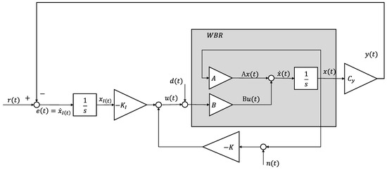
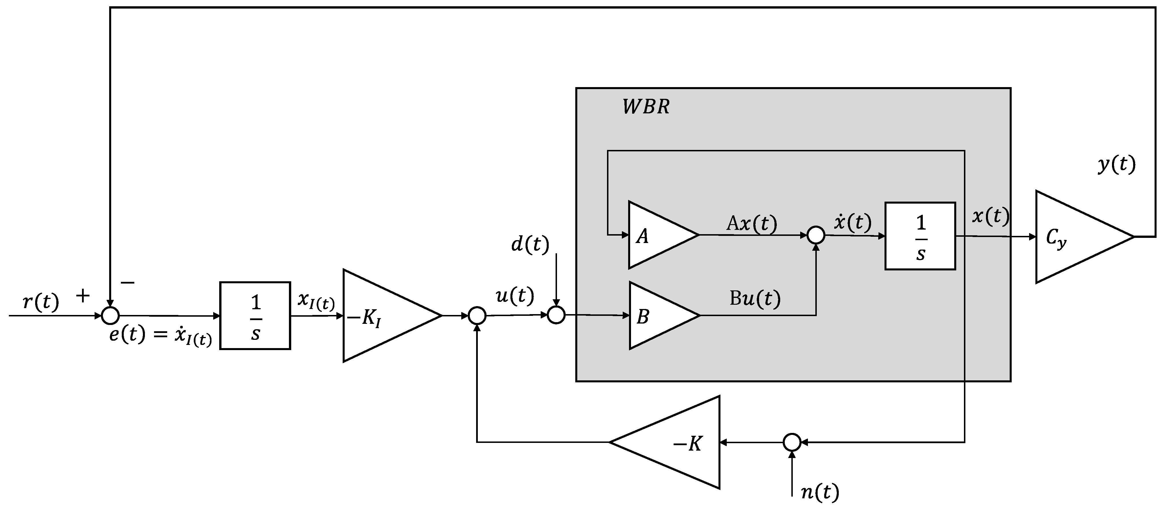
The LQ-Servo control law is defined as

$$\mathbf{u}\left(t\right)=-\left[\begin{array}{cc}\mathbf{K}& {\mathbf{K}}_I\end{array}\right]\left[\begin{array}{c}\mathbf{x}\left(t\right)\\ {\mathbf{x}}_I\left(t\right)\end{array}\right]=-\overline{\mathbf{K}}\overline{\mathbf{x}}\left(t\right),$$

(34)

where $\mathbf{K}\in {\mathbb{R}}^{m\times n}$ and ${\mathbf{K}}_I\in {\mathbb{R}}^{m\times p}$ denote the proportional (state) and integral gains, respectively, and $\overline{\mathbf{K}}=\left[\mathbf{K}{\mathbf{K}}_I\right]$. The gain $\overline{\mathbf{K}}$ is obtained by applying the continuous-time LQR design to the augmented system (32) with respect to the control input $\mathbf{u}\left(t\right)$. Specifically, the quadratic cost

$$J={\int }_0^{\infty }\left({\overline{\mathbf{x}}}^{\top }\left(t\right)\overline{\mathbf{Q}}\overline{\mathbf{x}}\left(t\right)+{\mathbf{u}}^{\top }\left(t\right)\mathbf{R}\mathbf{u}\left(t\right)\right)dt$$

(35)

is minimized, where $\overline{\mathbf{Q}}⪰0$ and $\mathbf{R}\succ 0$ are weighting matrices. The optimal gain is computed via the algebraic Riccati equation associated with $(\overline{\mathbf{A}},\overline{\mathbf{B}})$, and the resulting feedback gain is

$$\overline{\mathbf{K}}={\mathbf{R}}^{-1}{\overline{\mathbf{B}}}^{\top }\overline{\mathbf{P}},$$

(36)

where $\overline{\mathbf{P}}$ is the positive semidefinite stabilizing solution of the corresponding Riccati equation.

Substituting the control law (34) into (32) yields the overall closed-loop augmented dynamics:

$$\dot{\overline{\mathbf{x}}}\left(t\right)=\left(\overline{\mathbf{A}}-\overline{\mathbf{B}}\overline{\mathbf{K}}\right)\overline{\mathbf{x}}\left(t\right)+\overline{\mathbf{E}}\mathbf{r}\left(t\right).$$

(37)

Equivalently, in block-matrix form,

$$\left[\begin{array}{c}\dot{\mathbf{x}}\left(t\right)\\ {\dot{\mathbf{x}}}_I\left(t\right)\end{array}\right]=\left[\begin{array}{cc}\mathbf{A}-\mathbf{B}\mathbf{K}& -\mathbf{B}{\mathbf{K}}_I\\ -{\mathbf{C}}_y& \mathbf{0}\end{array}\right]\left[\begin{array}{c}\mathbf{x}\left(t\right)\\ {\mathbf{x}}_I\left(t\right)\end{array}\right]+\left[\begin{array}{c}\mathbf{0}\\ \mathbf{I}\end{array}\right]\mathbf{r}\left(t\right).$$

(38)

Figure 4 illustrates the LQ-Servo structure. By combining proportional state feedback with integral action on the output tracking error, the proposed controller achieves reference tracking and improves steady-state disturbance rejection compared with the FSF controller.

Figure 4. LQ-Servo structure.

4.3. Stability and Practical Implementation Notes

4.3.1. LQR Weighting Selection and Gain Computation

To evaluate stability margins and robustness metrics, the feedback gains must be fixed a priori. Accordingly, the LQR weighting matrices are first specified, and the stabilizing gains are then computed from the corresponding continuous-time algebraic Riccati equations.

For both controllers, the same input penalty is used for a fair comparison. Because maintaining body balance is critical for the stability of the wheeled bipedal robot, the input penalty is selected to be relatively small so that sufficient control authority is available to rapidly correct posture deviations while still avoiding unnecessarily large control inputs:

$$\mathbf{R}=0.1{\mathbf{I}}_2.$$

(39)

For FSF, the state penalty is chosen as

$$\mathbf{Q}=\mathrm{diag}\left([5,5,10,3,3,3]\right),$$

(40)

For LQ-Servo, the plant is augmented with integral states of the output tracking error; thus $\mathbf{Q}$ is expanded to match the augmented state dimension:

$$\overline{\mathbf{Q}}=\mathrm{blkdiag}\left(\mathbf{Q},10{\mathbf{I}}_p\right),\overline{\mathbf{R}}=\mathbf{R},(p=2).$$

(41)

The added weight 10 matches the largest entry in $\mathbf{Q}$ and emphasizes the integral (tracking-error) states, which are the key quantities for steady-state accuracy in LQ-Servo.

4.3.2. Closed-Loop Stability Condition

Using the gains computed from the weighting matrices in (40) and (41), the internal stability of the FSF design requires the closed-loop matrix $(\mathbf{A}-\mathbf{B}\mathbf{K})$ to be Hurwitz. Likewise, the internal stability of the LQ-Servo design requires the augmented closed-loop matrix

$${\overline{\mathbf{A}}}_{\mathrm{cl}}=\overline{\mathbf{A}}-\overline{\mathbf{B}}\overline{\mathbf{K}}=\left[\begin{array}{cc}\mathbf{A}-\mathbf{B}\mathbf{K}& -\mathbf{B}{\mathbf{K}}_I\\ -{\mathbf{C}}_y& \mathbf{0}\end{array}\right]$$

(42)

to be Hurwitz.

4.3.3. Robustness Metrics ($M_s$, $M_t$, and Multiloop Disk Margin (DM))

After fixing $\mathbf{K}$ (FSF) and $\overline{\mathbf{K}}$ (LQ-Servo) via the LQR/LQ-Servo designs described above, nominal MIMO loop robustness is evaluated using the input-side return ratio, defined consistently with each controller realization: for FSF,

$$L_{\mathrm{FSF}}\left(s\right)=\mathbf{K}{(s\mathbf{I}-\mathbf{A})}^{-1}\mathbf{B}\in {\mathbb{R}}^{m\times m},(m=2),$$

(43)

whereas for LQ-Servo (which includes the integral state), the augmented loop is used,

$$L_{\mathrm{LQ}}\left(s\right)=\overline{\mathbf{K}}{(s\mathbf{I}-\overline{\mathbf{A}})}^{-1}\overline{\mathbf{B}}\in {\mathbb{R}}^{m\times m}.$$

(44)

with $(\overline{\mathbf{A}},\overline{\mathbf{B}})$ denoting the augmented plant. For each case, the sensitivity and complementary sensitivity are computed from the corresponding $L\left(s\right)$ as

$$S\left(s\right)={(\mathbf{I}+L\left(s\right))}^{-1},T\left(s\right)=L\left(s\right){(\mathbf{I}+L\left(s\right))}^{-1},$$

(45)

and the corresponding peak values $M_s={\parallel S\parallel }_{\infty }$ and $M_t={\parallel T\parallel }_{\infty }$ are reported together with multiloop disk margins [20,22,28,30].

As summarized in Table 2, both controllers yield $M_s\approx 1.00$, indicating negligible sensitivity peaking for the nominal loop. The FSF controller achieves a smaller complementary-sensitivity peak ($M_t=1.2268$) than LQ-Servo ($M_t=1.4413$). Regarding multiloop disk margins, FSF provides a larger robustness margin (DM $=1.2470$) with wider gain and phase margins ($[0.2319,4.3124]$, $\pm 63.{89}^{\circ }$) than LQ-Servo (DM $=1.0007$, $[0.3330,3.0029]$, $\pm 53.{16}^{\circ }$). The worst-case frequencies ${\omega }^{★}$ are also reported in Table 2, indicating that the limiting robustness occurs near $0.92\mathrm{rad}/\mathrm{s}$ for FSF and $1.19\mathrm{rad}/\mathrm{s}$ for LQ-Servo.

Table 2. Robustness metrics for FSF and LQ-Servo controllers (input-side MIMO loop). Here, ${\omega }^{★}$ denotes the worst-case frequency at which the limiting robustness occurs. Loop-at-a-time DM #1 and #2 denote the disk margins associated with the first and second input channels, respectively.

Controller	${\mathit{M}}_{\mathit{s}}={\parallel \mathit{S}\parallel }_{\mathit{\infty }}$	${\mathit{M}}_{\mathit{t}}={\parallel \mathit{T}\parallel }_{\mathit{\infty }}$	Multiloop DM	${\mathit{\omega }}^{\mathbf{★}}$ (rad/s)
FSF	1.0000	1.2268	1.2470	0.9171
LQ-Servo	1.0000	1.4413	1.0007	1.1920
Controller	Loop-at-a-Time DM #1	Loop-at-a-Time DM #2	Multiloop Gain Margin $[{\mathit{g}}_{\mathit{L}},{\mathit{g}}_{\mathit{U}}]$	Multiloop Phase Margin (deg)
FSF	1.5375	1.2511	[0.2319, 4.3124]	$\pm 63.89$
LQ-Servo	1.2957	1.0033	[0.3330, 3.0029]	$\pm 53.16$

4.3.4. Discrete-Time Realization of the ZOH-Equivalent Plant Model

Since the HILS target machine simulates the plant in discrete time, the plant is discretized and expressed as the Zero-Order Hold (ZOH)-equivalent model of the linearized continuous-time dynamics $\dot{\mathbf{x}}\left(t\right)=\mathbf{A}\mathbf{x}\left(t\right)+\mathbf{B}\mathbf{u}\left(t\right)$:

$$\mathbf{x}[k+1]={\mathbf{A}}_d\mathbf{x}\left[k\right]+{\mathbf{B}}_d\mathbf{u}\left[k\right],{\mathbf{A}}_d=e^{\mathbf{A}{T}_s},{\mathbf{B}}_d={\int }_0^{T_s}{e}^{\mathbf{A}\tau }\mathbf{B}d\tau .$$

(46)

4.3.5. Bandwidth-Based Rationale for Selecting the Sampling Period

The HILS sampling period was selected to be sufficiently smaller than the minimum sampling-time bound identified from the modal-bandwidth and FRF-based bandwidth criteria, while remaining compatible with the real-time computational capability of the HILS target machine [31].

The modal bandwidth reflects the fastest intrinsic mode of the linearized dynamics, whereas the FRF-based bandwidth was additionally considered because some open-loop channels, particularly those associated with absolute position states, may exhibit integrator-like behavior for which a standard $-3$ dB bandwidth is not always well defined [32,33]. The detailed definitions of these bandwidth measures and the channel-wise FRF results are provided in Appendix B.

For the present system, the modal bandwidth was identified as $4.15\mathrm{Hz}$, while the maximum valid FRF-based bandwidth was identified as $6.45\mathrm{Hz}$. A conservative representative bandwidth was therefore selected from the larger of these two values. Based on this representative bandwidth, the Nyquist lower-bound sampling condition and the practical $10\times$ bandwidth rule yield a recommended sampling period that is substantially larger than the adopted HILS sampling period. Accordingly, the implemented $T_s=1\mathrm{ms}$ can be regarded as sufficiently small for representing the dominant model dynamics in the sampled-data HILS implementation.

To illustrate the discrete-time stability tendency at representative sampling times, Table 3 lists the spectral radius of the nominal sampled-data closed-loop systems for FSF and LQ-Servo. For both controllers, the spectral radius remained below unity at the HILS sampling period and at the sampling period corresponding to the practical $10\times$ bandwidth rule. By contrast, when the sampling period was increased to the Nyquist lower-bound level, the spectral radius exceeded unity for both controllers, indicating sampled-data instability.

Table 3. Spectral radius of the sampled-data closed-loop systems at representative sampling times (nominal case).

Controller	${\mathit{T}}_{\mathit{s}}$ (ms)	Spectral Radius $\mathit{\rho }$
FSF	1.0000	0.99938
	15.5017	0.99034
	77.5085	2.74990
LQ-Servo	1.0000	0.99943
	15.5017	0.99124
	77.5085	2.82360

The results in Table 3 show that the proposed sampled-data implementation remains stable within this practically relevant range, whereas a much slower sampling rate near the Nyquist lower bound renders both controllers unstable.

4.3.6. Discrete-Time Realization of the FSF Tracking Controller

The FSF controller is implemented in discrete time on the embedded processor using sampled signals $\mathbf{x}\left[k\right]$ and ${\mathbf{x}}_r\left[k\right]$. The state tracking error is defined as

$${\mathbf{e}}_x\left[k\right]=\mathbf{x}\left[k\right]-{\mathbf{x}}_r\left[k\right].$$

(47)

To avoid explicit reference derivatives in implementation, the reference-dependent feedforward term is constructed from the discrete-time consistency relation ${\mathbf{x}}_r[k+1]\approx {\mathbf{A}}_d{\mathbf{x}}_r\left[k\right]+{\mathbf{B}}_d{\mathbf{u}}_{\mathrm{ff}}\left[k\right]$, yielding

$${\mathbf{u}}_{\mathrm{ff}}\left[k\right]={\mathbf{B}}_d^{+}\left({\mathbf{x}}_r[k+1]-{\mathbf{A}}_d{\mathbf{x}}_r\left[k\right]\right),$$

(48)

where ${\mathbf{B}}_d^{+}$ is the Moore–Penrose pseudoinverse of ${\mathbf{B}}_d$. Accordingly, the sampled FSF control computation becomes

$${\mathbf{u}}_c\left[k\right]={\mathbf{u}}_{\mathrm{ff}}\left[k\right]-\mathbf{K}{\mathbf{e}}_x\left[k\right].$$

(49)

In practice, the motor torques are bounded, $\mathbf{u}\left(t\right)\in \mathcal{U}$, and the applied command is clipped to satisfy actuator limits (ZOH actuation), i.e.,

$$\mathbf{u}\left(t\right)=\mathbf{u}\left[k\right],t\in [k{T}_s,(k+1)T_s),\mathbf{u}\left[k\right]={\mathrm{sat}}_{\mathcal{U}}\left({\mathbf{u}}_c\left[k\right]\right).$$

(50)

4.3.7. Discrete-Time Realization of the LQ-Servo Controller

The LQ-Servo controller is implemented in discrete time on the embedded processor in the same manner, using the sampled signals $\mathbf{x}\left[k\right]$ and $\mathbf{r}\left[k\right]$. The continuous-time integral state ${\dot{\mathbf{x}}}_I\left(t\right)=\mathbf{r}\left(t\right)-{\mathbf{C}}_y\mathbf{x}\left(t\right)$ is discretized using a forward-Euler update:

$${\mathbf{x}}_I[k+1]={\mathbf{x}}_I\left[k\right]+T_s\left(\mathbf{r}\left[k\right]-{\mathbf{C}}_y\mathbf{x}\left[k\right]\right).$$

(51)

With the sampled integral state, the discrete-time control computation becomes

$${\mathbf{u}}_c\left[k\right]=-\mathbf{K}\mathbf{x}\left[k\right]-{\mathbf{K}}_I{\mathbf{x}}_I\left[k\right].$$

(52)

The applied command is held constant over each sampling interval and clipped to satisfy actuator limits:

$$\mathbf{u}\left(t\right)=\mathbf{u}\left[k\right],t\in [k{T}_s,(k+1)T_s),\mathbf{u}\left[k\right]={\mathrm{sat}}_{\mathcal{U}}\left({\mathbf{u}}_c\left[k\right]\right).$$

(53)

When actuator saturation is active, the integral state may continue to accumulate the tracking error even though the commanded input cannot be realized, which can lead to integral windup and degrade transient recovery [29,34]. In our embedded implementation, this is mitigated with a lightweight anti-windup safeguard applied only to the integral channel, without altering the nominal LQ-Servo gain design.

$$x_{I,i}[k+1]={\mathrm{sat}}_{[-X_{I,i}^{max},X_{I,i}^{max}]}\left(x_{I,i}\left[k\right]+T_s{e}_{y,i}\left[k\right]\right),i=1,\dots ,p.$$

(54)

This integrator-clamping structure limits the excessive accumulation of the integral channel and helps reduce prolonged recovery, excessive overshoot, and undesirable transient behavior, while leaving the nominal closed-loop design unchanged in the unsaturated regime.

5. Real-Time HILS Evaluation

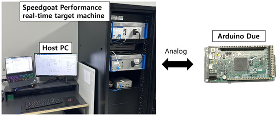
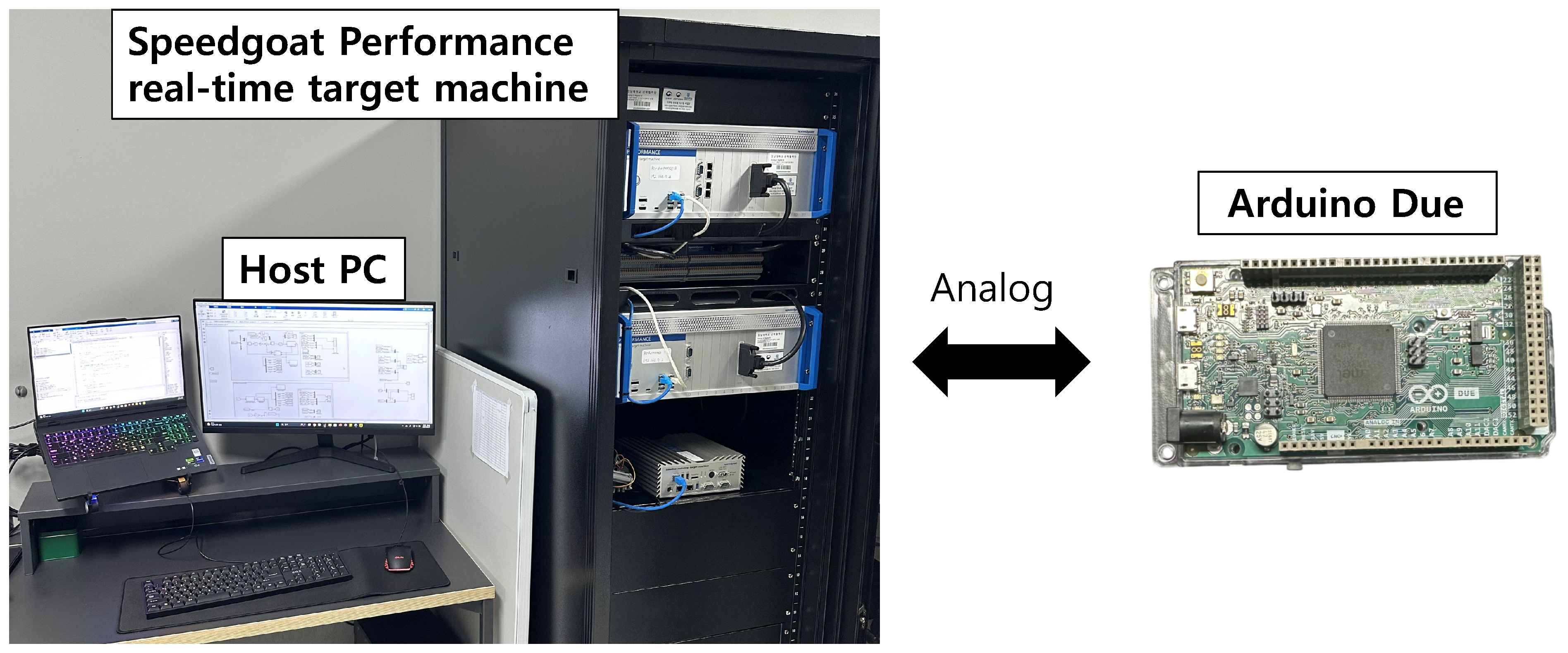
This section reports the real-time HILS results for the FSF and LQ-Servo controllers. HILS has become a standard verification paradigm in control engineering, serving as an essential bridge between numerical software simulation and full-scale physical testing [23,24,25]. The controller is executed on an Arduino Due with a fixed sampling period of $T_s=1\mathrm{ms}$, while the linearized WBR plant is simulated on a Speedgoat real-time target as the same fixed sampling period. Six state channels are transmitted to the controller and two torque commands are returned to the plant via analog I/O. The signal exchange between the Speedgoat real-time target and the controller hardware is implemented using an IO133 analog I/O module. The plant-side state variables are converted to analog voltage signals and transmitted to the controller, while the controller-generated torque commands are returned to the plant through analog output channels. Figure 5 shows the overall HILS setup.

Figure 5. Real-time HILS setup and signal flow between the Arduino Due controller and the Speedgoat real-time target.

For completeness, the reference-consistency residual ${\mathbf{r}}_{\mathrm{res}}\left(t\right)$ defined in (21) was numerically checked during the real-time HILS evaluation and was identically zero throughout the experiment.

5.1. Test Cases and Metrics

Both controllers are evaluated under the following five conditions:

• Nominal (LQ, FSF): Nominal parameters without injected disturbance.
• Uncertainty Only (LQ_C, FSF_C): Nominal disturbance-free operation with parametric perturbations ($M_H=1.5M_{H0}$, $L=1.01L_0$).
• Disturbance Only (LQ_D, FSF_D): A constant bias torque $d_W$ is added to the wheel-torque channel ${\tau }_w$.
• Disturbance + Uncertainty (LQ_DC, FSF_DC): The wheel disturbance is applied together with parametric perturbations.
• Time-Varying Sine Disturbance (LQ_S0.2Hz, FSF_S0.2Hz, LQ_S1Hz, FSF_S1Hz): An additional sinusoidal disturbance with amplitude 1 is injected into the wheel-torque disturbance channel. Two excitation frequencies are considered: $0.2\mathrm{Hz}$ and $1\mathrm{Hz}$.

Tracking performance is quantified using the Integral of Squared Error (ISE) for $\gamma$, $\theta$, and x. For the longitudinal position x, step-response metrics are additionally computed, including percent overshoot (P.O.), rise time ($t_r$), settling time ($t_s$), and steady-state error ($e_{ss}$). The settling band is defined as $\pm 0.05\mathrm{m}$ around the reference. To complement these tracking-oriented measures, actuator-related input metrics are also evaluated from the body- and wheel-torque commands. Specifically, the integral of squared torque is used to quantify cumulative control effort, the RMS torque is used to represent sustained actuator demand, and the peak absolute torque is used to indicate the maximum instantaneous actuator requirement.

5.2. Real-Time Response Results

5.2.1. Nominal Tracking

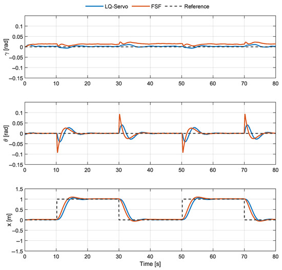
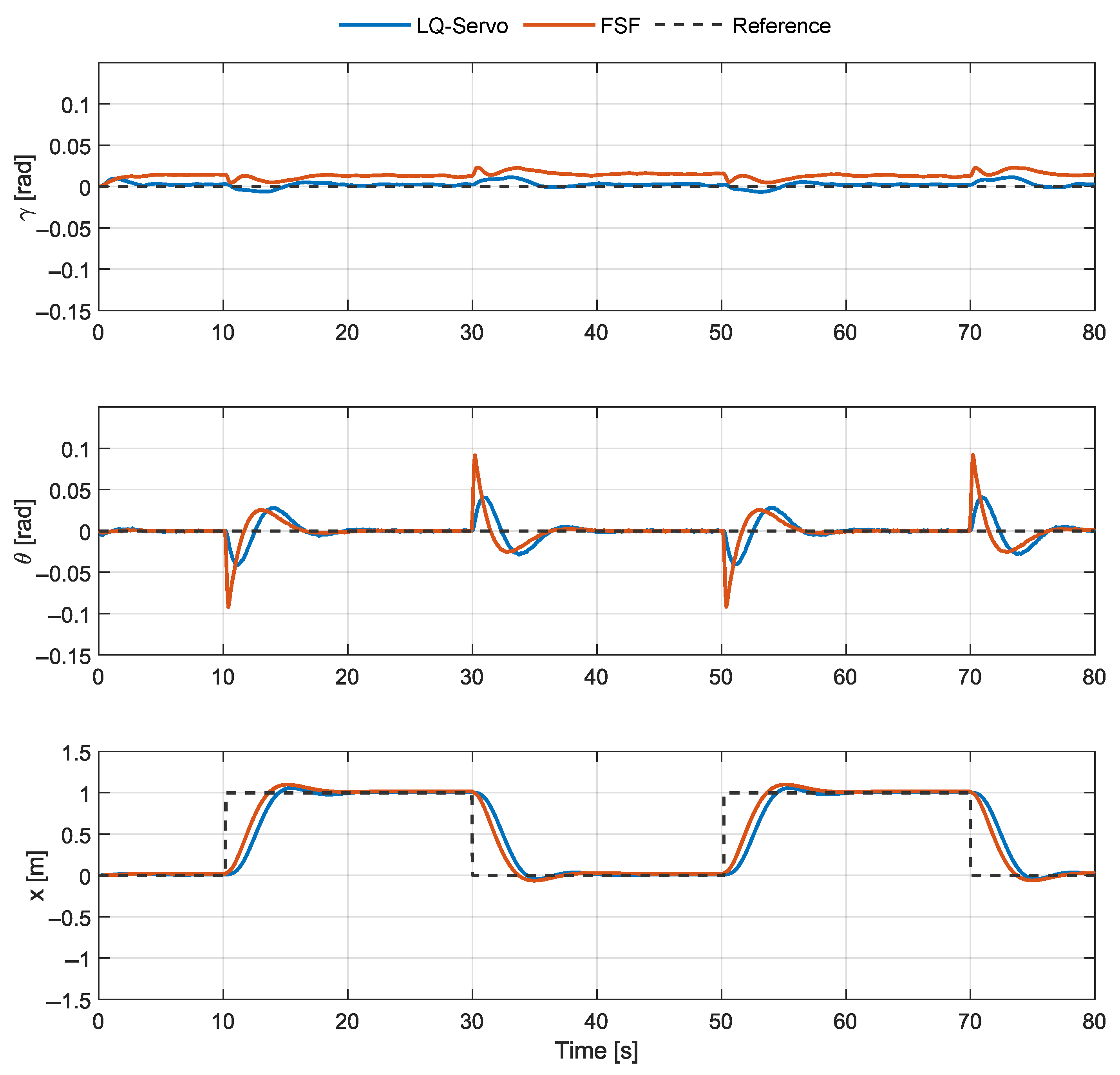
Figure 6 shows the nominal real-time response to an alternating position command ($x:0\leftrightarrow 1\mathrm{m}$). Both controllers maintain $\gamma$ near the equilibrium and track the commanded x. Transient variations in $\theta$ are observed at each step transition.

Figure 6. Nominal real-time HILS response: LQ-Servo vs. FSF.

5.2.2. External Disturbance Response

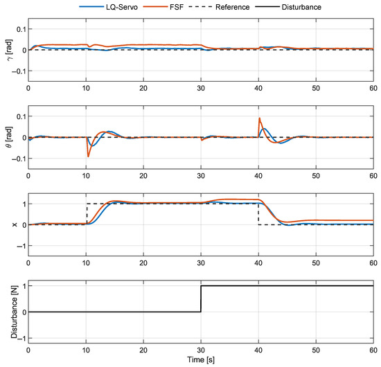
Figure 7 presents the response under a constant bias torque applied to ${\tau }_w$, which was selected to represent a persistent external disturbance such as an uphill-road condition. A steady offset in x is observed for FSF_D, measured at approximately $0.205\mathrm{m}$, while LQ_D returns x to the commanded reference after a transient deviation (approximately $0.08\mathrm{m}$ peak). Both cases keep $\gamma$ close to zero.

Figure 7. Real-time HILS response under wheel-torque disturbance.

5.2.3. Control Inputs

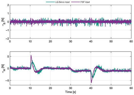
Figure 8 shows the commanded torques during HILS. The body torque ${\tau }_B$ remains within approximately $\pm 0.5\mathrm{N}·\mathrm{m}$, while the wheel torque ${\tau }_w$ reaches peaks of approximately $\pm 5\mathrm{N}·\mathrm{m}$ during transitions. Both stay within the actuator saturation limit of $\pm 9\mathrm{N}·\mathrm{m}$. After disturbance injection, the mean of ${\tau }_w$ shifts by approximately $1\mathrm{N}·\mathrm{m}$ in both controllers.

Figure 8. Real-time HILS torque commands for ${\tau }_B$ and ${\tau }_w$.

5.3. Quantitative Summary

Table 4, Table 5, Table 6 and Table 7 summarize the numerical results for all cases, including tracking-error, step-response, and actuator-input metrics.

Table 4. ISE results in real-time HILS. Each entry is reported as mean ± standard deviation over five repeated runs.

Case	${\mathbf{ISE}}_{\mathit{\gamma }}$	${\mathbf{ISE}}_{\mathit{\theta }}$	${\mathbf{ISE}}_{\mathit{x}}$
Nominal and constant-disturbance cases
LQ	$0.0005\pm 1.6168\times {10}^{-5}$	$0.0066\pm 3.8870\times {10}^{-5}$	$3.7380\pm 0.0043$
FSF	$0.0070\pm 1.1072\times {10}^{-4}$	$0.0100\pm 1.0652\times {10}^{-5}$	$2.5643\pm 0.0028$
LQ_C	$0.0016\pm 2.8637\times {10}^{-5}$	$0.0074\pm 4.4416\times {10}^{-5}$	$3.9936\pm 0.0036$
FSF_C	$0.0081\pm 5.7461\times {10}^{-5}$	$0.0068\pm 6.6418\times {10}^{-6}$	$2.9558\pm 0.0041$
LQ_D	$0.0006\pm 2.9535\times {10}^{-5}$	$0.0067\pm 1.7849\times {10}^{-5}$	$3.7455\pm 0.0019$
FSF_D	$0.0041\pm 1.0288\times {10}^{-4}$	$0.0101\pm 1.4542\times {10}^{-5}$	$3.6465\pm 0.0022$
LQ_DC	$0.0016\pm 7.9610\times {10}^{-5}$	$0.0075\pm 4.6891\times {10}^{-5}$	$4.0116\pm 0.0049$
FSF_DC	$0.0056\pm 9.0652\times {10}^{-5}$	$0.0068\pm 1.3088\times {10}^{-5}$	$4.0450\pm 0.0027$
Time-varying sine-disturbance cases
LQ_S0.2Hz	$0.0008\pm 1.4222\times {10}^{-5}$	$0.0066\pm 1.8718\times {10}^{-5}$	$3.7997\pm 0.0038$
FSF_S0.2Hz	$0.0205\pm 2.3907\times {10}^{-4}$	$0.0100\pm 1.4365\times {10}^{-5}$	$3.2935\pm 0.0021$
LQ_S1Hz	$0.0061\pm 6.5416\times {10}^{-5}$	$0.0185\pm 7.6190\times {10}^{-5}$	$4.4320\pm 0.0076$
FSF_S1Hz	$0.0170\pm 1.3024\times {10}^{-4}$	$0.0160\pm 1.6270\times {10}^{-5}$	$3.0577\pm 0.0034$

Table 5. Step-response metrics of x in real-time HILS. Each entry is reported as mean ± standard deviation over five runs. The settling time was defined as the first time instant from which the response remained within the settling band continuously for 10 s. Cases that did not satisfy this criterion are marked as N/A.

Case	P.O. (%)	Rise Time (s)	Settling Time (s)	${\mathit{e}}_{\mathit{ss}}$ (m)
Nominal and constant-disturbance cases
LQ	$4.7999\pm 0.1108$	$2.5810\pm 0.0064$	$3.9772\pm 0.0031$	$-0.0040\pm 0.0004$
FSF	$7.5422\pm 0.0482$	$2.4076\pm 0.0027$	$6.1614\pm 0.0094$	$-0.0082\pm 0.0004$
LQ_C	$12.5840\pm 0.0750$	$2.4376\pm 0.0050$	$9.8986\pm 0.0232$	$-0.0036\pm 0.0004$
FSF_C	$13.6337\pm 0.0535$	$2.5360\pm 0.0020$	$7.6544\pm 0.0028$	$-0.0084\pm 0.0005$
LQ_D	$5.0549\pm 0.1043$	$2.5756\pm 0.0048$	$3.9736\pm 0.0038$	$-0.0031\pm 0.0005$
FSF_D	$15.4305\pm 0.0628$	$2.4088\pm 0.0024$	$6.1716\pm 0.0150$	$0.1415\pm 0.0005$
LQ_DC	$12.5252\pm 0.0803$	$2.4476\pm 0.0056$	$9.9076\pm 0.0307$	$-0.0037\pm 0.0006$
FSF_DC	$16.3094\pm 0.0461$	$2.5352\pm 0.0022$	$7.6512\pm 0.0112$	$0.1439\pm 0.0007$
Time-varying sine-disturbance cases
LQ_S0.2Hz	$2.8868\pm 0.0880$	$2.6414\pm 0.0040$	$9.1462\pm 0.0644$	$0.0156\pm 0.0005$
FSF_S0.2Hz	$15.0472\pm 0.0784$	$2.5484\pm 0.0024$	N/A	$0.1330\pm 0.0004$
LQ_S1Hz	$14.6313\pm 0.0669$	$2.0680\pm 0.0049$	N/A	$-0.0139\pm 0.0006$
FSF_S1Hz	$16.0383\pm 0.0642$	$3.3048\pm 0.0074$	N/A	$-0.0691\pm 0.0006$

Table 6. Body-torque input metrics in real-time HILS. Each entry is reported as mean ± standard deviation over five repeated runs.

Case	${\mathit{J}}_{{\mathit{\tau }}_{\mathit{B}}}=\int {\mathit{\tau }}_{\mathit{B}}^2\mathit{dt}$	${\mathit{\tau }}_{\mathit{B},\mathbf{RMS}}$	$max|{\mathit{\tau }}_{\mathit{B}}|$
Nominal and constant-disturbance cases
LQ	$0.31336\pm 0.01506$	$0.07225\pm 0.00171$	$0.61077\pm 0.02925$
FSF	$0.26237\pm 0.01056$	$0.06612\pm 0.00132$	$0.53772\pm 0.04363$
LQ_C	$0.29826\pm 0.00655$	$0.07050\pm 0.00078$	$0.61577\pm 0.03131$
FSF_C	$0.24908\pm 0.01497$	$0.06441\pm 0.00194$	$0.53006\pm 0.01540$
LQ_D	$0.31088\pm 0.01538$	$0.07196\pm 0.00178$	$0.58980\pm 0.02937$
FSF_D	$0.26510\pm 0.00667$	$0.06647\pm 0.00084$	$0.56982\pm 0.02880$
LQ_DC	$0.30796\pm 0.00524$	$0.07164\pm 0.00061$	$0.60478\pm 0.04949$
FSF_DC	$0.25846\pm 0.00476$	$0.06563\pm 0.00060$	$0.58969\pm 0.04429$
Time-varying sine-disturbance cases
LQ_S0.2Hz	$0.30761\pm 0.01872$	$0.07158\pm 0.00216$	$0.60478\pm 0.04472$
FSF_S0.2Hz	$0.26457\pm 0.00450$	$0.06640\pm 0.00056$	$0.56835\pm 0.02025$
LQ_S1Hz	$0.31964\pm 0.01438$	$0.07297\pm 0.00165$	$0.62043\pm 0.04525$
FSF_S1Hz	$0.27259\pm 0.00766$	$0.06740\pm 0.00094$	$0.60778\pm 0.08391$

Table 7. Wheel-torque input metrics in real-time HILS. Each entry is reported as mean ± standard deviation over five repeated runs.

Case	${\mathit{J}}_{{\mathit{\tau }}_{\mathit{W}}}=\int {\mathit{\tau }}_{\mathit{W}}^2\mathit{dt}$	${\mathit{\tau }}_{\mathit{W},\mathbf{RMS}}$	$max|{\mathit{\tau }}_{\mathit{W}}|$
Nominal and constant-disturbance cases
LQ	$26.50017\pm 0.18167$	$0.66458\pm 0.00228$	$2.99403\pm 0.18703$
FSF	$38.02547\pm 0.04340$	$0.79609\pm 0.00045$	$5.40185\pm 0.02902$
LQ_C	$62.21955\pm 0.37701$	$1.01832\pm 0.00308$	$3.63990\pm 0.18179$
FSF_C	$55.46134\pm 0.06545$	$0.96143\pm 0.00057$	$5.91717\pm 0.05870$
LQ_D	$56.96903\pm 0.09654$	$0.97441\pm 0.00083$	$3.76551\pm 0.08262$
FSF_D	$68.19205\pm 0.05710$	$1.06608\pm 0.00045$	$6.02237\pm 0.00447$
LQ_DC	$93.04038\pm 0.38153$	$1.24526\pm 0.00255$	$4.58916\pm 0.09885$
FSF_DC	$85.10707\pm 0.09582$	$1.19099\pm 0.00067$	$6.01705\pm 0.00166$
Time-varying sine-disturbance cases
LQ_S0.2Hz	$57.27787\pm 0.07770$	$0.97705\pm 0.00066$	$3.81545\pm 0.14073$
FSF_S0.2Hz	$71.21248\pm 0.05276$	$1.08944\pm 0.00040$	$6.01838\pm 0.00431$
LQ_S1Hz	$139.44417\pm 0.19036$	$1.52449\pm 0.00104$	$4.65201\pm 0.36195$
FSF_S1Hz	$88.56266\pm 0.12377$	$1.21493\pm 0.00085$	$6.01738\pm 0.00414$

6. Discussion

The real-time HILS results in Section 5 enable a practical comparison of two state-feedback tracking architectures for an underactuated WBR. Table 4, Table 5, Table 6 and Table 7 provide complementary views of performance by combining tracking-error, step-response, and actuator-input metrics. Accordingly, the discussion below interprets the observed behaviors in terms of tracking accuracy, input-effort trade-offs, disturbance rejection, robustness notions, and implementation considerations.

6.1. Tracking-Error and Transient Performance Interpretation

The ISE results and the reported step-response metrics capture different aspects of closed-loop behavior. While the step-response indices of x emphasize transient characteristics around the commanded position transition, the ISE values reflect the accumulated deviation over the full experimental horizon and therefore include both transient and steady-state effects.

In the present discussion, the step-response indices are interpreted only for the cases in which the response can be consistently viewed as a single transition over the full evaluation interval, namely, the nominal, uncertainty-only, and sine-disturbance cases. For the constant-bias disturbance cases (D and DC), the disturbance is injected at $t=30$ s, whereas the original step-response metrics are determined mainly by the earlier reference transition around $t\approx 10$ s. Therefore, those indices do not provide a meaningful basis for comparing the no-disturbance and constant-disturbance conditions and are not used here for disturbance-related interpretation.

First, the LQ-Servo consistently yields smaller ${\mathrm{ISE}}_{\gamma }$ in all tested cases, indicating tighter regulation of the body pitch around the equilibrium. This trend is consistent with the smoother attitude behavior observed in the time histories and suggests that the integral augmentation does not compromise the practical stabilization of $\gamma$.

Second, the x-tracking results reveal a more nuanced trade-off. In several cases, including the nominal and time-varying disturbance conditions, FSF achieves smaller ${\mathrm{ISE}}_x$, indicating reduced accumulated position error over the finite evaluation horizon. At the same time, the step-response indices reported for the nominal, uncertainty-only, and sine-disturbance cases show that FSF generally produces a more aggressive longitudinal response, whereas LQ-Servo tends to regulate the transition more conservatively and with a smaller residual offset near the final reference. However, the updated settling-time results indicate that convergence behavior does not uniformly favor one controller. In the nominal case, LQ-Servo settles earlier than FSF under the adopted criterion, whereas in the uncertainty-only case FSF settles earlier. At $0.2$ Hz, LQ-Servo satisfies the settling criterion whereas FSF does not, and at 1 Hz neither controller satisfies the criterion. Accordingly, the step-response indices should be interpreted as revealing a trade-off among response aggressiveness, residual offset, and convergence behavior, rather than a uniform transient advantage for either controller.

However, these ISE results do not imply uniformly better regulation quality in all respects. The step-response indices reported for the nominal, uncertainty-only, and sine-disturbance cases show that FSF generally produces a more aggressive longitudinal response, with larger overshoot and larger residual steady-state error, whereas LQ-Servo tends to regulate the transition more conservatively and with smaller offset near the final reference. The updated settling-time values further show that the convergence-time comparison is scenario-dependent: LQ-Servo is more favorable in the nominal case and in the $0.2$ Hz sine-disturbance case, FSF settles earlier in the uncertainty-only case, and neither controller exhibits finite settling under the adopted criterion at 1 Hz. Thus, the two sets of metrics should be interpreted together: finite-horizon ${\mathrm{ISE}}_x$ reflects accumulated tracking performance, whereas the step-response indices reveal differences in transient shape, convergence behavior, and final-position regulation.

For the constant-bias disturbance cases (D and DC), the interpretation requires additional care. Because the disturbance is injected only after $t=30$ s, the full-horizon ${\mathrm{ISE}}_x$ values reflect the disturbance effect only over the later part of the experiment. As a result, the similar ${\mathrm{ISE}}_x$ values of LQ-Servo and FSF in these cases do not indicate equivalent steady-state disturbance rejection. Rather, they suggest that the finite evaluation horizon partially masks the structural advantage of LQ-Servo, which removes the post-disturbance steady-state offset, whereas FSF retains a persistent position bias. Accordingly, if the constant-disturbance interval were extended, the accumulated position error of FSF would be expected to increase more noticeably due to its nonzero residual offset.

The comparison between the two sine-disturbance frequencies also suggests a frequency-dependent trade-off. At $0.2$ Hz, LQ-Servo exhibits substantially smaller overshoot and much smaller steady-state error, and it is also the only controller of the two that satisfies the adopted settling criterion, although FSF still attains a smaller ${\mathrm{ISE}}_x$ over the full horizon. At 1 Hz, the ${\mathrm{ISE}}_x$ advantage of FSF becomes more pronounced, while neither controller satisfies the settling criterion and both exhibit degraded convergence behavior under the faster oscillatory disturbance. This suggests that the faster disturbance variation is less favorable to the integral compensation mechanism of LQ-Servo in terms of accumulated tracking error. Therefore, FSF is generally advantageous from the viewpoint of finite-horizon position ISE, whereas LQ-Servo is more favorable from the viewpoint of final-position regulation and offset suppression. The settling-time results further indicate that convergence characteristics become strongly scenario-dependent once uncertainty or oscillatory disturbances are introduced.

6.2. Input-Effort and Actuator-Usage Trade-Off

The input metrics provide an actuator-usage perspective that is not visible from tracking measures alone. For the body-torque channel, FSF consistently shows smaller values of $J_{{\tau }_B}=\int {\tau }_B^{2}dt$, smaller RMS torque, and smaller peak absolute torque than LQ-Servo in all tested cases. This indicates that FSF places a systematically lower demand on the body-torque actuator.

For the wheel-torque channel, however, the comparison is more case-dependent. FSF produces a larger peak wheel torque in every case, and in the nominal, disturbance-only, and $0.2\mathrm{Hz}$ sine-disturbance cases it also requires larger cumulative wheel-torque effort and RMS torque. By contrast, in the uncertainty-only, disturbance-plus-uncertainty, and $1\mathrm{Hz}$ sine-disturbance cases, FSF achieves lower cumulative wheel-torque effort and smaller RMS torque than LQ-Servo, although its peak wheel torque still remains higher. These results indicate that no single controller is uniformly superior in actuator usage: FSF is consistently more economical on the body-torque channel and can be more efficient in cumulative wheel-torque usage under some challenging conditions, but LQ-Servo more effectively limits peak wheel-torque demand.

Taken together, the input metrics suggest a clear control-allocation difference between the two architectures. FSF tends to rely on sharper wheel-torque actions while keeping body-torque demand low, whereas LQ-Servo tends to distribute compensation more gradually, which increases body-torque usage and, in some cases, cumulative wheel-torque effort, but reduces peak wheel-torque demand. This trade-off is important from a practical actuator-design viewpoint because cumulative effort, sustained RMS demand, and instantaneous peak demand correspond to different physical concerns, such as power consumption, thermal loading, and saturation margin.

6.3. Disturbance Rejection and the Internal Model Principle

The clearest structural difference between the two controllers appears in the post-disturbance response to a constant wheel-torque bias. Because the bias is applied only after $t=30$ s, the comparison in the D and DC cases should be based on the time histories, accumulated-error measures, and post-disturbance steady-state behavior rather than on the initial step-response indices.

The FSF controller remains stable under the constant-bias disturbance, but it exhibits a persistent position offset in the disturbance cases. This behavior is consistent with the absence of an internal model for constant disturbances in the FSF structure, which does not include integral action on the tracking error.

In contrast, the LQ-Servo controller drives the post-disturbance position error close to zero and restores x to the reference neighborhood after the bias is applied. By augmenting the plant with integral states of the tracking errors, the LQ-Servo design embeds an internal model of step-like disturbances and reference variations, thereby enabling the steady-state rejection of constant bias torques. For applications such as transport on mild slopes or repetitive positioning tasks under persistent loads, this property is practically significant.

At the same time, the input tables show that this steady-state regulation capability is not obtained for free. The integral channel can increase cumulative actuation demand in some cases, particularly in the wheel-torque channel. Therefore, the main practical advantage of LQ-Servo is not a universally lower input usage, but rather the reliable removal of constant-bias tracking offsets.

6.4. Classical Stability Margins, Input Demand, and Task-Level Robustness

From the viewpoint of classical loop-robustness measures, the FSF controller appears more favorable because it achieves larger multiloop disk margins and phase margins than the LQ-Servo controller. However, such margins primarily characterize tolerance to gain/phase uncertainty around the nominal feedback loop and do not directly determine the rejection of constant disturbances or actuator-input distribution.

FSF is more favorable in the conventional loop-margin sense, whereas LQ-Servo is better suited to removing steady-state offsets under persistent wheel-torque bias. This distinction highlights that robustness, disturbance rejection, and actuator usage are related but non-identical performance dimensions.

6.5. Embedded Implementation and Anti-Windup Considerations

Both controllers were executed on an Arduino Due at $T_s=1\mathrm{ms}$, confirming that the proposed control laws are computationally feasible for embedded hardware. The recorded HILS inputs also remained within the actuator saturation limit of $\pm 9\mathrm{N}·\mathrm{m}$. Specifically, the body-torque peaks stayed well below the limit, and the maximum observed wheel-torque peaks also remained comfortably inside the available actuation range. The added input metrics therefore quantify not only controller effort but also the remaining margin to saturation.

For the LQ-Servo implementation, the anti-windup clamping strategy introduced in Section 4 remains practically important. Although saturation did not occur in the reported experiments, stronger disturbances or larger reference changes could push the wheel-torque channel closer to its limit. In such cases, anti-windup logic prevents excessive integrator accumulation and reduces the risk of prolonged recovery or undesirable transients. Sensor noise and environmental variations, such as changes in friction, may affect the integral channel in practical operation by influencing error accumulation and transient recovery. Although no such instability was observed in the present HILS tests, the anti-windup clamping helps mitigate excessive integral buildup.

6.6. Modeling Contribution and Controller-Selection Implications

A modeling contribution of this study is the application of servo-oriented state-space control to a reduced-order sagittal-plane model incorporating a virtual-leg representation. Relative to rigid-leg abstractions frequently adopted in simplified WBR analyses, the present model is intended to reflect the role of leg kinematics more explicitly within the considered 3-DOF formulation.

The HILS results indicate that linear controllers designed from this model can maintain balance and track longitudinal commands under nominal, disturbed, and parameter-perturbed conditions. However, the controller choice remains application-dependent. When steady-state accuracy under persistent loads is the dominant requirement, LQ-Servo is preferred because it removes constant-bias offsets and limits peak wheel-torque demand more effectively. When lower body-actuator usage is prioritized, or when reduced cumulative wheel-torque effort under some uncertain or dynamic conditions is desirable, FSF can be attractive, provided that its larger wheel-torque peaks and possible steady-state offsets remain acceptable for the intended task.

Overall, the added actuator-input metrics clarify that the comparison between FSF and LQ-Servo is not a simple matter of which controller is “better” in an absolute sense. Rather, the choice depends on the desired balance among tracking accuracy, disturbance rejection, cumulative effort, RMS actuator loading, and peak input demand. Advanced nonlinear or predictive approaches such as MPC may further improve these trade-offs in constrained or more complex WBR operating conditions, and direct comparison with such methods remains an important topic for future work.

7. Conclusions

This paper presented a systematic design and real-time HILS-based comparative evaluation of two computationally efficient state-space tracking controllers for a WBR: a conventional FSF tracking controller and an LQ-Servo controller with integral augmentation. Unlike many prior studies that primarily rely on numerical simulation, the proposed controllers were discretized and implemented on embedded hardware, and their performance was validated through a real-time HILS framework.

A reduced 3-DOF sagittal-plane linear model, derived from a 6-DoF platform and incorporating a variable virtual-leg representation, was employed to obtain a control-oriented yet practically relevant description of balance and longitudinal motion. Both controllers were tuned under matched design conditions and executed in real time, with the controller running on an Arduino Due at $T_s=1\mathrm{ms}$ and the linearized plant simulated on a Speedgoat real-time target via analog ADC/DAC interfaces. This configuration enabled implementation-level evaluation, including sampling effects and embedded computational constraints.

The real-time HILS results lead to the following main conclusions:

• Nominal Operation: Both controllers achieved stable balancing and reference tracking under nominal conditions. The nominal HILS results revealed a trade-off rather than a uniformly superior controller: FSF yielded smaller finite-horizon ${\mathrm{ISE}}_x$ and a shorter rise time, whereas LQ-Servo provided tighter body-pitch regulation, smaller overshoot, smaller residual position error, and shorter settling time under the adopted convergence criterion.
• Robust Tracking Under Disturbance andUncertainty: Under constant wheel-torque bias, LQ-Servo removed the post-disturbance steady-state position offset, while FSF remained stable but exhibited a persistent bias because it lacked integral action. Under parametric uncertainty and time-varying sine disturbances, neither controller was uniformly superior: FSF often achieved smaller finite-horizon position ${\mathrm{ISE}}_x$, whereas LQ-Servo remained more favorable for final-position regulation and offset suppression and, in some cases, also for convergence under the adopted settling criterion. These results highlight the practical importance of integral augmentation when sustained disturbances are expected.
• Implementation-Level Validation: The successful execution of both controllers on a low-cost embedded platform confirms the feasibility of real-time optimal state-space control for WBR applications. The added actuator-input analysis further showed controller-dependent implementation trade-offs: FSF consistently required less body-torque effort but produced larger peak wheel torque, whereas LQ-Servo generally reduced peak wheel-torque demand at the cost of greater cumulative actuation in some cases.

An important insight from this study is that frequency-domain robustness indicators (e.g., disk margins) did not directly translate to task-level tracking performance, convergence behavior, disturbance rejection, or actuator usage. Although FSF achieved larger multiloop disk margins and phase margins, its lack of integral action resulted in degraded steady-state tracking under constant bias loads. Therefore, for WBR applications in which persistent disturbances and steady-state accuracy are dominant concerns, LQ-Servo provides a more suitable baseline architecture. In contrast, FSF remains attractive when smaller finite-horizon position ISE, lower body-actuator usage, and structurally simpler feedback are prioritized, provided that larger wheel-torque peaks and residual offsets are acceptable.

Overall, this work contributes practical evidence that integral-augmented optimal state-space control, when carefully implemented in discrete time, offers clear benefits for steady-state disturbance rejection and offset suppression in embedded WBR platforms, but not uniform superiority across all tracking, convergence, and input-effort metrics. The present HILS comparison therefore suggests that controller selection should be made according to the desired balance among pitch regulation, finite-horizon position tracking, convergence behavior, disturbance rejection, cumulative actuator effort, RMS loading, and peak input demand.

Future work will extend the present framework to physical WBR hardware and broader operating conditions, including nonlinear and 3D dynamics, terrain variability, friction and slip effects, actuator saturation with anti-windup strategies, and gain-scheduled or robust optimal designs to enhance performance beyond the local linear regime while preserving embedded implementability. Direct comparison with advanced nonlinear or predictive controllers, such as MPC, also remains an important direction for clarifying the performance trade-offs observed in the present study.

Appendix B.1. Modal Bandwidth

The modal bandwidth was defined from the nonzero eigenvalues of the continuous-time state matrix $\mathbf{A}$ as

$$f_{\mathrm{MB}}=\underset{i\in {\mathcal{I}}_d}{max}{\displaystyle \frac{\left|{\lambda }_i\left(\mathbf{A}\right)\right|}{2\pi }},{\mathcal{I}}_d=\left\{i:\left|{\lambda }_i\left(\mathbf{A}\right)\right|>\epsilon \right\},$$

(A5)

where ${\lambda }_i\left(\mathbf{A}\right)$ denotes the ith eigenvalue of $\mathbf{A}$ and $\epsilon >0$ is a small threshold used to exclude near-zero modes. For the present system, the modal bandwidth was identified as $4.15\mathrm{Hz}$.

Appendix B.2. FRF-Based Bandwidth Using Proper Dynamic Channels

The FRF-based bandwidth was additionally evaluated because some open-loop channels, especially those associated with absolute position states, may contain integrator-like behavior, for which a standard $-3$ dB bandwidth is not always well defined. Accordingly, the FRF analysis was restricted to proper dynamic input-output channels of the form

$$G_{ij}\left(s\right)={\mathbf{c}}_i^{\top }{(s\mathbf{I}-\mathbf{A})}^{-1}{\mathbf{b}}_j,$$

(A6)

where ${\mathbf{c}}_i^{\top }$ and ${\mathbf{b}}_j$ denote the selected output and input directions, respectively.

For each valid channel, the FRF-based bandwidth was defined as the first $-3$ dB crossover:

$$f_{\mathrm{FRF},ij}={\displaystyle \frac{1}{2\pi }}inf\left\{\omega >0:\left|G_{ij}\left(j\omega \right)\right|\le {\displaystyle \frac{\left|G_{ij}\left(j{\omega }_{\ell }\right)\right|}{\sqrt{2}}}\right\},$$

(A7)

where ${\omega }_{\ell }$ is a sufficiently low reference frequency. Among the valid channels, the maximum identified FRF-based bandwidth was $6.45\mathrm{Hz}$.

The channel-wise FRF-based bandwidths are summarized in Table A1. Channels for which a meaningful $-3$ dB crossover could not be identified within the scanned frequency range are marked as N/I.

Table A1. Channel-wise FRF-based bandwidths for proper dynamic input-output channels.

Output Channel	Input Channel	FRF Bandwidth (Hz)
$\gamma$	${\tau }_B$	0.0019
$\gamma$	${\tau }_w$	N/I
$\theta$	${\tau }_B$	6.4509
$\theta$	${\tau }_w$	6.4509
$\dot{x}$	${\tau }_B$	N/I
$\dot{x}$	${\tau }_w$	0.0023

Table A1. Channel-wise FRF-based bandwidths for proper dynamic input-output channels.

Output Channel	Input Channel	FRF Bandwidth (Hz)
$\gamma$	${\tau }_B$	0.0019
$\gamma$	${\tau }_w$	N/I
$\theta$	${\tau }_B$	6.4509
$\theta$	${\tau }_w$	6.4509
$\dot{x}$	${\tau }_B$	N/I
$\dot{x}$	${\tau }_w$	0.0023

References

- Liu, X.; Lyu, X.; Yang, F.; Liao, X.; Zhang, Y. Development of Wheel-Legged Biped Robots: A Review. J. Bionic Eng. 2024, 21, 607–634. [Google Scholar] [CrossRef] [Scilit]
- Lu, B.; Cao, H.; Fang, Y.; Zhang, J.; Hao, Y. Robust Motion Control for an Underactuated Wheeled Bipedal Robot Utilizing Sliding Mode Strategy. Control Eng. Pract. 2024, 153, 106108. [Google Scholar] [CrossRef] [Scilit]
- Klemm, V.; Morra, A.; Gulich, L.; Mannhart, D.; Rohr, D.; Kamel, M.; de Viragh, Y.; Siegwart, R. LQR-Assisted Whole-Body Control of a Wheeled Bipedal Robot with Kinematic Loops. IEEE Robot. Autom. Lett. 2020, 5, 3745–3752. [Google Scholar] [CrossRef] [Scilit]
- Feng, X.; Liu, S.; Yuan, Q.; Xiao, J.; Zhao, D. Research on wheel-legged robot based on LQR and ADRC. Sci. Rep. 2023, 13, 15122. [Google Scholar] [CrossRef] [Scilit] [PubMed]
- Kim, C.; Kim, J.; Choi, J. LQ-Servo Design with Reduced Order Observer for Two-wheeled Self-balancing Robot based on HIL Simulation. Int. J. Control Autom. 2015, 8, 13–26. [Google Scholar] [CrossRef] [Scilit]
- Xu, Y.; Wang, Z.; Lu, C. Design and Control of a Wheeled Bipedal Robot Based on Hybrid Linear Quadratic Regulator and Proportional-Derivative Control. Sensors 2025, 25, 5398. [Google Scholar] [CrossRef] [Scilit]
- Dorato, P.; Cerone, V.; Abdallah, C. Linear-Quadratic Control: An Introduction; Simon & Schuster, Inc.: New York, NY, USA, 1995. [Google Scholar]
- Franklin, G.F.; Powell, J.D.; Emami-Naeini, A. Feedback Control of Dynamic Systems; Addison-Wesley: Boston, MA, USA, 1994. [Google Scholar]
- Ogata, K. Modern Control Engineering; Pearson: Boston, MA, USA, 2010. [Google Scholar]
- Mansor, Z.; Irawan, A.; Abas, M.F. Evolution, Design, and Future Trajectories on Bipedal Wheel-legged Robot: A Comprehensive Review. Int. J. Robot. Control Syst. 2023, 3, 673–703. [Google Scholar] [CrossRef] [Scilit]
- Yu, J.; Zhu, Z.; Lu, J.; Yin, S.; Zhang, Y. Modeling and MPC-Based Pose Tracking for Wheeled Bipedal Robot. IEEE Robot. Autom. Lett. 2023, 8. [Google Scholar] [CrossRef] [Scilit]
- Zhang, H.; Mohamad Nor, N. Control Strategies for Two-Wheeled Self-Balancing Robotic Systems: A Comprehensive Review. Robotics 2025, 14, 101. [Google Scholar] [CrossRef] [Scilit]
- Liu, D.; Yang, F.; Liao, X.; Lyu, X. DIABLO: A 6-DoF Wheeled Bipedal Robot Composed Entirely of Direct-Drive Joints. In Proceedings of the 2024 IEEE/RSJ International Conference on Intelligent Robots and Systems (IROS); IEEE: Piscataway, NJ, USA, 2024; pp. 3605–3612. [Google Scholar] [CrossRef] [Scilit]
- Xin, Y.; Lyu, X.; Yang, F.; Liao, X. Planning and Execution of Dynamic Whole-body Locomotion for a Wheeled Biped Robot on Uneven Terrain. Int. J. Control. Autom. Syst. 2024, 22, 1337–1348. [Google Scholar] [CrossRef] [Scilit]
- Cui, Z.; Xin, Y.; Liu, S.; Rong, X.; Li, Y. Modeling and Control of a Wheeled Biped Robot. Micromachines 2022, 13, 747. [Google Scholar] [CrossRef] [Scilit]
- Zhang, A.; Zhou, R.; Zhang, T.; Zheng, J.; Chen, S. Balance Control Method for Bipedal Wheel-Legged Robots Based on Friction Feedforward Linear Quadratic Regulator. Sensors 2025, 25, 1056. [Google Scholar] [CrossRef] [Scilit]
- Tran, D.T.; Hoang, N.M.; Loc, N.H.; Truong, Q.T.; Nha, N.T. A Fuzzy LQR PID Control for a Two-Legged Wheel Robot with Uncertainties and Variant Height. J. Robot. Control (JRC) 2023, 4, 612–620. [Google Scholar] [CrossRef] [Scilit]
- Lau, L.B.; Ahmad, N.S.; Goh, P. Self-balancing robot: Modeling and comparative analysis between PID and linear quadratic regulator. Int. J. Reconfig. Embed. Syst. 2023, 12, 351. [Google Scholar] [CrossRef] [Scilit]
- Zhang, J.; Liu, S.; Yuan, Q.; Xiao, J.; Zhao, D. Adaptive optimal output regulation for wheel-legged robot Ollie: A data-driven approach. Front. Neurorobot. 2023, 16, 1102259. [Google Scholar] [CrossRef] [Scilit] [PubMed]
- Zhou, K.; Doyle, J.C.; Glover, K. Robust and Optimal Control; Pearson: Upper Saddle River, NJ, USA, 1996. [Google Scholar]
- Wrat, G.; Ranjan, P.; Bhola, M.; Mishra, S.K.; Das, J. Position control and performance analysis of hydraulic system using two pump-controlling strategies. Proc. Inst. Mech. Eng. Part I J. Syst. Control Eng. 2019, 233, 1093–1105. [Google Scholar] [CrossRef] [Scilit]
- Skogestad, S.; Postlethwaite, I. Multivariable Feedback Control: Analysis and Design; Wiley-Interscience: Chichester, UK, 2010. [Google Scholar]
- Isermann, R.; Schaffnit, J.; Sinsel, S. Hardware-in-the-loop simulation for the design and testing of engine-control systems. Control Eng. Pract. 1999, 7, 643–653. [Google Scholar] [CrossRef] [Scilit]
- Fathy, H.K.; Filipi, Z.S.; Hagena, J.; Stein, J.L. Review of hardware-in-the-loop simulation and its prospects in the automotive area. Model. Simul. Mil. Appl. 2006, 6228, 62280E. [Google Scholar] [CrossRef] [Scilit]
- Mihalič, F.; Truntič, M.; Hren, A. Hardware-in-the-Loop Simulations: A Historical Overview of Engineering Challenges. Electronics 2022, 11, 2462. [Google Scholar] [CrossRef] [Scilit]
- Leao Moreira, M.; Singh, R.; Gomez-Badillo, A.; Albakri, B.; Venugopal, V.; Park, Y.; Cetin, S. Hardware-in-the-Loop Controller Testing and Visualization of an Industrial Gantry. Front. Mech. Eng. 2025, 10, 1451042. [Google Scholar] [CrossRef] [Scilit]
- Dosoftei, C.-C.; Popovici, A.-T.; Sacaleanu, P.-R.; Gherghel, P.-M.; Budaciu, C. Hardware in the Loop Topology for an Omnidirectional Mobile Robot Using Matlab in a Robot Operating System Environment. Symmetry 2021, 13, 969. [Google Scholar] [CrossRef] [Scilit]
- Seiler, P.; Packard, A.; Gahinet, P. An Introduction to Disk Margins [Lecture Notes]. IEEE Control Syst. Mag. 2020, 40, 78–95. [Google Scholar] [CrossRef] [Scilit]
- Edwards, C.; Postlethwaite, I. Anti-windup and bumpless-transfer schemes. Automatica 1998, 34, 199–210. [Google Scholar] [CrossRef] [Scilit]
- Blight, J.D.; Dailey, R.L.; Gangsaas, D. Practical control law design for aircraft using multivariable techniques. Int. J. Control 1994, 59, 93–137. [Google Scholar] [CrossRef] [Scilit]
- Ewins, D.J. Modal Testing: Theory, Practice and Application; John Wiley & Sons: Hoboken, NJ, USA, 2009. [Google Scholar]
- Stearns, S.D.; Hush, D.R. Digital Signal Processing with Examples in MATLAB®, 2nd ed.; CRC Press: Boca Raton, FL, USA, 2003. [Google Scholar]
- Franklin, G.F.; Powell, J.D.; Workman, M.L. Digital Control of Dynamic Systems; Addison-Wesley: Boston, MA, USA, 1998. [Google Scholar]
- Åström, K.J.; Hägglund, T. Advanced PID Control; ISA-The Instrumentation, Systems, and Automation Society: Research Triangle Park, NC, USA, 2006. [Google Scholar]
Disclaimer/Publisher’s Note: The statements, opinions and data contained in all publications are solely those of the individual author(s) and contributor(s) and not of MDPI and/or the editor(s). MDPI and/or the editor(s) disclaim responsibility for any injury to people or property resulting from any ideas, methods, instructions or products referred to in the content. |
© 2026 by the authors. Licensee MDPI, Basel, Switzerland. This article is an open access article distributed under the terms and conditions of the Creative Commons Attribution (CC BY) license.