Robust Trajectory Tracking Control for Snake Robots: A Backstepping and VHC-Integrated Strategy

Abstract

Snake robots are plagued by a critical bottleneck in attaining high-precision regulation of both velocity magnitude and movement direction amid kinematic coupling during gait execution. To address this challenge, this paper formulates a hybrid control strategy via the synergistic integration of backstepping and Virtual Holonomic Constraint (VHC) methods. Firstly, the dynamics model of the snake robot is rigorously formulated under two scenarios: in the presence of external actuating inputs and in their absence. Concurrently, the dynamics system for the targeted input torque is analytically derived. Subsequently, by using the time-scale separation principle, the main system is framed as a perturbed system, and state equations related to both velocity direction and velocity magnitude are established. Meanwhile, a velocity controller based on VHC is synthesized to enforce kinematic constraints while accommodating dynamic uncertainties. Utilizing Lyapunov stability theory and the backstepping method, asymptotic stability of the snake robot is achieved. Finally, simulation results showed that the proposed controller reduced the tangential-speed tracking error by 73.3%. In the physical trial, the heading error remained within the 5% tolerance after approximately 40 s and within the 3% tolerance after approximately 190 s.

1. Introduction

Inspired by the structures and locomotion mechanisms of biological organisms, bioinspired robots have shown potential in a range of applications, including industrial inspection [1], auxiliary construction [2], search in confined spaces [3], seabed exploration [4], medical intervention [5], and cooperative obstacle avoidance in fluid environments [6]. While quadruped robots are prevalent in current research [7,8,9,10], their mobility remains limited in complex, irregular, and narrow channels such as debris gaps. In contrast, the snake robot, with its flexible body structure, exhibits a unique capability for high-degree-of-freedom motion [11], enabling it to adapt to complex environments through diverse gaits, such as meandering [12,13], rolling [14,15], and vertical climbing [16]. In particular, it offers significant advantages for inspection and operational tasks in confined settings such as pipelines and debris gaps. Further research on gait control, trajectory prediction, and motion regulation for snake robots is therefore relevant to their operation in complex environments.

Kinematic and dynamic models provide the theoretical foundation for analyzing and controlling snake robot locomotion. Kinematic models capture the geometric relationships governing robot motion, whereas dynamic models describe the forces and torques that generate it. In ref. [17], a unified motion model was developed for snake robot gaits generated from backbone curves, enabling prediction of both motion direction and magnitude. The study in [18] formulated a Lagrangian dynamic model for a planar snake robot actuated by antagonistic pneumatic artificial muscles. A computed-muscle-force controller based on feedback linearization and full-state feedback was also developed. Simulation results showed that the robot could track circular and square trajectories at a constant linear speed. In ref. [19], a recursive dynamics modeling method based on Lie theory was proposed to improve the motion accuracy of snake-arm robots. The authors of [20] developed an underwater snake robot that combines rigid propulsors with soft joints to improve swimming efficiency and flexibility while reducing the risk of collision damage. The study in [21] presented the design, fabrication, kinestatic modeling, and experimental validation of a two-degree-of-freedom, screw-based, multi-backbone continuum robot. By accounting for system friction, the proposed model improved predictions of robot behavior and reduced hysteresis in the input–output response. In ref. [22], a unified rigid-soft model was established for kinematic and dynamic analyses by representing the soft joint as a flexible universal joint. This model was subsequently used to investigate robot motion in different postures under water flow. The study in [23] introduced a self-adaptation strategy for the planar undulatory locomotion of a multibody snake robot. The strategy determines the optimal propulsion speed according to ground conditions, thereby facilitating efficient and adaptive locomotion. Furthermore, Song et al. [24] proposed a motion-matrix-based gait decomposition method together with a gradient-based algorithm for optimizing the gait parameters of snake robots.

Motion control of snake robots converts high-level motion commands into joint torques and uses feedback to reduce tracking errors, enabling stable and accurate locomotion. The work in [25] designed a Bézier-curve-based climbing gait for pipes with abrupt diameter changes, ensuring continuous joint-angle transitions. Liu et al. [26] proposed a polynomial interpolation method to mitigate body oscillation and sideslip caused by abrupt updates to gait parameters during transitions from straight locomotion to turning. The transition duration was selected using a bisection search to improve gait-switching efficiency. Li et al. [27] proposed a butterfly spiral propulsion mode for snake robots that achieved faster tracking and more stable error responses than cylindrical and conical spiral gaits. Zhang et al. [28] presented an optimal robust path-following control framework based on an improved lateral undulatory gait for snake robots with joint failures. Its effectiveness in motion recovery and robust path following was validated under joint failures. In ref. [29], Sheng et al. proposed a delay-aware swing and grasp (DSG) framework combining rules and learning methods to improve the ability of snake robots to move between trees. In ref. [30], Zhao et al. presented a novel multigait continuous flexible snake mobile robot based on rotating, twisting, and untwisting of a flexible spring, enabling locomotion across a range of complex terrains. Tang et al. [31] proposed the main characteristics control (MCC) method as a unified gait representation. By extracting the principal features of gait backbone curves, the method simplifies and unifies the control functions for different snake robot gaits, facilitating smooth transitions between them. In ref. [32], Elsayed et al. proposed a mobile manipulation approach that enhances the manipulation capabilities of snake robots using their full-body motion. In ref. [33], Yang et al. proposed a gait generation method based on a standardized central pattern generator (CPG) to address the issues of low motion efficiency, high joint signal noise, and challenges in traversing obstacles during helical locomotion of snake robots along high-voltage transmission lines.

Nonholonomic velocity constraints restrict the admissible velocities of a robotic system [34]. When lateral no-slip constraints are not imposed, snake-robot models can account for lateral slip in path-following and speed-control analysis. Virtual holonomic constraints (VHCs) have been applied to motion control of snake robots [35] and bipedal robots [36]. This framework constrains the robot’s motion to a lower-dimensional manifold and prescribes biologically inspired gait patterns. For snake robots, VHC-based controllers can regulate the robot’s heading according to a path-following guidance law. An efficient path-following controller for snake robots subject to multiple constraints and unknown friction was developed in [37]. The trajectory-tracking controller proposed in [38] eliminates sideslip effects and estimates unknown coefficients to improve tracking performance. The approach presented in [39] combines a double-sine serpentine gait with an adaptive sliding mode controller for target tracking. The gait was designed to improve steering efficiency, while the controller uses joint-angle feedback and a new reaching law to improve tracking performance. Li et al. [40] proposed an adaptive path-following strategy that estimates time-varying system parameters and external disturbances online to reduce tracking errors. The approach in [41] combines LOS guidance based on a finite-time sideslip differentiator with an adaptive backstepping controller to address sideslip, external disturbances, and state constraints. A framework for simultaneous obstacle avoidance and path tracking was proposed in [42], incorporating state constraints and disturbance compensation.

Table 1 compares selected approaches across forward-speed regulation, heading control, joint trajectory tracking, feedback-based gait modulation, and locomotion with lateral slip. In this comparison, the proposed framework integrates speed and heading regulation with joint tracking and feedback-based gait modulation within a model that permits lateral slip. This combination defines the scope of the control framework developed in this study.

Table 1. Capability comparison with representative related approaches.

	Forward-Speed	Heading	Joint Trajectory	Feedback-Based	Locomotion with
Approach	Regulation	Control	Tracking	Gait Modulation	Lateral Slip
Adaptive helical rolling [14]	No	No	Yes	Yes	No
Ground-adaptive undulatory locomotion [23]	No	No	No	Yes	Yes
Polynomial-interpolation gait transition [26]	No	No	Yes	No	No
MCC-based gait generation [31]	No	No	Yes	No	No
Improved Hopf-CPG control [33]	No	No	Yes	Yes	No
Proposed backstepping–VHC control	Yes	Yes	Yes	Yes	Yes

Building on these studies, this paper proposes a control strategy that integrates backstepping with VHC to address kinematic coupling during gait execution. The main contributions are summarized as follows:

• The state equations of the snake robot are formulated for cases with and without external inputs. The system state variables are defined, and time-varying gait variables are introduced within the VHC framework. Expressions for the desired joint torques and the corresponding state equations are derived.
• A speed controller integrating backstepping with VHCs is developed based on the dynamic model of the snake robot. The resulting control framework is intended to facilitate the implementation of the theoretical control design on a physical snake robot.
• Using the concept of the disturbance system and the principle of time-scale separation, the main system is separated, and the state equations related to the speed direction and speed of the snake robot are calculated. The speed controller is designed based on the state equations of the main system, and the asymptotic stability of the system is proved by Lyapunov stability theory.
• A numerical implementation of the proposed control strategy is developed to evaluate the closed-loop response under the selected model and controller parameters. Numerical simulations assess speed regulation and directional tracking, while experiments with a physical snake robot provide qualitative evidence of the controller’s effectiveness in adjusting the direction of motion.

2. Kinematic and Dynamic Modeling of the Snake Robot

This section derives the planar dynamics of an N-link snake robot using the Newton–Euler equations. First, the geometric constraints and link kinematics are established, followed by the force and moment balances for each link. The resulting dynamics are then expressed in actuated and unactuated coordinates for controller design. Table 2 summarizes the geometric and inertial parameters, link and joint coordinates, actuator torques, and interaction forces used in the model. Link orientations are measured relative to the global x-axis, whereas joint angles describe the relative orientations of adjacent links. Distinguishing actuator torques, interlink constraint forces, and ground friction establishes the notation for the Newton–Euler balances derived below.

Table 2. Symbols and description in the dynamics model of snake robots.

Symbol	Description
N	Number of links
l	Half the length of a link
m	Mass of a link
J	Inertia moment of each link
${\varphi }_i$	Joint angle between i-th link and $(i+1)$-th link
$(x_i,y_i)$	Center of mass coordinates of the i-th link
$u_i$	Torque applied to the joint of link i
$u_{i-1}$	Torque applied to the joint of link $i-1$
${\theta }_i$	Angle of link i relative to the global x-axis
$(f_{R,x,i},f_{R,y,i})$	Frictional force acting on link i
$(h_{x,i},h_{y,i})$	Joint constraint force applied by link $(i+1)$ on link i
$-(h_{x,i-1},h_{y,i-1})$	Joint constraint force applied by link $(i-1)$ on link i

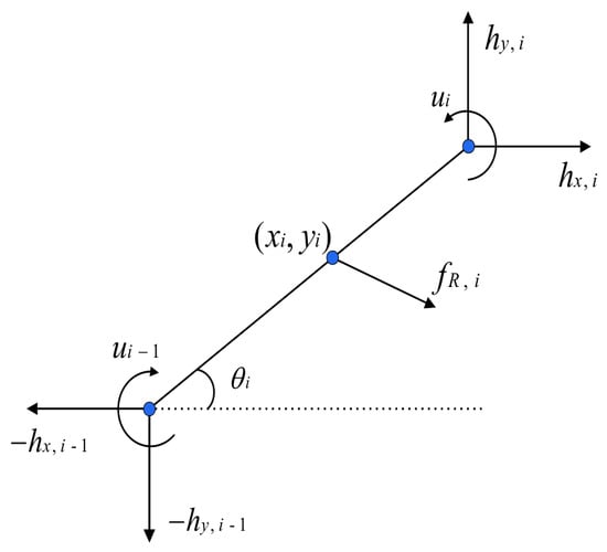
The mathematical model of the snake robot represents the system as a multi-link structure comprising N links interconnected by $N-1$ joints. Each link is assumed to be identical, having equal mass, rotational inertia, shape, and density, as shown in Figure 1. The dotted horizontal line indicates the reference direction, the global x-axis, from which the link orientation angle ${\theta }_i$ is measured. This modular idealization simplifies the model and isolates the effect of the control law. Additionally, the density of each link in the snake robot is uniformly distributed, with no variations across different parts of the link. The subsequent calculations will utilize the following parameter matrix.

Figure 1. The force analysis of the connecting rod.

The matrices A and D represent the sums and differences of quantities across adjacent links, respectively. The dimensionless vector e is the N-dimensional vector of ones. Left-multiplying by $e^{\top }$ yields the sum of a quantity across all links, whereas multiplying a scalar by e distributes that scalar uniformly across all links. In particular, $De=0$ and $e^{\top }e=N$. The block matrix E generalizes these summation and distribution properties to the two Cartesian coordinate directions.

$$\begin{array}{cc}\hfill A& :=\left[\begin{array}{ccccc}1& 1& & & \\ & .& .& & \\ & & .& .& \\ & & & 1& 1\end{array}\right]\in {\mathbb{R}}^{(N-1)\times N},D:=\left[\begin{array}{ccccc}1& -1& & & \\ & .& .& & \\ & & .& .& \\ & & & 1& -1\end{array}\right]\in {\mathbb{R}}^{(N-1)\times N},\hfill \\ \hfill e& :={[1,\cdots ,1]}^{\top }\in {\mathbb{R}}^N,E:=\left[\begin{array}{cc}e& 0_{N\times 1}\\ 0_{N\times 1}& e\end{array}\right]\in {\mathbb{R}}^{2N\times 2},\theta :={[{\theta }_1,\cdots ,{\theta }_N]}^{\top }\in {\mathbb{R}}^N,\hfill \\ \hfill \sin \theta & :={[\sin {\theta }_1,\cdots ,\sin {\theta }_N]}^{\top }\in {\mathbb{R}}^N,S_{\theta }:=\mathrm{diag}\left(\sin \theta \right)\in {\mathbb{R}}^{N\times N},\hfill \\ \hfill \cos \theta & :={[\cos {\theta }_1,\cdots ,\cos {\theta }_N]}^{\top }\in {\mathbb{R}}^N,C_{\theta }:=\mathrm{diag}\left(\cos \theta \right)\in {\mathbb{R}}^{N\times N},\hfill \\ \hfill \mathrm{sgn}\theta & :={[\mathrm{sgn}{\theta }_1,\cdots ,\mathrm{sgn}{\theta }_N]}^{\top }\in {\mathbb{R}}^N,{\dot{\theta }}^2:={[{\dot{\theta }}_1^2,\cdots ,{\dot{\theta }}_N^2]}^{\top }\in {\mathbb{R}}^N.\hfill \end{array}$$

(1)

The relative joint angles are defined from the global link orientations ${\theta }_i$ as

$${\varphi }_i:={\theta }_i-{\theta }_{i+1},i=1,2,\dots ,N-1.$$

(2)

A serpentine motion within the plane can be achieved at any position of the link, utilizing the previously defined coordinate system. When the link angle is denoted as ${\theta }_i$, the transformation matrix between the link and the world coordinate system is represented as

$$R_i^{\mathrm{Global}}:=\left[\begin{array}{cc}\cos {\theta }_i& -\sin {\theta }_i\\ \sin {\theta }_i& \cos {\theta }_i\end{array}\right].$$

(3)

The centroid coordinates are given by

$$X:={[x_1,\dots ,x_N]}^{\top },Y:={[y_1,\dots ,y_N]}^{\top },p:=\left[\begin{array}{c}{p}_x\\ p_y\end{array}\right]=\left[\begin{array}{c}{\displaystyle \frac{1}{Nm}}{\displaystyle {\sum }_{i=1}^N}m{x}_i\\ {\displaystyle \frac{1}{Nm}}{\displaystyle {\sum }_{i=1}^N}m{y}_i\end{array}\right]={\displaystyle \frac{1}{N}}\left[\begin{array}{c}{e}^{T}X\\ e^{T}Y\end{array}\right],$$

(4)

where X and Y denote the coordinate set of all connecting rod centroids, $p_x$ and $p_y$ represent the global coordinates of the centroid of the snake robot.

The coordinate relationship between the links can be derived

$$\begin{array}{cc}\hfill x_{i+1}-x_i& =l\cos \left({\theta }_i\right)+l\cos \left({\theta }_{i+1}\right),y_{i+1}-y_i=l\sin \left({\theta }_i\right)+l\sin \left({\theta }_{i+1}\right).\hfill \end{array}$$

(5)

Furthermore, the matrix form of the coordinate equations can be obtained

$$\begin{array}{ccc}\hfill DX+lA\cos \theta & =0,DY+lA\sin \theta \hfill & \hfill =0.\end{array}$$

(6)

The coordinate equations and the centroid equations are expressed in a compact form as follows:

$$\begin{array}{cc}\hfill TX& =\left[\begin{array}{c}-lA\cos \left(\theta \right)\\ p_x\end{array}\right],TY=\left[\begin{array}{c}-lA\sin \left(\theta \right)\\ p_y\end{array}\right],\hfill \end{array}$$

(7)

where $T:=\left[\begin{array}{c}D\\ {\displaystyle \frac{1}{N}}{e}^{\top }\end{array}\right]\in {\mathbb{R}}^{N\times N}$. Because D has rank $N-1$ and its null space is spanned by e, augmenting D with ${\displaystyle \frac{e^T}{N}}$ yields a nonsingular matrix T.

$$T^{-1}=\left[\begin{array}{cc}{D}^{\top }{\left(D{D}^{\top }\right)}^{-1}& e\end{array}\right].$$

(8)

Then, the coordinates of the links can be obtained by

$$\begin{array}{cc}\hfill X& =T^{-1}\left[\begin{array}{c}-lA\cos \theta \\ p_x\end{array}\right]=-l{K}^{\top }\cos \theta +e{p}_x,Y=T^{-1}\left[\begin{array}{c}-lA\sin \theta \\ p_y\end{array}\right]=-l{K}^{\top }\sin \theta +e{p}_y,\hfill \end{array}$$

(9)

where $K^{\top }:=D^{\top }{\left(D{D}^{\top }\right)}^{-1}A\in {\mathbb{R}}^{N\times N}$. Since $e^{\top }{K}^{\top }=0$, the vectors $-l{K}^{\top }\cos \theta$ and $-l{K}^{\top }\sin \theta$ describe the link-center positions relative to the robot’s center of mass. The terms $e{p}_x$ and $e{p}_y$ add the same center-of-mass translation to all links.

Taking the derivatives of (9), we have

$$\begin{array}{cc}\hfill \dot{X}& =l{K}^{\top }{S}_{\theta }\dot{\theta }+e{\dot{p}}_x,\dot{Y}=-l{K}^{\top }{C}_{\theta }\dot{\theta }+e{\dot{p}}_y.\hfill \end{array}$$

(10)

Expanding the above equations, we obtain the corresponding velocities as follows

$$\begin{array}{cc}\hfill {\dot{x}}_i& ={\dot{p}}_x-{\sigma }_i{S}_{\theta }\dot{\theta },{\dot{y}}_i={\dot{p}}_y+{\sigma }_i{C}_{\theta }\dot{\theta },\hfill \end{array}$$

(11)

where ${\sigma }_i:=-l{\left[K^{\top }\right]}_{i,:}\in {\mathbb{R}}^{1\times N}$, ${\left[K^{\top }\right]}_{i,:}$ denotes the i-th row of the matrix.

Furthermore, taking the derivatives of (11) yields $\ddot{x_i}$ and $\ddot{y_i}$. With free endpoints, the robot has zero endpoint constraint forces, i.e., $h_{x,0}=h_{y,0}=h_{x,N}=h_{y,N}=0$. By conducting force analysis on the links, we can obtain the force equations of the links as

$$\begin{array}{cc}\hfill m\ddot{x_i}& =f_{R,x,i}+h_{x,i}-h_{x,i-1},m\ddot{y_i}=f_{R,y,i}+h_{y,i}-h_{y,i-1},i=1,\dots ,N,\hfill \end{array}$$

(12)

where $(h_{x,i},h_{y,i})$ denotes the joint constraint force exerted by link $i+1$ on link i, whereas $-(h_{x,i-1},h_{y,i-1})$ denotes the joint constraint force exerted by link $i-1$ on link i. The link force balances can be written in matrix form as

$$\begin{array}{cc}\hfill m\ddot{X}& =f_{R,x}+D^{\top }{h}_x,m\ddot{Y}=f_{R,y}+D^{\top }{h}_y,\hfill \end{array}$$

(13)

here,

$$\begin{array}{ccc}\hfill & h_x:={[h_{x,1},h_{x,2},\dots ,h_{x,N-1}]}^{\top },\hfill & \hfill h_y:={[h_{y,1},h_{y,2},\dots ,h_{y,N-1}]}^{\top }.\end{array}$$

(14)

By further differentiation, we get

$$\begin{array}{c}\hfill D\ddot{X}=lA\left(C_{\theta }{\dot{\theta }}^2+S_{\theta }\ddot{\theta }\right),D\ddot{Y}=lA\left(S_{\theta }{\dot{\theta }}^2-C_{\theta }\ddot{\theta }\right).\end{array}$$

(15)

Premultiplying the link force balances in (13) by $e^{\top }$ sums the forces acting on all links. Since $e^{\top }{D}^{\top }=0$, the joint constraint forces cancel, leaving the net external ground-friction force. Together with the equal-mass center-of-mass relation in (4), this yields

$$\left[\begin{array}{c}\ddot{p_x}\\ \ddot{p_y}\end{array}\right]={\displaystyle \frac{1}{N}}\left[\begin{array}{c}{e}^{\top }\ddot{X}\\ e^{\top }\ddot{Y}\end{array}\right]={\displaystyle \frac{1}{Nm}}\left[\begin{array}{c}{e}^{\top }{f}_{R,x}\\ e^{\top }{f}_{R,y}\end{array}\right].$$

(16)

Following the modeling assumption of Mohammadi et al. [43], the interaction between each link and the ground is modeled with an anisotropic linear viscous friction model. The ground friction forces are external contact forces determined by the link velocities and orientations, whereas the actuator torques are the physical control inputs. Transforming the local friction law into the global coordinate frame yields

$$\begin{array}{cc}\hfill f_{R,i}& =-\left[\begin{array}{cc}\cos {\theta }_i& -\sin {\theta }_i\\ \sin {\theta }_i& \cos {\theta }_i\end{array}\right]\left[\begin{array}{cc}{c}_t& 0\\ 0& c_n\end{array}\right]{\left[\begin{array}{cc}\cos {\theta }_i& -\sin {\theta }_i\\ \sin {\theta }_i& \cos {\theta }_i\end{array}\right]}^{\top }\left[\begin{array}{c}\dot{x_i}\\ \dot{y_i}\end{array}\right].\hfill \end{array}$$

(17)

The constants $c_t$ and $c_n$ are the tangential and transverse viscous friction coefficients, respectively, with units of $\mathrm{N}·\mathrm{s}·{\mathrm{m}}^{-1}$. The assumption $c_n>c_t>0$ implies greater resistance to transverse motion than to tangential motion at the same speed. The interaction between this directional resistance and cyclic changes in body shape enables net locomotion. Under this velocity-dependent law, the friction force on a stationary link is zero; static friction, transitions between sticking and sliding, and anchoring by spikes or setae are therefore excluded from this model. The friction forces for all links can be written in compact form as

$$\begin{array}{cc}\hfill f_R& =-\left[\begin{array}{cc}{c}_t{\left(C_{\theta }\right)}^2+c_n{\left(S_{\theta }\right)}^2& (c_t-c_n)S_{\theta }{C}_{\theta }\\ (c_t-c_n)S_{\theta }{C}_{\theta }& c_t{\left(S_{\theta }\right)}^2+c_n{\left(C_{\theta }\right)}^2\end{array}\right]\left[\begin{array}{c}\dot{X}\\ \dot{Y}\end{array}\right]\in {\mathbb{R}}^{2N}.\hfill \end{array}$$

(18)

The endpoint torques are defined as $u_0:=0,u_N:=0$ because the actuators are located only at the $N-1$ internal joints. Based on the force analysis of the links from Figure 1, the total torque can be expressed as

$$\begin{array}{cc}\hfill J\ddot{{\theta }_i}& =u_i-u_{i-1}-l\sin \left({\theta }_i\right)\left(h_{x,i}+h_{x,i-1}\right)+l\cos \left({\theta }_i\right)\left(h_{y,i}+h_{y,i-1}\right),i=1,\dots ,N,\hfill \end{array}$$

(19)

where, $u_i$ represents the actuator torque of joint i, exerting $u_i$ and $-u_i$ on links i and $i+1$, respectively. Then, we have $u:={[u_1,\dots ,u_{N-1}]}^{\top }\in {\mathbb{R}}^{N-1}$. Furthermore, we obtain

$$J\ddot{\theta }=D^{\top }u-l{S}_{\theta }{A}^{\top }{h}_x+l{C}_{\theta }{A}^{\top }{h}_y.$$

(20)

Multiplying Equations (13) by matrix D yields

$$\begin{array}{c}\hfill mD\ddot{X}=D{f}_{R,x}+D{D}^{\top }{h}_x,mD\ddot{Y}=D{f}_{R,y}+D{D}^{\top }{h}_y.\end{array}$$

(21)

Eliminating the joint constraint forces using (15), (20), and (21), we obtain

$$M_{\theta }\ddot{\theta }+W{\dot{\theta }}^2-l{S}_{\theta }K{f}_{R,x}+l{C}_{\theta }K{f}_{R,y}=D^{\top }u,$$

(22)

$$\ddot{p}={\displaystyle \frac{1}{Nm}}\left[\begin{array}{c}{e}^{\top }{f}_{R,x}\\ e^{\top }{f}_{R,y}\end{array}\right],$$

(23)

$$\begin{array}{cc}\hfill & M_{\theta }:=J{I}_N+m{l}^2{S}_{\theta }V{S}_{\theta }+m{l}^2{C}_{\theta }V{C}_{\theta },\hfill \\ \hfill & W:=m{l}^2\left(S_{\theta }V{C}_{\theta }-C_{\theta }V{S}_{\theta }\right),\hfill \\ \hfill & V:=A^{\top }{\left(D{D}^{\top }\right)}^{-1}A,K:=A^{\top }{\left(D{D}^{\top }\right)}^{-1}D,\hfill \end{array}$$

(24)

here, the notation $I_d$ denotes the $d\times d$ identity matrix, $M_{\theta }\left(\theta \right)\in {\mathbb{R}}^{N\times N}$ is the inertia matrix in the global link-angle coordinates, and $W\left(\theta \right)\in {\mathbb{R}}^{N\times N}$ contains the coefficients of the quadratic velocity term. The constant matrices $V,K\in {\mathbb{R}}^{N\times N}$ are determined by the link-connectivity matrices A and D.

Remark 1.

The analysis above shows that the snake robot behaves as a high-order nonlinear system, as evidenced by the squared term involving the first-order derivative of the link angle θ in Equation (22). Furthermore, the input u represents the torque applied by the joints to the links. The robot has $N+2$ generalized coordinates and $N-1$ independent joint torques, resulting in three degrees of underactuation [43]. The head-link orientation and center-of-mass position are not directly actuated. Nevertheless, joint motion changes the distributed ground friction, coupling the actuated and unactuated dynamics and enabling indirect control of locomotion.

Define the matrix H to correlate the joint angle and the link angle

$$\begin{array}{cc}\hfill H& :=\left[\begin{array}{cccccc}1& 1& 1& \cdots & 1& 1\\ 0& 1& 1& \cdots & 1& 1\\ ⋮& & & & & ⋮\\ 0& 0& 0& \cdots & 0& 1\end{array}\right]\in {\mathbb{R}}^{N\times N}.\hfill \end{array}$$

(25)

Consider defining the generalized-coordinate vector $q_{\varphi }$ as the set of the joint angle, snake head link angle, and centroid

$$\begin{array}{c}\hfill q_{\varphi }:=\left[\begin{array}{c}\overline{\varphi }\\ p\end{array}\right]\in {\mathbb{R}}^{N+2},\end{array}$$

(26)

where $\overline{\varphi }:={[{\varphi }_1,{\varphi }_2,\dots ,{\varphi }_{N-1},{\theta }_N]}^{\top }$, and p represents the centroid of the snake robot. The relationship between $\overline{\varphi }$ and $\theta$ can be computed using matrix H

$$\begin{array}{c}\hfill \theta =H\overline{\varphi }.\end{array}$$

(27)

Substituting Equation (27) into Equation (22), we obtain

$$\begin{array}{c}\hfill M_{\theta }H\ddot{\overline{\varphi }}+W\mathrm{diag}\left(H\dot{\overline{\varphi }}\right)H\dot{\overline{\varphi }}-l{S}_{\theta }K{f}_{R,x}+l{C}_{\theta }K{f}_{R,y}=D^{\top }u.\end{array}$$

(28)

Define the actuated and unactuated coordinate vectors as $q_a:={[{\varphi }_1,{\varphi }_2,\dots ,{\varphi }_{N-1}]}^{\top }\in {\mathbb{R}}^{N-1},q_u:={[{\theta }_N,p_x,p_y]}^{\top }\in {\mathbb{R}}^3$, so that $q_{\varphi }={[q_a^{\top },q_u^{\top }]}^{\top }$. The relation ${\displaystyle \left[\begin{array}{c}\theta \\ p\end{array}\right]:=\left[\begin{array}{cc}H& 0_{N\times 2}\\ 0_{2\times N}& I_2\end{array}\right]q_{\varphi }}$ defines an invertible linear change of generalized coordinates, since H is upper triangular with unit diagonal. Premultiplication of the rotational dynamics by $H^{\top }$ accounts for the corresponding transformation of generalized forces. Moreover, ${\displaystyle DH:=\left[\begin{array}{cc}{I}_{N-1}& 0_{(N-1)\times 1}\end{array}\right],H^{\top }{D}^{\top }:=\left[\begin{array}{c}{I}_{N-1}\\ 0_{1\times (N-1)}\end{array}\right].}$ Premultiplying (28) by $H^{\top }$, multiplying (23) by $Nm$, and partitioning the resulting equations according to the actuated and unactuated coordinates yields (29).

$$\begin{array}{cc}\hfill & \overline{M}:=\left[\begin{array}{cc}{H}^{\top }{M}_{\theta }H& 0_{N\times 2}\\ 0_{2\times N}& Nm{I}_2\end{array}\right],\overline{W}:=\left[\begin{array}{c}{H}^{\top }W{\dot{\theta }}^2\\ 0_{2\times 1}\end{array}\right],\overline{G}:=\left[\begin{array}{cc}-l{H}^{\top }{S}_{\theta }K& l{H}^{\top }{C}_{\theta }K\\ -e^{\top }& 0_{1\times N}\\ 0_{1\times N}& -e^{\top }\end{array}\right],\hfill \\ \hfill & \overline{M}:=\left[\begin{array}{cc}{\overline{M}}_{11}& {\overline{M}}_{12}\\ {\overline{M}}_{21}& {\overline{M}}_{22}\end{array}\right],\overline{W}:=\left[\begin{array}{c}{\overline{W}}_1\\ {\overline{W}}_2\end{array}\right],\overline{G}:=\left[\begin{array}{c}{\overline{G}}_1\\ {\overline{G}}_2\end{array}\right],\left\{\begin{array}{cc}\hfill {\overline{M}}_{11}{\ddot{q}}_a+{\overline{M}}_{12}{\ddot{q}}_u+{\overline{W}}_1+{\overline{G}}_1{f}_R& =u,\hfill \\ \hfill {\overline{M}}_{21}{\ddot{q}}_a+{\overline{M}}_{22}{\ddot{q}}_u+{\overline{W}}_2+{\overline{G}}_2{f}_R& =0_{3\times 1},\hfill \end{array}\right.\hfill \end{array}$$

(29)

where ${\overline{M}}_{11}\in {\mathbb{R}}^{N-1\times N-1},$ ${\overline{M}}_{12}\in {\mathbb{R}}^{N-1\times 3},$ ${\overline{M}}_{21}\in {\mathbb{R}}^{3\times N-1},$ ${\overline{M}}_{22}\in {\mathbb{R}}^{3\times 3},$ ${\overline{W}}_1\in {\mathbb{R}}^{N-1},$ ${\overline{W}}_2\in {\mathbb{R}}^3,$ ${\overline{G}}_1\in {\mathbb{R}}^{N-1\times 2N},$ ${\overline{G}}_2\in {\mathbb{R}}^{3\times 2N}$.

Equation (29) is the standard partitioned form of an underactuated mechanical system, $\overline{M}\left(q_{\varphi }\right){\ddot{q}}_{\varphi }+\overline{W}(q_{\varphi },{\dot{q}}_{\varphi })+\overline{G}\left(q_{\varphi }\right)f_R=Bu$, where $B=\left[\begin{array}{c}{I}_{N-1}\\ 0_{3\times (N-1)}\end{array}\right]$. For the physical parameters $J>0$ and $m>0$, $V=A^{\top }{\left(D{D}^{\top }\right)}^{-1}A⪰0$, which gives $M_{\theta }⪰J{I}_N$; since H is nonsingular, the transformed inertia matrix is symmetric positive definite. Moreover, because the last column of H is e, ${\overline{M}}_{22}=\mathrm{diag}(e^{\top }{M}_{\theta }e,Nm,Nm)$, and $e^{\top }{M}_{\theta }e\ge JN>0$. Therefore, ${\overline{M}}_{22}\succ 0$ and is consequently nonsingular.

Following the underactuated-system framework in [44], the joint dynamics can be partially linearized via state feedback. Input–output linearization of the joint dynamics is also employed in the snake-robot formulation of [43]. First, solving the unactuated equation in (29) for ${\ddot{q}}_u$ yields

$${\ddot{q}}_u=-{\overline{M}}_{22}^{-1}({\overline{M}}_{21}{\ddot{q}}_a+{\overline{W}}_2+{\overline{G}}_2{f}_R).$$

(30)

Substituting Equation (30) into the first equation of Equation (29) yields the following expression for the input torque u:

$$u=({\overline{M}}_{11}-{\overline{M}}_{12}{\overline{M}}_{22}^{-1}{\overline{M}}_{21}){\ddot{q}}_a+{\overline{W}}_1+{\overline{G}}_1{f}_R-{\overline{M}}_{12}{\overline{M}}_{22}^{-1}({\overline{W}}_2+{\overline{G}}_2{f}_R).$$

(31)

The vector $q_a$ contains the $N-1$ actuated joint angles, and ${\ddot{q}}_a$ denotes the corresponding angular accelerations. The desired joint accelerations are specified in the following section. The relationship between the unactuated coordinates $q_u$ and the actuated coordinates $q_a$ is then written as follows:

$${\ddot{q}}_u=U+Z{\ddot{q}}_a,$$

(32)

where $U:=-{\overline{M}}_{22}^{-1}({\overline{W}}_2+{\overline{G}}_2{f}_R),Z:=-{\overline{M}}_{22}^{-1}{\overline{M}}_{21}$.

With the expressions for the velocities and accelerations of the state variables $q_a$ and $q_u$ determined, we define the global state variable as

$$x:=\left[\begin{array}{c}{q}_a\\ q_u\\ {\dot{q}}_a\\ {\dot{q}}_u\end{array}\right]\in {\mathbb{R}}^{2N+4}.$$

(33)

Define the Schur complement $S:={\overline{M}}_{11}-{\overline{M}}_{12}{\overline{M}}_{22}^{-1}{\overline{M}}_{21}$. Since $\overline{M}$ is symmetric positive definite, S is also symmetric positive definite. Replacing ${\ddot{q}}_a$ in the torque law (31) with the virtual input $\overline{u}$ therefore defines a smooth, invertible static state-feedback transformation with respect to $\overline{u}$. This transformation is termed collocated partial feedback linearization because the linearized coordinates are the actuated joint coordinates. It yields ${\ddot{q}}_a=\overline{u},{\ddot{q}}_u=U+Z\overline{u}$. The joint subsystem consequently consists of $N-1$ double integrators, while the unactuated dynamics retain their nonlinear dependence on the state. The corresponding first-order representation is

$$\dot{x}=\left[\begin{array}{c}{\dot{q}}_a\\ {\dot{q}}_u\\ \overline{u}\\ U+Z\overline{u}\end{array}\right].$$

(34)

3. Controller Design Based on Backstepping and Virtual Holonomic Constraints

Most control method designs in this study are model-based. Therefore, it is essential to thoroughly analyze and study the model of the research subject. In the design of control methods, common techniques such as backstepping and Lyapunov-based analysis are used to construct virtual controls and assess closed-loop stability [45]. Another approach involves controlling nonlinear systems through methods like local feedback linearization. These two methods are implemented in this paper to achieve dynamic control of the snake robot. Before delving into the control method design, the challenges faced by the control system are considered. First and foremost, the joint tracking problem is addressed, with a focus on achieving precise tracking of the given time-varying joint angles. Subsequently, the system’s velocity control problem is examined, involving the generation of target joint angles based on expected velocities and the model. Furthermore, the paper considers the path tracking and path planning problems. However, due to scope limitations, the focus is solely on the path tracking problem.

Within the Euler–Lagrange framework, virtual holonomic constraints can define a lower-dimensional invariant manifold for control design [46]. In the present snake-robot model, introducing VHCs enables the construction of the corresponding reduced state equations, following the snake-robot application in [43]. Based on these considerations, this section is divided into two parts: one focuses on straight-line tracking, and the other focuses on curved-path tracking.

For periodic locomotion, averaging methods and vibrational-mechanics approaches are established tools for deriving slow dynamics from rapidly oscillating systems [47,48]. In this study, the gait is prescribed directly via the VHC parameterization in (35). In this section, the joint angle variations discussed follow the form

$$\begin{array}{c}\hfill {\varphi }_{i,\mathrm{ref}}:=\alpha \sin \left(\lambda +(i-1)\delta \right)+b_i{\varphi }_0,i=1,2,\dots ,N-1,\end{array}$$

(35)

where $\alpha$ is the joint-angle amplitude, $\delta$ is the phase difference between adjacent joints, $\lambda$ is the time-varying gait phase, ${\varphi }_0$ is a time-varying joint-angle offset. The vector $b:={[0,\dots ,0,1]}^{\top }\in {\mathbb{R}}^{N-1}$ specifies how the offset is distributed among the joints, and $b_i$ denotes its i-th component. The first question to address is the ideal virtual joint-acceleration input $\overline{u}$.

Considering the previous definitions of link angles and joint angles, we introduce the actual joint angles as

$$\begin{array}{cc}\hfill \varphi & :={[{\varphi }_1,\dots ,{\varphi }_{N-1}]}^{\top }=D\theta \in {\mathbb{R}}^{N-1}.\hfill \end{array}$$

(36)

Following the VHC formulation of [43,46], we have ${\Phi }_i\left(\lambda \right):=\alpha \sin [\lambda +(i-1)\delta ],\Phi \left(\lambda \right)={[{\Phi }_1\left(\lambda \right),\dots ,{\Phi }_{N-1}\left(\lambda \right)]}^{\top }$. In addition, we define ${\varphi }_{\mathrm{ref}}:={[{\varphi }_{1,\mathrm{ref}},\dots ,{\varphi }_{N-1,\mathrm{ref}}]}^{\top }=\Phi \left(\lambda \right)+b{\varphi }_0$. To ensure that the joint angle input under ideal conditions matches the expected target joint angles, considering the time-varying nature of the joint angles, the desired joint angle’s acceleration is given by

$$\begin{array}{c}\hfill \overline{u}:={\ddot{\varphi }}_{\mathrm{ref}}+K_d({\dot{\varphi }}_{\mathrm{ref}}-\dot{\varphi })+K_p({\varphi }_{\mathrm{ref}}-\varphi ).\end{array}$$

(37)

where the matrices $K_p,K_d\in {\mathbb{R}}^{(N-1)\times (N-1)}$ are constant positive definite diagonal matrices specifying the joint-position and joint-velocity feedback gains, respectively. However, $\overline{u}$ cannot be directly used as the joint torque input to the system. To transform Equation (22), first, both sides of the equation are multiplied by $M_{\theta }^{-1}$ to obtain

$$\begin{array}{cc}\hfill \ddot{\theta }+M_{\theta }^{-1}W{\dot{\theta }}^2-l{M}_{\theta }^{-1}{S}_{\theta }K{f}_{R,x}+l{M}_{\theta }^{-1}{C}_{\theta }K{f}_{R,y}& =M_{\theta }^{-1}{D}^{\top }u.\hfill \end{array}$$

(38)

Once the actual joint angles and the desired joint angles are defined, the tracking error is defined as

$$\begin{array}{c}\hfill z:=\varphi -{\varphi }_{\mathrm{ref}}=D\theta -\Phi \left(\lambda \right)-b{\varphi }_0,\end{array}$$

(39)

when the error z approaches 0, the tracking of $\varphi$ is accomplished. Multiplying Equation (38) on the left by the matrix D, we get

$$\begin{array}{cc}\hfill \ddot{\varphi }+D{M}_{\theta }^{-1}W{\dot{\theta }}^2-lD{M}_{\theta }^{-1}{S}_{\theta }K{f}_{R,x}+lD{M}_{\theta }^{-1}{C}_{\theta }K{f}_{R,y}& =D{M}_{\theta }^{-1}{D}^{\top }u.\hfill \end{array}$$

(40)

Knowing that $\overline{u}=\ddot{\varphi }$, the joint torque to be applied is obtained as

$$\begin{array}{cc}\hfill u& ={\left(D{M}_{\theta }^{-1}{D}^{\top }\right)}^{-1}(D{M}_{\theta }^{-1}W{\dot{\theta }}^2-lD{M}_{\theta }^{-1}S{C}_{\theta }^{\top }{f}_R+\overline{u}),\hfill \end{array}$$

(41)

where $S{C}_{\theta }:=\left[\begin{array}{c}{K}^{\top }{S}_{\theta }\\ -K^{\top }{C}_{\theta }\end{array}\right]\in {\mathbb{R}}^{2N\times N}$. Since this joint controller is based on the snake robot’s dynamic model, it ensures that the joints can track the given joint angles (35) and completes the design of the joint controller.

The compensator states $\lambda$ and ${\varphi }_0$ are used for speed and heading regulation, respectively. To obtain the unactuated rotational equation, we premultiply (22) by $e^{\top }$. Since $De=0$, the vector e represents a common angular variation of all links that leaves the relative joint angles unchanged. Consequently, $e^{\top }{D}^{\top }u=0$, indicating cancellation of the internal actuator torques. After eliminating the interlink constraint forces, the projected equation represents the angular-momentum balance about the robot’s center of mass and retains the external ground-friction moment:

$$\begin{array}{c}\hfill e^{\top }{M}_{\theta }\ddot{\theta }+e^{\top }W{\dot{\theta }}^2-l{e}^{\top }S{C}_{\theta }^{\top }{f}_R=0.\end{array}$$

(42)

Considering the geometric relationship between joint angles and link angles, as shown in Figure 1, the relationship between link angles and joint angles can be derived as

$$\begin{array}{c}\hfill \theta =H_{a}D\theta +e{\theta }_N,\end{array}$$

(43)

where $H_{\mathrm{a}}:=\left[\begin{array}{cccc}1& 1& \cdots & 1\\ 0& 1& \cdots & 1\\ ⋮& & & ⋮\\ 0& 0& \cdots & 1\\ 0& 0& \cdots & 0\end{array}\right]\in {\mathbb{R}}^{N\times (N-1)}$, which consists of the first $N-1$ columns of H.

On the invariant VHC manifold defined by $z=0$ and $\dot{z}=0$, the joint configuration satisfies

$$\begin{array}{cc}\hfill D\theta & =\Phi \left(\lambda \right)+b{\varphi }_0.\hfill \end{array}$$

(44)

Substituting (44) into (43), we obtain

$$\begin{array}{cc}\hfill \theta & =H_a\Phi \left(\lambda \right)+H_{a}b{\varphi }_0+e{\theta }_N.\hfill \end{array}$$

(45)

On the invariant VHC manifold, the reduced dynamics are described by the five coordinates $\lambda ,{\varphi }_0,{\theta }_N,p_x,p_y$ and their first time derivatives, giving a ten-dimensional state. By substituting (45) into (42), we have $e^T{M}_{\theta }\ddot{\theta }=e^T{M}_{\theta }{H}_a{\Phi }^{″}\left(\lambda \right){\dot{\lambda }}^2+e^T{M}_{\theta }{H}_a{\Phi }^{\prime }\left(\lambda \right)\ddot{\lambda }+e^T{M}_{\theta }{H}_{a}b{\ddot{\varphi }}_0+e^T{M}_{\theta }e{\ddot{\theta }}_N$. By defining $e^{\top }{M}_{\theta }{H}_a{\Phi }^{″}\left(\lambda \right)={\overline{M}}_{\theta 1}$, $e^{\top }{M}_{\theta }{H}_a{\Phi }^{\prime }\left(\lambda \right)={\overline{M}}_{\theta 2}$, $e^{\top }{M}_{\theta }{H}_{a}b={\overline{M}}_{\theta 3}$, and $e^{\top }{M}_{\theta }e={\overline{M}}_{\theta 4}$, we can derive the expression for ${\ddot{\theta }}_N$:

$${\ddot{\theta }}_N=-{\displaystyle \frac{{\overline{M}}_{\theta 1}}{{\overline{M}}_{\theta 4}}}{\dot{\lambda }}^2-{\displaystyle \frac{{\overline{M}}_{\theta 2}}{{\overline{M}}_{\theta 4}}}\ddot{\lambda }-{\displaystyle \frac{{\overline{M}}_{\theta 3}}{{\overline{M}}_{\theta 4}}}{\ddot{\varphi }}_0-{\displaystyle \frac{e^{\top }W}{{\overline{M}}_{\theta 4}}}{\dot{\theta }}^2+{\displaystyle \frac{l{e}^{T}S{C}_{\theta }^{\top }}{{\overline{M}}_{\theta 4}}}{f}_R,$$

(46)

where $\ddot{\lambda }=u_{\lambda },{\ddot{\varphi }}_0=u_{{\varphi }_0},\ddot{p}={\displaystyle \frac{1}{Nm}}\left[\begin{array}{c}{e}^{\top }{f}_{R,x}\\ e^{\top }{f}_{R,y}\end{array}\right]$. The scalar virtual inputs $u_{\lambda }$ and $u_{{\varphi }_0}$ prescribe the accelerations of the gait phase and steering offset, respectively. Then we derive the dynamical model of the snake robot after applying the VHC method.

To control the motion of the snake robot, we set the desired head-link heading as ${\theta }_{ref}$ and its first and second derivatives as ${\dot{\theta }}_{ref}$ and ${\ddot{\theta }}_{ref}$, respectively, with the constant desired tangential velocity as $v_{ref}$. Next, we address the direction and velocity tracking problems of the snake robot sequentially.

Firstly, we address the direction tracking problem. From Equation (46), we observe the part related to ${\ddot{\varphi }}_0$. To ensure convergence in subsequent calculations, we use the following control input for ${\ddot{\varphi }}_0$.

$$\begin{array}{c}\hfill u_{{\varphi }_0}:={\displaystyle \frac{{\overline{M}}_{\theta 4}}{{\overline{M}}_{\theta 3}}}{u}_{p1}({\dot{\theta }}_e+u_{p2}{\theta }_e)-u_{p3}{\varphi }_0-u_{p4}\left({\dot{\varphi }}_0+u_{p5}\sin \left(\dot{\lambda }\right)\right),\end{array}$$

(47)

where ${\theta }_e:={\theta }_N-{\theta }_{ref}$. The constants $u_{p1}$ and $u_{p2}$ determine the heading-feedback strength and the reduced heading-error convergence rate, respectively. The constants $u_{p3}$ and $u_{p4}$ provide restoring and damping feedback for the steering-offset dynamics, while $u_{p5}$ scales the phase-rate-dependent term. The operating domain excludes zeros of ${\overline{M}}_{\theta 3}$. The arguments of the phase-rate sine terms use $\dot{\lambda }$ normalized by $1\mathrm{rad}{\mathrm{s}}^{-1}$. Differentiating the heading error twice with respect to time gives

$$\begin{array}{c}\hfill {\ddot{\theta }}_e={\ddot{\theta }}_N-{\ddot{\theta }}_{ref}.\end{array}$$

(48)

To calculate the formulas related to $u_{{\varphi }_0}$ independently, we transform ${\ddot{\theta }}_N$ in Equation (46) into the following form

$$\begin{array}{c}\hfill {\ddot{\theta }}_N={\Theta }_{p1}-{\displaystyle \frac{{\overline{M}}_{\theta 3}}{{\overline{M}}_{\theta 4}}}{\ddot{\varphi }}_0,\end{array}$$

(49)

where ${\Theta }_{p1}:=-{\displaystyle \frac{{\overline{M}}_{\theta 1}}{{\overline{M}}_{\theta 4}}}{\dot{\lambda }}^2-{\displaystyle \frac{{\overline{M}}_{\theta 2}}{{\overline{M}}_{\theta 4}}}\ddot{\lambda }-{\displaystyle \frac{e^{T}W}{{\overline{M}}_{\theta 4}}}{\dot{\theta }}^2+{\displaystyle \frac{l{e}^{T}S{C}_{\theta }^{\top }}{{\overline{M}}_{\theta 4}}}{f}_R$. Substituting (47) into (49), we obtain

$$\begin{array}{c}\hfill {\ddot{\theta }}_N={\Theta }_{p1}-u_{p1}\left({\dot{\theta }}_e+u_{p2}{\theta }_e\right)+{\displaystyle \frac{{\overline{M}}_{\theta 3}}{{\overline{M}}_{\theta 4}}}\left(u_{p3}{\varphi }_0+u_{p4}\left({\dot{\varphi }}_0+u_{p5}\sin \left(\dot{\lambda }\right)\right)\right),\end{array}$$

(50)

Define the positive singular perturbation parameter as $ϵ:={\displaystyle \frac{1}{u_{p1}}}$; the perturbation system of variable (50) is derived as follows:

$$\begin{array}{c}\hfill ϵ{\ddot{\theta }}_e=ϵ\left({\Theta }_{p1}-{\ddot{\theta }}_{\mathrm{ref}}+{\displaystyle \frac{{\overline{M}}_{\theta 3}}{{\overline{M}}_{\theta 4}}}\left(u_{p3}{\varphi }_0+u_{p4}\left({\dot{\varphi }}_0+u_{p5}\sin \left(\dot{\lambda }\right)\right)\right)\right)-\widehat{y},\end{array}$$

(51)

where $\widehat{y}:={\dot{\theta }}_e+u_{p2}{\theta }_e$ is the fast error coordinate. In the reduced system used for the singular-perturbation analysis, this coordinate is set to zero, i.e., $\widehat{y}={\dot{\theta }}_e+u_{p2}{\theta }_e=0$, by setting $ϵ=0$ in (51). For finite $ϵ>0$, $\widehat{y}$ remains a dynamic state and is retained in $V_1$.

The small parameter $ϵ={\displaystyle \frac{1}{u_{p1}}}$ is introduced by the heading-feedback gain. The time-scale separation therefore follows from the controller structure rather than the low locomotion speed alone [45,49]. The following estimates assume smooth reduced dynamics on the considered operating domain and a uniformly bounded coupling residual as $ϵ$ decreases.

In order to separately analyze $\widehat{y}$, the time-scale separation principle is applied to distinguish the perturbation term from the singular perturbation system. According to the boundary-layer principle, the system satisfies

$$\begin{array}{cc}\hfill {\displaystyle \frac{\mathrm{d}\widehat{y}}{\mathrm{d}\tau }}& =-\widehat{y},\hfill \end{array}$$

(52)

where $\tau ={\displaystyle \frac{t}{ϵ}}$. This equilibrium is exponentially stable. For $u_{p2}>0$, the reduced heading-error dynamics ${\dot{\theta }}_e=-u_{p2}{\theta }_e$ are exponentially stable. Under the hypotheses of Theorem 11.2 in [45], the following singular-perturbation estimates are obtained:

$$\begin{array}{c}\hfill {\theta }_e\left(t,ϵ\right)-e^{-u_{p2}t}{\theta }_e\left(0\right)=O\left(ϵ\right),\end{array}$$

(53)

$$\begin{array}{c}\hfill \dot{{\theta }_e}\left(t,ϵ\right)+u_{p2}{e}^{-u_{p2}t}{\theta }_e\left(0\right)-e^{-{\displaystyle \frac{t}{ϵ}}}{\widehat{y}}_0=O\left(ϵ\right).\end{array}$$

(54)

The initial time is set to $t=0$, with ${\widehat{y}}_0:=\widehat{y}\left(0\right):={\dot{\theta }}_e\left(0\right)+u_{p2}{\theta }_e\left(0\right)$. The notation $O\left(ϵ\right)$ denotes a remainder whose magnitude is bounded by a constant multiple of $ϵ$ for sufficiently small $ϵ$.

To analyze the heading-error dynamics, consider the following Lyapunov function candidate:

$$\begin{array}{c}\hfill V_1:={\displaystyle \frac{{\theta }_e^2}{2}}+{\displaystyle \frac{{\widehat{y}}^2}{2}}.\end{array}$$

(55)

Using (51) and the definition of $\widehat{y}$, the heading-error components of the closed-loop vector field can be written as ${\dot{\theta }}_e=\widehat{y}-u_{p2}{\theta }_e,\dot{\widehat{y}}=-{\displaystyle \frac{\widehat{y}}{ϵ}}+{\Theta }_{p1}-{\ddot{\theta }}_{\mathrm{ref}}+u_{p2}(\widehat{y}-u_{p2}{\theta }_e)+{\displaystyle \frac{{\overline{M}}_{\theta 3}}{{\overline{M}}_{\theta 4}}}\left[u_{p3}{\varphi }_0+u_{p4}\left({\dot{\varphi }}_0+u_{p5}\sin \left(\dot{\lambda }\right)\right)\right].$ Since $V_1$ depends only on ${\theta }_e$ and $\widehat{y}$, its derivative along the closed-loop vector field is

$$\begin{array}{cc}\hfill {\dot{V}}_1& ={\displaystyle \frac{\partial V_1}{\partial {\theta }_e}}{\dot{\theta }}_e+{\displaystyle \frac{\partial V_1}{\partial \widehat{y}}}\dot{\widehat{y}}\hfill \\ \hfill & ={\theta }_e(\widehat{y}-u_{p2}{\theta }_e)+\widehat{y}\dot{\widehat{y}}\hfill \\ \hfill & ={\theta }_e\widehat{y}-u_{p2}{\theta }_e^2+\widehat{y}\dot{\widehat{y}}.\hfill \end{array}$$

(56)

Denote all terms after $-{\displaystyle \frac{\widehat{y}}{ϵ}}$ in the expression for $\dot{\widehat{y}}$ by $R\left(t\right)$. Assume forward-complete trajectories in the considered operating domain and $\left|R\right(t\left)\right|\le L$ for a finite constant $L\ge 0$, uniformly over initial conditions in a neighborhood of the error set. In the singular limit considered here, the reduced relation is $\widehat{y}=0$; following the signed estimate used in the thesis derivation, $\widehat{y}\dot{\widehat{y}}\le -{\displaystyle \frac{{\widehat{y}}^2}{2ϵ}}+L\widehat{y}$, giving

$$\begin{array}{c}\hfill \dot{V_1}\le {\theta }_e\widehat{y}-u_{p2}{\theta }_e^2-{\displaystyle \frac{1}{2ϵ}}{\widehat{y}}^2+L\widehat{y}.\end{array}$$

(57)

The nonnegative sum of squares in (58) gives the inequality in (59):

$$\begin{array}{cc}\hfill {\left(\widehat{y}-{\theta }_e\right)}^2+{\left(\widehat{y}-L\right)}^2& \ge 0.\hfill \end{array}$$

(58)

$$\begin{array}{cc}\hfill \widehat{y}{\theta }_e+\widehat{y}L& \le {\widehat{y}}^2+{\displaystyle \frac{L^2}{2}}+{\displaystyle \frac{{\theta }_e^2}{2}}.\hfill \end{array}$$

(59)

Applying Young’s inequality to the two cross terms in (57), ${\theta }_e\widehat{y}\le {\displaystyle \frac{{\theta }_e^2}{2}}+{\displaystyle \frac{{\widehat{y}}^2}{2}}$ and $L\widehat{y}\le {\displaystyle \frac{L^2}{2}}+{\displaystyle \frac{{\widehat{y}}^2}{2}}$, gives (60):

$$\begin{array}{c}\hfill {\dot{V}}_1\le {\widehat{y}}^2+{\displaystyle \frac{L^2}{2}}+{\displaystyle \frac{{\theta }_e^2}{2}}-u_{p2}{\theta }_e^2-{\displaystyle \frac{1}{2ϵ}}{\widehat{y}}^2.\end{array}$$

(60)

Further simplification leads to

$${\dot{V}}_1\le -\left({\displaystyle \frac{1}{2ϵ}}-1\right){\widehat{y}}^2-\left(u_{p2}-{\displaystyle \frac{1}{2}}\right){\theta }_e^2+{\displaystyle \frac{L^2}{2}}.$$

(61)

For $u_{p2}>{\displaystyle \frac{1}{2}}$ and $0<ϵ<{\displaystyle \frac{1}{2}}$, define $c:=2\min \{u_{p2}-{\displaystyle \frac{1}{2}},{\displaystyle \frac{1}{2ϵ}}-1\}>0$. Then, ${\dot{V}}_1\le -c{V}_1+{\displaystyle \frac{L^2}{2}}$. Choose ${ϵ}_1>0$ such that ${ϵ}_1^2>{\displaystyle \frac{L^2}{2c}}$. The comparison lemma gives

$$V_1\left(t\right)\le e^{-ct}{V}_1\left(0\right)+{\displaystyle \frac{L^2}{2c}}(1-e^{-ct})\le e^{-ct}{V}_1\left(0\right)+{ϵ}_1^2(1-e^{-ct}).$$

(62)

The prescribed heading-error set is defined as ${\Omega }_{{ϵ}_1}:=\{({\theta }_e,\widehat{y}):V_1\le {ϵ}_1^2\}$. From (62), we can obtain $\max \{V_1\left(t\right)-{ϵ}_1^2,0\}\le e^{-ct}\max \{V_1\left(0\right)-{ϵ}_1^2,0\}$. This estimate establishes the positive invariance, stability, and attractivity of ${\Omega }_{{ϵ}_1}$, which is therefore asymptotically stable under the stated uniform assumptions. The selected variables satisfy ${\mathrm{lim\; sup}}_{t\to \infty }\parallel {[{\theta }_e,\widehat{y}]}^{\top }\parallel \le \sqrt{2}{ϵ}_1$. Bounded residual oscillations are permitted within this set.

Next, we address the issue of velocity magnitude. As mentioned earlier, controlling the velocity magnitude is achieved by controlling the time-varying variable $\lambda$. Thus, in the following, we discuss and study the velocity control problem. In the snake robot, we control the tangential velocity $v_t$ and the normal velocity $v_n$. In the previous coordinate transformation, the global coordinate velocities of the center of mass p and the tangential-normal velocities were mentioned. Substituting the link velocities in (10) into the viscous friction law in (18) gives

$$\begin{array}{c}\hfill f_R=-\left[\begin{array}{cc}{c}_t{\left(C_{\theta }\right)}^2+c_n{\left(S_{\theta }\right)}^2& \left(c_t-c_n\right)S_{\theta }{C}_{\theta }\\ \left(c_t-c_n\right)S_{\theta }{C}_{\theta }& c_t{\left(S_{\theta }\right)}^2+c_n{\left(C_{\theta }\right)}^2\end{array}\right]\left[\begin{array}{c}\dot{X}\\ \dot{Y}\end{array}\right]=Q_{\theta }\left[\begin{array}{c}l{K}^T{S}_{\theta }\dot{\theta }+e{\dot{p}}_x\\ -l{K}^T{C}_{\theta }\dot{\theta }+e{\dot{p}}_y\end{array}\right],\end{array}$$

(63)

where $Q_{\theta }\in {\mathbb{R}}^{2N\times 2N}$ denotes the negative block matrix in (63), which maps the link centroid velocities to the corresponding viscous friction forces.

On the invariant VHC manifold, substituting the friction law (63) and the time derivative of (45) into the centroid dynamics (23) yields the reduced centroid acceleration. Define the unit vectors parallel and normal to the head link as $u_{{\theta }_N}:=\left[\begin{array}{c}\cos {\theta }_N\\ \sin {\theta }_N\end{array}\right],v_{{\theta }_N}:=\left[\begin{array}{c}-\sin {\theta }_N\\ \cos {\theta }_N\end{array}\right]$. The corresponding components of the centroid velocity are $v_t:=u_{{\theta }_N}^{\top }\dot{p},v_n:=v_{{\theta }_N}^{\top }\dot{p},\dot{p}=u_{{\theta }_N}{v}_t+v_{{\theta }_N}{v}_n.$ Differentiating the head-frame velocity components yields the tangential and normal velocity dynamics below.

$$\begin{array}{c}\hfill {\dot{v}}_t=u_{{\theta }_N}^{\top }{M}_{\lambda 1}{u}_{{\theta }_N}{v}_t+u_{{\theta }_N}^{\top }{M}_{\lambda 1}{v}_{{\theta }_N}{v}_n+{\dot{\theta }}_N{v}_n+u_{{\theta }_N}^{\top }{M}_{\lambda 2}{\dot{\theta }}_N+u_{{\theta }_N}^{\top }{M}_{\lambda 3}\dot{\lambda }+u_{{\theta }_N}^{\top }{M}_{\lambda 4}{\dot{\varphi }}_0,\end{array}$$

(64)

$$\begin{array}{c}\hfill {\dot{v}}_n=v_{{\theta }_N}^{\top }{M}_{\lambda 1}{u}_{{\theta }_N}{v}_t+v_{{\theta }_N}^{\top }{M}_{\lambda 1}{v}_{{\theta }_N}{v}_n-{\dot{\theta }}_N{v}_t+v_{{\theta }_N}^{\top }{M}_{\lambda 2}{\dot{\theta }}_N+v_{{\theta }_N}^{\top }{M}_{\lambda 3}\dot{\lambda }+v_{{\theta }_N}^{\top }{M}_{\lambda 4}{\dot{\varphi }}_0,\end{array}$$

(65)

where $M_{\lambda 1}:={\displaystyle \frac{1}{Nm}}{E}^{\top }{Q}_{\theta }E$, $M_{\lambda 2}:={\displaystyle \frac{l}{Nm}}{E}^{\top }{Q}_{\theta }S{C}_{\theta }e$, $M_{\lambda 3}:={\displaystyle \frac{l}{Nm}}{E}^{\top }{Q}_{\theta }S{C}_{\theta }{H}_a{\Phi }^{\prime }\left(\lambda \right)$, and $M_{\lambda 4}:={\displaystyle \frac{l}{Nm}}{E}^{\top }{Q}_{\theta }S{C}_{\theta }{H}_{a}b$. Define the tangential-velocity error as $v_e:=v_t-v_{ref}$. Since $v_{ref}$ is constant, ${\dot{v}}_e=\dot{v_t}$, yielding

$$\begin{array}{c}\hfill {\dot{v}}_e={\dot{v}}_t=f_{v_t}+u_{{\theta }_N}^{\top }{M}_{\lambda 3}\dot{\lambda }.\end{array}$$

(66)

where $f_{v_t}=u_{{\theta }_N}^{\top }{M}_{\lambda 1}{u}_{{\theta }_N}{v}_t+\left(u_{{\theta }_N}^{\top }{M}_{\lambda 1}{v}_{{\theta }_N}+{\dot{\theta }}_N\right)v_n+u_{{\theta }_N}^{\top }{M}_{\lambda 2}{\dot{\theta }}_N+u_{{\theta }_N}^{\top }{M}_{\lambda 4}{\dot{\varphi }}_0.$

We construct the following controller

$$\begin{array}{c}\hfill u_{\lambda }=-k_{\lambda 1}{\dot{v}}_e-k_z\left(\dot{\lambda }+k_{\lambda 1}{v}_e\right)-g(v_e,\dot{\lambda }),\end{array}$$

(67)

where $k_{\lambda 1}>0$ and $k_z>0$ are constant scalar gains associated with the speed-error feedback and the damping of $\dot{\lambda }+k_{\lambda 1}{v}_e$, respectively. The constant $k_{\lambda 2}>0$ scales the additional error-dependent feedback term $g(v_e,\dot{\lambda })$.

$$\begin{array}{c}\hfill g(v_e,\dot{\lambda }):=k_{\lambda 2}{v}_e\sin \left(\dot{\lambda }\right).\end{array}$$

(68)

The error-dependent term $g\left(v_e,\dot{\lambda }\right)$ modifies the phase-rate feedback in (67). Its effect on speed regulation is assessed by the numerical comparison in Section 4; the heading-error estimate above concerns the prescribed error set.

4. Simulation and Experimental Validation

4.1. Numerical Simulations

The numerical simulation is performed using MATLAB R2019a to validate the stability of the proposed controller. The mechanical initial state defined in Section 2 is $x=0_{24\times 1}$, with ${\varphi }_0=\lambda ={\dot{\varphi }}_0=\dot{\lambda }=0$. The reference speed magnitude is $0.05\mathrm{m}/\mathrm{s}$, and the prescribed heading is ${\displaystyle \frac{\pi }{4}}\mathrm{rad}$. The simulation parameters are listed below. Here, $u_{p1}={\displaystyle \frac{1}{ϵ}}$, $u_{p2}=k_N$, $u_{p3}=k_1$, and $u_{p4}=k_2$; the listed gains give $c=19>0$.

$$\left\{\begin{array}{c}N=10\hfill \\ 2l=0.14 \mathrm{m}\hfill \\ c_t=0.1 \mathrm{N}·\mathrm{s}·{\mathrm{m}}^{-1}\hfill \\ c_n=1 \mathrm{N}·\mathrm{s}·{\mathrm{m}}^{-1}\hfill \end{array},\right.\left\{\begin{array}{c}\alpha ={\displaystyle \frac{\pi }{6}}\hfill \\ \delta ={\displaystyle \frac{2\pi }{5}}\hfill \\ v_{ref}=0.05 \mathrm{m}/\mathrm{s}\hfill \\ {\theta }_{ref}={\displaystyle \frac{\pi }{4}} \mathrm{rad}\hfill \end{array},\right.\left\{\begin{array}{c}ϵ={10}^{-4}\hfill \\ k_N=10\hfill \\ k_1=1\hfill \\ k_2=1\hfill \end{array},\right.\left\{\begin{array}{c}{k}_z=800\hfill \\ k_{\lambda 1}=1000\hfill \\ k_{\lambda 2}=1000\hfill \end{array}.\right.$$

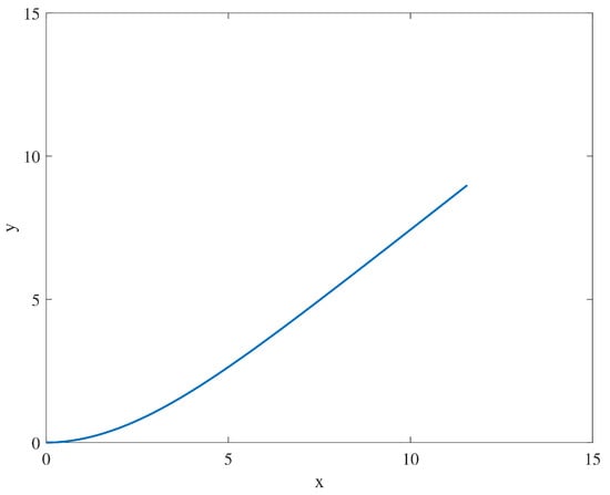
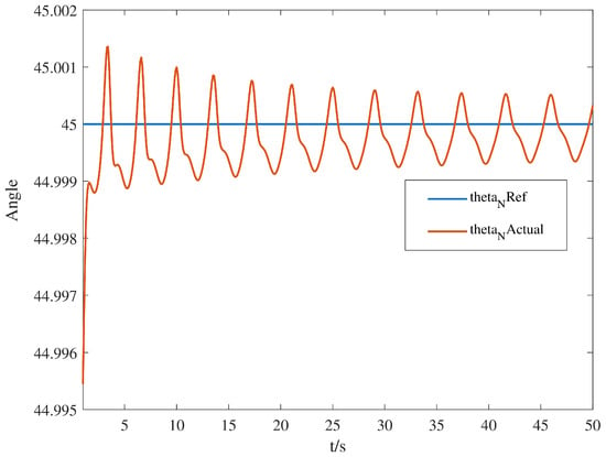
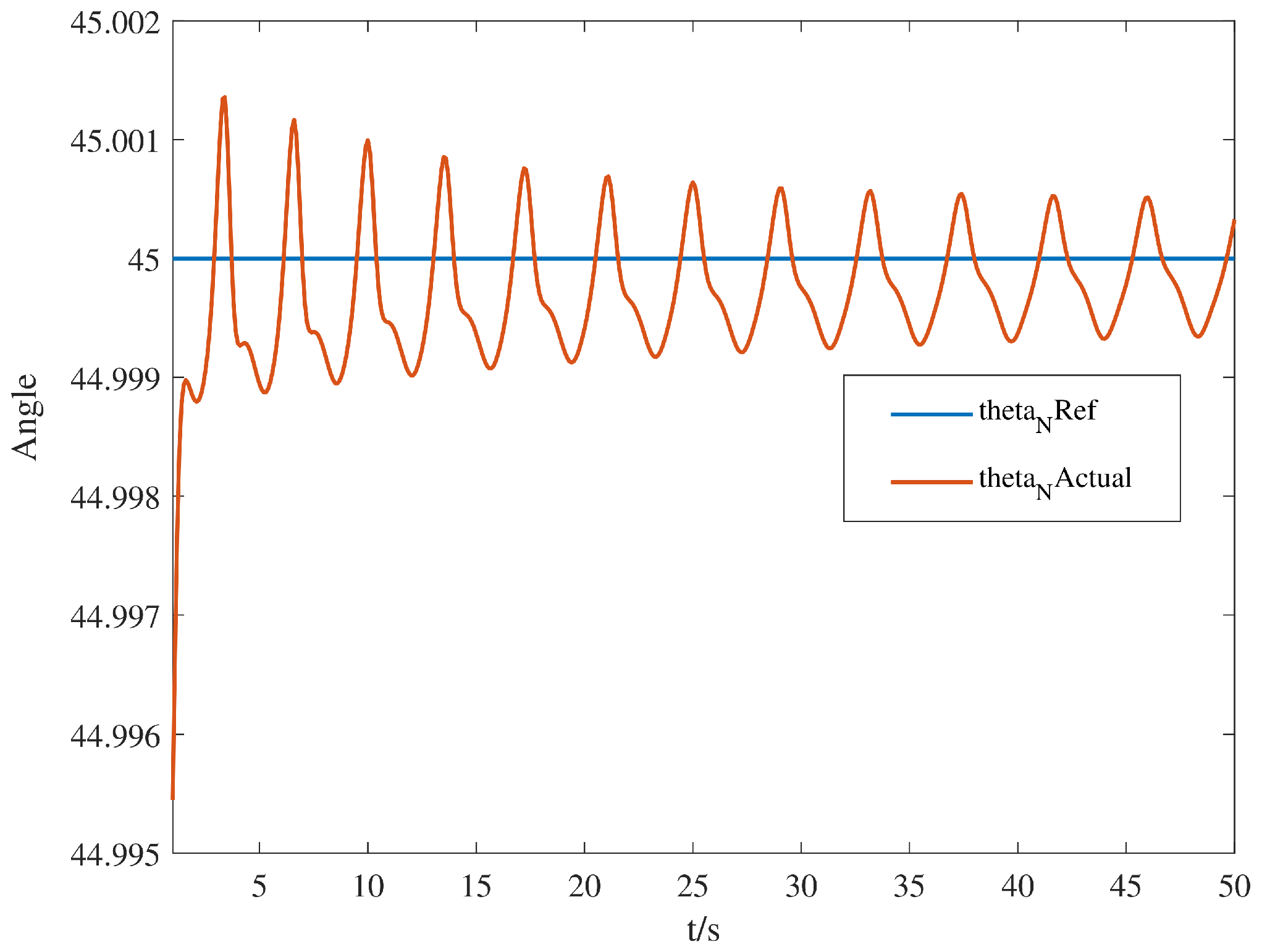
Figure 2 shows the simulated centroid trajectory, while Figure 3 compares the head-link heading to the ${45}^{\circ }$ reference. The centroid trajectory initially curves before transitioning to a straighter segment. Over the plotted interval, the head-link heading remains close to the reference, with small periodic deviations associated with the serpentine gait. Together, these results illustrate the robot’s directional response under the selected simulation conditions.

Figure 2. The centroid position of the snake robot.

Figure 3. The head angle of the snake robot.

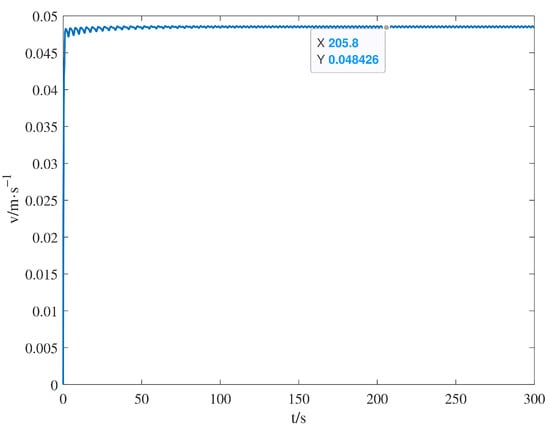
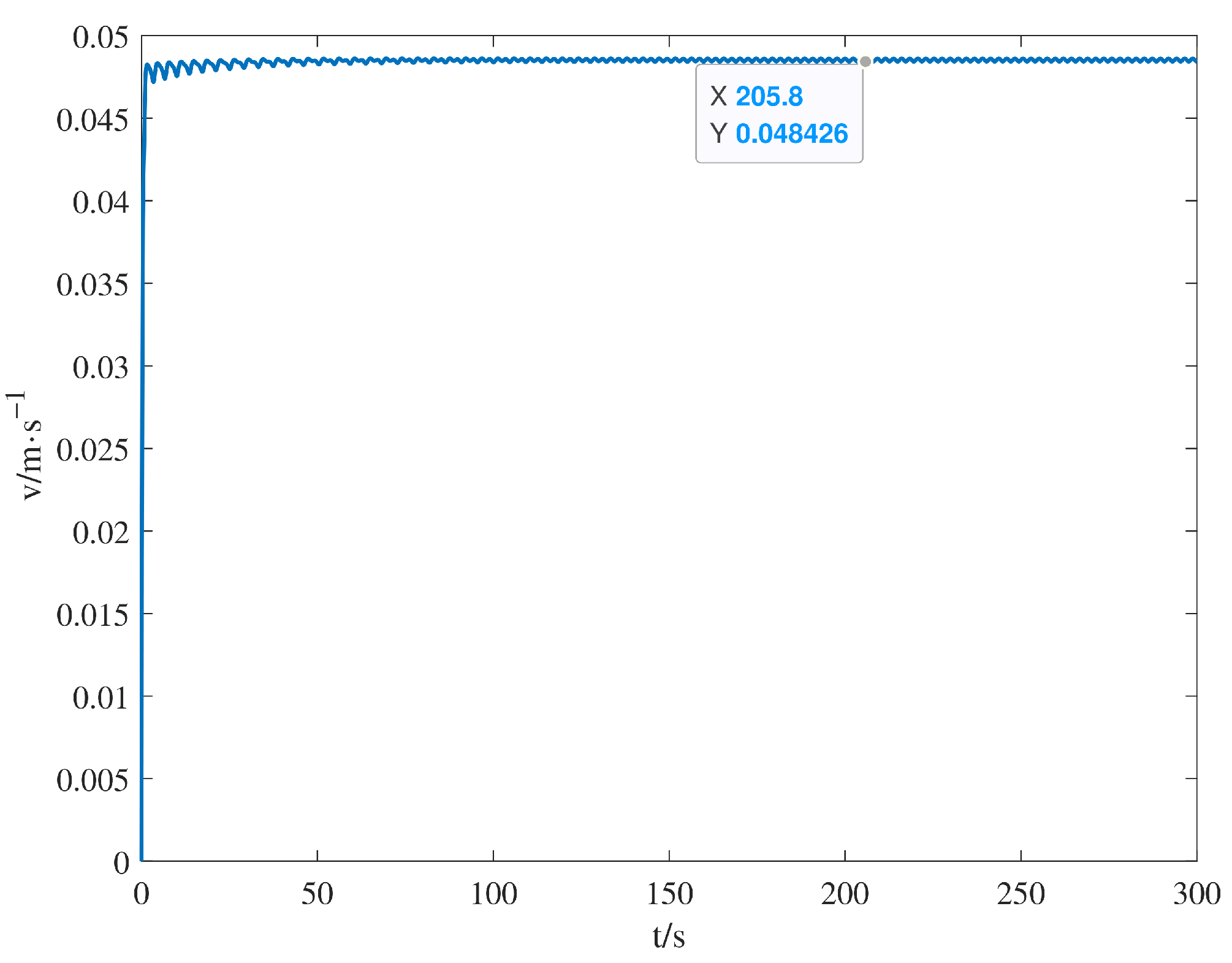
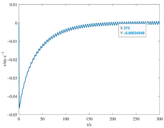
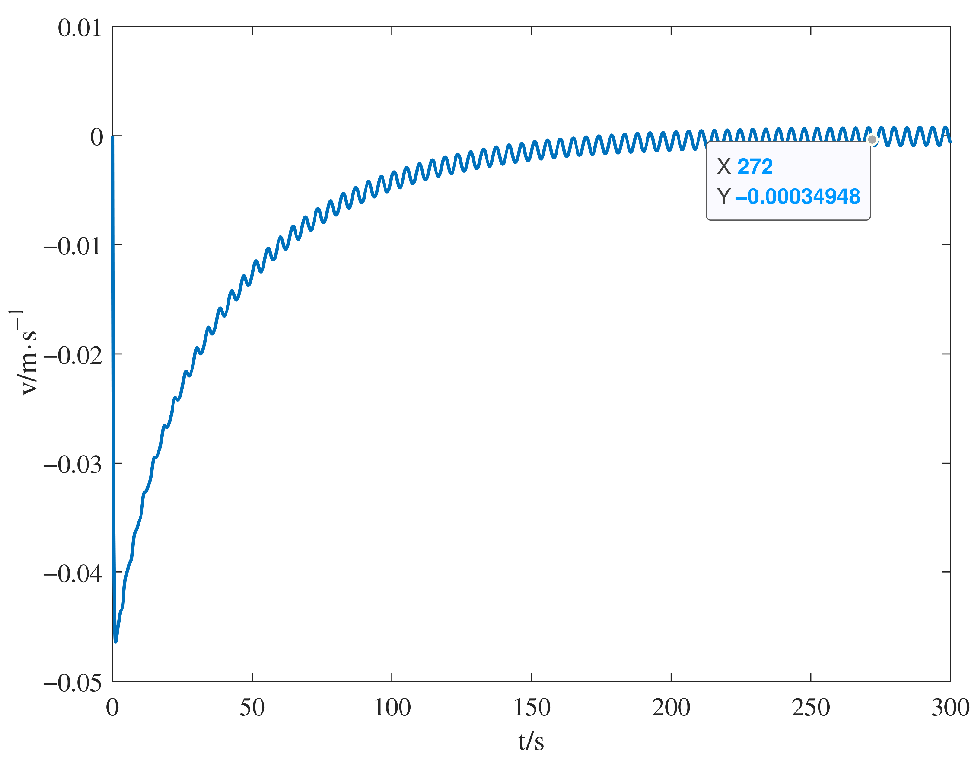
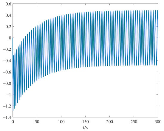
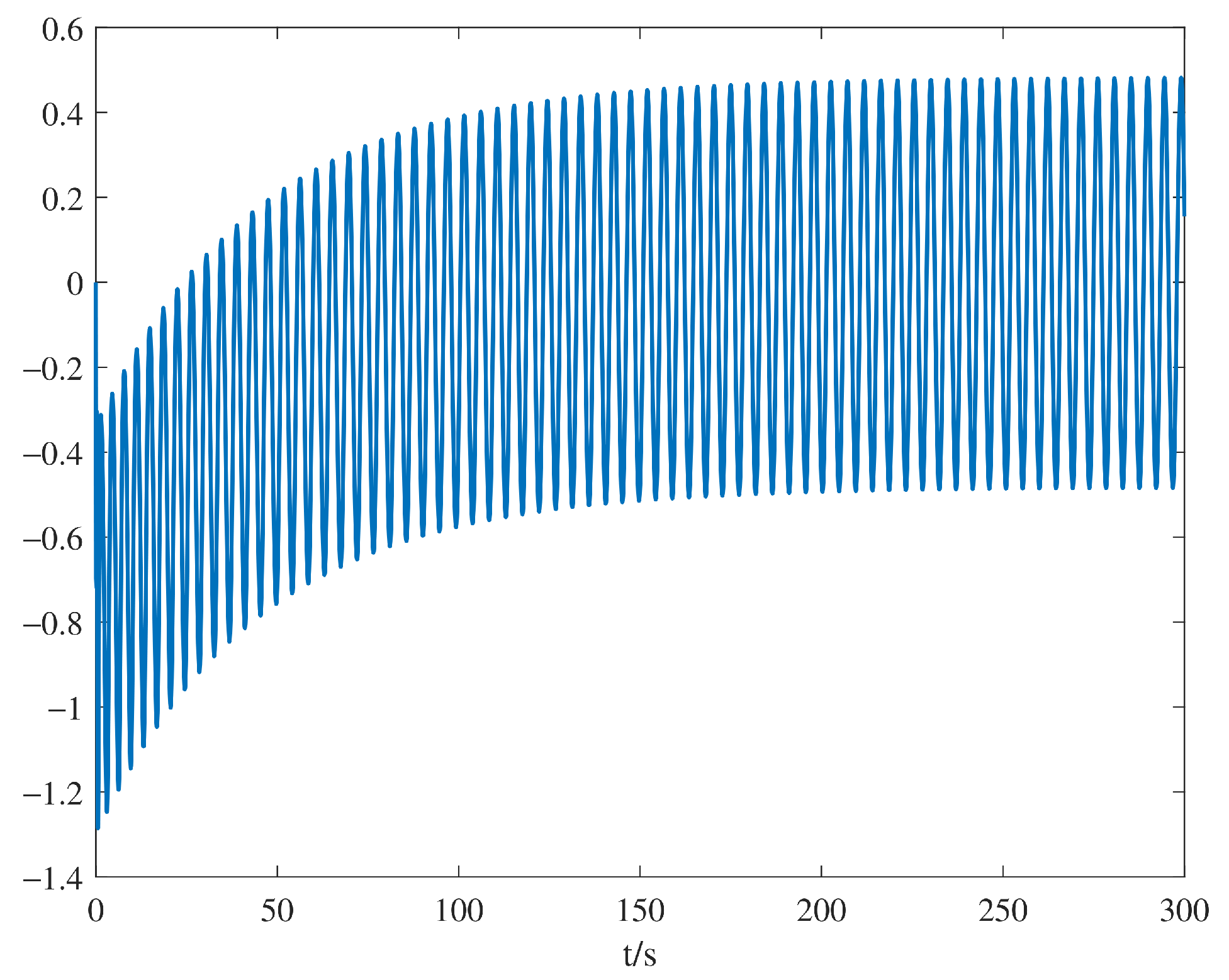
Figure 4 and Figure 5 show the tangential and normal components of the centroid velocity, respectively. In Figure 4, the tangential velocity settles into a nearly steady oscillatory response at approximately 0.048 m/s, remaining below the reference of 0.05 m/s. In Figure 5, the normal velocity approaches small oscillations around zero after the initial transient. These responses indicate predominantly forward locomotion with reduced lateral velocity in the illustrated simulation.

Figure 4. The tangential velocity of the snake robot.

Figure 5. The normal velocity of the snake robot.

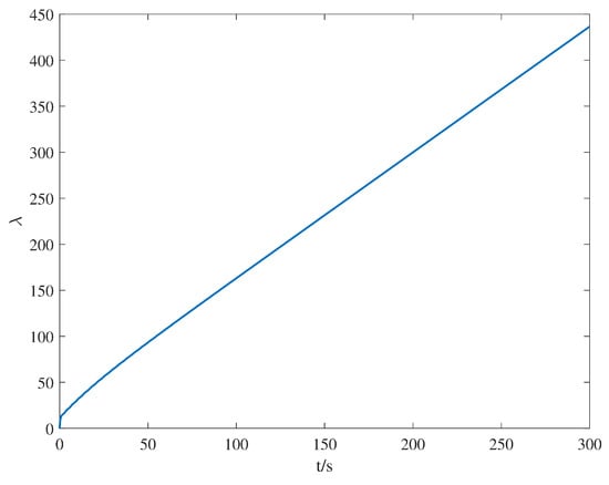
Figure 6 and Figure 7 show the steering offset ${\varphi }_0$ and the gait phase $\lambda$, respectively. After the initial adjustment, the steering offset exhibits bounded, periodic oscillations. The gait phase continues to increase and approaches a linear dependence on time, indicating an approximately constant phase rate during later motion. The steering offset ${\varphi }_0$ sets the reference angle for the joint adjacent to the head, whereas the advancing gait phase $\lambda$ governs the periodic evolution of the joint-angle references.

Figure 6. Time evolution of the steering offset ${\varphi }_0$.

Figure 7. Time evolution of the gait phase $\lambda$.

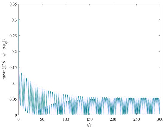
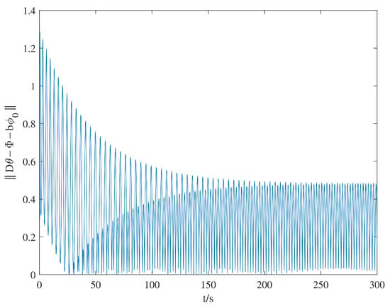
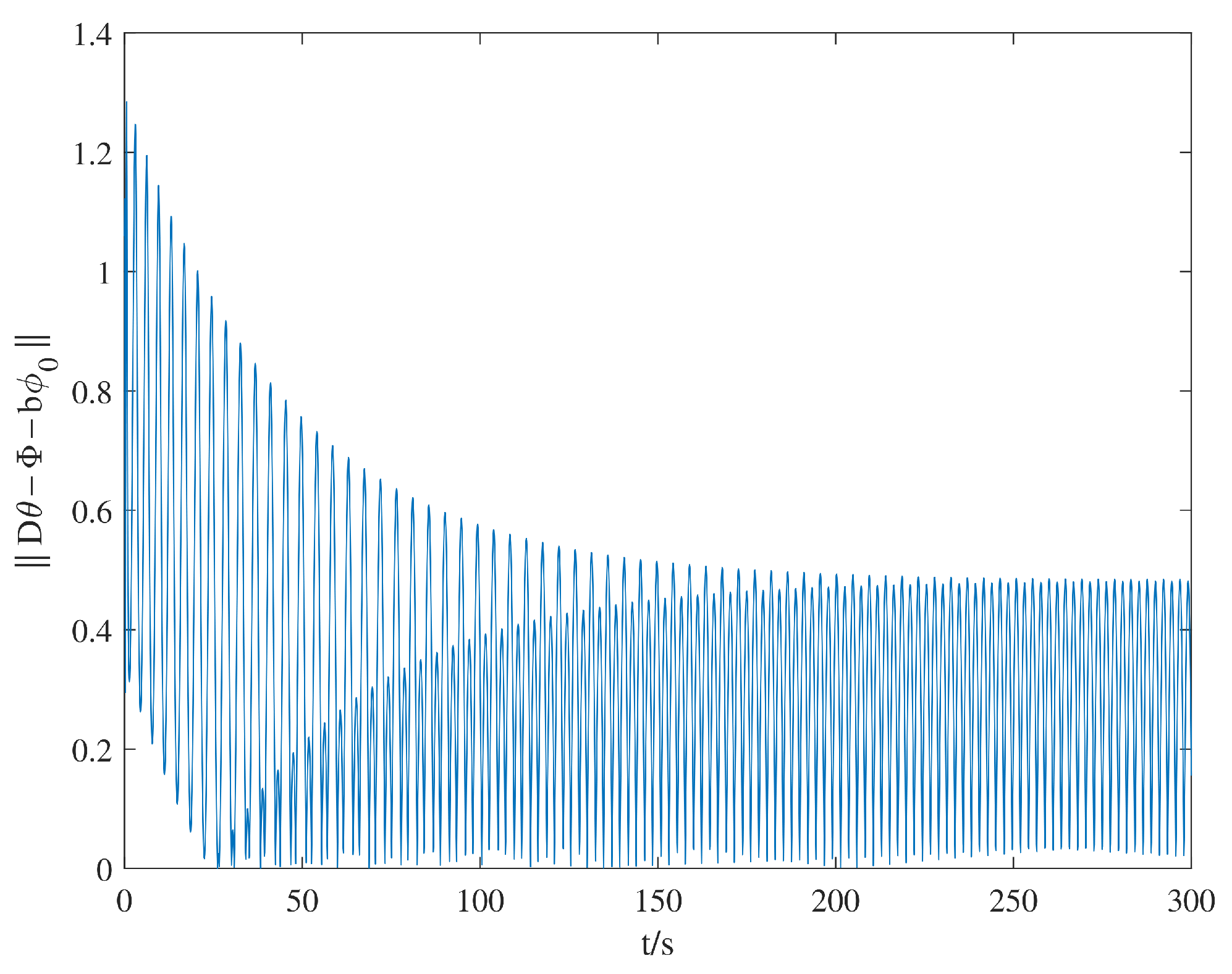
Figure 8 and Figure 9 assess joint tracking of the reference gait prescribed by the virtual holonomic constraints. Figure 8 shows the instantaneous mean absolute tracking error across joints, which quantifies the average deviation per joint. Figure 9 reports the Euclidean norm of the error vector, providing an aggregate measure of the discrepancy between the actual and reference joint configurations. Both measures exhibit oscillations with decreasing upper envelopes during the initial transient, followed by persistent periodic residuals. These responses indicate that the initial tracking mismatch is attenuated, although nonzero deviations from the prescribed gait persist during the subsequent motion.

Figure 8. Mean absolute joint tracking error.

Figure 9. Euclidean norm of the joint tracking error.

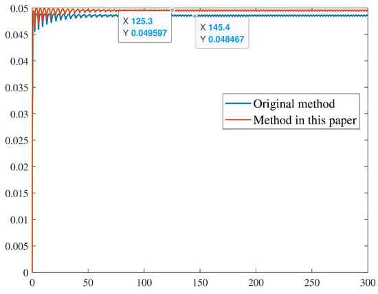
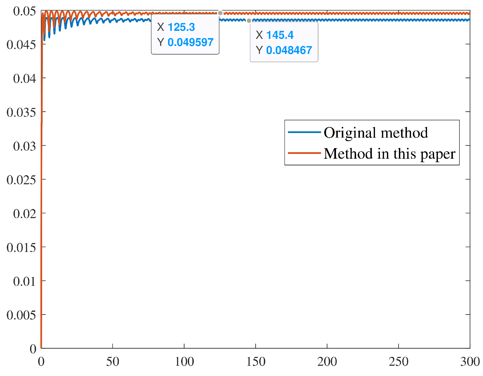
Figure 10 compares the tangential-velocity responses of the reference controller from Mohammadi et al. [43] and the controller proposed in this study. After the transient response, the proposed controller remains closer to the target speed of $0.05\mathrm{m}/\mathrm{s}$, though both responses exhibit small periodic oscillations. At this target speed, the reference controller converged to approximately $0.0485\mathrm{m}/\mathrm{s}$, whereas the proposed controller converged to approximately $0.0496\mathrm{m}/\mathrm{s}$. Accordingly, the proposed controller increased the converged tangential speed by approximately $0.0011\mathrm{m}/\mathrm{s}$ and reduced the absolute speed error relative to the target by approximately $73.3\%$.

Figure 10. Comparison of tangential-velocity tracking responses.

4.2. Physical Experiments

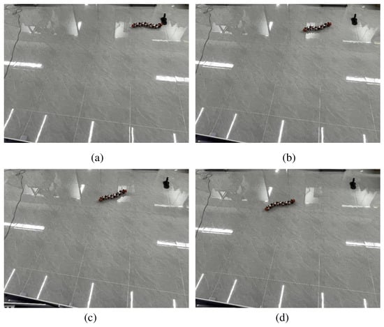
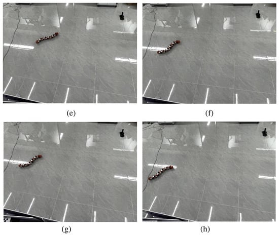
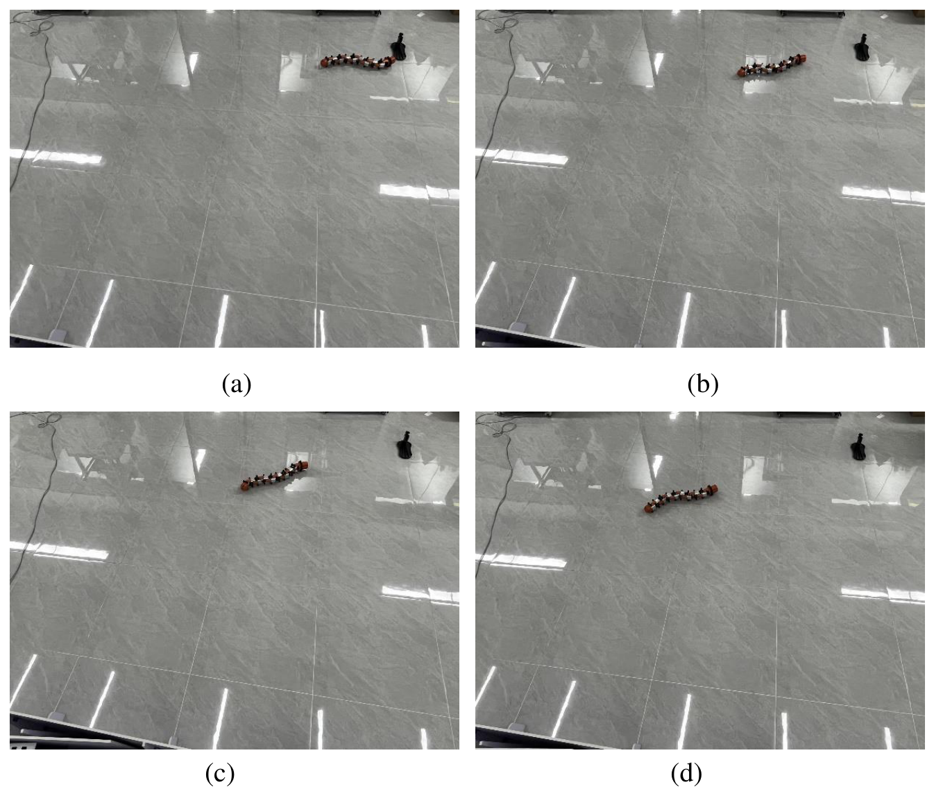
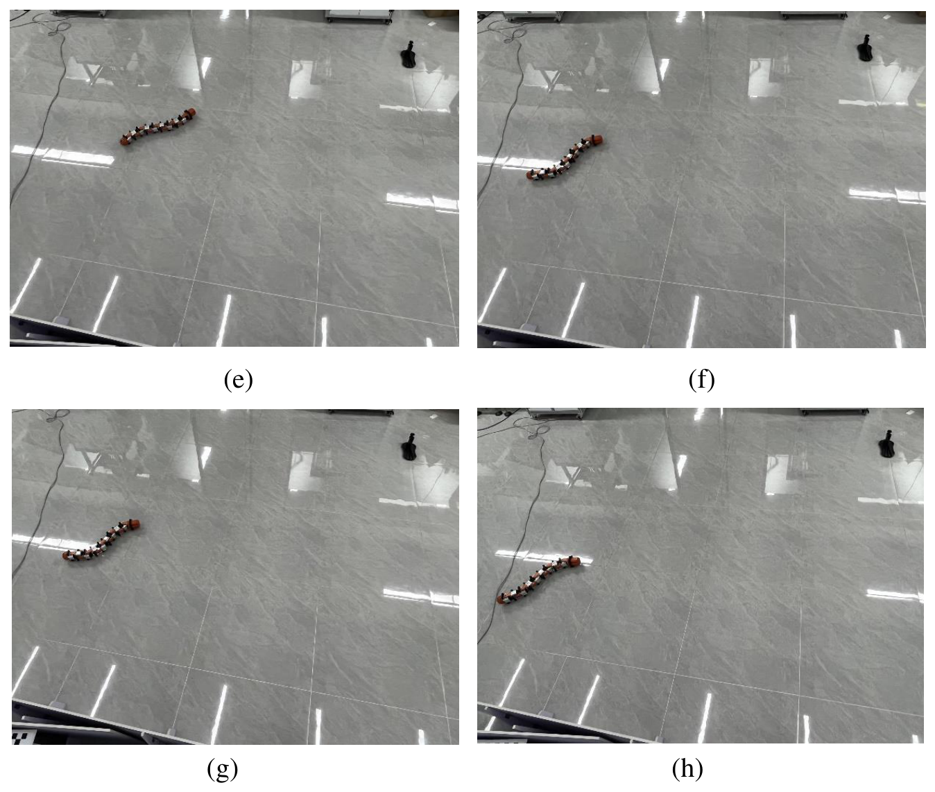
A physical experiment was conducted to examine the robot’s directional response under the implemented controller. Figure 11 presents successive snapshots of the robot during the experiment with a prescribed heading of ${\displaystyle \frac{\pi }{4}}\mathrm{rad}={45}^{\circ }$. Panels (a)–(d) show the early stage of motion, whereas panels (e)–(h) show subsequent changes in body configuration and orientation. The sequence provides qualitative evidence of heading adjustment on the physical platform under the tested conditions.

Figure 11. The results of the physical snake robot experiment. (a) Initial motion at a heading of $0^{\circ }$, with the body beginning to twist; (b) Start adjusting the direction, accompanied by a slight bend of the body; (c) The body orientation gradually approaches ${45}^{\circ }$; (d) Continuously twist the body towards the ${45}^{\circ }$ target direction; (e) The robot moves at ${45}^{\circ }$ with a small overall curvature; (f) The body distorts into a distinct S-shape to sustain movement; (g) The robot moves in an S-shaped towards ${45}^{\circ }$; (h) The robot successfully maintains a ${45}^{\circ }$ target orientation while moving.

The robot uses orthogonal joints, each driven by an ST3035 servo motor that accepts angle commands and provides joint-angle feedback. The head module houses the onboard computing board (Raspberry Pi), camera, IMU, illumination unit, and Wi-Fi communication module; the battery is housed in the tail. Servo commands and joint-angle measurements are exchanged over a TTL bus through a URT-1 serial-to-TTL converter.

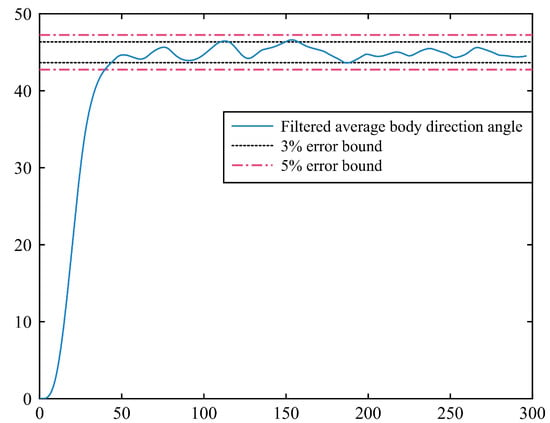
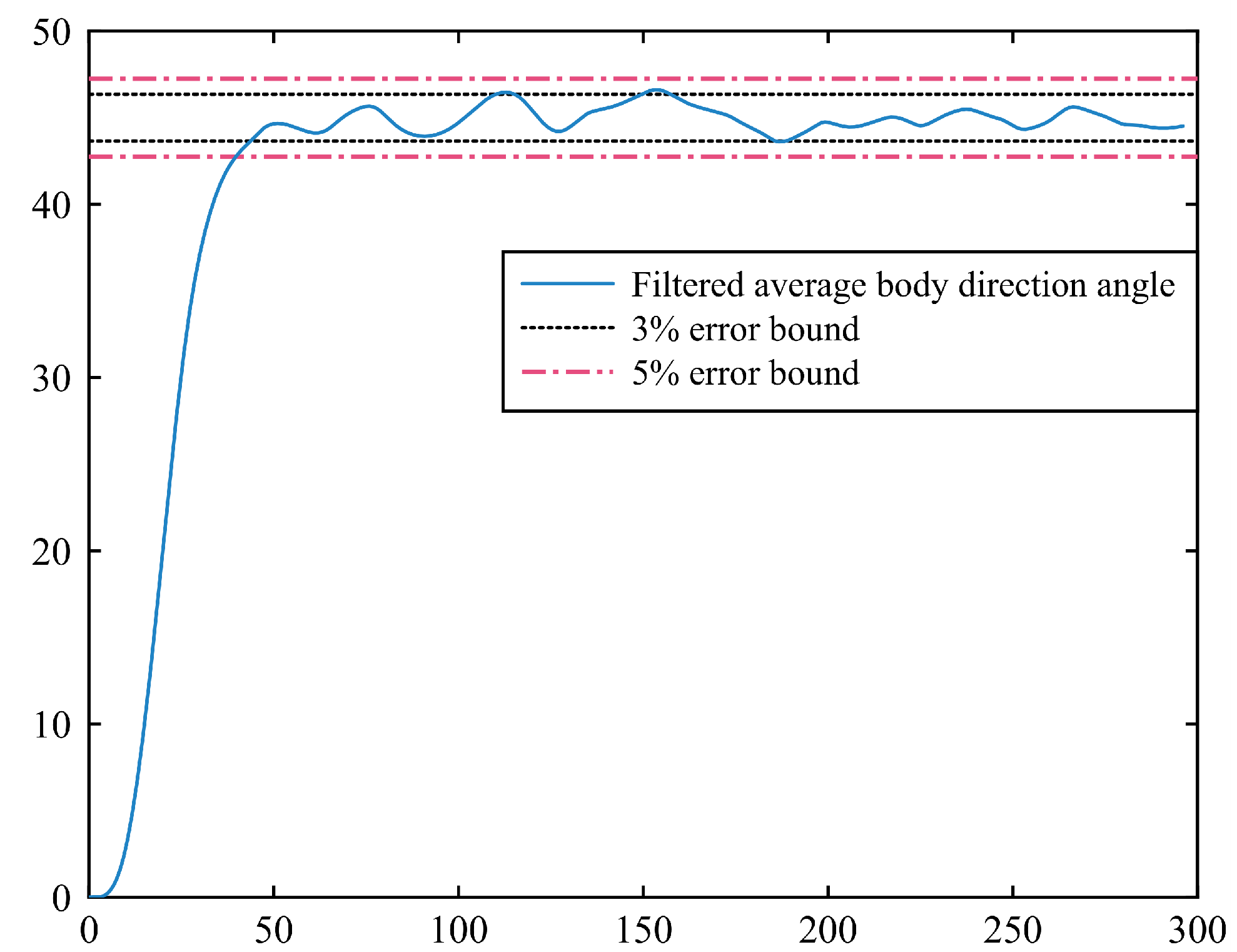
Figure 12 shows the heading response in the physical trial. The filtered average body-direction angle approaches the prescribed ${45}^{\circ }$ heading and remains within the $5\%$ error band after approximately $40\mathrm{s}$ and the $3\%$ band after approximately $190\mathrm{s}$. Meanwhile, this result reflects that each joint can track the desired joint angle well.

Figure 12. Average body-direction angle of the snake robot.

5. Discussion

The gait parameterization and reduced dynamics in Section 3 follow the VHC formulation of Mohammadi et al. [43], and the present study evaluates the implemented feedback design within this framework. The evaluated modification is the error-dependent term $g(v_e,\dot{\lambda })$ in the speed compensator. The numerical comparison shows improved speed regulation, reflected in a smaller final tangential-speed deviation, and the physical platform demonstrates heading adjustment. These results support the controller’s practical feasibility under the tested conditions. Further tests across reference speeds, friction conditions, and initial states, together with quantitative speed measurements on the physical platform, would help establish its performance over a broader operating range.

Figure 3 also shows small periodic deviations in the head-link orientation, which may be unfavorable for inspection cameras. Previous work has treated head orientation as a separate control objective through hierarchical VHC control [43] and head-trajectory tracking with actuator-failure robustness [50]. The present controller regulates locomotion heading rather than camera pose; stable head-pose tracking would require an additional control objective and dedicated validation and is left for future work.

6. Conclusions

In this paper, we first established the dynamic model of the snake robot based on geometric mechanics principles, obtaining the dynamical representation of the robot. Subsequently, we prescribed the snake robot’s serpentine gait through VHCs and derived the reduced nonlinear dynamics on the corresponding constraint manifold. Based on the VHC and backstepping methods, we devised controllers for the snake robot’s velocity direction and magnitude during its serpentine gait. Theoretical analysis demonstrates that the incorporation of new variables and velocity direction controllers enables the robot to converge to the desired direction of motion while maintaining Lyapunov stability. The simulation comparison showed an approximately 73.3% reduction in tangential-speed error. In the physical experiment, the heading error remained within the 5% and 3% tolerance bands after approximately $40\mathrm{s}$ and $190\mathrm{s}$, respectively. These results support the effectiveness of the proposed controller in speed and heading regulation.

References

- Zhang, H.; Li, L.; Jiang, A.; Xu, J.; Shen, H.; Li, Y.; Ji, A.; Wang, Z. LICFM3-SLAM: LiDAR-Inertial-Camera Fusion and Multimodal Multilevel Matching for Bionic Quadruped Inspection Robot Mapping. IEEE Trans. Instrum. Meas. 2025, 74, 1–17. [Google Scholar] [CrossRef] [Scilit]
- Sadasue, Y.; Nagae, H.; Takarabe, J.; Iwase, M. Development of Snake-Like Robot for Cable-Laying —Motion Design for Locomotion over Cable Racks and Ceiling Spaces. J. Robot. Mechatron. 2024, 36, 1408–1418. [Google Scholar] [CrossRef] [Scilit]
- Han, S.; Chon, S.; Kim, J.; Seo, J.; Shin, D.G.; Park, S.; Kim, J.T.; Kim, J.; Jin, M.; Cho, J. Snake Robot Gripper Module for Search and Rescue in Narrow Spaces. IEEE Robot. Autom. Lett. 2022, 7, 1667–1673. [Google Scholar] [CrossRef] [Scilit]
- Li, H.; Wang, G.; Li, L.; Wei, M.; Li, Y.; Sun, W.; Zeng, Q. Design of the swimming system of a bionic jellyfish robot for seabed exploration. Appl. Ocean Res. 2023, 134, 103498. [Google Scholar] [CrossRef] [Scilit]
- Zhang, Y.; Ge, Q.; Wang, Z.; Qin, Y.; Wu, Y.; Wang, M.; Shi, M.; Xue, L.; Guo, W.; Zhang, Y.; et al. Extracorporeal Closed-Loop Respiratory Regulation for Patients with Respiratory Difficulty Using a Soft Bionic Robot. IEEE Trans. Biomed. Eng. 2024, 71, 2923–2935. [Google Scholar] [CrossRef] [Scilit] [PubMed]
- Li, D.; Deng, H.; Pan, Z.; Xiu, Y. Collaborative obstacle avoidance algorithm of multiple bionic snake robots in fluid based on IB-LBM. ISA Trans. 2022, 122, 271–280. [Google Scholar] [CrossRef] [Scilit] [PubMed]
- Bellegarda, G.; Ijspeert, A. CPG-RL: Learning Central Pattern Generators for Quadruped Locomotion. IEEE Robot. Autom. Lett. 2022, 7, 12547–12554. [Google Scholar] [CrossRef] [Scilit]
- Sun, Y.; Pancheri, F.; Rehekampff, C.; Lueth, T.C. TurBot: A Turtle-Inspired Quadruped Robot Using Topology Optimized Soft-Rigid Hybrid Legs. IEEE/ASME Trans. Mechatron. 2024, 29, 3193–3202. [Google Scholar] [CrossRef] [Scilit]
- Ju, Z.; Wei, K.; Xu, Y. From Concept to Field Trials: Design, Analysis, and Evaluation of a Novel Quadruped Robot with Deformable Wheel–Foot Structure. IEEE Trans. Robot. 2025, 41, 3143–3161. [Google Scholar] [CrossRef] [Scilit]
- Fang, S.; Shi, S.; Wu, X.; Wang, X. A Walking and Climbing Quadruped Robot Capable of Ground-Wall Transition: Design, Mobility Analysis and Gait Planning. Intell. Serv. Robot. 2023, 16, 431–451. [Google Scholar] [CrossRef] [Scilit]
- Wang, Y.; Kamegawa, T.; Matsuda, E.; Gofuku, A. Motion Planning of a Snake Robot That Moves in Crowded Pipes. Adv. Robot. 2022, 36, 781–793. [Google Scholar] [CrossRef] [Scilit]
- Du, Z.; Fang, H.; Xu, J. Snake-worm: A Bi-modal Locomotion Robot. J. Bionic Eng. 2022, 19, 1272–1287. [Google Scholar] [CrossRef] [Scilit]
- Fukuoka, Y.; Otaka, K.; Takeuchi, R.; Shigemori, K.; Inoue, K. Mechanical Designs for Field Undulatory Locomotion by a Wheeled Snake-Like Robot with Decoupled Neural Oscillators. IEEE Trans. Robot. 2023, 39, 959–977. [Google Scholar] [CrossRef] [Scilit]
- Takemori, T.; Tanaka, M.; Matsuno, F. Adaptive Helical Rolling of a Snake Robot to a Straight Pipe with Irregular Cross-Sectional Shape. IEEE Trans. Robot. 2023, 39, 437–451. [Google Scholar] [CrossRef] [Scilit]
- Lu, J.; Tang, C.; Hu, E.; Li, Z. S-shaped rolling gait designed using curve transformations of a snake robot for climbing on a bifurcated pipe. Bioinspir. Biomim. 2024, 19, 036010. [Google Scholar] [CrossRef] [Scilit] [PubMed]
- Megalingam, R.K.; Senthil, A.P.; Raghavan, D.; Manoharan, S.K. Modeling of novel circular gait motion through daisy sequence fitting algorithm in a vertical climbing snake robot. J. Field Robot. 2024, 41, 211–226. [Google Scholar] [CrossRef] [Scilit]
- Huang, W.; Fang, Y.; Guo, X.; Liu, H.; Liu, L. A Unified Motion Modeling Approach for Snake Robot’s Gaits Generated with Backbone Curve Method. IEEE Trans. Robot. 2024, 40, 4132–4146. [Google Scholar] [CrossRef] [Scilit]
- Haghshenas-Jaryani, M. Dynamics and Computed-Muscle-Force Control of a Planar Muscle-Driven Snake Robot. Actuators 2022, 11, 194. [Google Scholar] [CrossRef] [Scilit]
- Wang, Y.; Tuo, G.; Li, T.; Shang, Z.; Lin, X.; Liu, X.; Liu, H. A Lie-Theory-Based Dynamics Modeling Method of Snake-Arm Robot with Virtual Linkage Criterion. J. Mech. Robot. 2025, 17, 111011. [Google Scholar] [CrossRef] [Scilit]
- Zhang, J.; Chen, Y.; Liu, Y.; Gong, Y. Dynamic Modeling of Underwater Snake Robot by Hybrid Rigid-Soft Actuation. J. Mar. Sci. Eng. 2022, 10, 1914. [Google Scholar] [CrossRef] [Scilit]
- Ahmed, S.; Gilbert, H.B. Kinestatic Modeling of a Spatial Screw-Driven Continuum Robot. IEEE Robot. Autom. Lett. 2022, 7, 3563–3570. [Google Scholar] [CrossRef] [Scilit]
- Zhang, J.; Chen, Y.; Gong, Y. Kinematics, dynamics, and control of underwater robotic snake based on a rigid-soft unified model. Ships Offshore Struct. 2024, 19, 1408–1423. [Google Scholar] [CrossRef] [Scilit]
- Ali, S. Dynamic modeling and simulation of a snake-like multibody robotic system with ground-adaptive strategy and efficient undulatory locomotion. Multibody Syst. Dyn. 2024, 62, 235–247. [Google Scholar] [CrossRef] [Scilit]
- Song, B.; Ju, I.; Yun, D. Optimizing snake robot locomotion with decomposed gait pattern representation. Integr. Comput.-Aided Eng. 2025, 32, 196–225. [Google Scholar] [CrossRef] [Scilit]
- Wang, W.; Gao, Z. A Variable Diameter Climbing Gait Design for a Snake Robot Based on the Bezier Curve. Int. J. Control. Autom. Syst. 2024, 22, 3753–3761. [Google Scholar] [CrossRef] [Scilit]
- Liu, X.; Lin, G.; Wei, W. Adaptive Transition Gait Planning of Snake Robot Based on Polynomial Interpolation Method. Actuators 2022, 11, 222. [Google Scholar] [CrossRef] [Scilit]
- Li, D.; Zhang, B.; Wu, C.; Xu, Y.; Huang, J.; Wu, E.Q.; Zhu, L. Tracking Control of Snake Robots with Butterfly Spiral Propulsion for Multiscenario Applications. IEEE Trans. Ind. Inform. 2024, 20, 13526–13536. [Google Scholar] [CrossRef] [Scilit]
- Zhang, J.; Ren, C.; Ma, S. Optimal Path Following Control for Motion Recovery from Joint Failure of Snake Robots Using Improved Lateral Undulatory Gait. IEEE/ASME Trans. Mechatron. 2025, 30, 3161–3169. [Google Scholar] [CrossRef] [Scilit]
- Sheng, F.; Wan, F.; Tang, C.; Guo, X. A Maneuverable Winding Gait for Snake Robots Based on a Delay-Aware Swing and Grasp Framework Combining Rules and Learning Methods. IEEE Robot. Autom. Lett. 2025, 10, 311–318. [Google Scholar] [CrossRef] [Scilit]
- Zhao, W.; Wang, J.; Fei, Y. A Multigait Continuous Flexible Snake Robot for Locomotion in Complex Terrain. IEEE/ASME Trans. Mechatron. 2022, 27, 3751–3761. [Google Scholar] [CrossRef] [Scilit]
- Tang, C.; Sun, L.; Zhou, G.; Shu, X.; Tang, H.; Wu, H. Gait Generation Method of Snake Robot Based on Main Characteristic Curve Fitting. Biomimetics 2023, 8, 105. [Google Scholar] [CrossRef] [Scilit] [PubMed]
- Elsayed, B.A.; Takemori, T.; Tanaka, M.; Matsuno, F. Mobile Manipulation Using a Snake Robot in a Helical Gait. IEEE/ASME Trans. Mechatron. 2022, 27, 2600–2611. [Google Scholar] [CrossRef] [Scilit]
- Yang, Z.; Fang, Z.; Yang, S.; Xiong, Y.; Zhang, D. Research on the Spiral Rolling Gait of High-Voltage Power Line Serpentine Robots Based on Improved Hopf-CPGs Model. Appl. Sci. 2025, 15, 1285. [Google Scholar] [CrossRef] [Scilit]
- Simoes, A.A.; Stratoglou, E.; Bloch, A.; Colombo, L.J. Virtual nonholonomic constraints: A geometric approach. Automatica 2023, 155, 111166. [Google Scholar] [CrossRef] [Scilit]
- Patel, B.M.; Dwivedy, S.K. Virtual holonomic constraints based super twisting sliding mode control for motion control of planar snake robot in the uncertain underwater environment. Proc. Inst. Mech. Eng. Part I J. Syst. Control Eng. 2023, 237, 1480–1491. [Google Scholar] [CrossRef] [Scilit]
- Kakaei, M.M.; Salarieh, H.; Sohrabpour, S. Online regulation of walking gait speed for a five-link bipedal robot via adaptive deforming of virtual holonomic constraints. Nonlinear Dyn. 2023, 111, 20055–20071. [Google Scholar] [CrossRef] [Scilit]
- Li, X.; Ren, C.; Ma, S. Optimal Path Following Control with Efficient Computation for Snake Robots Subject to Multiple Constraints and Unknown Frictions. IEEE Robot. Autom. Lett. 2022, 7, 9151–9158. [Google Scholar] [CrossRef] [Scilit]
- Li, D.; Zeng, L.; Xiu, Y.; Pan, Z.; Zhang, D.; Deng, H. Sideslip Elimination and Coefficient Approximation-Based Trajectory Tracking Control for Snake Robots. IEEE Trans. Ind. Inform. 2023, 19, 8754–8764. [Google Scholar] [CrossRef] [Scilit]
- Liu, Z.; Wei, W.; Liu, X.; Han, S. Target Tracking of Snake Robot with Double-Sine Serpentine Gait Based on Adaptive Sliding Mode Control. Actuators 2023, 12, 38. [Google Scholar] [CrossRef] [Scilit]
- Li, D.; Zhang, B.; Li, P.; Wu, E.Q.; Law, R.; Xu, X.; Song, A.; Zhu, L.M. Parameter Estimation and Anti-Sideslip Line-of-Sight Method-Based Adaptive Path-Following Controller for a Multijoint Snake Robot. IEEE Trans. Syst. Man Cybern. Syst. 2023, 53, 4776–4788. [Google Scholar] [CrossRef] [Scilit]
- Xiu, Y.; Li, D.; Zhang, M.; Deng, H.; Law, R.; Huang, Y.; Wu, E.Q.; Xu, X. Finite-Time Sideslip Differentiator-Based LOS Guidance for Robust Path Following of Snake Robots. IEEE/CAA J. Autom. Sin. 2023, 10, 239–253. [Google Scholar] [CrossRef] [Scilit]
- Li, D.; Wu, C.; Liu, G.; Zhu, L.; Wu, E.Q. Synchronous Obstacle Avoidance Tracking Control Scheme for Snake Robots with State Constraints and Interference Compensation. IEEE Trans. Ind. Electron. 2026, 73, 873–884. [Google Scholar] [CrossRef] [Scilit]
- Mohammadi, A.; Rezapour, E.; Maggiore, M.; Pettersen, K.Y. Maneuvering Control of Planar Snake Robots Using Virtual Holonomic Constraints. IEEE Trans. Control Syst. Technol. 2016, 24, 884–899. [Google Scholar] [CrossRef] [Scilit]
- Reyhanoglu, M.; van der Schaft, A.; McClamroch, N.H.; Kolmanovsky, I. Dynamics and control of a class of underactuated mechanical systems. IEEE Trans. Autom. Control 1999, 44, 1663–1671. [Google Scholar] [CrossRef] [Scilit]
- Khalil, H.K. Nonlinear Systems, 3rd ed.; Prentice Hall: Hoboken, NJ, USA, 2002. [Google Scholar]
- Maggiore, M.; Consolini, L. Virtual Holonomic Constraints for Euler–Lagrange Systems. IEEE Trans. Autom. Control 2013, 58, 1001–1008. [Google Scholar] [CrossRef] [Scilit]
- Blekhman, I.I. Vibrational Mechanics: Nonlinear Dynamic Effects, General Approach, Applications; World Scientific: Singapore, 2000. [Google Scholar]
- Arnold, V.I.; Kozlov, V.V.; Neishtadt, A.I. Mathematical Aspects of Classical and Celestial Mechanics, 3rd ed.; Springer: Berlin/Heidelberg, Germany, 2006. [Google Scholar]
- Kokotovic, P.V.; Khalil, H.K.; O’Reilly, J. Singular Perturbation Methods in Control: Analysis and Design; SIAM: Philadelphia, PA, USA, 1999. [Google Scholar]
- Ariizumi, R.; Takahashi, R.; Tanaka, M.; Asai, T. Head-trajectory-tracking control of a snake robot and its robustness under actuator failure. IEEE Trans. Control Syst. Technol. 2019, 27, 2589–2597. [Google Scholar] [CrossRef] [Scilit]
Disclaimer/Publisher’s Note: The statements, opinions and data contained in all publications are solely those of the individual author(s) and contributor(s) and not of MDPI and/or the editor(s). MDPI and/or the editor(s) disclaim responsibility for any injury to people or property resulting from any ideas, methods, instructions or products referred to in the content. |
© 2026 by the authors. Licensee MDPI, Basel, Switzerland. This article is an open access article distributed under the terms and conditions of the Creative Commons Attribution (CC BY) license.