


Abstract
This work presents a sampling-based Quadratic Stability Control (QSC) framework for nonlinear mechanical systems with parametric uncertainty and compares it with a nominal Linear Quadratic Regulator (LQR). The proposed method synthesizes a single state-feedback gain by enforcing a common quadratic Lyapunov condition over a finite set of locally linearized models sampled in state and parameter space. A systematic numerical study evaluates the effects of the number of sampled models, state sampling radius, parameter uncertainty, and actuator configuration. Performance is assessed using trajectory mean-squared error, final position error, and offline controller-synthesis time. The results show that QSC has higher position error than nominal LQR at 5% uncertainty but lower error at 10% and 15% across five independently sampled designs, with greater force effort while maintaining comparable nominal performance. The common quadratic certificate covers the sampled models and their convex hull, not the full continuous nonlinear domain. These benefits are obtained at the cost of higher offline semidefinite-programming complexity.
1. Introduction
This paper considers the regulation of a planar elastic lattice composed of masses connected to their neighbors and rigid boundaries by axial and diagonal springs and dampers. Planar forces applied to selected masses must maintain a desired, dynamically feasible configuration despite uncertainty in the masses, stiffnesses, damping coefficients and grid spacing. The control-design problem is to obtain one constant state-feedback gain that satisfies a common quadratic Lyapunov condition for local models representing both state deviations and physical-parameter variation.
Although the springs are linear in elongation, their force directions change with the lattice geometry, making the coupled dynamics nonlinear. Consequently, the local Jacobians vary as the masses move away from the reference configuration and as the physical parameters depart from their nominal values. A controller synthesized at one nominal linearization therefore does not establish stability for the other local models or bound the resulting regulation error. Parameter changes can also shift the equilibrium associated with the reference input, leaving a nonzero drift at the nominal reference; a common certificate for homogeneous linearized dynamics alone does not remove this offset.
We address this problem using sampling-based Quadratic Stability Control (QSC). Offline, states are sampled from a ball around a feasible reference operating point, while physical parameters are sampled from a relative componentwise box around their nominal values. Each sampled state–parameter pair defines a local state and input Jacobian, and the nominal model is included in the synthesis family. A semidefinite feasibility problem then finds one feedback gain and one common quadratic Lyapunov matrix for all these local models, using a standard change of variables to obtain linear matrix inequalities (LMIs). This directly includes changes in both the linearization location and the physical parameters without constructing an explicit enclosure of the continuous Jacobian family. The certificate applies to the homogeneous sampled closed-loop matrices and their matrix convex hull; it does not establish stability throughout the continuous nonlinear state–parameter domain. The implemented controller uses full-state feedback, with no online parameter estimation or gain scheduling. We evaluate its regulation performance on the original nonlinear lattice against nominal unit-weight Linear Quadratic Regulator (LQR), varying sample count, state-sampling radius, parameter uncertainty and actuator configuration.
Lyapunov-based methods are widely used in the analysis and control of nonlinear systems [1,2]. The requirement that one Lyapunov function decrease for several local models connects QSC to common Lyapunov analysis of nonlinear families. Branicky’s work on switched nonlinear systems shows why stability of individual subsystems does not by itself ensure stability when the active dynamics change [1]. For the lattice considered here, the dynamics vary smoothly with geometry, and the physical parameters are uncertain rather than switched by a prescribed law. Constructive results for nonlinear families require suitable structural assumptions: Vu and Liberzon construct local and global common Lyapunov functions for finite families of pairwise commuting globally asymptotically stable nonlinear systems [3]. Applying this principle to the nonlinear plant would require a condition throughout a shared state–parameter domain; QSC imposes it on the homogeneous dynamics of finitely many local linearizations.
The mechanical structure makes the choice of a common function particularly important. Kinetic and elastic potential energy are natural Lyapunov candidates for a fixed passive spring system [4], but their dependence on masses and stiffnesses means that they do not automatically provide a parameter-independent certificate for the controlled lattice. Aleksandrov et al. explicitly construct common Lyapunov functions for families of mechanical systems with switching linear force fields [5]. For classes of nonlinear mechanical systems with one degree of freedom, Aleksandrov and Murzinov obtain common Lyapunov conditions [6]. Their analysis establishes the relevance of common functions to mechanical families, although its conditions do not directly provide a feedback design for the coupled planar lattice studied here. This motivates the use of a quadratic function that can be sought jointly with a controller for the lattice’s local models.
For a family of linear models, this joint search can be expressed through common quadratic Lyapunov inequalities and a change of synthesis variables [7]. Requiring one Lyapunov matrix keeps the sampled synthesis tractable, but can exclude families that admit more general certificates, as discussed in the review by Shorten et al. [8]. Oliveira and Peres address this restriction through affine parameter-dependent Lyapunov functions for matrix polytopes [9]; Pipeleers et al. develop extended LMI characterizations for stability and performance [10]. In the present problem, the family must also represent changes in the linearization location. Shamma and Athans analyze conditions under which local gain-scheduled designs yield stability and robustness properties for nonlinear plants [11]. Leith and Leithead’s gain-scheduling survey discusses the relationship between nonlinear dynamics and families of local linear models [12]. Within that setting, Shimomura and Kubotani revisit conservatism under common Lyapunov functions and demonstrate their design on a mass–damper–spring system [13]. QSC retains a single gain while incorporating nearby linearization locations into the synthesis family. These locations represent state deviations around the reference; their inclusion does not certify regulation about every equilibrium shifted by parameter uncertainty.
Representing both sources of variation leads to sampling in the joint state–parameter space. Sampling only parameters at the reference would omit changes in the Jacobians caused by lattice motion, whereas sampling only states at nominal parameters would omit physical-model mismatch. Calafiore and Campi’s scenario approach provides a related framework for enforcing uncertain control-design constraints at sampled realizations [14]. Campi et al. explain the algorithmic use of sampled constraints for systems and control design [15], while Campi and Garatti establish probabilistic feasibility results for uncertain convex programs under the assumptions of their scenario formulation [16]. Here, joint samples are used to construct a finite common-gain feasibility problem, and no prescribed probabilistic violation bound is claimed. The resulting controller is assessed separately on nonlinear trajectories, allowing the numerical study to examine how sampling choices and parameter uncertainty affect regulation beyond the certified linear models.
The contributions of this paper are:
- a constant-gain synthesis procedure imposing one common quadratic Lyapunov condition on Jacobians sampled jointly in state and parameter space;
- nonlinear evaluations of sample count, state radius, parameter uncertainty and actuator placement, using position-only error metrics;
- comparisons over five independently synthesized QSC gains that quantify performance at three parameter-uncertainty levels;
- sampling-law experiments and measurements of offline synthesis cost as the lattice dimension grows.
2. Preliminaries
Table 1 summarizes the main notation used throughout the paper.
Table 1.
Summary of main notation.
Consider the nonlinear dynamical system
where denotes the system state, is the control input, and represents a vector of uncertain but bounded physical parameters. The function is assumed to be twice continuously differentiable with respect to the state and input in the region considered.
Let denote a nominal point of interest. In the present problem, this point need not be an exact equilibrium for every admissible parameter value. The control objective is therefore formulated in terms of the local feedback dynamics around this point and subsequently evaluated on the original nonlinear system.
2.1. Local Linearization
For a fixed parameter vector , define the state and input deviations by and . A first-order Taylor expansion of (1) around gives
where
and
is the local drift term.
At an exact equilibrium, . The reference-generation procedure in Section 5 gives a numerically settled nominal operating point; it does not make that point an equilibrium for every uncertain parameter value. The LMIs below concern homogeneous Jacobian dynamics. The affine residual and nonlinear terms remain in the simulations.
2.2. Quadratic Stability
Quadratic stability is based on the existence of a common quadratic Lyapunov function. Consider the linear time-invariant system
The system is quadratically stable if there exists a symmetric positive-definite matrix such that
and
which is equivalent to
For the locally linearized input system, consider the state-feedback law
where is constant. The corresponding homogeneous closed-loop dynamics are
The closed-loop system is quadratically stable if there exists satisfying
Condition (11) is bilinear in P and K. Introducing
and applying a congruence transformation yields the LMI
which is affine in the decision variables X and Y. If a feasible solution is obtained, the feedback gain is recovered as
3. Problem Formulation
This section formalizes the control objective and distinguishes the finite-sample stability certificate from the subsequent nonlinear simulation-based evaluation. The objective is to construct one state-feedback gain that stabilizes the feedback dynamics of a finite family of local linearizations generated over a prescribed neighborhood of the operating point and a bounded parameter set.
Problem Statement
Problem 1.
Given the nonlinear system (1), a nominal point of interest , and the sampling set
determine a constant state-feedback gain K and a symmetric matrix such that
for the N sampled linearized models generated from points .
The resulting condition is a finite-sample quadratic stability certificate: it guarantees a common quadratic Lyapunov function for the sampled linear models used in synthesis. It does not, by itself, constitute a formal stability proof for every point in the continuous nonlinear state–parameter region. The latter is investigated numerically through independent closed-loop simulations.
Remark 1.
Each sampled model contributes one LMI constraint, so the number of LMI constraints grows linearly with the number of samples N. This does not imply that the numerical solution time scales linearly with N, since the cost of solving the resulting semidefinite program also depends on the decision-variable dimensions, solver implementation, and numerical conditioning. Increasing the sampling radius or the number of samples can improve coverage of the region of interest, but may also increase conservatism or computational cost. The controller design therefore involves a trade-off between coverage, robustness, and offline synthesis time.
4. Proposed Method
This section presents the proposed sampling-based Quadratic Stability Control (QSC) procedure. The method consists of two stages. First, local linearizations are sampled over a prescribed neighborhood in state and parameter space. Second, a single state-feedback gain is synthesized by imposing a common quadratic Lyapunov condition on all sampled models.
4.1. Sampling in a Neighborhood of the Operating Point
Let the state neighborhood be the closed ball
where specifies the range of state deviations considered during synthesis. Similarly, parameter uncertainty is represented by
where is the relative half-width of the componentwise parameter box used in the experiments. The combined sampling region is
A finite collection of state–parameter pairs is drawn according to the sampling procedure used in the numerical study,
where denotes the uniform distribution over the specified product set. The sampled points provide a finite approximation of the variation of the local Jacobian over the region of interest.
For each sampled pair, the nonlinear system is linearized at , with the reference input held fixed. The resulting Jacobian matrices are
The associated linearized feedback dynamics are represented as
where denotes a perturbation about the sampled linearization point. The constant drift of the nonlinear model at an individual sampled point is not included in the homogeneous LMI condition; it is retained when the resulting controller is evaluated on the original nonlinear dynamics.
4.2. Controller Synthesis
The proposed controller is a single constant state-feedback gain K shared by all sampled models. For each , quadratic stability is imposed through
Thus, the same matrix P is used for every sampled model, providing a common quadratic Lyapunov function for the finite sampled family.
The synthesis problem is therefore a semidefinite feasibility problem with N sampled stability constraints. The implementation additionally includes the nominal model, giving stability blocks. Once a feasible solution is found, the controller gain is recovered using Equation (14).
The finite set of LMIs certifies quadratic stability only for the sampled linearized models. Increasing N provides a denser representation of the prescribed region but does not, by itself, establish a continuous-region certificate. The numerical experiments therefore assess the resulting controller on independently generated nonlinear trajectories and perturbed parameter realizations.
The state sampling radius r controls the extent of the region represented during synthesis. A larger radius exposes the controller to stronger variations in the nonlinear Jacobian, but, for a fixed number of samples, also reduces the sampling density within the region. Consequently, r and N jointly determine the coverage and conservatism of the sampled controller design.
4.3. Certificate Scope and Design Choices
The common quadratic function certifies the homogeneous sampled closed-loop matrices and their convex hull. It does not guarantee stability for all unsampled state–parameter pairs, nonlinear trajectories or clipped inputs. Because the reference operating point need not be an exact equilibrium under perturbed parameters, the drift term is generally nonzero and the local dynamics take the form . For the local affine approximation, if is Hurwitz, the constant residual gives an equilibrium error . The sampled homogeneous LMI does not establish boundedness of nonlinear trajectories under this drift. The lattice is control affine with a state-independent force Jacobian for each fixed parameter vector.
In practice, the parameter-box half-width should be chosen from physically justified identification or manufacturing bounds, and the state domain from expected deviations and admissible geometry. The state ball uses the benchmark numerical coordinates, which include positions and velocities; r is not a displacement in metres. The number of samples trades computation against the representation of local Jacobian variation. Section 5.6.1 reports its observed effect on controller performance; independently redrawn sample families need not exhibit monotone error trends.
Uniform-volume sampling uses a normalized Gaussian direction and radius , , with independent uniform parameter components. A centre-biased law would emphasize nominal behaviour while potentially missing boundary constraints; a boundary-enriched law could expose difficult models and restrict feasibility. Appendix A compares these radial laws on common test cases.
5. Numerical Model and Results
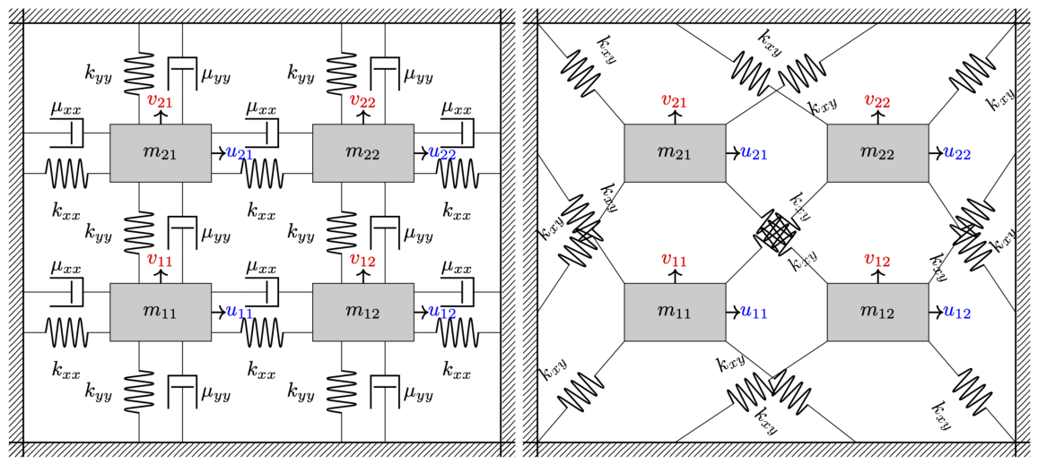
We consider an lattice of identical point masses, each of mass m, arranged in a planar grid and surrounded by rigid walls. Each mass is connected to its nearest neighbors and to the surrounding boundaries via linear springs and viscous dampers. The interconnections include both axial and diagonal elements, resulting in nonlinear coupling due to geometric effects. Here and count grid rows and columns; l and k below denote grid spacing and axial spring stiffness.
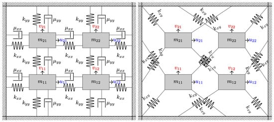
Figure 1 depicts the mass–spring–damper lattice model. The interconnections are split across two subfigures solely for visualization purposes, in order to clearly illustrate the axial and diagonal spring–damper couplings without altering the underlying system structure. In the schematic, and denote the common horizontal and vertical stiffness and damping; denotes diagonal stiffness. Diagonal damping is included in the model but is not drawn in the schematic. The and c in Equation (23) are generic coefficients of one connection: for axial connections and for diagonal connections. The spring rest length in the model is for axial connections and for diagonal connections, where l is the grid spacing parameter.
Figure 1.
Mass–spring–damper lattice model. Axial springs and dampers and diagonal springs are shown; diagonal damping is included in the model but omitted from the schematic.
5.1. Equations of Motion
The dynamics of each mass are derived using Newton’s second law. Let
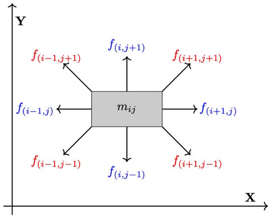
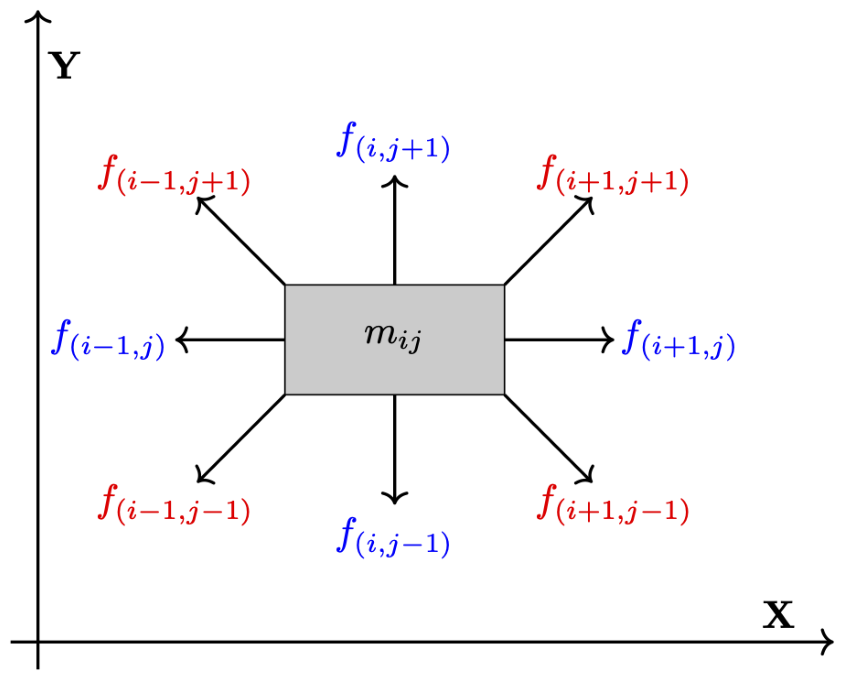
denote the planar position of the mass located at grid position , with and . Figure 2 illustrates all forces acting on a single mass.
Figure 2.
Forces acting on a single mass, including spring and damper forces from neighboring masses and surrounding walls.
Each spring is characterized by a stiffness coefficient and a nonzero resting length , while each damper has a damping coefficient c. Although the springs are linear in elongation, diagonal connections introduce nonlinearities due to trigonometric projections of the forces onto the Cartesian axes.
Consider two neighboring masses located at grid positions and . The force exerted on mass by the spring–damper element connecting it to is given by
where and c denote the spring stiffness and damping coefficient, respectively, and is the resting length. For simplicity, damping forces are modeled as acting along the relative velocity vector.
The nonlinear dependence arises from the direction of the relative displacement vector. Linearization is used only where connected points have nonzero separation, so the force law and its derivatives are defined.
The equations of motion for each mass take the form
where collects all spring, damper, boundary, and control forces acting on mass , u represents the input, and denotes the vector of physical parameters.
5.2. State-Space Representation
To obtain a first-order state-space model, the global state vector is defined as
where stacks the positions of all masses and stacks their velocities.
Using (24), the overall system dynamics can be written as
where the nominal mass matrix is and collects all internal and external forces.
For unequal uncertain masses, . It is constant with respect to the state at each fixed parameter draw, so even at nonequilibrium samples. Writing for force derivatives gives
The lower-left block describes incremental spring-force sensitivity; the lower-right block describes damping sensitivity; the input block maps forces to accelerations. States are ordered , and parameters as .
An active-mass mask is a binary vector identifying the four masses that receive control forces. For example, selects masses 1 and 3. For the ordered active set , the reduced input is . The insertion matrix S consists of the corresponding columns of , with the x-force columns followed by the y-force columns; thus and . Two independent force channels act on each active mass, giving 15 nonempty masks for this lattice. The feedback convention is for signed QSC gains and for the conventional LQR gain.
The nonlinear state-space model (26) forms the basis for the local linearization and sampling-based controller synthesis described in the subsequent sections.
5.3. Operating Point Generation and Reference Control
The mass–spring–damper lattice considered in this work is naturally stable at its nominal equilibrium in the absence of external inputs. However, our goal is to regulate the system around a desired operating point that is consistent with the system dynamics and feasible under the available actuators.
To obtain a feasible operating point, a random input is first applied to the nonlinear system, which is then simulated using a numerical ODE solver until the state reaches a steady behavior. The resulting steady-state value is denoted and serves as the reference state for the nominal parameter . The terminal state supplies a numerical approximation to a nominal equilibrium. This avoids prescribing an unattainable underactuated reference, but does not ensure feasibility under perturbed parameters.
For controller synthesis, the sampling procedure of Section 4 is applied around . Specifically, for each sampled state–parameter pair , the reference input is held fixed and the Jacobians are evaluated at . The resulting matrices form the finite model set used in the LMI synthesis.
This procedure centers the sampling region on a dynamically feasible reference condition while allowing the sampled state and parameter values to vary independently within the prescribed bounds.
5.4. Implementation Procedure
To ensure reproducibility and clarity, the overall workflow of the proposed method is summarized in Algorithm 1. Here denotes the symmetric sum.
| Algorithm 1 Sampling-Based Quadratic Stability Control Method |
|
The resulting gain is applied to the nonlinear system through the affine state-feedback law
This implementation keeps the reference input fixed while the feedback term acts on deviations from the reference state.
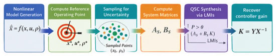
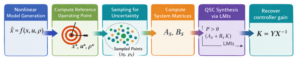
This workflow is illustrated in Figure 3, which summarizes the proposed sampling-based quadratic stability control framework. The diagram highlights the sequential process from nonlinear system modeling to robust controller synthesis.
Figure 3.
Flow diagram of the proposed sampling-based quadratic stability control pipeline. The procedure consists of nonlinear model generation, computation of a reference operating point, sampling over a neighborhood in state and parameter space, numerical evaluation of state and input matrices, and synthesis of a common state-feedback controller via Lyapunov-based LMIs. The circles schematically represent sampled state–parameter pairs; their colors and sizes are illustrative and do not encode quantitative information.
In particular, it emphasizes that all linearized models used for controller synthesis are generated by sampling a neighborhood of a dynamically feasible reference operating point. The sampled matrices represent local geometric and parameter variations. Their finite common certificate does not replace a proof over every nonlinear state and parameter value.
5.5. Experimental Setup
All performance studies use the same physical actuator ordering and signed feedback convention. The parameter sweeps use one QSC gain per setting; the uncertainty comparison uses five independently synthesized QSC gains at each uncertainty level. Both evaluate boundary/corner cases, and their results are reported separately to distinguish a single synthesis run from variation across runs. QSC is solved through CVX as a feasibility problem (zero objective), so it does not prescribe a unique feasible gain. For each completed trajectory of duration T, with position error , we use
Both metrics refer to the nominal reference; final position error is measured at simulation termination. Throughout, “Trajectory MSE” denotes this position-only time average and has units ; final position error has units . The integral is evaluated by trapezoidal quadrature on the adaptive ODE output times.
The lattice has four nominal 1 kg masses; axial/diagonal stiffnesses are 1/0.5 N/m, damping coefficients 1/0.5 N s/m and nominal spacing 1 m. Default settings are ; the parameter support is the relative componentwise box, and the state radius is in inherited numerical coordinates. The nominal LQR baseline minimizes the standard infinite-horizon quadratic cost with and ; its feedback gain is fixed when N or the synthesis radius varies.
Table 2 summarizes the nominal benchmark parameters and default design settings.
Table 2.
Nominal benchmark and default design settings. The state radius is defined in inherited numerical coordinates.
Here, “boundary/corner cases” refer to initial states sampled on the boundary of the state ball with parameter vectors at the corners of the relative parameter box. “Uniform cases” are sampled uniformly from the interior of the state ball and parameter box, while “stress cases” combine boundary states with corner parameters. “Common boundary/corner cases” denote a shared set of such samples used across all controllers in the comparison across five QSC gains.
Computational Environment
Controller synthesis uses MATLAB R2019b and CVX 2.2 [17] with SeDuMi [18], on an Apple M1 MacBook Air (8 cores, 8 GB; MATLAB maci64). Optimization times include CVX construction and solution, excluding plant/reference generation, sampling and verification. They are observed offline wall-clock times; only relative timings at the same sweep are directly comparable. Matrix dimension and constraint count, coefficient conditioning and solver settings can all affect time. Fixed N therefore does not imply constant time across radii or uncertainty levels.
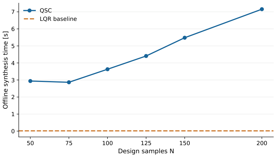
The offline SDP has scalar decision variables and stability blocks of order n. At , the observed wall-clock synthesis times for lattices with , 36 and 64 states were 2.3, 26.0 and 340.2 s, respectively. These times come from a separate scaling run on larger lattices, not from the tables above, and are not isolated hardware benchmarks.
For QSC, , and are imposed on the nominal model and N sampled models, with a zero objective. The value 8 is a fixed numerical bound retained from the original solver implementation, not a physical actuator limit or a value derived by optimizing the controller performance. It bounds the transformed decision variable Y, not the recovered gain K or the applied force; sensitivity to this chosen bound has not been evaluated.
5.6. Parameter and Actuation Sweeps
Each sweep entry uses one synthesis seed, 1000 random directions on the state-ball boundary and parameter-box corners under uncertainty, plus 1000 corresponding nominal cases per controller. The maximum integration horizon is 100 s; trajectories terminate earlier when the derivative norm falls below . Several sweep entries share baseline configurations. Trajectory MSE is evaluated over each actual duration; it is not an equal-horizon error integral.
5.6.1. Effect of the Number of Samples
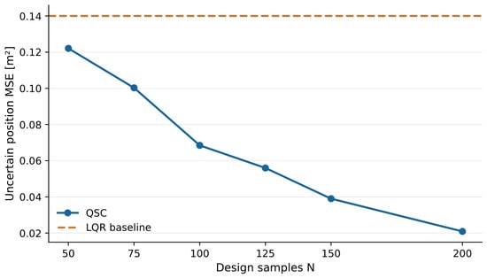
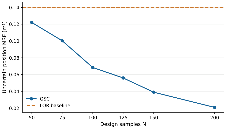
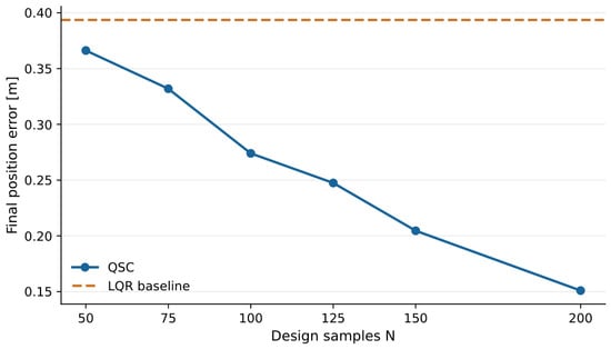
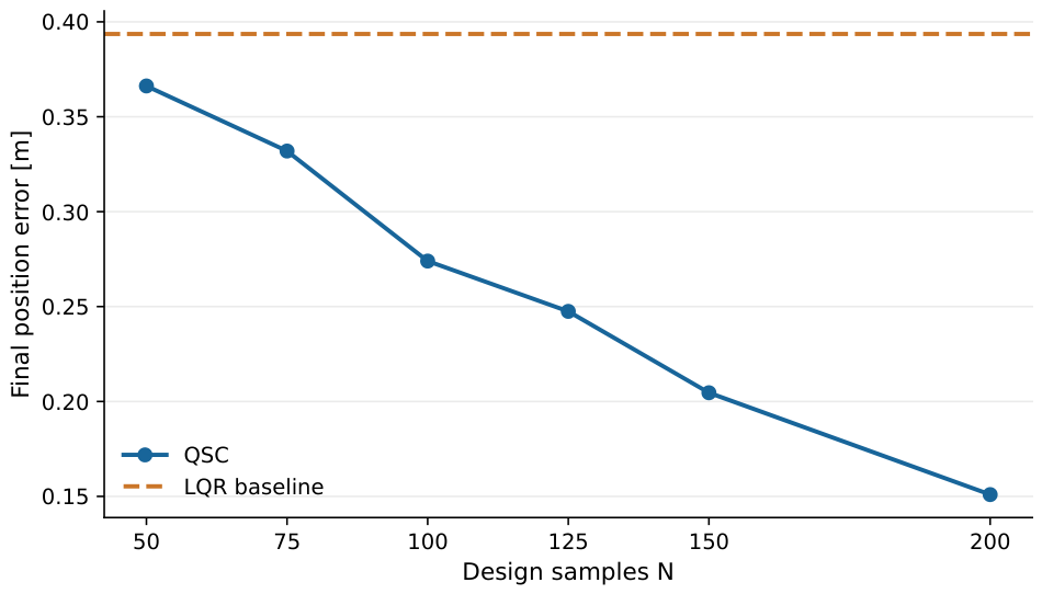
The sample-count sweep shows uncertain QSC trajectory MSE decreasing from 0.12210 at to 0.06848 at and 0.02093 at . The corresponding final position errors are 0.3662, 0.2740 and 0.1510 m. The observed trend is specific to this single-seed experiment. The nominal LQR gain is fixed across sample counts; its repeated evaluations yield the single baseline shown in Table 3 and the horizontal reference lines.
Table 3.
Sample-count sweep: QSC results for each N, with a single nominal unit-weight LQR baseline. The LQR gain is independent of N by construction. Means over 1000 cases per condition; time is offline synthesis time.
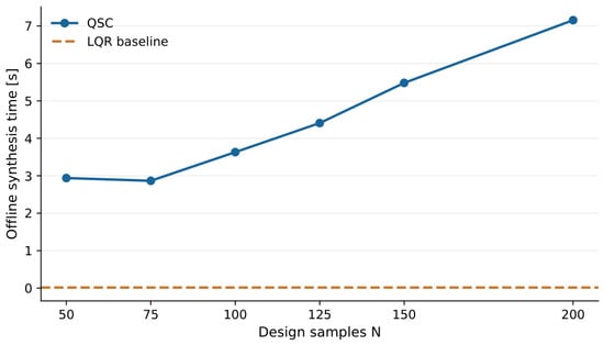
Figure 4, Figure 5 and Figure 6 show the corresponding uncertain trajectory MSE, final position error and offline synthesis time, respectively.
Figure 4.
Uncertain trajectory MSE versus sample count; single-seed synthesis and common boundary/corner test cases.
Figure 5.
Final position error versus sample count. These are measurements at simulation termination.
Figure 6.
Observed offline synthesis time versus sample count.
5.6.2. Effect of State Sampling Radius
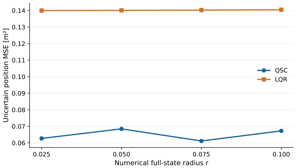
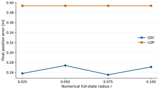
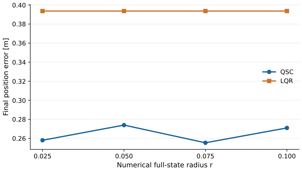
The radius changes both the synthesis region and initial deviations while keeping . Because state coordinates mix positions and velocities, r is a numerical radius, not a displacement-only physical radius. QSC uncertain final errors range from 0.2554 to 0.2740 m, while unit-weight LQR remains approximately 0.3936 m. Across the endpoints, QSC final position error increases by 5.01% and is 30.39–35.10% below LQR across the tested radii; uncertain trajectory MSE rises by 7.24% over the same range. These percentages are calculated from the unrounded data; variation across the four radii is nonmonotonic.
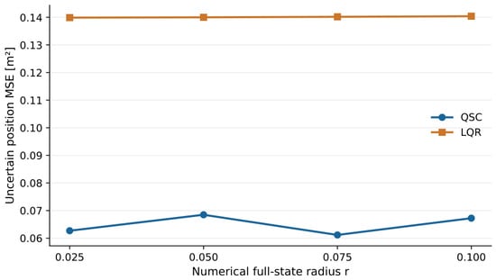
Table 4 reports the radius-sweep results, while Figure 7 and Figure 8 show the uncertain trajectory MSE and final position error, respectively.
Table 4.
Radius sweep; mean position-only metrics and observed offline synthesis time.
Figure 7.
Uncertain trajectory MSE versus numerical state radius.
Figure 8.
Final position error at simulation termination in metres; linear vertical axis. Means over 1000 uncertain boundary/corner cases.
In selected uncertain cases, the nominal reference has a nonzero acceleration residual of 0.810–1.266 , and longer integrations settle at a nonzero final position error. This offset is consistent with the parameter-induced reference residual of Section 4.3 and is limited to the tested cases.
5.6.3. Effect of Parameter Uncertainty
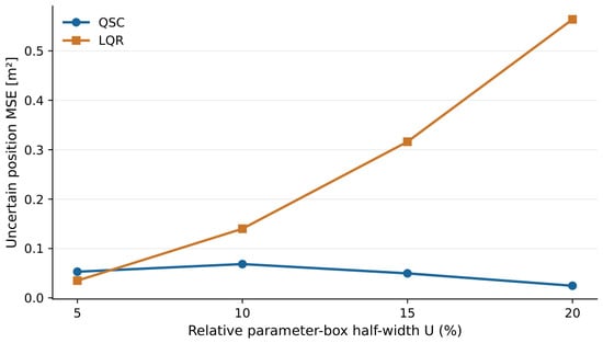
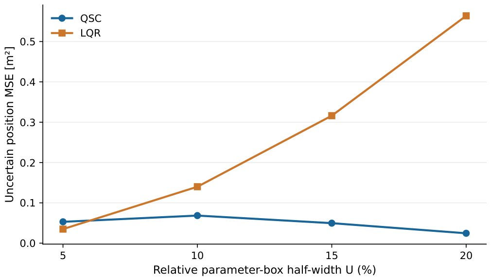
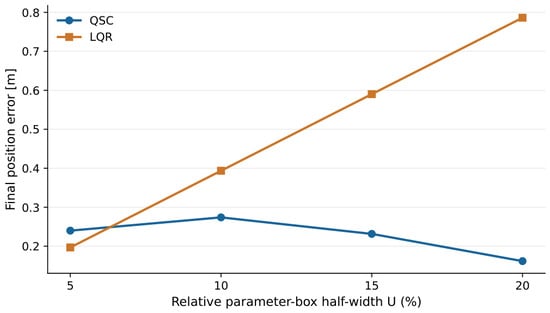
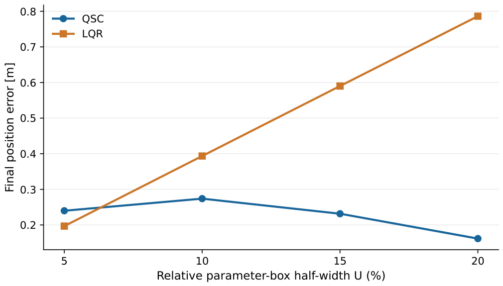
For this sweep the relative uncertainty width is used in both QSC synthesis and evaluation; a new sampled design is generated at each width. At , QSC trajectory MSE is 0.05302 versus 0.03492 for unit-weight LQR: QSC is worse in this case. At , the values are 0.02459 versus 0.56385, and final position errors are 0.1618 versus 0.7863 m. Thus, the benefit depends on uncertainty and on the selected gain.
Table 5 reports the uncertainty-sweep results; Figure 9 and Figure 10 show the corresponding uncertain trajectory MSE and final position error, respectively.
Table 5.
Uncertainty sweep; the uncertainty width changes synthesis and testing together.
Figure 9.
Uncertain trajectory MSE versus relative parameter-box width.
Figure 10.
Final position error versus relative parameter uncertainty.
5.6.4. Comparison Across Five Independently Synthesized Gains
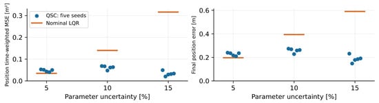
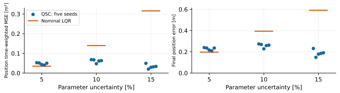
To test whether the low-uncertainty disadvantage is confined to one feasible gain, we repeat QSC synthesis with five independent random seeds (2–6), meaning five separately sampled state–parameter model families and five independently obtained QSC gains at each uncertainty level . For each seed we compare the resulting QSC gain with a nominal unit-weight LQR baseline on the same 1000 uncertain trajectories. The synthesis protocol uses SeDuMi with , , full actuation, reference seed 1 and validation seed 101. For evaluation, initial states lie on the ball boundary and uncertain parameter vectors are chosen from corners of the relative box. QSC synthesis uses the uniform sampling law of Section 4. The same initial states and normalized parameter draws are used across gains and uncertainty widths. Each gain is evaluated on 1000 nominal and 1000 uncertain trajectories. Fifteen QSC designs and three nominal LQR baselines give 36,000 trajectories.
Integration uses ode45 with relative and absolute tolerances and , a 100 s maximum horizon, and a derivative-norm stopping threshold . There is no clipping or external disturbance. Equation (28) is evaluated over each trajectory’s actual duration. Incremental force RMS is
aggregated over eight force channels.
At 5%, QSC has higher mean trajectory MSE, final position error and force RMS than paired nominal LQR in every synthesis seed. Relative increases are 15–52%, 7–22% and 57–90%, respectively. At 10% and 15%, QSC reduces both position-error metrics in every seed but uses more force. Table 6 gives averages of the test-case means obtained for each random seed; Figure 11 shows the individual seeds. The average MSE reductions at 10% and 15% are 56.0% and 89.5%, while force RMS is 4.56 and 7.26 times the LQR value.
Table 6.
Uncertainty comparison across five QSC gains: mean performance under parameter uncertainty. QSC spreads are standard deviations of the five means, each computed over the test cases for one random seed, not confidence intervals. Each seed mean uses 1000 cases.
Figure 11.
Uncertainty comparison across five QSC gains: five QSC seed means and nominal unit-weight LQR on the common uncertain test cases.
5.7. Effect of Actuator Configuration
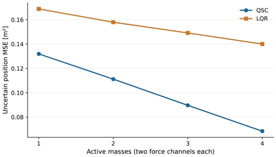
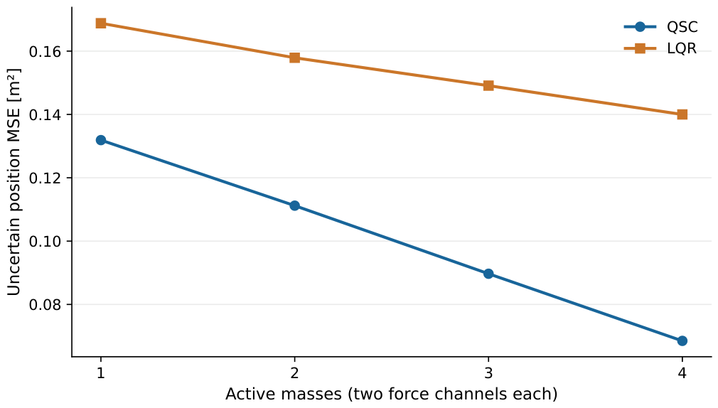
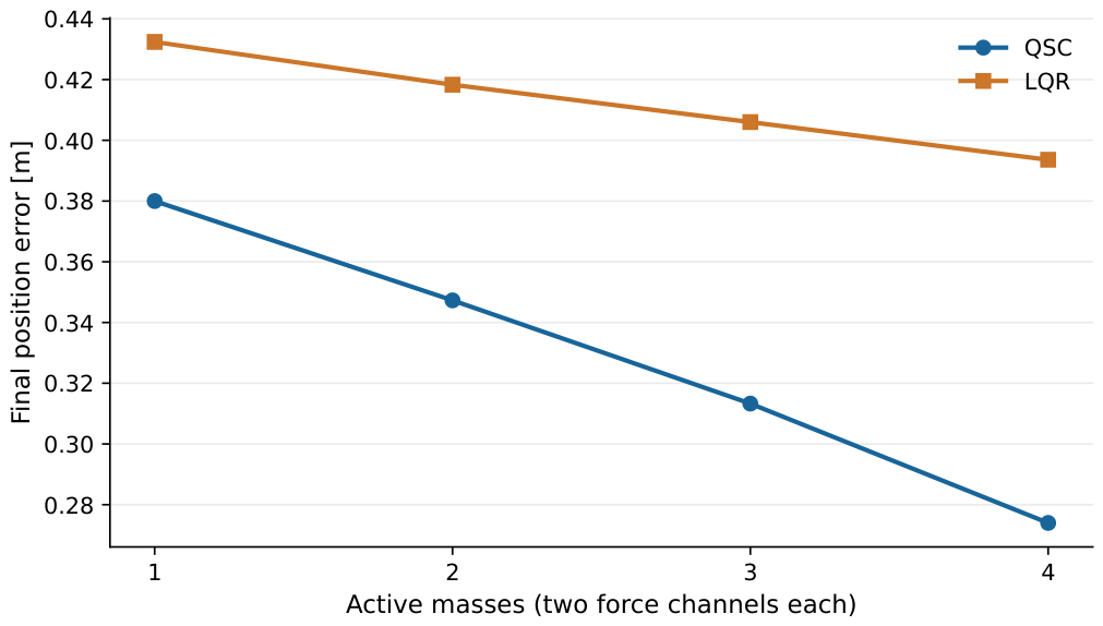
All 15 nonempty active-mass masks are evaluated, with two independent force components per active mass. Each mask uses , and ; controller performance is averaged over 1000 uncertain boundary/corner cases per mask. Means in Table 7 first average cases within a mask and then average masks of the same count. Each mask has its own feasible nominal reference, so this is not an isolated comparison at one identical reference. Aggregate errors decrease with additional active masses for both controllers. QSC is lower in both position metrics for all 15 tested masks. Actuator placement matters; these results apply to the tested configurations and references.
Table 7.
Performance under parameter uncertainty, averaged over actuator configurations with the same number of active masses.
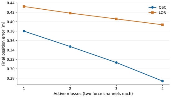
Figure 12 and Figure 13 show the trajectory MSE and final position error averaged across masks with the same number of active masses.
Figure 12.
Trajectory MSE averaged across masks with the same number of active masses.
Figure 13.
Final position error averaged across masks; each active mass has two force channels.
The comparison of synthesis sampling laws is reported in Appendix A.
6. Conclusions
Sampling-based QSC obtains one constant gain and a common quadratic Lyapunov matrix for a finite family of local Jacobians. For the nonlinear lattice, the simulations show that its regulation benefit relative to nominal unit-weight LQR depends on uncertainty, actuator placement and the selected feasible gain. Across five independently synthesized QSC gains, nominal LQR has lower position error and force effort at 5% uncertainty. QSC reduces both position-error measures at 10% and 15% in every tested seed, with substantially greater force effort. A stability-feasibility objective should therefore not be interpreted as an error or effort optimum.
Limitations and Future Work
The certificate covers the sampled homogeneous matrices and their convex hull. It does not establish stability across the entire continuous nonlinear domain. This distinction is relevant here: in the sampling-law study of Appendix A, the common Lyapunov matrix fails the homogeneous stability inequality at several independent boundary/corner Jacobians that were not used in synthesis. Parameter-dependent reference residuals also prevent an inference of exact reference regulation from homogeneous stability.
Appendix A provides the sampling-distribution study. All simulations reported in this manuscript are unsaturated: no force limits were applied, and clipping would change the closed-loop dynamics to which the unsaturated LMIs apply. The larger force effort of QSC at 10% and 15% uncertainty should therefore be checked against actuator ratings before any hardware use.
The experiments assume full-state feedback. With partial measurements, an observer and a joint controller–observer analysis would be needed to account for parameter mismatch, measurement noise and nonlinear estimation error; observer robustness is outside the present results.
The method may be useful for smooth coupled oscillators, discretized flexible structures and mechanical networks when local derivatives, state information and a feasible common-gain design are available. These are candidate applications, not validated benchmarks. Contact, hybrid and singular dynamics require separate treatment. Practical deployment should first use hardware-in-the-loop tests to assess delay, estimation noise, actuator bandwidth and force limits, followed by experiments on a small physical lattice. Further work should address performance-based selection among feasible gains, justified coordinate scaling, distribution-aware sampling, and nonlinear invariant-region and reference-offset bounds.
Author Contributions
Conceptualization, A.J.; methodology, A.J.; software, A.J.; validation, A.J. and Y.K.; formal analysis, A.J. and Y.K.; investigation, A.J.; resources, A.J.; data curation, A.J.; writing—original draft preparation, A.J.; writing—review and editing, A.J., S.S. and Y.K.; visualization, A.J.; supervision, S.S.; project administration, A.J.; funding acquisition, not applicable. All authors have read and agreed to the published version of the manuscript.
Funding
This research received no external funding.
Institutional Review Board Statement
Not applicable.
Informed Consent Statement
Not applicable.
Data Availability Statement
The implementation is available at https://github.com/AliJnadi/Quadratic-Stability-Control/ (accessed on 17 October 2026).
Acknowledgments
During preparation of this manuscript, the authors used ChatGPT (GPT-6.1 Sol) and OpenAI Codex (v0.163.0) to assist with language editing, code review and revision drafting. The authors reviewed the changes, independently checked the numerical results and take responsibility for the content.
Conflicts of Interest
The authors declare no conflicts of interest.
Abbreviations
The following abbreviations are used:
| CVX | Software for disciplined convex optimization in MATLAB |
| LMI | Linear Matrix Inequality |
| LQR | Linear Quadratic Regulator |
| MATLAB | Matrix Laboratory programming environment |
| MSE | Mean Squared Error |
| QSC | Quadratic Stability Control |
Appendix A. Sampling-Distribution Sensitivity
This appendix compares state-sampling distributions on the same nonlinear lattice benchmark.
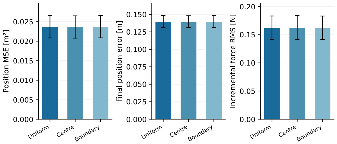
We compare three state-synthesis laws on the same numerical ball, with , five seeds and the same uniform-box parameter distribution. All laws share the saved uniform spherical directions, radial quantiles V and parameter/input draws. For , uniform-volume radius is ; the centre-biased law uses . Boundary enrichment is an equal mixture of uniform volume in the full ball and in the shell , implemented as
Each law retains full-ball support and uses the same parameter draws. Only the radial distribution, and hence the resulting sampled Jacobians, changes in the QSC LMIs. Five gains per law are evaluated on the same cases. All 15 designs satisfy the sampled synthesis constraints, and the trajectories under parameter uncertainty settle on the common 100 uniform and 32 boundary/corner validation cases per gain.
Centre-biased synthesis changes mean uniform-validation trajectory MSE by relative to uniform-volume synthesis; boundary enrichment changes it by . These small effects are specific to the tested support and five seeds. For each distribution and seed, the returned common Lyapunov matrix fails the homogeneous stability inequality at 4–5 independent boundary/corner Jacobians, although those closed-loop matrices have stable eigenvalues. The observed performance differences do not imply that sampling distribution is irrelevant.
Table A1 summarizes the validation metrics for the three sampling laws, and Figure A1 compares trajectory MSE on the common uniform validation cases.
Table A1.
Sensitivity to the sampling distribution used for synthesis: averages of the five test-case means, one for each random seed, on common validation sets under parameter uncertainty. Boundary denotes state-ball boundary samples with parameter-box corners.
Figure A1.
Sampling-law sensitivity on common uniform validation cases. Bars show averages of the five test-case means, one for each random seed; error bars show the standard deviations of these five means.
References
- Branicky, M.S. Multiple Lyapunov functions and other analysis tools for switched and hybrid systems. IEEE Trans. Autom. Control 1998, 43, 475–482. [Google Scholar] [CrossRef] [Scilit]
- Zhao, Z.; Wang, T.; Peng, F.; Yu, J. Adaptive Fuzzy Resilient Decentralized Control for Nonlinear Large-Scale CPSs Under DoS Attacks. IEEE Trans. Fuzzy Syst. 2024, 32, 5899–5909. [Google Scholar] [CrossRef] [Scilit]
- Vu, L.; Liberzon, D. Common Lyapunov functions for families of commuting nonlinear systems. Syst. Control Lett. 2005, 54, 405–416. [Google Scholar] [CrossRef] [Scilit]
- Slotine, J.J.E.; Li, W. Applied Nonlinear Control; Prentice Hall: Englewood Cliffs, NJ, USA, 1991. [Google Scholar]
- Aleksandrov, A.Y.; Chen, Y.; Kosov, A.A.; Zhang, L. Stability of Hybrid Mechanical Systems with Switching Linear Force Fields. Nonlinear Dyn. Syst. Theory 2011, 11, 53–64. [Google Scholar]
- Aleksandrov, A.Y.; Murzinov, I.E. On the Existence of a Common Lyapunov Function for a Family of Nonlinear Mechanical Systems with One Degree of Freedom. Nonlinear Dyn. Syst. Theory 2012, 12, 137–143. [Google Scholar]
- Boyd, S.; El Ghaoui, L.; Feron, E.; Balakrishnan, V. Linear Matrix Inequalities in System and Control Theory; Studies in Applied Mathematics; Society for Industrial and Applied Mathematics: Philadelphia, PA, USA, 1994; Volume 15. [Google Scholar] [CrossRef] [Scilit]
- Shorten, R.; Wirth, F.; Mason, O.; Wulff, K.; King, C. Stability Criteria for Switched and Hybrid Systems. SIAM Rev. 2007, 49, 545–592. [Google Scholar] [CrossRef] [Scilit]
- Oliveira, R.C.; Peres, P.L. Stability of polytopes of matrices via affine parameter-dependent Lyapunov functions: Asymptotically exact LMI conditions. Linear Algebra Its Appl. 2005, 405, 209–228. [Google Scholar] [CrossRef] [Scilit]
- Pipeleers, G.; Demeulenaere, B.; Swevers, J.; Vandenberghe, L. Extended LMI characterizations for stability and performance of linear systems. Syst. Control Lett. 2009, 58, 510–518. [Google Scholar] [CrossRef] [Scilit]
- Shamma, J.S.; Athans, M. Analysis of Gain Scheduled Control for Nonlinear Plants. IEEE Trans. Autom. Control 1990, 35, 898–907. [Google Scholar] [CrossRef] [Scilit]
- Leith, D.J.; Leithead, W.E. Survey of gain-scheduling analysis and design. Int. J. Control 2000, 73, 1001–1025. [Google Scholar] [CrossRef] [Scilit]
- Shimomura, T.; Kubotani, T. Gain-scheduled control under common Lyapunov functions: Conservatism revisited. In Proceedings of the 2005 American Control Conference, Portland, OR, USA, 8–10 June 2005; IEEE: Piscataway, NJ, USA, 2005; pp. 870–875. [Google Scholar]
- Calafiore, G.C.; Campi, M.C. The scenario approach to robust control design. IEEE Trans. Autom. Control 2006, 51, 742–753. [Google Scholar] [CrossRef] [Scilit]
- Campi, M.C.; Garatti, S.; Prandini, M. The scenario approach for systems and control design. Annu. Rev. Control 2009, 33, 149–157. [Google Scholar] [CrossRef] [Scilit]
- Campi, M.C.; Garatti, S. The exact feasibility of randomized solutions of uncertain convex programs. SIAM J. Optim. 2008, 19, 1211–1230. [Google Scholar] [CrossRef] [Scilit]
- Grant, M.; Boyd, S. CVX: MATLAB Software for Disciplined Convex Programming, Version 2.2. Software Documentation. 2026. Available online: https://cvxr.com/cvx (accessed on 7 October 2026).
- Sturm, J.F. Using SeDuMi 1.02, a MATLAB toolbox for optimization over symmetric cones. Optim. Methods Softw. 1999, 11, 625–653. [Google Scholar] [CrossRef] [Scilit]

Disclaimer/Publisher’s Note: The statements, opinions and data contained in all publications are solely those of the individual author(s) and contributor(s) and not of MDPI and/or the editor(s). MDPI and/or the editor(s) disclaim responsibility for any injury to people or property resulting from any ideas, methods, instructions or products referred to in the content. |
© 2026 by the authors. Licensee MDPI, Basel, Switzerland. This article is an open access article distributed under the terms and conditions of the Creative Commons Attribution (CC BY) license.