Simulation Analysis of the Dynamic Characteristics of the High-Speed Unloading Valve in the Back Pressure Assembly of an Injector Test System and Unloading Testing of the Valve

Abstract

Rapid pressure unloading is essential for the back pressure assembly of injector test systems. In this study, a high-speed unloading valve was developed for the back pressure assembly of an injector test system, and its pressure unloading characteristics were investigated through coupled numerical simulation and experimental testing. An electromagnetic–mechanical–fluid coupled dynamic model was established to describe the interactions among electromagnetic actuation, valve core motion, and hydraulic forces. Three-dimensional CFD simulations were performed to investigate the steady flow and hydraulic-force characteristics, followed by a two-dimensional transient model for analyzing the hydraulic force during valve closure. A coupled Simulink–AMESim model was then established to evaluate the system-level pressure unloading response and compared with experimental measurements under several initial pressure conditions. The CFD results reproduced the variation in flow rate with pressure differential, while sensitivity and uncertainty analyses showed that the quantified factors could not fully account for the discrepancy in absolute flow rate. Three-dimensional CFD revealed both axial and radial hydraulic forces, while 2D–3D comparison supported the use of the two-dimensional model for transient axial-force analysis. The system-level simulation and experimental results exhibited comparable pressure unloading characteristics within the investigated operating range.

1. Introduction

Accurate characterization of fuel injection rate is essential for the development, calibration, and performance evaluation of high-pressure common rail fuel injection systems. The injection rate profile provides direct information on the temporal evolution of fuel delivery and is therefore an important indicator for evaluating injector performance. Among the established measurement techniques, the Zeuch method determines the injection rate from the pressure variation in a measuring chamber and has been widely applied to the experimental characterization of fuel injection systems [1,2,3]. The measurement accuracy of the Zeuch method is affected by the hydraulic conditions of the measuring chamber and the characteristics of the pressure measurement system [2,3]. Therefore, precise control of the hydraulic boundary conditions of the measuring chamber is essential for obtaining reliable injection rate measurements.

In a Zeuch-type injector test system, the back pressure assembly provides the prescribed hydraulic boundary condition for the injector during the measurement process. The pressure variation in the measuring chamber is subsequently used to determine the injection rate characteristics [1,2,3]. In addition to maintaining the required back pressure, rapid pressure unloading after the measurement process is important for restoring the chamber to the required initial condition and preparing the system for the subsequent measurement cycle. Consequently, the pressure unloading capability of the back pressure assembly is an important functional requirement of an injector test system. In the conventional configuration considered in the present study, pressure unloading primarily relies on the injector-side flow path. To provide an independent and rapidly actuated unloading path, a dedicated high-speed unloading valve was therefore developed and integrated into the back pressure assembly of the injector test system.

High-speed on-off and solenoid valves have been extensively investigated for applications requiring rapid flow regulation and pressure control. Existing studies have examined the effects of valve geometry, structural parameters, throttling characteristics, and control strategies on the performance of high-speed on-off valves [4,5,6,7]. Meng et al. [4] established a mathematical model and investigated the influence of valve core diameter and seat angle on the flow force characteristics and linear control performance of a high-speed on-off valve. Mu et al. [5] developed and experimentally verified a linear high-speed on-off valve, demonstrating the influence of electromagnetic, mechanical, and transient hydraulic effects on valve motion. Wang et al. [6] investigated the hydraulic pressure characteristics of high-speed on-off valves, while Liu et al. [7] recently analyzed the flow field and throttling region of an electromagnetic high-speed on-off valve. These studies demonstrate that the dynamic performance of high-speed valves is closely associated with valve geometry, flow characteristics, and actuation behavior.

For applications requiring both rapid response and large transient flow capacity, Xu et al. [8] developed a three-stage fast-response directional valve and established a mathematical model considering both laminar and turbulent flow. The response process was divided into a starting delay and an opening process, and the influence of structural and control-pressure parameters on the dynamic response was investigated experimentally and numerically. In addition, transient CFD has been applied to investigate the dynamic characteristics of solenoid valves, including moving-valve flow fields, pressure-wave propagation, and transient pressure responses [9].

In parallel with high-speed switching valves, pressure relief and pressure-regulating valves have been studied from the perspective of transient flow, hydraulic forces, and valve motion. Manring and Zhang [10] experimentally investigated pressure-transient flow forces acting on hydraulic spool valves and showed that transient flow forces can be comparable in magnitude to steady-state flow forces. Three-dimensional CFD and experimental measurements have also been employed to determine the axial and normal flow forces acting on solenoid-operated spool valves, demonstrating the influence of asymmetric flow fields on the hydraulic forces acting on the spool [11]. More recently, CFD-based structural optimization has been applied to hydraulic spool valves to reduce steady-state flow forces and improve valve control characteristics [12]. For pressure-relief applications, Sang et al. [13] investigated the dynamic characteristics of a hydraulic poppet safety relief valve using a two-dimensional axisymmetric CFD model with dynamic mesh and UDF techniques. Their results demonstrated the effects of flow inertia, back pressure, and set pressure on the transient motion of the poppet. Experimental investigations of pressure-regulating poppet valves have further shown that valve motion, pressure fluctuation, and flow-induced instability are closely related to the dynamic interaction between the valve and the hydraulic system [14].

Previous studies have mainly focused on the intrinsic characteristics of individual valves, including opening and closing response, flow capacity, pressure regulation, flow force characteristics, and dynamic stability [4,5,6,7,8,9,10,11,12,13,14]. In contrast, the valve investigated in this study is designed specifically as a functional component of the back pressure assembly of an injector test system rather than as a general purpose high-speed switching or pressure-control valve. Its primary function is to provide an independent flow path for rapid pressure unloading. Therefore, the key performance indicator in the present application is the pressure-decay and unloading capability of the integrated back pressure assembly, rather than the isolated opening or closing time of the valve.

Another important issue in the dynamic analysis of high-speed valves is the interaction among electromagnetic actuation, valve core motion, and transient hydraulic forces. Studies of high-speed solenoid valves for common rail injectors have demonstrated the electromagnetic–mechanical–hydrodynamic multiphysics coupling associated with valve operation and have emphasized the influence of transient fuel hydrodynamic forces on valve dynamics [15].

Based on these considerations, this study develops a high-speed unloading valve specifically for the back pressure assembly of an injector test system and establishes an electromagnetic–mechanical–fluid coupled dynamic model. Three-dimensional CFD is used to characterize the steady-state flow and hydraulic-force characteristics, followed by two-dimensional transient CFD to investigate the hydraulic force during valve core closure. A coupled Simulink–AMESim model is then established to evaluate the system-level pressure unloading response, which is compared with experimental measurements under representative operating pressures. The objective is to develop an application-oriented modeling approach for rapid pressure unloading in injector test systems.

2. Structure and Operating Principle of the High-Speed Unloading Valve

The high-speed unloading valve investigated in this study was developed specifically for the back pressure assembly of an injector test system. The primary function of this valve is to provide an independent and rapidly actuated unloading flow path to reduce the pressure accumulated in the back pressure assembly after the injector measurement process. Therefore, unlike conventional proportional valves or pressure-regulating valves that focus on continuous flow adjustment, the proposed valve is designed as a high-speed on-off valve, where the main requirements are rapid actuation, reliable sealing, and sufficient unloading capacity.

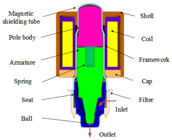
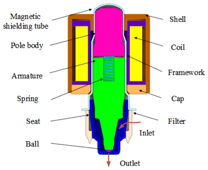
Figure 1 illustrates the structural configuration of the proposed high-speed unloading valve. The valve mainly consists of an electromagnetic actuator, moving armature, sealing ball, valve seat, return spring, and pole body. A steel ball is fixed at the end of the moving armature, and the armature and sealing ball are regarded as an integrated moving component during operation. The valve adopts a normally closed ball-seat sealing structure. Under the action of the spring preload, the sealing ball remains in contact with the valve seat when the electromagnetic coil is not energized, thereby maintaining the sealed state of the back pressure assembly and preventing unintended pressure leakage.

Figure 1. Schematic diagram of a high-speed pressure unloading valve.

When the electromagnetic coil is energized, the electromagnetic force generated by the actuator drives the moving armature and sealing ball away from the valve seat. The unloading passage is subsequently opened, allowing fuel to flow from the inlet port to the outlet port, and the pressure inside the back pressure assembly decreases rapidly. When the coil is de-energized, the electromagnetic force disappears, and the moving component returns to the closed position under the action of the spring force and hydraulic force. The normally closed configuration ensures that the valve can rapidly switch between the sealed state and unloading state according to the control signal.

Considering the requirements of rapid pressure unloading and reliable sealing in the injector test system, a ball-seat structure with a small moving stroke was selected. The relatively compact moving structure reduces the inertia of the moving components and facilitates rapid electromagnetic actuation. In addition, the sealing ball provides a stable sealing interface under the working pressure of the back pressure assembly. It should be noted that the objective of this study is not to optimize the valve geometry for flow regulation characteristics, but to investigate the dynamic unloading behavior of the valve when integrated into the back pressure assembly.

The main structural parameters of the proposed valve are summarized in Table 1. These parameters mainly determine the sealing reliability, maximum flow passage area, and structural manufacturing accuracy of the valve. During the flow capacity evaluation, the valve was considered to be fully opened, corresponding to the maximum unloading condition of the back pressure assembly.

Table 1. Main structural parameters of the high-speed unloading valve.

Parameter	Symbol	Nominal Value	Manufacturing Tolerance
Maximum valve stroke	xmax	0.25 mm	±0.02 mm
Seat cone angle	θ	105°	±2°
Inlet diameter	Dinlet	0.65 mm	±0.02 mm
Outlet diameter	Doutlet	0.8 mm	±0.02 mm
Sealing ball diameter	Dball	1.5 mm	±0.02 mm
Coil turns	N	420	-

3. Mathematical Model of the Unloading Valve

3.1. Dynamic Model of the Valve Core

In the present study, the armature and sealing ball are regarded as an integrated moving component, and only its axial motion is considered. According to Newton’s second law, the axial motion of the valve core can be described as follows:

$$m {\displaystyle \frac{{\partial }^{2}x}{\partial t^2}}=F_{\mathit{Mag}}-F_{\mathit{Hyd}}-F_{\mathit{Spr}}-F_f-F_{\mathit{mg}},$$

(1)

where m is the equivalent mass of the moving component, x is the axial displacement of the valve core, t is the motion duration, F_Mag is the electromagnetic force, F_Hyd is the hydraulic force, F_Spr is the spring force, F_f is the mechanical friction force, and F_mg is the gravitational force. During operation, the valve core is completely immersed in the test oil, and the moving distance is only 0.25 mm. Therefore, the mechanical friction is considered to be small because of the oil-lubricated working environment. In addition, the mass of the moving component is approximately 0.004 kg, corresponding to a gravitational force of only about 0.04 N. Compared with the electromagnetic, hydraulic, and spring forces acting on the valve core, both friction and gravity are considered secondary effects and are neglected in the subsequent dynamic model. Equation (1) is therefore simplified to

$$m {\displaystyle \frac{{\partial }^{2}x}{\partial t^2}}=F_{\mathit{Mag}}-F_{\mathit{Hyd}}-F_{\mathit{Spr}},$$

(2)

The positive direction of x is defined as the direction in which the valve core moves away from the valve seat. Thus, the electromagnetic force acts in the positive direction during valve opening, whereas the spring force and hydraulic force are taken as resistance terms according to the adopted coordinate convention.

The hydraulic force acting on the valve core is obtained from the pressure and viscous shear stresses on the wetted surface. Its axial component can be calculated as follows:

$$F_{\mathit{Hyd}}=-\left[{\displaystyle {\int }_S(-pn+\tau ·n)\mathit{dS}}\right]e_x,$$

(3)

where S is the wetted surface of the valve core, p is the local pressure, n is the outward normal vector, τ is the viscous stress tensor, and e_x is the unit vector in the positive x-direction. The axial hydraulic force used in the valve core dynamic equation is obtained by projecting the resultant hydraulic force onto the valve axis.

Unlike a constant hydraulic-force approximation, the present model obtains the hydraulic force directly from the CFD-calculated pressure and velocity fields.

3.2. Electromagnetic Force Model

The electromagnetic force on the armature can be expressed as follows:

$$F_{\mathit{mag}}={\displaystyle \frac{{\left(\mathit{NI}\right)}^2{\mu }_0}{2K_f^2{\delta }^2}}{A}_m,$$

(4)

where μ₀ is the vacuum permeability, A_m is the effective magnetic pole area, δ is the air gap of the armature, I is the current on the coil, N is the number of coil turns, and K_f is the magnetic flux leakage factor.

Equation (4) provides an idealized relationship between electromagnetic force, coil current, and air gap. Because the actual actuator has a nonlinear magnetic circuit, the electromagnetic force used in the coupled model was obtained from ANSYS Maxwell 2022 using the experimentally measured B–H characteristics. The resulting electromagnetic characteristics were expressed in the form

F_mag = f(I,δ),

(5)

The resulting electromagnetic force map was subsequently introduced into the system-level dynamic model, allowing the electromagnetic force to vary with both the coil current and the instantaneous air gap.

3.3. Spring Force Model

The return spring provides the restoring force required to return the valve core to the valve seat after the electromagnetic actuator is de-energized. Assuming linear spring behavior, the spring force is expressed as:

F_Spr = F₀ + kx,

(6)

where F₀ is the preload of the spring at the closed position and k is the spring stiffness.

For the investigated valve, the spring preload at the closed position is 2.6 N, while the spring stiffness is 1170 N/m. The maximum valve core displacement is 0.25 mm. Therefore, when the valve core reaches the fully open position, the spring reaction force is

F_Spr,max = F₀ + kx_max,

(7)

Substituting the corresponding parameters gives

F_Spr,max = 2.6 + 1170 × 0.25 × 10⁻³ ≈ 2.9 N,

(8)

Thus, the 2.6 N and 2.9 N values correspond to different valve core positions: 2.6 N is the spring preload when the valve is closed, whereas approximately 2.9 N is the spring reaction force when the valve is fully open.

3.4. Flow Model

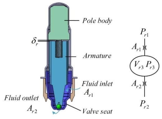
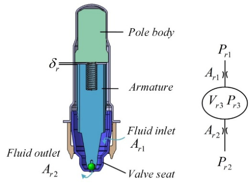
The flow through the two characteristic throttling sections can be described using the orifice-flow relationship shown in Figure 2.

Figure 2. Orifice-flow simplification of the unloading valve.

For the first section,

$$Q_r=C_d{A}_{r1}\sqrt{{\displaystyle \frac{2\left(P_{r1}-P_{r3}\right)}{\rho }}},$$

(9)

and for the second section,

$$Q_r=C_d{A}_{r2}\sqrt{{\displaystyle \frac{2\left(P_{r3}-P_{r2}\right)}{\rho }}},$$

(10)

where P_r1 and P_r2 are the inlet and outlet pressure of the valve, A_r1 and A_r2 are the inlet and outlet throttle cross-sectional area, Q_r is the flow rate, P_r3 is the intermediate pressure, ρ is the fluid density, and C_d is the flow coefficient.

Because the two throttling sections are connected in series, the intermediate pressure P_r3 can be eliminated, giving

$$Q_r=C_d{\displaystyle \frac{A_{r1}{A}_{r2}}{\sqrt{A_{r1}^2+A_{r2}^2}}}\sqrt{{\displaystyle \frac{2\left(P_{r1}-P_{r2}\right)}{\rho }}},$$

(11)

Equation (11) is used to describe the relationship between the pressure differential and flow capacity of the valve.

3.5. Model Parameters and Main Assumptions

To formulate the coupled dynamic model while limiting model complexity, the following assumptions are made:

(1)

One-dimensional valve core motion: only axial valve core motion is considered in the mechanical model.

(2)

Electromagnetic characteristics: the electromagnetic force is represented by the Maxwell-calculated force map F_mag = f(I,δ), based on the measured magnetic B-H characteristics.

(3)

Hydraulic force: the hydraulic force acting on the valve core is obtained from the CFD pressure and viscous stress distributions rather than assuming a constant flow force coefficient.

(4)

Mechanical friction and gravity: because the valve core is fully immersed in oil and has a very short stroke, mechanical friction and gravity are considered secondary effects and are neglected in the dynamic equation.

(5)

Working fluid: the working fluid is No. 0 diesel at ambient temperature, consistent with the operating conditions of the back pressure assembly. Its density and dynamic viscosity are treated as constant.

(6)

Steady flow-capacity analysis: the valve is considered fully open when evaluating its steady-state flow capacity.

(7)

Transient closure: the transient CFD model is initialized with the valve fully open and simulates the process of valve core closing from x = x_max to x = 0, thereby obtaining the transient flow-field evolution and hydraulic force.

3.6. Coupling Strategy of the Electromagnetic, Mechanical, and Fluid Models

The electromagnetic, mechanical, and fluid characteristics are coupled to establish the dynamic model of the unloading valve. The overall coupling relationship can be represented as

I(t) → F_Mag(I,δ) → x(t) → Q(t) → P(t),

(12)

where the electromagnetic force is determined by the coil current and instantaneous air gap, while the resulting valve core motion affects the hydraulic state of the valve.

The hydraulic pressure and flow field subsequently determine the hydraulic force acting on the valve core:

Q(t),P(t) → F_Hyd(t) → x(t),

(13)

The electromagnetic force characteristics obtained from Maxwell and the hydraulic-force characteristics obtained from CFD are incorporated into the Simulink–AMESim coupled model. AMESim is used to represent the oil chamber, unloading valve, mass block, and displacement limiter, while Simulink implements the electromagnetic force and fluid-force relationships.

4. Electromagnetic Simulation Analysis

4.1. Electromagnetic Model and Material Properties

The electromagnetic actuator provides the driving force required for the valve core to move away from the valve seat. An electromagnetic simulation was performed in ANSYS Maxwell to obtain the force characteristics required by the coupled dynamic model.

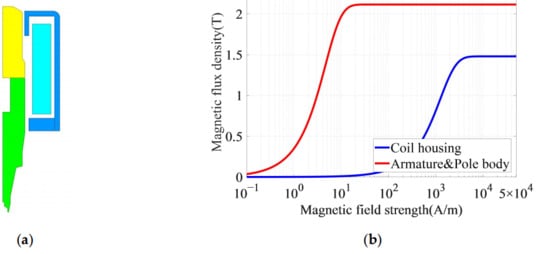
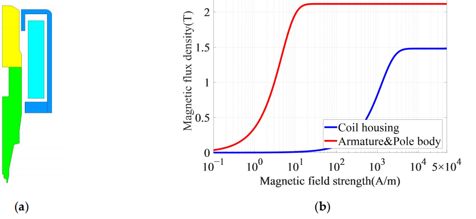
To reduce the computational cost while retaining the main characteristics of the electromagnetic field, the electromagnetic structure of the valve was simplified and a two-dimensional axisymmetric electromagnetic model was established in ANSYS Maxwell, as shown in Figure 3a. The central regions represent the pole body and armature, while the outer regions represent the coil windings and coil housing.

Figure 3. Simulation preparations: (a) Electromagnetic simulation model; (b) The B-H curves.

The nonlinear magnetic properties of the materials were considered in the electromagnetic simulation. The B-H characteristics of the pole body, armature, and coil housing were experimentally obtained, as shown in Figure 3b, and subsequently imported into ANSYS Maxwell. Therefore, the magnetic properties of the actual materials were incorporated into the electromagnetic simulation.

According to the design parameters of the unloading valve, the coil current was varied from 0 to 3 A, while the air gap was varied from 0 to 0.25 mm. The selected air-gap range corresponds to the maximum designed valve core displacement, while the current range covers the operating range of the electromagnetic actuator. The electromagnetic force was calculated for the corresponding combinations of coil current and air gap.

4.2. Electromagnetic Force Characteristics

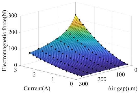
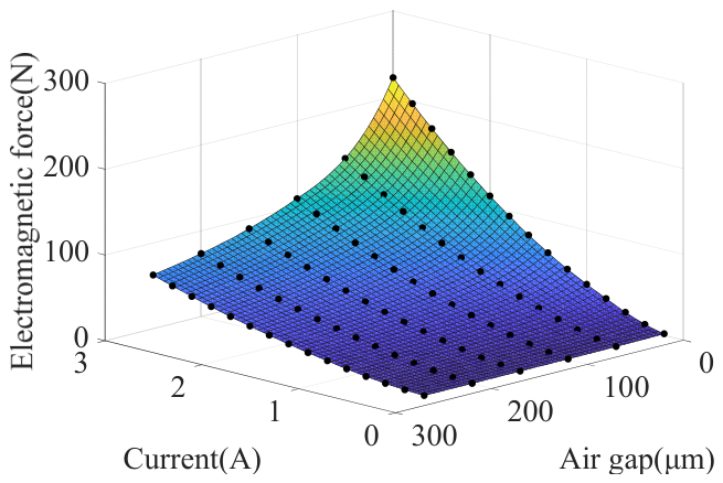
The calculated electromagnetic force characteristics are presented in Figure 4. As shown in Figure 4, the electromagnetic force increases with coil current and decreases with air gap. The resulting force map was used in the subsequent coupled simulation.

Figure 4. The relationship between electromagnetic force, drive current and operating air gap.

4.3. Electromagnetic Force Requirement Under the Design Condition

To evaluate whether the electromagnetic actuator provides sufficient driving force under the designed operating condition, a pressure differential of 10 MPa was considered as an example.

When the valve is in the normally closed position, the spring preload is 2.6 N. Under the 10 MPa pressure differential, the hydraulic force acting on the valve core is approximately 7.3 N according to the force analysis. Since the effects of mechanical friction and gravity are neglected in the dynamic model, the electromagnetic force required to initiate valve core opening should satisfy

F_Mag > F_Hyd + F_Spr,

(14)

Therefore, under a pressure differential of 10 MPa,

F_Mag > 7.3 + 2.6 = 9.9 N,

(15)

According to the electromagnetic simulation results shown in Figure 4, the electromagnetic force exceeds approximately 10 N when the coil current reaches about 1.2 A under the corresponding air-gap condition. Thus, the electromagnetic actuator provides sufficient driving force to overcome the hydraulic and spring forces under the designed pressure condition and initiate valve core opening.

The Maxwell simulation therefore serves two purposes in the present study. First, it provides the electromagnetic force characteristics required for the coupled electromagnetic–mechanical–fluid model. Second, the force-balance analysis confirms that the designed electromagnetic actuator has sufficient driving capability under the specified operating pressure.

5. CFD Analysis of the Unloading Valve

5.1. Three-Dimensional CFD Model and Boundary Conditions

A three-dimensional computational fluid dynamics (CFD) model of the internal flow passage of the high-speed unloading valve was established to investigate its steady-state flow characteristics and hydraulic forces under different pressure differentials. The computational domain was constructed according to the actual internal geometry of the valve, including the inlet passage, valve seat, valve core region, and outlet passage. The central hollow region of the valve body was retained in the fluid domain to reproduce the actual flow passage. The valve core was considered to be fully open during the steady-state flow analysis.

A polyhedral mesh was employed for the three-dimensional fluid domain to improve mesh quality and computational efficiency. Considering the relatively high velocity gradients in the throttling region, local mesh refinement was applied around the valve orifice and the adjacent flow passage. A refined boundary layer mesh was also generated near the solid walls to better resolve the near-wall flow characteristics. Based on preliminary mesh tests, the maximum element size in the main flow region was set to 0.1 mm, while the minimum local element size in the refined region was set to 0.008 mm. The resulting medium mesh contained 1,076,300 cells. The influence of mesh density on the predicted flow rate and hydraulic forces was subsequently evaluated using three mesh resolutions, as discussed in Section 5.2.

Because of the strong pressure and velocity gradients in the throttling region, the k-ω SST model was selected as the primary turbulence model for the steady-state CFD simulations. The curvature correction and production limiter were enabled to account for the effects of streamline curvature in the complex internal flow field. The standard k-ε model was additionally employed under the same operating conditions to assess the sensitivity of the predicted flow characteristics and hydraulic forces to the turbulence model selection. The comparison between the two turbulence models is presented in Section 5.2.

Pressure boundary conditions were prescribed at the inlet and outlet of the computational domain. The inlet pressure was successively set to 2, 5, 8, 10, 12, and 15 MPa, while the outlet pressure was maintained at 0 MPa gauge pressure. Therefore, the investigated pressure-differential range was 2–15 MPa. These operating conditions correspond to the pressure range considered in the steady-state flow-capacity evaluation of the unloading valve.

The working fluid was No. 0 diesel fuel at ambient temperature, consistent with the actual operating conditions of the injector test system. The fluid density and dynamic viscosity used in the CFD model were 840 kg/m³ and 0.0038 Pa∙s, respectively. The same fluid properties were maintained for all investigated pressure differentials.

A pressure-based solver was employed for the steady-state calculations, and the residual convergence criterion was set to 1 × 10⁻⁶. The calculations were continued until the monitored flow variables and hydraulic forces reached stable values. The converged three-dimensional steady-state flow fields were subsequently used to evaluate the unloading flow rate and the axial and radial hydraulic forces acting on the valve core.

5.2. Grid Independence and Turbulence Model Sensitivity

To assess the numerical reliability of the three-dimensional CFD model, a grid-independence analysis was conducted at a pressure differential of 10 MPa using coarse, medium, and fine meshes. The predicted flow rate and the axial and radial hydraulic forces were selected as the evaluation parameters. The results obtained with the k-ω SST model are summarized in Table 2. When the mesh was refined from medium to fine, the flow rate and axial hydraulic force changed by only 1.01% and 0.85%, respectively, while the radial hydraulic force changed by 5.71%. These results indicate that further mesh refinement has a limited effect on the predicted flow rate and axial hydraulic force.

Table 2. Grid-independence and turbulence model sensitivity results at 10 MPa.

Turbulence Model	Mesh	Number of Cells	Flow Rate (L/min)	Axial Hydraulic Force (N)	Radial Hydraulic Force (N)
k-ω SST	Coarse	629,454	1.98	2.46	0.9
k-ω SST	Medium	1,076,300	1.96	2.34	0.66
k-ω SST	Fine	1,639,406	1.98	2.36	0.7
Standard k-ε	Coarse	629,454	2.01	2.41	0.89
Standard k-ε	Medium	1,076,300	1.986	2.36	0.689
Standard k-ε	Fine	1,639,406	1.986	2.35	0.65

The sensitivity to the turbulence model selection was then evaluated using the standard k-ε model under the same mesh resolutions and boundary conditions. From the medium to the fine mesh, the changes in flow rate and axial hydraulic force were 0% and 0.43%, respectively, while the radial hydraulic force changed by approximately 6.0%. Using the medium mesh, the differences between the k-ω SST and standard k-ε models were 1.31% for flow rate, 0.85% for axial hydraulic force, and 4.21% for radial hydraulic force. For the fine mesh, the corresponding differences were approximately 0.30%, 0.43%, and 7.69%, respectively. Overall, the predicted flow characteristics and axial hydraulic force show limited sensitivity to both mesh resolution and turbulence model selection under the investigated condition.

Based on these results, the medium mesh was adopted for the subsequent three-dimensional simulations as a compromise between numerical accuracy and computational cost, while the k-ω SST model was selected as the primary turbulence model. The standard k-ε model was retained for comparison in the sensitivity analysis. It should also be noted that the radial hydraulic force is not negligible compared with the axial component. At 10 MPa, the radial-to-axial hydraulic-force ratio obtained with the medium mesh and k-ω SST model is approximately 28.2%. Therefore, the three-dimensional model was retained for evaluating the complete hydraulic-force characteristics, whereas the subsequent transient analysis focuses on the axial motion of the valve core. The applicability of the two-dimensional transient model is further examined in Section 5.5 by comparing its axial hydraulic force with the corresponding three-dimensional results.

5.3. Steady-State Flow Characteristics and Experimental Validation

5.3.1. Comparison of CFD and Experimental Flow Rates

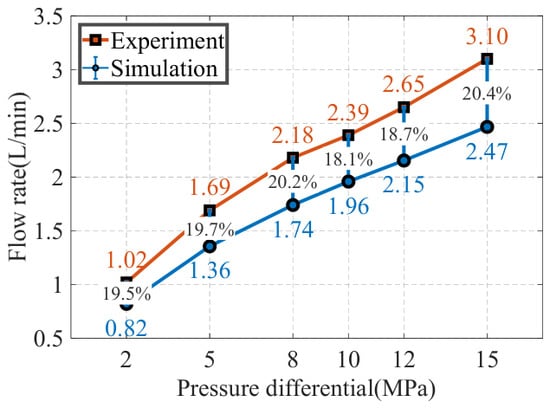
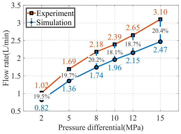
To evaluate the steady-state flow characteristics of the high-speed unloading valve, simulations were conducted under inlet pressures of 2, 5, 8, 10, 12, and 15 MPa, with the outlet pressure maintained at 0 MPa gauge pressure. The valve was assumed to be fully open under all steady-state conditions. The simulated and experimental flow rates are compared in Figure 5.

Figure 5. Comparison of simulated and experimental flow rates under different pressure differentials.

The flow rate increases with pressure differential in both the CFD and experimental results, indicating that the CFD model captures the overall pressure-flow trend. However, the CFD results consistently underpredict the experimental flow rates, with relative deviations ranging from 18.1% to 20.4% over the investigated pressure range. For example, at a pressure differential of 10 MPa, the simulated and experimental flow rates are 1.96 and 2.39 L/min, respectively, corresponding to a deviation of approximately 18%.

The observed discrepancy in absolute flow rate is further examined through geometric sensitivity, numerical sensitivity, and measurement-uncertainty analyses in Section 5.3.2 and Section 5.3.3.

5.3.2. Sensitivity and Uncertainty Analysis

To further quantify the potential sources of discrepancy between the CFD and experimental results, sensitivity analyses were performed for the main geometric, numerical, and measurement-related factors. Since the valve was fully open during the steady-state flow-rate tests, the effects of the inlet and outlet diameters were evaluated using the equivalent serial-orifice relationship given in Equation (11). The nominal inlet and outlet diameters were 0.65 and 0.80 mm, respectively, with a manufacturing tolerance of ±0.02 mm. Considering the four combinations of the upper and lower tolerance limits of the two diameters, the calculated flow-rate variation relative to the nominal geometry ranged from −5.72% to +5.88%, corresponding to a maximum variation of approximately 5.9%. This result indicates that the dimensional tolerances of the two serial flow restrictions can have a noticeable influence on the predicted flow rate.

In addition to geometric tolerance, the numerical sensitivity results obtained in Section 5.2 are included for comparison. The medium-to-fine mesh difference in flow rate is approximately 1.01% for the k-ω SST model, while the difference between the k-ω SST and Standard k-ε models is approximately 1.31% for the medium mesh. These numerical effects are substantially smaller than the observed 18.1–20.4% CFD–experimental deviation.

The uncertainty of the experimental measurements was also evaluated according to the specifications of the measurement instruments. The hydraulic pressure sensor has a measuring range of 0–300 bar and an accuracy of ±0.1% full scale, corresponding to an absolute uncertainty of ±0.30 bar. The flow sensor has a measuring range of 0.004–4 L/min and an accuracy of ±0.2% full scale, corresponding to an absolute uncertainty of ±0.008 L/min. For the experimental flow-rate range of 1.02–3.10 L/min, this corresponds to a relative flow-rate uncertainty of approximately ±0.26–0.78%.

The quantified factors are summarized in Table 3.

Table 3. Quantitative assessment of the main identified sources of CFD–experimental discrepancy.

Factor	Evaluation Approach	Quantitative Assessment
Combined tolerance of the two serial orifices	Equation (11)	−5.72% to +5.88%
Mesh resolution	Medium-to-fine	≈1.01%
Turbulence model	k-ω SST vs. Standard k−ε	≈1.31%
Flow-rate measurement	0.004–4 L/min, ±0.2% FS	±0.008 L/min (≈±0.26–0.78%)
Pressure measurement	0–300 bar, ±0.1% FS	±0.30 bar

The dimensional sensitivity values represent potential flow-rate variations within the specified tolerance range and do not represent the actual contribution of dimensional errors to the CFD–experimental discrepancy.

5.3.3. Analysis of the CFD–Experimental Deviation

As shown in Figure 5, the CFD results consistently underpredict the experimental flow rates over the investigated pressure range, with deviations of approximately 18.1–20.4%. The sensitivity analysis indicates that the combined tolerance of the two serial orifices can produce a flow-rate variation of up to approximately 5.9%, whereas the effects of mesh resolution, turbulence model selection, and measurement uncertainty are comparatively small. Therefore, the quantified factors alone cannot fully account for the observed difference between the CFD and experimental results.

Because the remaining potential influences were not independently measured or quantified in the present study, their individual contributions cannot be reliably identified. Therefore, no arbitrary percentage allocation or specific causal attribution of the remaining discrepancy is introduced. The present analysis instead identifies the quantitatively assessable sources of uncertainty and clarifies the limitations of the current CFD–experimental comparison. Despite the difference in absolute flow rate, the CFD results reproduce the variation in flow rate with pressure differential and provide a consistent basis for the subsequent hydraulic-force and transient-flow analyses.

5.4. Three-Dimensional Hydraulic Force Characteristics

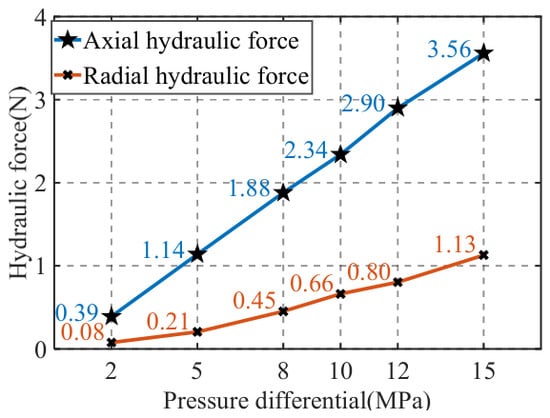
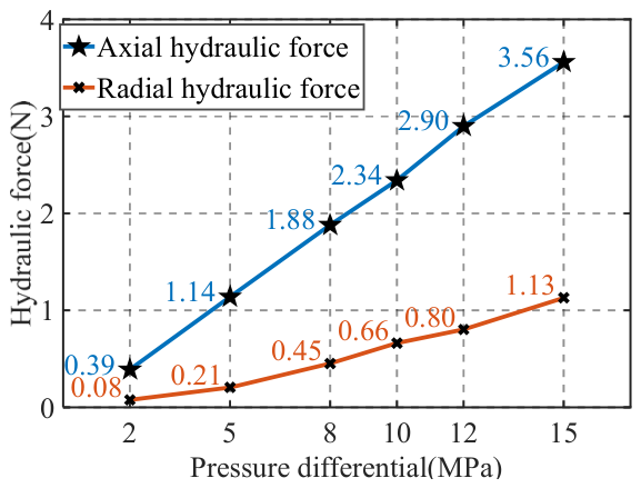
The three-dimensional CFD results for the fully open valve are shown in Figure 6. The axial hydraulic force always acts in the valve-closing direction, which is opposite to the positive x-direction defined in Section 3.1. When the valve core is fully open, the spherical head is located close to the outlet passage. The relatively high flow velocity around the spherical head produces a low-pressure region, resulting in a net axial force toward the valve seat. With increasing pressure differential, the magnitude of the axial hydraulic force increases from 0.39 N at 2 MPa to 3.56 N at 15 MPa. At the design pressure differential of 10 MPa, the axial hydraulic force reaches 2.34 N.

Figure 6. Axial and radial hydraulic forces at different pressure differentials.

Because the valve has a single asymmetric inlet passage, the pressure and velocity distributions around the valve core are asymmetric in the radial direction, producing a radial hydraulic force. The radial force increases from 0.08 to 1.13 N over the investigated pressure range and reaches 0.66 N at 10 MPa. At this condition, the radial-to-axial force ratio is approximately 28.2%, indicating that the radial component is not negligible and should be considered when evaluating the complete three-dimensional hydraulic loading.

In the present mechanical configuration, the valve core is constrained to one translational degree of freedom along the valve axis. Therefore, the subsequent transient analysis focuses on the axial hydraulic force during valve core closure. The applicability of the two-dimensional transient model is further evaluated in Section 5.5 by comparing its axial hydraulic force with the corresponding three-dimensional results.

5.5. Two-Dimensional Transient CFD Model and 2D/3D Validation

To investigate the variation in the hydraulic force during valve core motion, a two-dimensional axisymmetric flow model was established for the subsequent transient analysis. The simplification was introduced primarily to enable efficient moving-mesh simulation while retaining the dominant axial flow characteristics associated with valve closure. As discussed in Section 5.4, the three-dimensional valve flow field exhibits a non-negligible radial hydraulic force because of the asymmetric single-inlet configuration. Therefore, the applicability of the two-dimensional model was further evaluated by comparing its predicted axial hydraulic force with that obtained from the three-dimensional model.

The two-dimensional fluid domain was discretized using a mesh with a characteristic cell size of 0.02 mm. The mesh contained 84,288 cells and 86,109 nodes. The minimum orthogonal quality was 0.58, with an average value of 0.99, while the maximum skewness was 0.75 and the average value was 0.017. These mesh-quality indicators satisfy the requirements for the subsequent transient moving-mesh calculation.

Before switching to the transient calculation, 400 iterations of steady-state flow-field calculations were performed to obtain a stabilized initial flow field. The axial hydraulic forces obtained from the stabilized two-dimensional flow field were then compared with the corresponding three-dimensional steady-state results presented in Section 5.4. The comparison is summarized in Table 4.

Table 4. Comparison of axial hydraulic forces predicted by the 2D and 3D models.

Pressure Differential (MPa)	3D Axial Force (N)	2D Axial Force (N)	Relative Difference
2	0.39	0.40	2.56%
5	1.14	1.10	3.51%
8	1.88	1.80	4.26%
10	2.34	2.30	1.71%
12	2.90	2.80	3.45%
15	3.56	3.50	1.69%

As shown in Table 4, the axial hydraulic forces predicted by the two-dimensional model are in close agreement with those obtained from the three-dimensional model over the entire investigated pressure range. The relative differences are between 1.69% and 4.26%, with an average difference of approximately 2.86%. At the design pressure differential of 10 MPa, the axial hydraulic forces predicted by the 3D and 2D models are 2.34 and 2.30 N, respectively, corresponding to a difference of only 1.71%.

The comparison demonstrates that, although the asymmetric three-dimensional flow field generates a non-negligible radial hydraulic force, the resulting difference in the predicted axial hydraulic force remains limited for the present valve geometry and operating conditions. Since the valve core is mechanically constrained to one translational degree of freedom along the valve axis, the axial hydraulic force is the relevant hydraulic-force component governing the subsequent closing motion. Therefore, the two-dimensional model is considered appropriate for the transient analysis of the valve core closing process within the investigated pressure range. This approach reduces the computational cost of the moving-core simulation while retaining the axial hydraulic-force characteristics required for the dynamic analysis.

After the stabilized steady-state calculation, the flow field was switched to transient mode. The k-ω SST turbulence model was retained, with the production limiter enabled. Dynamic mesh motion was implemented using the smoothing and local mesh-reconstruction methods. The minimum and maximum length scales for mesh reconstruction were set to 0.015 and 0.025 mm, respectively. The valve core was assigned a mass of 0.004 kg, and its motion was restricted to one translational degree of freedom along the valve axis. The spring stiffness was set to 1170 N/m, with the spring preload determined according to the mechanical model described in Section 3. The valve core surface was treated as rigid, while the symmetry axis and the contact region associated with the moving core were allowed to deform with the mesh.

The momentum and turbulent kinetic energy equations were discretized using the second-order upwind scheme. A time step of 1 × 10⁻⁶ s was adopted, with a maximum of 20 iterations per time step. A total of 1000 time steps were calculated, corresponding to a simulated duration of 1 ms. These settings provide sufficient temporal resolution to capture the rapid variation in the flow field and hydraulic force during the valve core closing process. The resulting transient hydraulic-force characteristics are discussed in Section 5.6.

5.6. Transient Hydraulic Force During Valve Closure

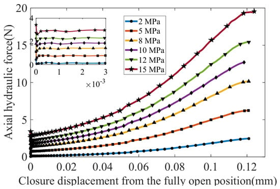
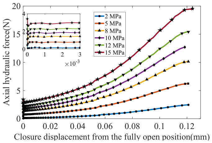
After the electromagnetic actuator is de-energized, the valve core moves toward the valve seat under the combined action of the return-spring force and the hydraulic force. The transient variation in the hydraulic force during this process is shown in Figure 7.

Figure 7. Variation in the axial hydraulic force with valve core displacement during closure under different pressure differentials.

During the initial stage of closure, the axial hydraulic force decreases to approximately 0.4–0.8 N as the flow field adjusts to the changing flow passage, while remaining directed toward the valve seat. With further valve core displacement, the flow velocity around the spherical head increases and the local pressure distribution changes, causing the hydraulic force to recover and then increase progressively. The increase becomes more pronounced when the displacement exceeds approximately 0.01 mm from the fully open position.

These results show that the transient hydraulic force is non-monotonic during the initial closure stage and cannot be represented adequately by a constant load. Throughout the analyzed process, it acts in the closing direction and therefore assists the return spring in closing the valve core.

6. Simulation and Experimental Testing

6.1. System-Level Pressure Unloading Simulation

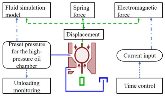
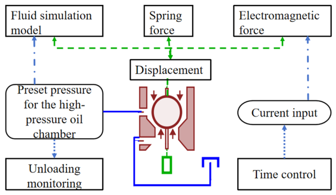
A coupled Simulink–AMESim model was used to evaluate the system-level pressure unloading response, as shown in Figure 8. The model represents the oil chamber, unloading valve, moving valve core, return spring, and displacement constraint, while the electromagnetic and hydraulic-force characteristics obtained from the preceding analyses are incorporated into the valve dynamic model.

Figure 8. Simulink-AMESim simulation framework for system-level pressure unloading.

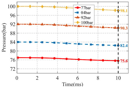
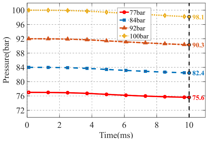
Four initial pressure conditions of 100, 92, 84, and 77 bar were considered, corresponding to the operating pressure range investigated in the injector test system. The pressure unloading process was simulated over a 10 ms unloading window. The simulated pressure responses under the four initial pressure conditions are shown in Figure 9.

Figure 9. Simulation results for pressure unloading under different initial pressure conditions.

As shown in Figure 9, the pressure in the oil chamber decreases after the unloading valve is actuated. For the initial pressures of 100, 92, 84, and 77 bar, the simulated pressures decrease to 98.1, 90.3, 82.4, and 75.6 bar, respectively, at the end of the 10 ms unloading window. The corresponding pressure drops are 1.90, 1.70, 1.60, and 1.40 bar, respectively. The relative pressure drops calculated from the simulated initial pressures are 1.90%, 1.85%, 1.90%, and 1.82%, respectively.

It should be noted that the 10 ms system-level simulation is different from the 1 ms local transient CFD analysis presented in Section 5. The 1 ms CFD calculation was used to resolve the transient variation in the hydraulic force during valve core closure, whereas the 10 ms Simulink–AMESim simulation was used to evaluate the resulting pressure unloading response of the integrated hydraulic system. Therefore, the two simulation time scales correspond to different modeling objectives.

The simulated initial and final pressures, together with the corresponding experimental results, are summarized in Table 5 for quantitative comparison.

Table 5. Comparison of simulated and experimental pressure unloading characteristics.

Initial Pressure (bar)		Final Pressure (bar)		Pressure Drop (bar)		Relative Pressure Drop (%)
Simulation	Experiment	Simulation	Experiment	Simulation	Experiment	Simulation	Experiment
100	100.5	98.1	98.5	1.9	2	1.9	1.99
92	91.9	90.3	90	1.7	1.9	1.85	2.07
84	84.2	82.4	82.8	1.6	1.4	1.9	1.66
77	77.13	75.6	75.77	1.4	1.36	1.82	1.76

6.2. Experimental Validation of Pressure Unloading Performance

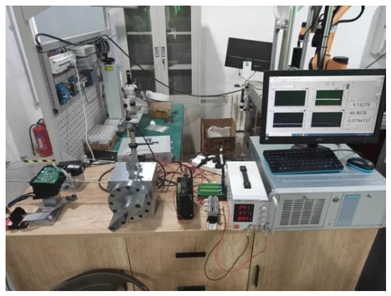
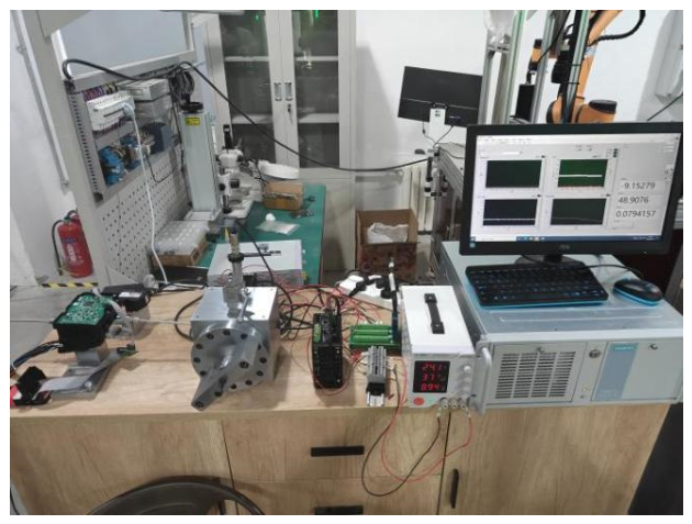
A pressure unloading test bench was constructed to experimentally evaluate the system-level pressure unloading performance of the developed valve in the integrated back pressure assembly, as shown in Figure 10. Four tests were conducted under initial pressures representative of the operating pressure range of the injector test system. No. 0 diesel was used as the working fluid at ambient temperature.

Figure 10. Pressure unloading test bench.

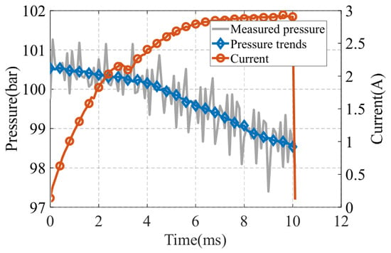
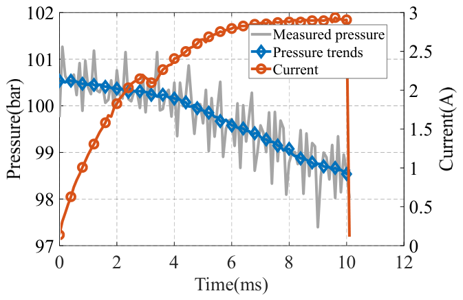
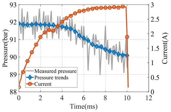
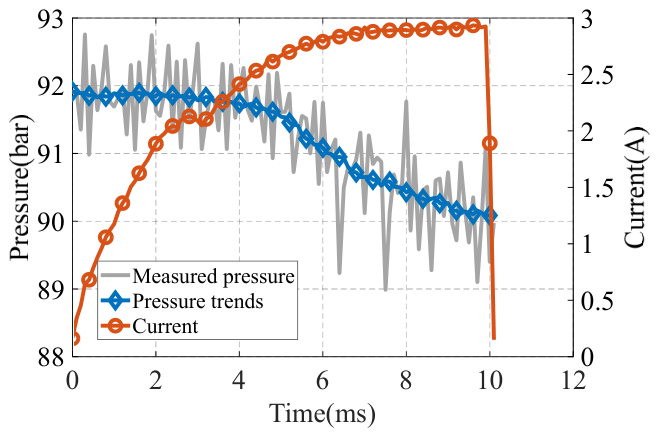
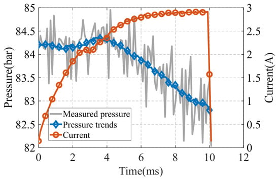
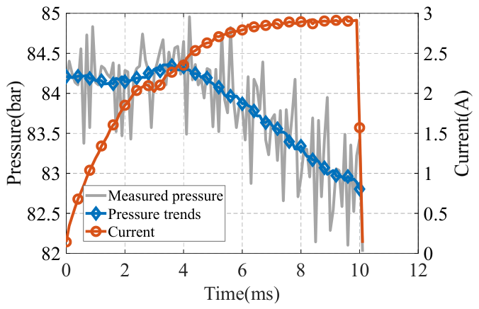
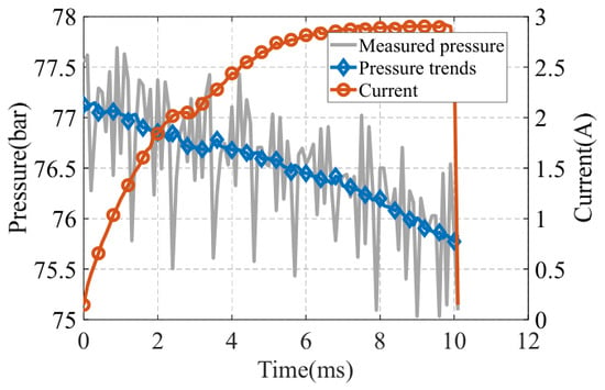
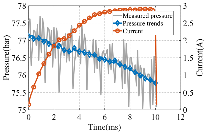
The measured pressure signals exhibit fluctuations during the unloading process, as shown in Figure 11, Figure 12, Figure 13 and Figure 14. To extract the overall pressure unloading trend from the fluctuating signals, a moving-average smoothing method was applied using the movmean function in MATLAB (Version: R2017b), with a window size equal to one-fifth of the total number of sampled points and a minimum of five points.

Figure 11. Experimental pressure response at an initial pressure of 100.5 bar.

Figure 12. Experimental pressure response at an initial pressure of 91.9 bar.

Figure 13. Experimental pressure response at an initial pressure of 84.2 bar.

Figure 14. Experimental pressure response at an initial pressure of 77.13 bar.

Because the raw pressure signals contain fluctuations, the instantaneous maximum and minimum values were not used for quantitative evaluation. Instead, the initial and final pressures were extracted from the moving-average-smoothed trends over the same 10 ms window.

Based on the moving-average-smoothed pressure trends shown in Figure 11, Figure 12, Figure 13 and Figure 14, the initial pressures were 100.50, 91.90, 84.20, and 77.13 bar, while the corresponding pressures at 10 ms were 98.50, 90.00, 82.80, and 75.77 bar, respectively. The resulting pressure drops were therefore 2.00, 1.90, 1.40, and 1.36 bar. The corresponding relative pressure drops were 1.99%, 2.07%, 1.66%, and 1.76%, respectively.

6.3. Comparison Between Simulation and Experiment

The simulated and experimental pressure unloading characteristics are compared in Table 5. To ensure consistency between the numerical and experimental evaluations, the pressure change in both cases was determined over the same 10 ms unloading window. For the experimental tests, the initial and final pressures were obtained from the moving-average-smoothed pressure trends shown in Figure 11, Figure 12, Figure 13 and Figure 14 rather than from the instantaneous fluctuations of the raw pressure signals.

As shown in Table 5, the simulated pressure drops ranged from 1.40 to 1.90 bar, compared with 1.36–2.00 bar in the experiments. The absolute differences between the simulated and experimental pressure drops were 0.04–0.20 bar and showed no monotonic dependence on the initial pressure. The corresponding relative pressure drops were 1.82–1.90% in simulation and 1.66–2.07% in the experiments. The experimental results therefore provide system-level experimental evidence of the pressure unloading behavior predicted by the coupled simulation under the investigated operating conditions.

7. Conclusions

(1)

A high-speed unloading valve was developed for the back pressure assembly of an injector test system, and an electromagnetic–mechanical–fluid coupled model was established to describe its operating characteristics. The valve was investigated with particular emphasis on rapid pressure unloading.

(2)

Steady-state CFD underpredicted the experimental flow rates by approximately 18.1–20.4%. Quantitative sensitivity analysis showed that the combined dimensional tolerances, mesh resolution, turbulence model selection, and measurement uncertainty could not fully explain the discrepancy. Therefore, no arbitrary error allocation or specific causal attribution was introduced for the remaining difference.

(3)

Three-dimensional CFD revealed both axial and radial hydraulic forces caused by the asymmetric flow field. The axial forces predicted by the 2D and 3D models differed by 1.69–4.26%, supporting the use of the 2D model for transient axial-force analysis. During valve closure, the axial hydraulic force exhibited an initial decrease followed by recovery and subsequent increase, indicating that the transient hydraulic force should be considered in the dynamic analysis.

(4)

System-level Simulink–AMESim simulations and experiments showed comparable pressure unloading characteristics within the investigated operating conditions, with pressure reductions of approximately 1.4–2.0 bar in simulation and 1.36–2.00 bar in experiments over 10 ms. The results provide system-level experimental evidence for the pressure unloading function of the proposed valve under the intended application conditions.

References

- Song, J.D. Study on Injection Characteristics Test Method and Law of High Power Marine Injector. Master’s Thesis, Harbin Engineering University, Harbin, China, 2022. [Google Scholar]
- Zhou, Q.Z.; Zhang, Y.Y.; Qi, W.Y. Investigation on the Key Factors Affecting the Accuracy of Fuel Injection Rate Measurement by Zeuch Method. Chin. Intern. Combust. Engine Eng. 2019, 40, 28–35. [Google Scholar]
- Tao, F. A Study on Injection Rate of Common Rail System by the Zeuch Method. Master’s Thesis, Harbin Engineering University, Harbin, China, 2018. [Google Scholar]
- Meng, A.H.; Gao, X.; Li, N.N.; Garris, C. Study on the Effect of Structural Parameters on the Linear Control Performance of High Speed On-Off Valve Based on Flow Field Analysis. In Proceedings of the Brake Colloquium & Exhibition-38th Annual, San Antonio, TX, USA, 11–14 October 2020. [Google Scholar]
- Mu, H.Y.; Cheng, S.; Li, K.; Li, L.; Pan, P.; Zhao, X. Design and Verification of Linear High-speed On-off Valve. J. Mech. Eng. 2021, 57, 247–254. [Google Scholar] [CrossRef] [Scilit]
- Wang, C.G.; Liu, X.W.; Liu, Z.L.; Zhang, J. Research on Factors that Affect Hydraulic Pressure of High Speed On-Off Valve. Mach. Tool Hydraul. 2018, 46, 50–54. [Google Scholar]
- Liu, H.C.; Wu, J.J.; Zhou, T.F.; Li, L. Flow field analysis and structure optimization of throttling area in electromagnetic high-speed on-off valve. Chin. Hydraul. Pneum. 2025, 49, 107–115. [Google Scholar]
- Xu, B.; Ding, R.; Zhang, J.; Su, Q. Modeling and Dynamic Characteristics Analysis on a Three-stage Fast-response and Large-flow Directional Valve. Energy Convers. Manag. 2014, 79, 187–199. [Google Scholar] [CrossRef] [Scilit]
- Li, S.; Wu, P.; Cao, L.; Wu, D.; She, Y. CFD Simulation of Dynamic Characteristics of a Solenoid Valve for Exhaust Gas Turbocharger System. Appl. Therm. Eng. 2017, 110, 213–222. [Google Scholar] [CrossRef] [Scilit]
- Manring, N.D.; Zhang, S. Pressure Transient Flow Forces for Hydraulic Spool Valves. J. Dyn. Syst. Meas. Control 2012, 134, 034501. [Google Scholar] [CrossRef] [Scilit]
- Lisowski, E.; Czyżycki, W.; Rajda, J. Three-dimensional CFD Analysis and Experimental Test of Flow Force Acting on the Spool of Solenoid Operated Directional Control Valve. Energy Convers. Manag. 2013, 70, 220–229. [Google Scholar] [CrossRef] [Scilit]
- Li, R.C.; Wang, Z.B.; Xu, J.K.; Yuan, W.T.; Wang, D.W.; Ji, H.L.; Chen, S. Design and optimization of hydraulic slide valve spool structure based on steady state flow force. Flow Meas. Instrum. 2024, 96, 102568. [Google Scholar] [CrossRef] [Scilit]
- Sang, Y.; Wang, X.; Sun, W. The Dynamic Characteristics of a Small Hydraulic Poppet Safety Relief Valve. Int. J. Fluid Mach. Syst. 2020, 13, 233–240. [Google Scholar] [CrossRef] [Scilit]
- Min, W.; Wang, H.; Zheng, Z.; Wang, D.; Ji, H.; Wang, Y. Visual Experimental Investigation on the Stability of Pressure Regulating Poppet Valve. Proc. Inst. Mech. Eng. Part C J. Mech. Eng. Sci. 2020, 234, 2329–2348. [Google Scholar] [CrossRef] [Scilit]
- Zhao, J.H.; Zhao, S.; Grekhov, L. Study on Transient Fuel Hydrodynamic Force Characteristics of High-speed Solenoid Valve for Common Rail Injector. Int. J. Automot. Technol. 2020, 21, 1257–1269. [Google Scholar] [CrossRef] [Scilit]
Disclaimer/Publisher’s Note: The statements, opinions and data contained in all publications are solely those of the individual author(s) and contributor(s) and not of MDPI and/or the editor(s). MDPI and/or the editor(s) disclaim responsibility for any injury to people or property resulting from any ideas, methods, instructions or products referred to in the content. |
© 2026 by the authors. Licensee MDPI, Basel, Switzerland. This article is an open access article distributed under the terms and conditions of the Creative Commons Attribution (CC BY) license.