


Abstract
To address the small ATC-63 record set for collapse-oriented motion selection and the limited interpretability of data-driven approaches, this study proposes a framework for identifying structural-collapse-critical ground motions. Using 5074 records from the PEER NGA-West2 database, we applied STA/LTA event detection and extracted multi-source features. A Gaussian mixture model (GMM) was then used to perform unsupervised clustering and identify four physically interpretable groups. LightGBM, XGBoost, and Random Forest were employed to test the separability of the cluster labels, with all three models achieving F1 scores above 0.89 and LightGBM reaching an accuracy of about 93%. SHAP-based feature-importance analysis was used at the model level to clarify feature contributions and improve interpretability. Cluster 2 exhibits markedly higher relative seismic energy, stronger time-domain variability, and more dominant frequencies, forming a typical strong-motion hazard signature. For external engineering verification, 22 ATC-63 far-field records were mapped onto the full dataset to examine cluster-level enrichment and coverage. Cluster 2 shows significant enrichment in engineering markers and high coverage and is therefore identified as the collapse-sensitive phenotype cluster (COP). Overall, the framework provides a technical basis for ground-motion selection in collapse assessment, fragility analysis, and design evaluation.
1. Introduction
Collapse assessment quantifies the near-collapse nonlinear response and failure probability of structures, and underpins safety-margin calibration and ground-motion selection in performance-based seismic design [1]. The methodology has evolved from incremental dynamic analysis (IDA) to multi-stripe and cloud approaches for probabilistic fragility and collapse evaluation, with Bayesian updating and GP/ML surrogate models further improving efficiency and robustness [2]. Regardless of the specific analysis procedure, the statistical representativeness, traceability, and intensity scaling of the input ground motions remain key factors controlling the credibility of the collapse assessment [3]. Different ground-motion sets can produce markedly different fragility curves and safety-margin estimates, so a sufficiently representative and properly scaled record set is essential for reliable, robust, and reproducible collapse-resistant design.
In current collapse assessment practice, the ATC-63 (FEMA P-695) [4] recommended ground-motion set is commonly used as the benchmark input for incremental dynamic analysis (IDA) [2], owing to its high level of standardization and strong cross-study comparability. However, its sample size is limited (22 far-field records for typical building systems), which can amplify sampling uncertainty in fragility fitting and collapse margin ratio (CMR) estimation and increase sensitivity to a small number of records and scaling rules [5]. Moreover, insufficient coverage of key characteristics—such as spectral shape, duration, and near-fault pulse effects—may constrain the transferability of conclusions across different hazard scenarios [6,7]. Therefore, while preserving the advantages of standardization and comparability, it is necessary to develop an expanded ground-motion library with stronger statistical representativeness to more reliably support near-collapse assessment. To enhance traceability in record selection and consistency with seismic hazard, researchers have further proposed a range of “spectral-shape-consistent” selection frameworks, such as the Conditional Mean Spectrum (CMS) and the Generalized Conditional Intensity Measure (GCIM) approaches [8,9]. However, these methods primarily impose constraints on spectral shape together with a limited number of intensity-related measures, and may still have insufficient discriminative capability for separating records that—under the same intensity level—lead to markedly different near-collapse responses due to differences in duration, the energy-input process, and nonstationarity.
Many intensity measures (IMs) have been proposed to quantify and rank ground-motion severity, but no single IM can fully capture spectral shape, duration, and energy evolution, nor reliably distinguish records that drive markedly different near-collapse responses [10,11]. Meanwhile, the rapid growth of strong-motion networks has produced massive datasets that mix mainshocks, aftershocks, microtremors, and noise, making manual screening and expert-based classification difficult to scale and standardize [12,13]. In this context, machine learning methods with efficient feature extraction and pattern recognition have become a key route for ground-motion identification and hazard analysis, providing scalable and reproducible support for expanding collapse-oriented record libraries [14,15,16,17]. More broadly, existing studies generally follow two complementary directions: (i) record screening and library expansion, where feature representations and unsupervised clustering are used to identify spectral/waveform families and enable representative sampling; and (ii) computational acceleration for seismic assessment, where surrogate models, active learning, or ensemble learning are adopted to reduce the number of costly nonlinear time–history analyses (NLTHA), thereby speeding up the estimation of probabilistic demand/fragility curves [18,19].
Machine learning applications in seismology and earthquake engineering are mainly based on supervised and unsupervised learning. Supervised learning can yield clearer semantics when labels are available, but it relies on high-quality annotations and often suffers from limited generalization across scenarios [17,20]. By contrast, unsupervised learning can reveal latent structures and patterns in records without labels and has been widely applied to waveform clustering and event identification [21,22,23]. Existing work often combines feature engineering with unsupervised models (e.g., Gaussian Mixture Models (GMMs) and autoencoders) to achieve efficient clustering, and such strategies have been validated in tasks such as weak-event detection and clustering in reduced-dimensional feature spaces [24,25]. These advances provide a methodological basis for extracting waveform/spectral families from large candidate libraries and reducing redundancy. However, a key step for engineering-oriented use remains insufficiently addressed: how to translate unsupervised statistical groupings into screening criteria that are auditable and reproducible—without relying on costly structural-response labels—and how to establish a testable verification chain via external engineering labels.
SHAP (SHapley Additive exPlanations) uses game-theoretic Shapley values to quantify local and global feature importance in tree-based models such as TreeSHAP [26]. Recent studies combine SHAP with unsupervised clustering by training classifiers on cluster labels or using mixture-model responsibilities to derive cluster-level importance maps [27,28]. This allows clustering results to be turned into collapse-oriented, interpretable screening rules that highlight key properties (spectral shape, duration, energy concentration, near-fault pulses) and improve the traceability and engineering acceptability of record inclusion/exclusion decisions.
In conclusion, this study develops a collapse-oriented ground-motion identification framework using 5074 records (M > 6.0) from PEER NGA-West2, integrating four modules: feature representation, unsupervised clustering, explainable ensemble learning, and engineering-label validation. First, clustering is performed in a multi-domain feature space to obtain candidate clusters; then LightGBM, XGBoost, and Random Forest models are trained as supervised surrogates, and SHapley Additive exPlanations (SHAP) is used to derive cluster-level feature profiles; finally, ATC-63 records are introduced to conduct cluster-level coverage and enrichment tests, enabling a verifiable alignment between clustering outcomes and engineering semantics. It should be emphasized that this work does not aim to propose a new collapse surrogate prediction model or to directly fit risk/probability curves; rather, it focuses on a workflow for identifying and expanding collapse-oriented candidate record libraries. The proposed framework provides an interpretable and reusable technical basis for subsequent ground-motion selection, fragility analysis, design-parameter calibration, and post-earthquake assessment.
2. Research Scope and Data Acquisition
The data used in this study were sourced from the NGA-West2 strong ground motion database developed by the Pacific Earthquake Engineering Research Center (PEER). As one of the key outcomes of the Next Generation Attenuation (NGA) project, this database serves as a core data source for the development of various internationally recognized ground-motion prediction equations (GMPEs). It has been widely used in the formulation of seismic design codes and assessment guidelines by authoritative organizations such as FEMA and ATC, including ATC-63 and FEMA P-695. NGA-West2 also provides traceable event- and station-level metadata (including latitude and longitude), so the spatial locations of the records used in this study can be directly verified by querying the database. In addition, event magnitude in NGA-West2 is reported using the moment magnitude scale, Mw (moment magnitude); throughout this paper, the magnitude M refers to Mw.
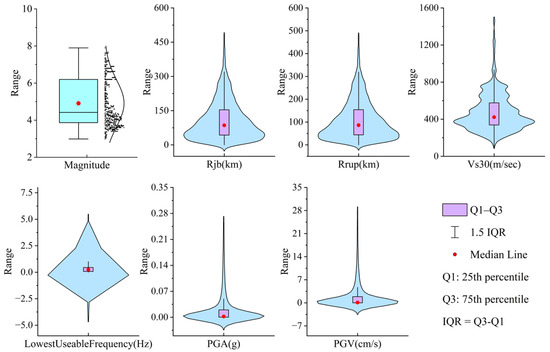
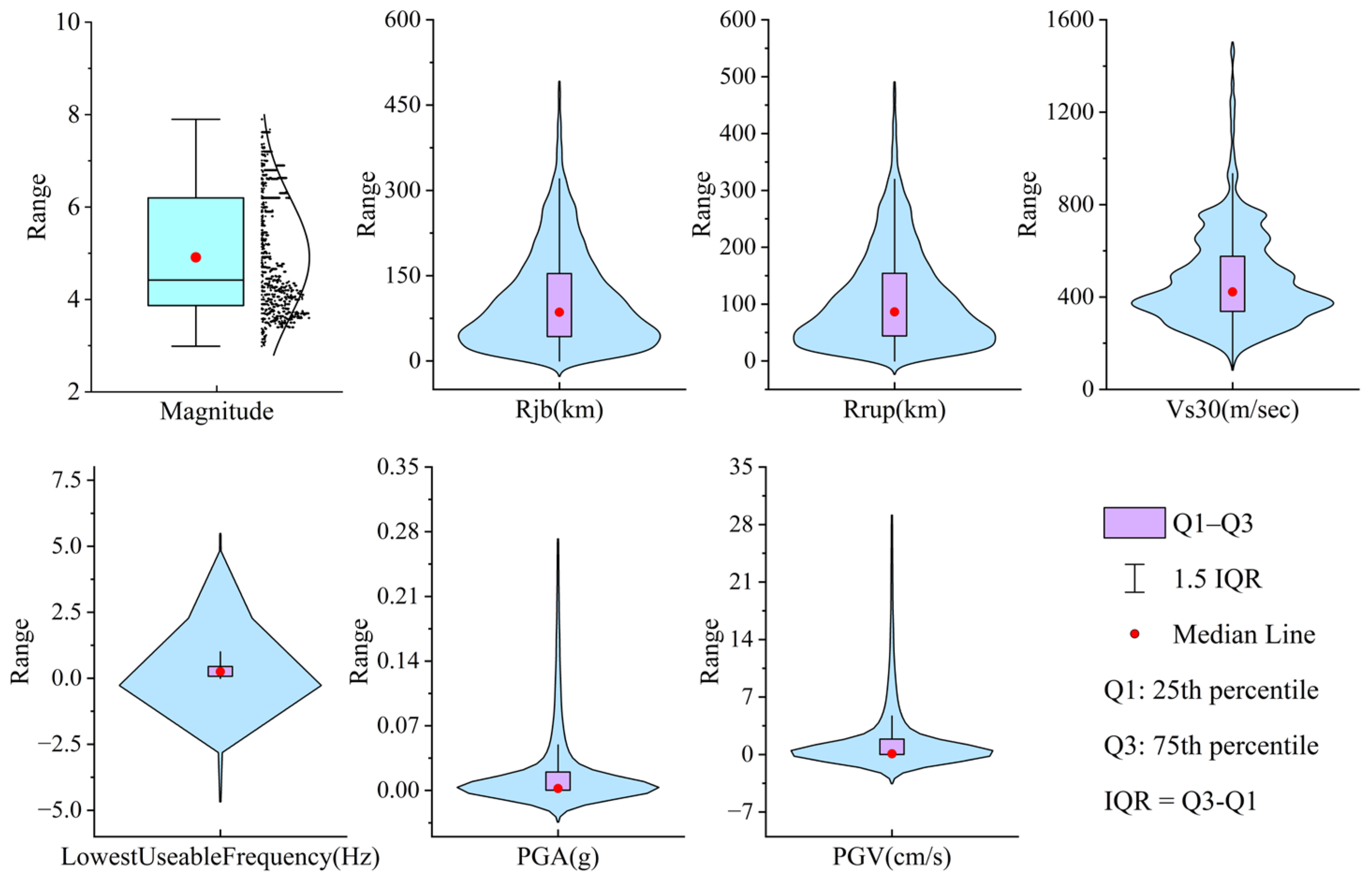
This study compiled 21,336 three-component acceleration time histories from the database, covering most major shallow earthquakes since 1935 with magnitudes from M 3.0 to 7.9. The distance coverage is wide, including very near-distance records (for which the fault distance and/or epicentral distance can be close to 1 km in some cases) as well as far-distance records (with maximum distances exceeding 1000 km). Meanwhile, the site conditions span from soft soil to hard rock, with Vs30 values ranging from 94 to 2100 m/s (Figure 1), indicating good diversity in ground-motion intensity and site representativeness.
Figure 1.
Statistical characteristics of the 21,336 ground motion records.
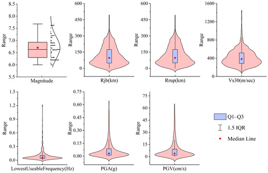
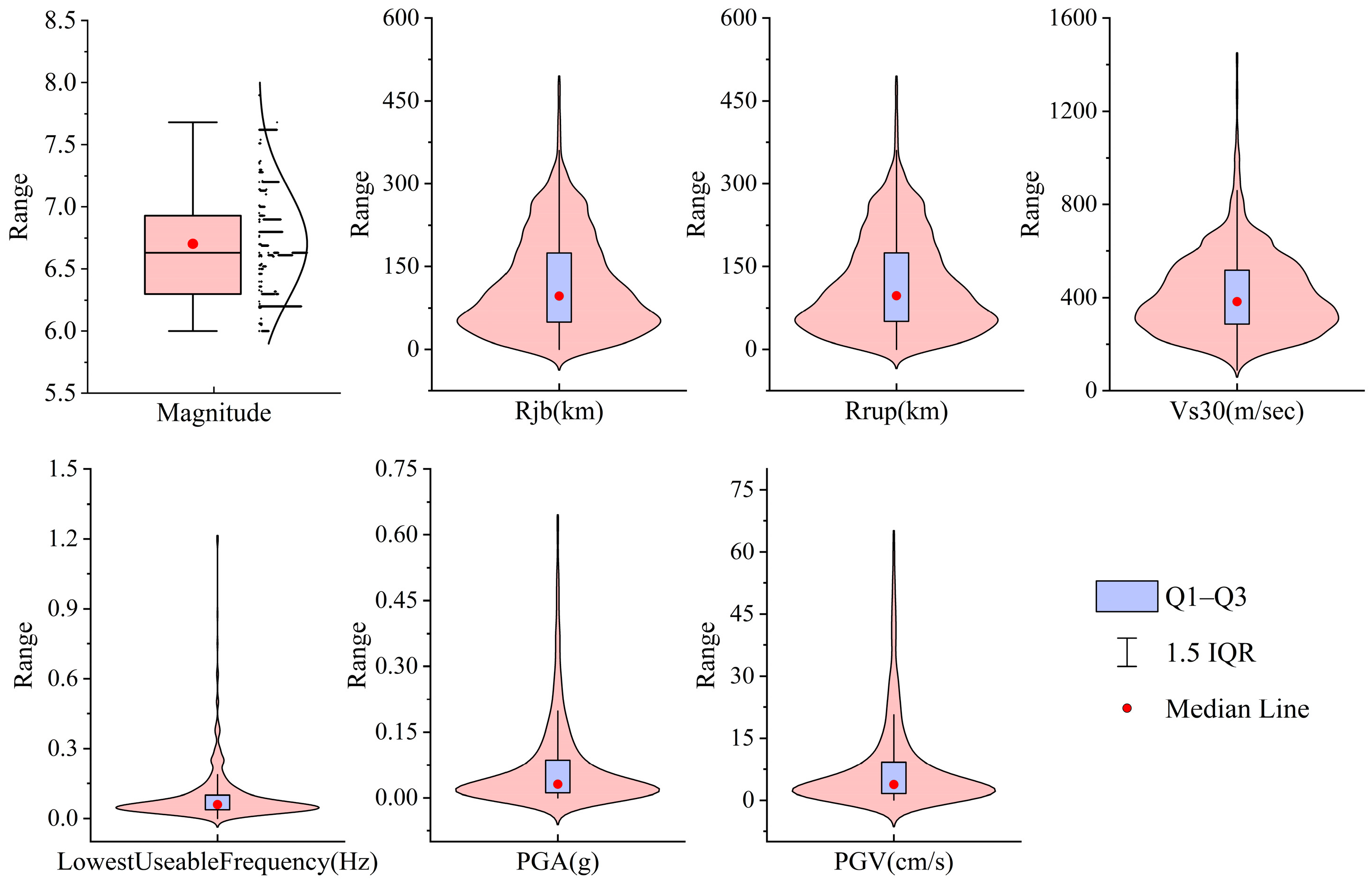
To ensure sufficient engineering relevance and damage potential, this study followed the requirements on representative input motions in international seismic design codes (e.g., ASCE 7 [29], Eurocode 8 [30]) and ATC-63 [4] recommendations, and removed low-magnitude records unlikely to cause significant damage. In total, 5074 records with M > 6.0 were retained as the core dataset and candidate pool for unsupervised clustering, with their intensity statistics as shown in Figure 2.
Figure 2.
Statistical characteristics of the 5074 ground-motion records with M > 6.0.
3. Framework for Structural-Collapse-Sensitive Ground-Motion Identification
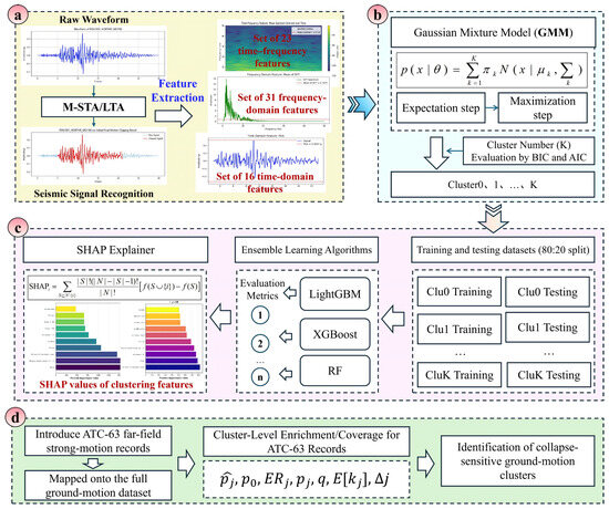
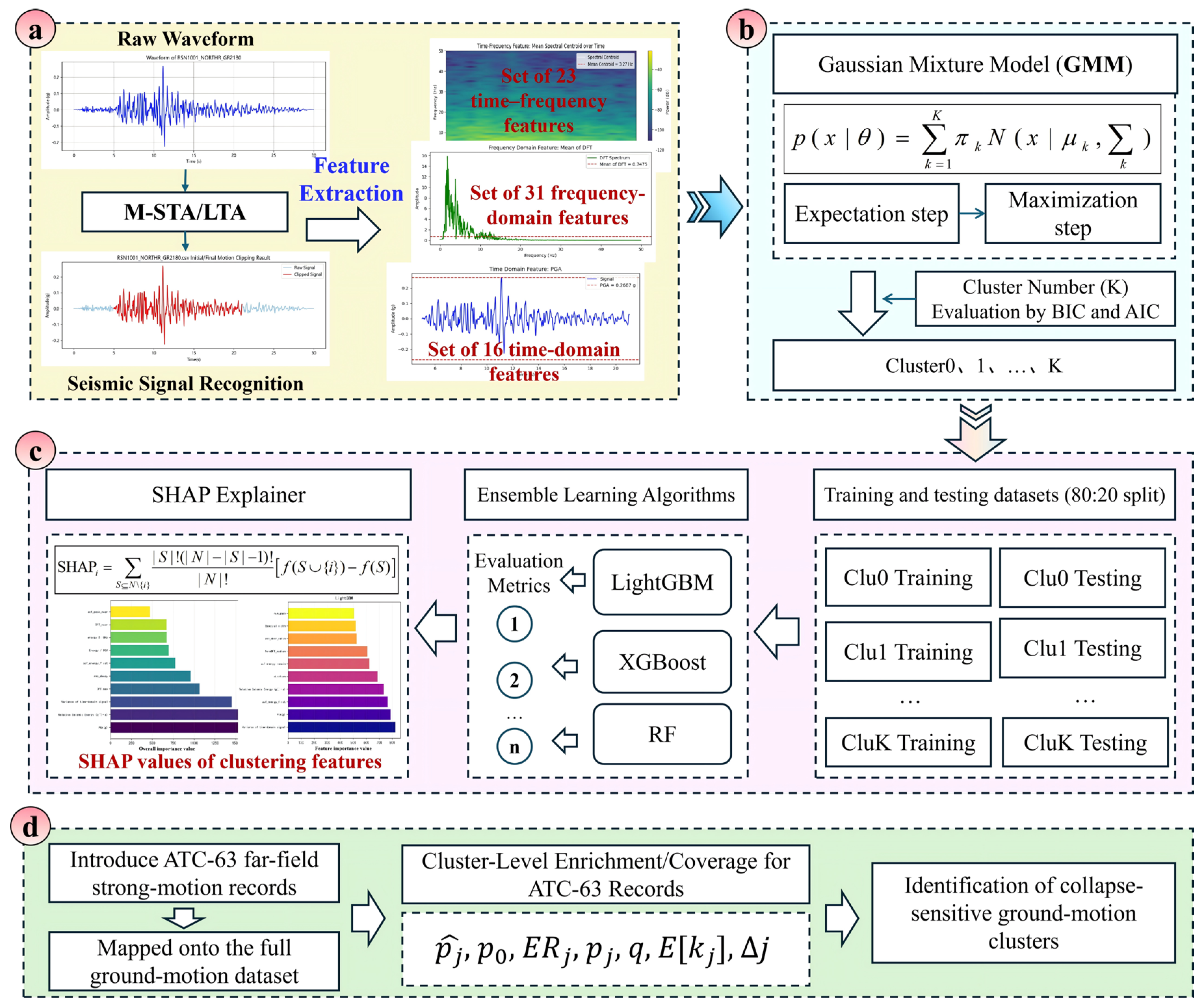
The collapse-sensitive ground-motion identification framework developed in this study, based on unsupervised clustering and explainable ensemble learning, is shown in Figure 3. It consists of four stages:
Figure 3.
A framework for structural-collapse-sensitive ground-motion identification. (a) Preprocessing and feature extraction of seismic signals. (b) Unsupervised clustering of seismic waveforms. (c) Interpretability analysis of the clustering results. (d) Identification of ground motions sensitive to structural collapse.
- (1)
- Detection of potential earthquake signals and feature extraction using the STA/LTA (short-term average/long-term average) window method;
- (2)
- Unsupervised clustering of the preprocessed signals using a Gaussian mixture model (GMM);
- (3)
- Interpretation of the clustering results and their discrimination mechanisms with ensemble-learning algorithms and SHAP;
- (4)
- Introduction of ATC-63 far-field ground motions to perform cluster-level enrichment and coverage tests and to identify the collapse-sensitive ground-motion cluster.
3.1. Detection of Potential Seismic Signals
In seismic signal processing, accurately identifying the onset and termination of seismic events is critical for subsequent feature extraction and pattern analysis. As seismic signals are often obscured by environmental noise, robust detection algorithms are required to identify potential shaking segments within continuous time series. The STA/LTA (Short-Time Average/Long-Time Average) window detection method is a classic and efficient technique for seismic event detection. Its fundamental principle is to determine the occurrence of an event by comparing the average signal energy within a short-time window to that within a long-time window [31]. When the short-time average (STA) of the signal significantly exceeds the long-time average (LTA), it indicates the possible presence of a transient shaking event, thereby triggering the event onset. Conversely, when the STA falls below the LTA, the signal is considered to have returned to a steady state. The calculation is expressed as follows:
Here, Nsta and Nlta represent the lengths of the short-time and long-time windows, respectively, and x(i) denotes the amplitude of the signal at time point i. When the ratio STA(t)/LTA(t) exceeds a predefined threshold, a seismic event is considered to have occurred. The traditional STA/LTA method offers advantages such as computational simplicity and strong real-time performance. However, it is also sensitive to noise and abrupt fluctuations, which can lead to false detections or missed detections during the initial onset identification of actual seismic events.
To improve the accuracy of detecting the onset of seismic signals and to reduce false or missed detections of seismic events, this study adopts a multi-window Short-Time Average/Long-Time Average (m-STA/LTA) method for seismic signal identification [32]. This method enhances onset detection accuracy by aggregating STA and LTA calculations across multiple time windows, thereby integrating signal characteristics over different temporal scales. Specifically, multiple time window pairs (e.g., 0.5 s and 5 s, 1 s and 10 s) are used to compute STA and LTA values independently, and trigger detection is performed across all window combinations. By aggregating the trigger results from multiple window pairs, the method effectively reduces noise interference and enhances both the accuracy and robustness of seismic event detection.
3.2. Feature Extraction of Seismic Signals
Before performing unsupervised clustering, it is necessary to compute various types of features to comprehensively characterize the properties of seismic signals. Following the method proposed by Provost et al. [33], this study extracts 70 features from 5074 ground motion records, which are categorized into time-domain, frequency-domain, time–frequency, and signal quality groups. Detailed definitions and formulas for these features are provided in Appendix A (Table A1, Table A2, Table A3 and Table A4). It should be emphasized that the multi-domain features are used to construct a structured characterization of waveform morphology–energy–duration process–spectral structure–signal integrity, rather than to treat multiple correlated intensity-related indicators in parallel as engineering criteria.
In addition, this study does not include response-spectrum-type indicators such as Sa(T, ξ) and Sd(T, ξ) as clustering input features, because their values depend on assumptions about the structural period and damping ratio. This dependence may readily turn the clustering outcome into a “structure-specific period grouping,” which is not conducive to forming a waveform-phenotype partition that can be reproduced using the time histories alone. In the near-collapse regime, response divergence is influenced not only by spectral amplitude but also by duration, the energy-input process, and frequency-band coverage. Therefore, we adopt multi-domain waveform features to provide a structured representation of this information.
3.3. Gaussian Mixture Model (GMM)
Unsupervised learning methods are widely applied in the classification and pattern recognition of seismic signals, particularly after signal processing and feature extraction. The Gaussian Mixture Model (GMM) is a commonly used unsupervised clustering method that models and partitions seismic signal features in a probabilistic framework [24,34]. Specifically, GMM assumes that the data are generated from a mixture of multiple Gaussian (normal) distributions, where each data point is associated with one of these components. Each Gaussian component is characterized by its own mean, variance, and mixing weight. By applying GMM to cluster seismic signals, the model is trained using the Expectation-Maximization (EM) algorithm to categorize different types of seismic events. The probability density function of the model is expressed as:
Here, πk denotes the weight of the k-th Gaussian component, and uk and ∑k represent the mean vector and covariance matrix of the k-th Gaussian component, respectively. N(x|uk, ∑k) is the probability density function of the Gaussian distribution, and the EM algorithm iteratively estimates these parameters through optimization.
However, a key challenge in applying GMM for unsupervised clustering is determining the optimal number of clusters K. An excessively small number of clusters may lead to underfitting, while an excessively large number may result in overfitting. To address this issue, the study adopts two commonly used model selection criteria: the Akaike Information Criterion (AIC) [35] and the Bayesian Information Criterion (BIC) [36,37], which evaluate the trade-off between model goodness-of-fit and complexity across a range of candidate cluster numbers. The evaluation expressions for AIC and BIC are given as follows:
Here, L denotes the maximum likelihood estimate of the model, k is the number of free parameters, and NNN represents the total number of samples. Both AIC and BIC are evaluation criteria designed to balance model fitting accuracy and complexity. BIC imposes a stricter penalty on model complexity compared to AIC and, therefore, tends to favor more parsimonious models when the sample size is large, helping to mitigate the risk of overfitting.
By integrating GMM with model selection criteria such as AIC and BIC, the potential distribution structure of seismic signals can be adaptively modeled, thereby avoiding or reducing the uncertainty associated with subjectively specifying the number of clusters.
3.4. Interpretability of Clustering Results
3.4.1. Ensemble Learning Algorithms
To further investigate the discriminative power of individual seismic features across different clusters, this study employs tree-based ensemble learning methods, including LightGBM (Light Gradient Boosting Machine) [38], Random Forest (RF) [39], and XGBoost (Extreme Gradient Boosting) [40]. Compared to individual models, ensemble methods combine multiple weak learners to enhance overall performance. They are particularly well-suited for handling the complex characteristics commonly observed in seismic signals, such as multi-source heterogeneity, uneven feature distributions, and strong local fluctuations. In addition, the aforementioned models possess strong nonlinear modeling capabilities, are robust to noise, exhibit low sensitivity to high-dimensional features, and do not require explicit modeling of feature interdependencies. They are capable of automatically identifying key variables that have a significant impact on classification outcomes. Therefore, these methods are employed in this study to evaluate the discriminative contribution and interpretive value of the extracted seismic signal features with respect to the unsupervised clustering results.
Given that the GMM-based unsupervised clustering process has already assigned a cluster label to each seismic signal, the study uses all extracted features as input variables and the GMM-derived cluster labels as the target variable. The dataset is split into training and testing subsets in an 80:20 ratio for model training.
To better accommodate the feature distribution of seismic signals and enhance model performance, this study employs a grid search strategy to explore a predefined hyperparameter space and identify the optimal combination for achieving the best results. For LightGBM and XGBoost, the tuned hyperparameters include the number of trees (n_estimators), maximum tree depth (max_depth), learning rate (learning_rate), subsample ratio (subsample), and feature sampling ratio (colsample_bytree). For Random Forest, the tuned hyperparameters include the maximum number of features considered for splitting (max_features), the minimum number of samples required to split an internal node (min_sample_split), and the minimum number of samples required to be at a leaf node (min_sample_leaf), among others (see Table 1).
Table 1.
Grid search parameter optimization table for LightGBM, XGBoost, and Random Forest (RF).
3.4.2. SHAP-Based Model Explainer
In the machine learning modeling process, interpretability is a key factor in ensuring the credibility and acceptability of the model. To uncover the specific roles of individual seismic signal features in the model’s decision-making process, this study introduces SHAP-based interpretability analysis. This study introduces SHAP (SHapley Additive exPlanations) [41,42] as an interpretability tool to quantitatively analyze the contribution of each feature to the predictions made by the ensemble models. SHAP is a model interpretability method derived from game theory, which fairly allocates the marginal contribution of each feature to the model output. This enables both global and local explanations of model prediction results. As a powerful model interpretability tool, SHAP assigns a value to each extracted seismic signal feature, representing its contribution to the model’s prediction.
Specifically, the SHAP value quantifies the average marginal contribution of a given feature to the prediction output across all possible subsets of features. The calculation is given by the following formula:
Here, SHAPi denotes the SHAP value of feature i, N represents the full set of features, S is any subset of features that does not include feature i, and f(S)denotes the model’s prediction output based on the feature subset S. A positive SHAP value indicates that the feature has a positive (supporting) influence on the prediction for the current sample, while a negative SHAP value suggests that the feature has a suppressing effect on the prediction outcome. Moreover, the larger the absolute value of a SHAP score, the more significant the feature’s influence on the model’s decision.
By incorporating the SHAP method, this study enables visual interpretation and ranking analysis of seismic signal features in the prediction of each cluster. This facilitates a deeper understanding of the physical significance and distinguishing mechanisms underlying different signal patterns.
3.5. Identification of Collapse-Sensitive Ground Motions
To assess the engineering applicability of the proposed unsupervised clustering and explainable ensemble-learning framework for collapse assessment, this section uses the 22 ATC-63 far-field strong-motion records as external engineering labels. This set has long been used in collapse fragility and capacity studies, with clearly defined selection and scaling criteria, and thus provides a high-hazard reference closely related to collapse. The distribution of ATC-63 records across clusters is evaluated, their within-cluster proportions are compared with those of the full database, and enrichment and coverage tests are carried out. This allows us to examine how well the clustered ground motions align with collapse-related labels and to derive a quantitative basis for expanding collapse-oriented record libraries.
Using the same preprocessing and 70-feature scheme as for the full database, the ATC-63 records are mapped into the full sample space, and their cluster-wise distribution is computed. For each cluster, the within-cluster proportion is compared with the baseline proportion p0 of the full database, and the enrichment ratio ERj and upper-tail hypergeometric probability pj are calculated to test for significant enrichment. FDR-adjusted q-values are used to control multiple testing, and the expected count E[kj] and its deviation Δj are reported to characterize the magnitude and robustness of the enrichment effect.
where pj is the proportion of ATC-63 far-field records in cluster j, with nj the total records in the cluster, and kj the ATC-63 records in that cluster. p0 is the baseline proportion for the full database, where N = 5074 is the total number of clustered records and K = 22 is the total number of ATC-63 far-field records.
4. Results and Discussion of the Proposed Framework
4.1. Unsupervised Clustering of Seismic Waveforms
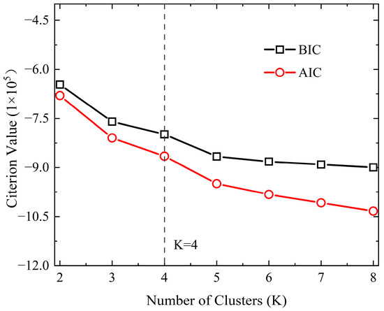
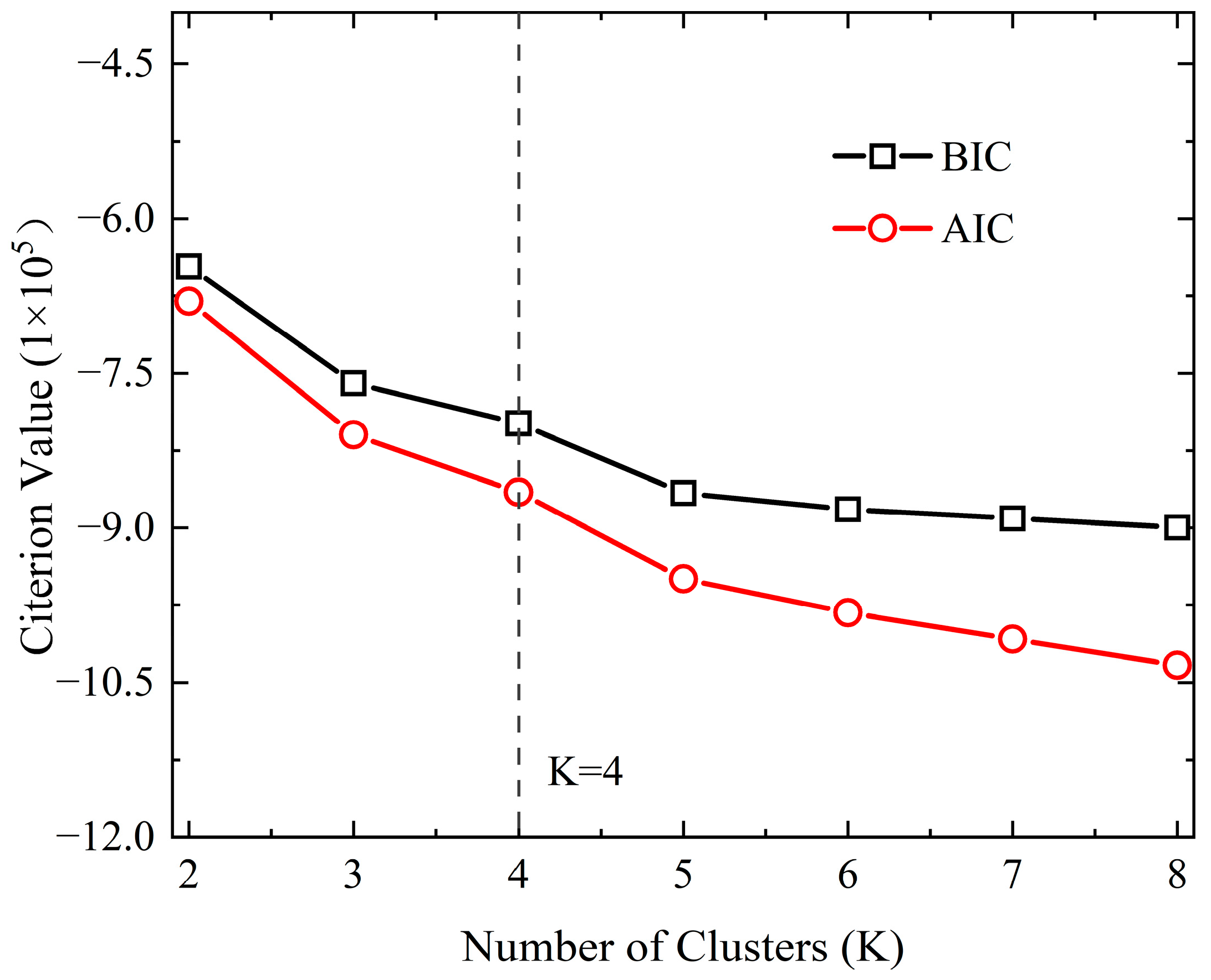
To determine the appropriate number of clusters, this study employs the commonly used Bayesian Information Criterion (BIC) and Akaike Information Criterion (AIC) for evaluation. As shown in Figure 4, both BIC and AIC generally decrease with increasing cluster number K, and their trends are consistent, indicating agreement in their evaluation of the clustering structure. It is worth noting that the curves show a pronounced slowdown in their rate of decline after K = 4, indicating that the marginal improvement in model fit decreases as the number of clusters increases. Since lower BIC and AIC values indicate a better model, the results in the figure suggest that K = 4~8 are all reasonable choices. However, while a larger number of clusters may yield finer classifications, it can also lead to increased analytical complexity. To balance model simplicity and clustering quality, this study ultimately selects K = 4 as the number of clusters for subsequent analysis.
Figure 4.
Variation of the Bayesian Information Criterion (BIC) and Akaike Information Criterion (AIC) with the Number of Clusters in Gaussian Mixture Models (GMM).
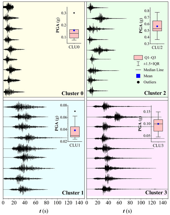
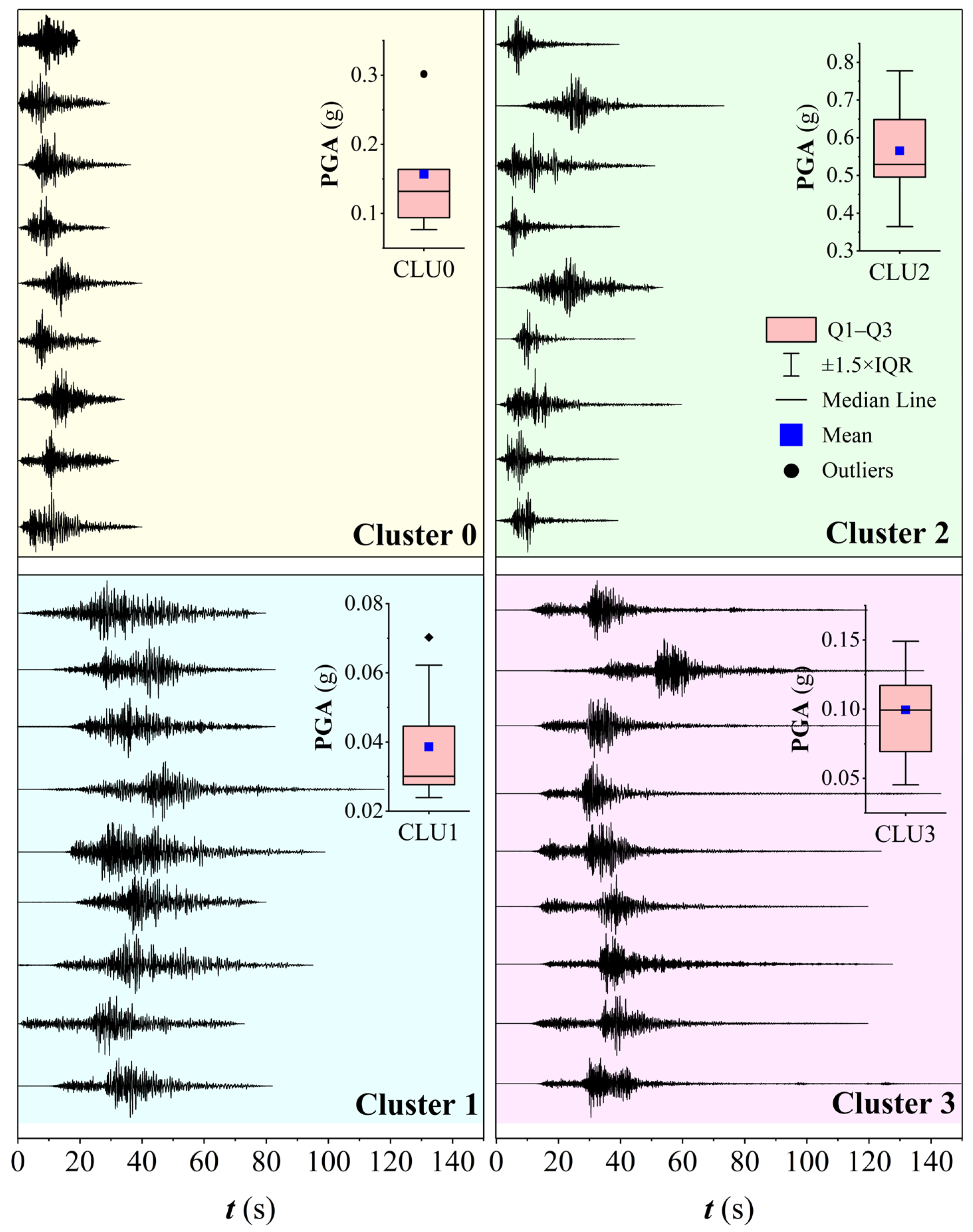
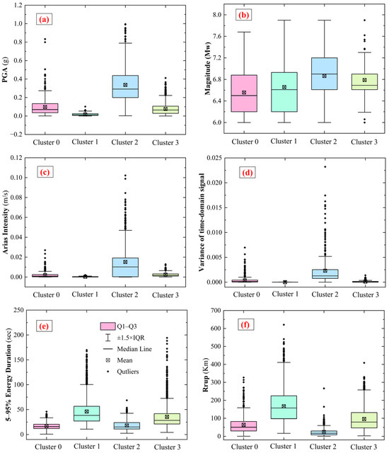
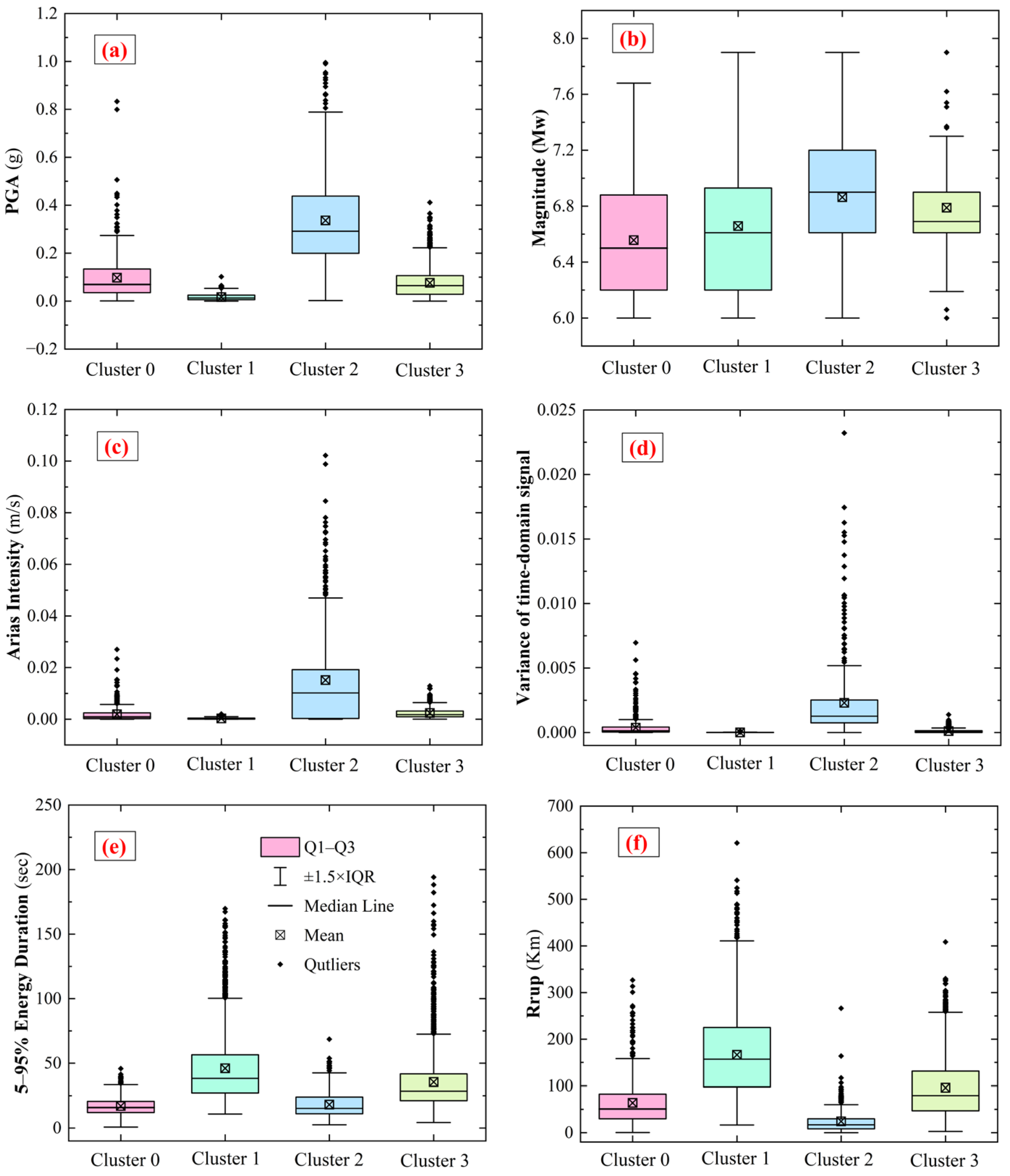
After determining the number of clusters as K = 4, the Gaussian Mixture Model (GMM) is employed to perform unsupervised clustering. To preliminarily identify the differences in ground motion characteristics across clusters, nine normalized acceleration time histories closest to the centroid of each cluster were plotted (Figure 5). In addition, box plots of features extracted from multiple dimensions—including amplitude intensity, energy distribution, duration, waveform volatility, and epicentral distance—were generated (Figure 6) to facilitate a systematic comparative analysis.
Figure 5.
Normalized waveform features of the nine samples closest to each cluster centroid identified by GMM.
Figure 6.
Boxplots of seismic parameters for different clusters identified by unsupervised clustering. (a) PGA; (b) Magnitude; (c) Arias Intensity; (d) Variance of time-domain signal; (e) 5–95% Energy Duration; (f) Rrup.
By comparing the waveform shapes and statistics of the four clusters (Figure 5 and Figure 6), Cluster 0 is characterized by compact records with rapid decay after the peak, short 5–95% significant duration, median-level PGA and Arias intensity, and moderate epicentral distances, representing moderate-intensity, short-duration motions with limited engineering impact. Cluster 1 shows the smallest amplitude fluctuations, low and elongated envelopes with long tails, generally low PGA and Arias intensity, the largest epicentral distances, and relatively long duration, reflecting far-field, low-energy, long-tail motions with relatively low risk. Cluster 2 exhibits a pronounced main energy burst with high and sustained peaks, strong energy concentration, high PGA, Arias intensity, time-domain variance and duration, and smaller epicentral distances, corresponding to near-field or high-energy motions with high damage potential. Cluster 3 shows multi-stage energy release with identifiable gaps between peaks, intermediate amplitude and energy measures, and moderate epicentral distances, representing motions with multiple moderate shocks and intermediate hazard.
In summary, Cluster 2 shows marked extremity across multiple dimensions—including amplitude intensity, energy metrics, duration, waveform volatility, and epicentral distance—making it the most potentially hazardous group of seismic signals among the four clusters.
4.2. Analysis of Ensemble Learning Models
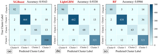
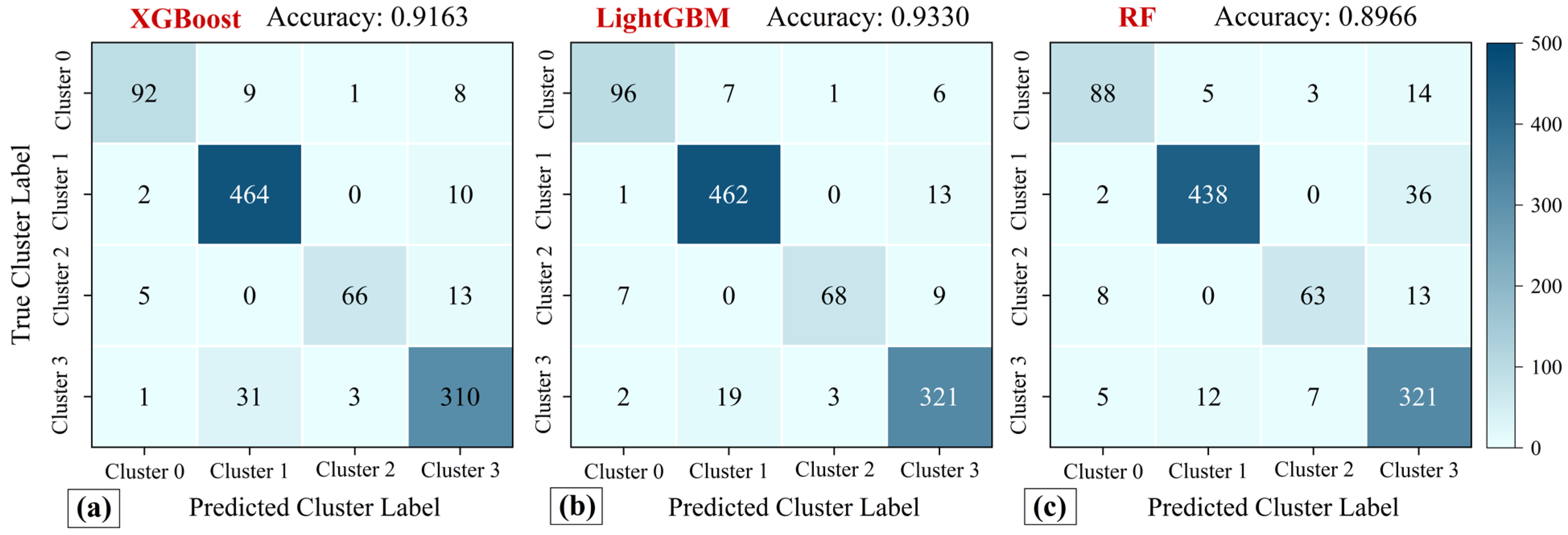
To evaluate the classification performance of the three ensemble learning models under different feature conditions, this study employs confusion matrices to visually present each model’s prediction results across the clustering labels. In addition, performance is quantitatively assessed using precision, recall, and F1-score metrics. After hyperparameter optimization via grid search, all three models achieved classification accuracies exceeding 89% across all cluster categories (see Figure 7). Among the three, the LightGBM model performed the best, achieving an overall accuracy of 93.30%, followed by XGBoost at 91.63%, while Random Forest (RF) trailed slightly at 89.66%.
Figure 7.
Confusion matrices for classification results of different models. (a) XGBoost. (b) LightGBM. (c) Random Forest.
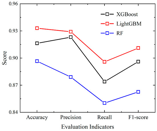
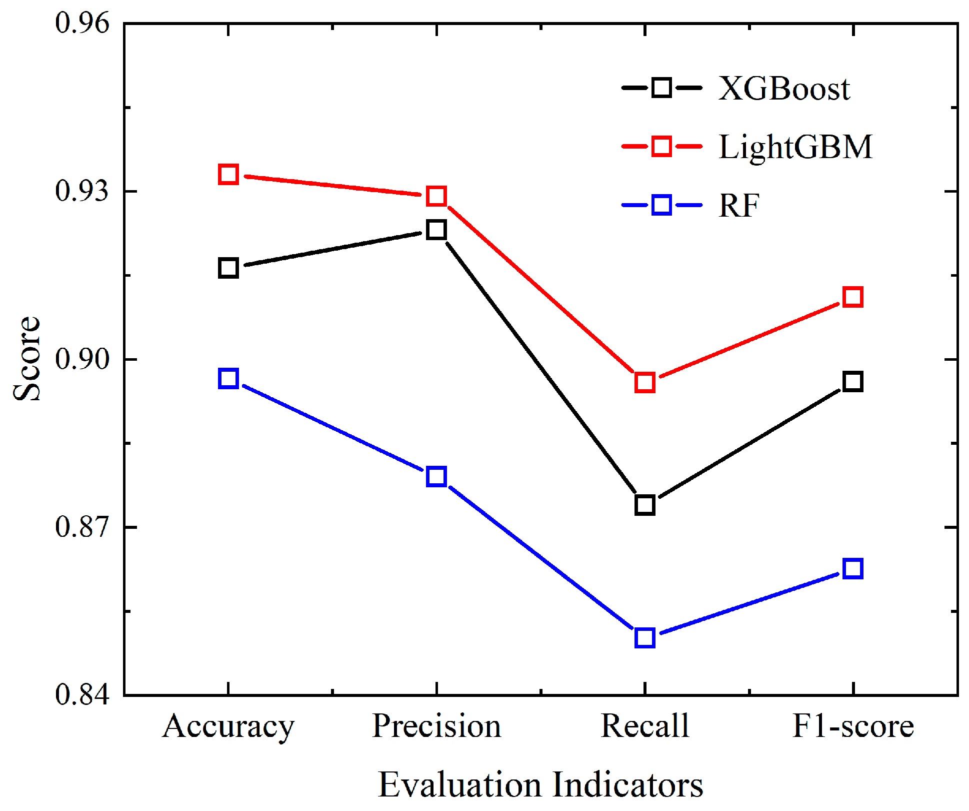
As shown in Figure 8, the three models exhibit consistent trends across different evaluation metrics. LightGBM achieved the best performance across all evaluation metrics, with the highest accuracy (93.30%) and F1-score (0.9111), indicating that the model strikes a well-balanced trade-off between precision and recall. XGBoost also demonstrated strong classification capability, with an F1-score of 0.8960 and a relatively high precision of 0.9231. However, its lower recall rate (0.8739) suggests a more conservative prediction tendency, favoring precision over sensitivity. In comparison, the Random Forest achieves relatively lower scores across the metrics and performs slightly weaker under the data split and settings adopted in this study. It should be emphasized that the ensemble-learning models in this section are used only as supervised surrogates for the unsupervised clustering results—i.e., to test the separability of the cluster labels and to support feature attribution—so the reported accuracy and F1-score mainly reflect internal consistency of the proposed framework. Because unsupervised clustering lacks external “ground-truth labels,” its validity is typically established through a combination of internal evaluation criteria, stability considerations, and verification using external engineering labels [43,44,45]. Accordingly, Section 4.4 further introduces the ATC-63 external labels for cluster-level verification, establishing a testable correspondence between the clustering outcomes and engineering semantics.
Figure 8.
Accuracy of each ensemble model on the training set/test set.
Taken together, the results demonstrate that all three ensemble models exhibit strong clustering recognition capabilities when trained on multi-dimensional feature inputs, with overall evaluation metrics maintained at a high level. These findings further validate that hyperparameter optimization via grid search plays a significant role in enhancing model training effectiveness and classification performance.
4.3. Influence of Feature Indicators on Machine Learning Models
In the preceding feature-engineering stage, a total of 70 seismic-signal features were extracted to cover waveform morphology, energy input, duration process, spectral structure, and signal integrity. While such a high-dimensional feature system helps comprehensively characterize differences among records, it may also introduce information redundancy. To identify features that contribute most to discriminating the clustering labels and to interpret the basis of model decisions, SHapley Additive exPlanations (SHAP) was used to quantify feature contributions in the ensemble models. The discussion is organized around cross-model consensus features and summarized by feature families/physical dimensions, so as to avoid misinterpreting a single-feature ranking as multiple independent engineering criteria. To improve the engineering interpretability of the explainability results, this study does not treat SHAP rankings as “multiple parallel engineering criteria.” Instead, the high-contribution features are grouped by physical dimensions into: (i) peak intensity and energy input, (ii) duration characteristics and cumulative effects, (iii) spectral structure and bandwidth characteristics, (iv) nonstationarity/structural components, and (v) signal integrity. These dimensions correspond to well-recognized response drivers in the near-collapse regime, such as peak demand, cumulative damage, and multi-modal excitation [46]. In addition, indicators such as the “number of zero or missing segments” are used only as signal-integrity and quality-control attributes to prevent incomplete records from distorting cluster boundaries and the resulting interpretations.
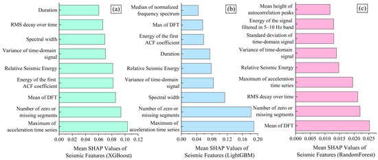
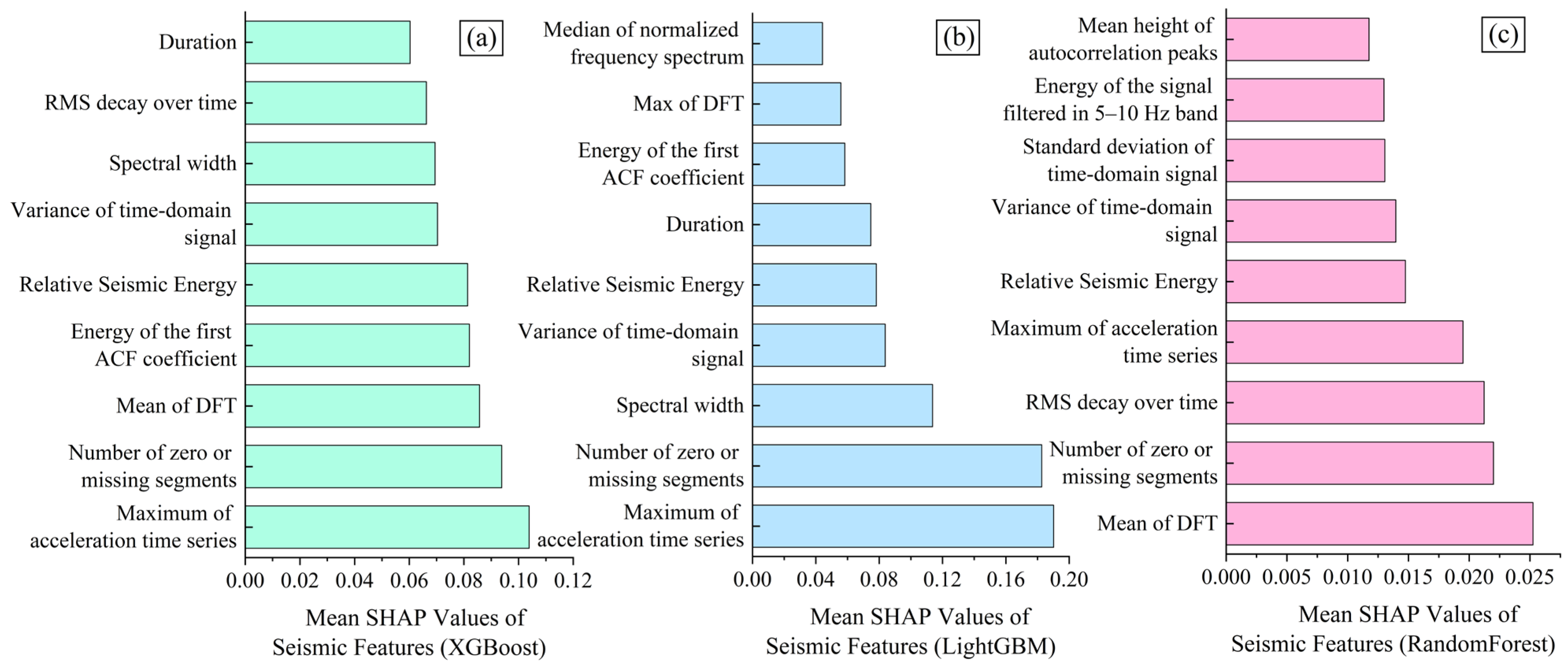
Figure 9 displays the top nine ground motion features with the highest contributions to the overall clustering evaluation across the three models. It can be observed that certain differences in feature rankings still exist among the models. For example, LightGBM places greater emphasis on intensity-related features in the time and frequency domains, such as the maximum of the acceleration time series, the number of zero or missing segments, and spectral width. In contrast, XGBoost exhibits a more balanced SHAP value distribution, with no single feature standing out prominently. Overall, it tends to favor features that reflect waveform stability and frequency–energy distribution, such as the mean of the DFT and the energy of the first autocorrelation (ACF) coefficient; Random Forest shows a relatively balanced feature distribution, with smaller differences in SHAP values across features, indicating that its learning process relies more on the overall statistical characteristics of the signal. Despite differences in model mechanisms, there is a high degree of overlap among the top nine features identified by the three ensemble models, indicating a strong consensus in their understanding of the underlying structure of seismic signal recognition.
Figure 9.
Ranking of seismic wave characteristic parameters for the three ensemble models (top 9 retained). (a) XGBoost. (b) LightGBM. (c) Random Forest.
As shown in Table 2, these high-importance features span multiple physical dimensions of ground motion, including time-domain intensity, frequency-domain structure, energy density, and signal integrity, forming the core basis for the models’ clustering decisions. It is worth noting that features such as the Maximum of acceleration time series and Relative Seismic Energy not only rank highly across all models but were also validated in the earlier engineering label analysis as key indicators of hazardous ground motions. This further indicates that the clustering decision logic learned by the models exhibits strong engineering interpretability and physical consistency.
Table 2.
Common major contributing features of LightGBM, XGBoost, and RandomForest models.
Building upon the identification of core features with high consistency across models, this study further conducts an in-depth analysis of the contribution differences of these key features across different clusters, using the previously identified best-performing model, LightGBM.
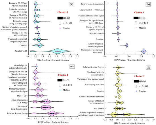
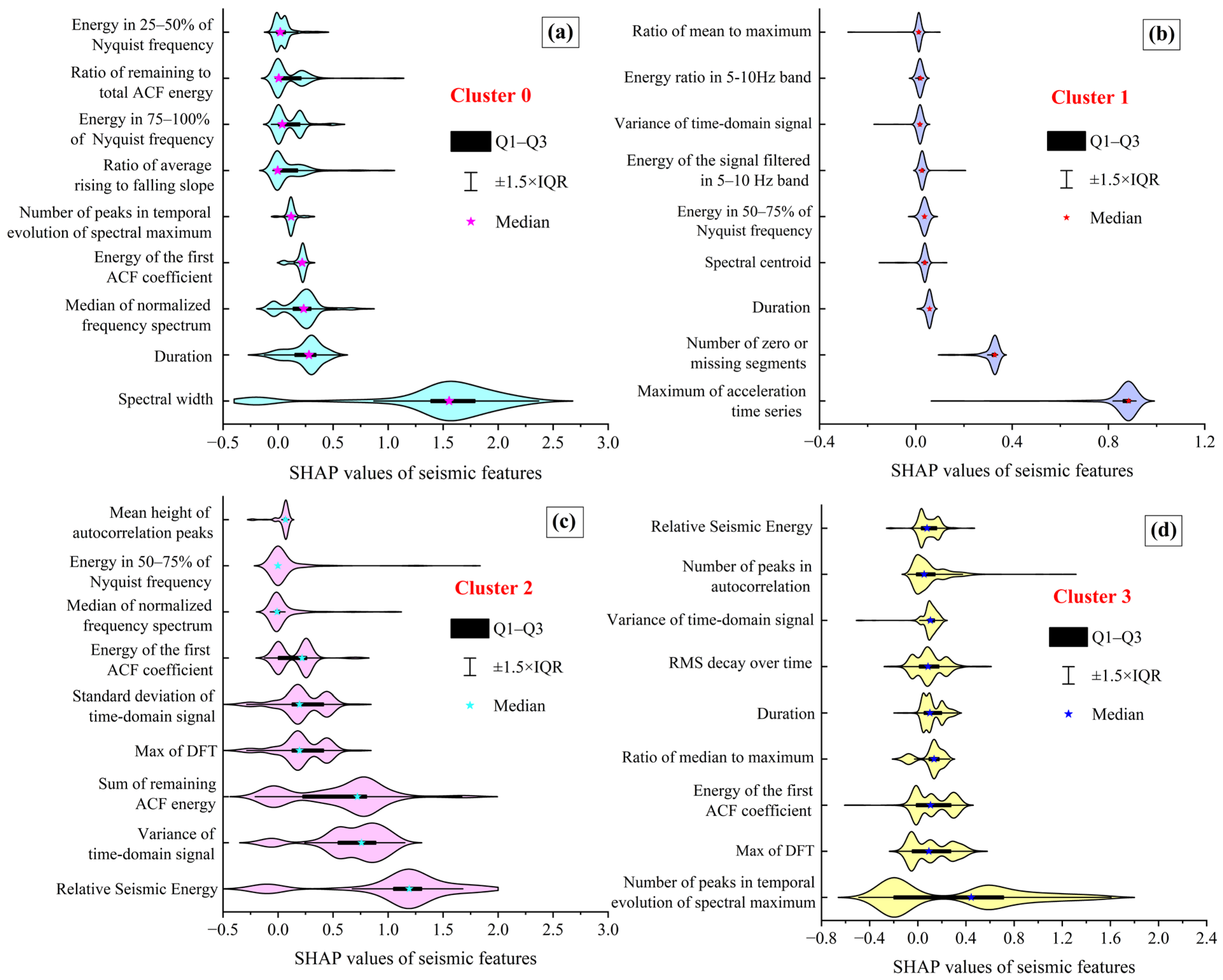
This study extracted the top nine ground motion features ranked by SHAP values within each cluster as computed by the LightGBM model, along with their corresponding distributions, as shown in Figure 10. The clusters exhibit markedly different feature ranking structures and SHAP value distributions, reflecting their intrinsic distinctions in the physical attributes of ground motions. In Cluster 0, the SHAP value distribution spans a relatively wide range, with certain samples exhibiting notable characteristics in high-frequency extensibility. However, the overall feature values tend to be moderate, lacking pronounced extremity. The top-ranked features in this cluster include Spectral width and Median of normalized frequency spectrum, indicating that the waveforms exhibit a certain degree of frequency structure extensibility and moderate volatility. This aligns with the earlier characterization of the cluster as representing “moderate intensity with moderate spectral breadth.”
Figure 10.
Ranking of seismic wave characteristic parameters for the four clusters in the LightGBM model (top 9 retained). (a) Cluster 0. (b) Cluster 1. (c) Cluster 2. (d) Cluster 3.
Cluster 1 exhibits the most concentrated SHAP value distribution, with overall low feature contribution values. The model primarily relies on low-amplitude and discontinuity-related features, such as Maximum of acceleration time series and Number of zero or missing segments, for identification. It should be noted that the Number of zero or missing segments is a feature related to record continuity/completeness. Its relatively high contribution is mainly used to distinguish the sparse/intermittent low-amplitude records within this cluster (Figure 10) and should not be interpreted as a dominant factor governing the collapse mechanism. Combined with the statistical analysis results from Figure 6, this cluster primarily consists of low-energy, stable, and sparse waveforms characteristic of microseisms or far-field ground motions, making it the least hazardous among the clusters. Key features for Cluster 3 include Number of peaks in temporal evolution of spectral maximum and Max of DFT, with SHAP values showing relatively concentrated distributions. This suggests that the identification of signals in this cluster relies on the stability of time–frequency domain characteristics. The waveforms are characterized by moderate amplitude and good signal continuity, representing stable, medium-intensity ground motions.
In contrast, Cluster 2 exhibits the most pronounced feature extremity, with several SHAP values among its top nine features significantly higher than those of other clusters and showing a markedly right-skewed distribution. This indicates that these features play a decisive role in the model’s identification of this class of strong ground motion signals. Its core features include Relative Seismic Energy (energy density), Variance of time-domain signal (waveform volatility), Max of DFT (dominance of high-frequency amplitude), as well as Sum of remaining ACF energy and Energy of the first ACF coefficient (periodicity and energy persistence). Together, these indicators form the high-risk signal profile of Cluster 2, characterized by a combination of high amplitude, high energy, broad frequency bandwidth, and strong nonstationarity—hallmarks of intense seismic events. This result is consistent with the earlier clustering structure analysis and engineering label validation, and further explains the hazard potential of Cluster 2 from the perspective of feature contribution.
4.4. Engineering Validation of Collapse-Oriented Clustering
Table 3 reports the enrichment of the ATC-63 far-field collapse records across the four unsupervised clusters. Cluster 2 has an enrichment ratio ERj ≈ 10.96, with the proportion of ATC-63 records far exceeding the full-database baseline (p ≈ 3.1 × 10⁻²⁰, FDR-adjusted q ≈ 1.24 × 10⁻¹⁹), while the other three clusters have ERj < 1 or close to 0 and show no enrichment. This indicates that the adverse waveform and statistical characteristics of Cluster 2 are highly consistent with the distribution of the engineering labels, so it can be identified as the collapse-sensitive phenotype cluster (COP). Overall, the clustering structure shows clear consistency and separability with collapse-related labels, providing a statistical and interpretable basis for expanding collapse-oriented ground-motion libraries.
Table 3.
Cluster-level enrichment test of ATC-63 far-field strong-motion engineering labels.
Based on the waveform shapes and statistical characteristics of each cluster, this study first performs a systematic comparison. The ATC-63 far-field records are then used as engineering labels to conduct cluster-level enrichment and coverage tests. On this unified statistical basis, an engineering-oriented classification and naming scheme is proposed for the four clusters to support record selection and scenario description in expanded ground-motion libraries. The key waveform features and engineering interpretations are summarized in Table 4. In this scheme, Cluster 0 corresponds to short-duration, moderate-energy motions (SDME), Cluster 1 to far-field long-tail motions (FFLT), Cluster 2 to collapse-sensitive motions (COP), and Cluster 3 to near-field motions with multi-burst energy release (NFMB).
Table 4.
In-cluster distribution of engineering labeled samples.
In addition, the proposed framework is designed for identifying and expanding a collapse-oriented candidate ground-motion library, rather than conducting direct NLTHA/IDA benchmarking using a specific structural archetype. Structure-prototype-based baseline comparisons (e.g., against conventional CMS/GCIM or spectrum-shape-based selection approaches) are therefore left for future work and will be carried out once the structural type and analysis protocol are clearly defined. Within the current scope, we establish a testable alignment between the clustering results and engineering semantics through cluster-level enrichment/coverage tests using the ATC-63 record set as an external engineering label.
Overall, the unsupervised clustering model can cover most known hazardous motions and reveal additional “hidden high-risk” signals beyond current design codes, providing technical support for ground-motion screening, fragility modelling and risk identification.
5. Conclusions
This study developed a hazardous ground-motion identification framework for structural collapse assessment. STA/LTA was used for event detection and feature extraction, GMM for unsupervised clustering, and ensemble learning with SHAP to interpret the clustering. The ATC-63 far-field record set was then used for cluster-level enrichment and coverage checks to identify the collapse-sensitive cluster (COP). The main findings are as follows:
- (1)
- Unsupervised clustering can effectively separate ground motions with different hazard levels. Using a Gaussian mixture model (GMM) on multi-domain features (time, frequency, time–frequency and signal quality), four waveform clusters with clear physical differences are obtained. Comparison of PGA, Arias intensity, 5–95% Energy Duration, time-domain variance and Rrup shows that Cluster 2 has stronger input and longer effective duration, placing it on the unfavorable side in several dimensions and indicating higher engineering hazard.
- (2)
- The evaluation results of the ensemble models validate the separability and learnability of the clustering labels. All three ensemble learning models developed in this study—LightGBM, XGBoost, and Random Forest—demonstrated strong performance in classifying the clustering labels, with F1-scores exceeding 0.89. Among them, LightGBM achieved the best results, with an overall accuracy of 93.30% and an F1-score of 0.9111. These outcomes indicate that the clustered ground motion signals possess well-defined feature boundaries and exhibit high discriminability.
- (3)
- SHAP analysis reveals the feature-level differences among clusters, further enhancing the engineering interpretability of the clustering structure. SHAP-based feature contribution analysis of the LightGBM model reveals significant differences in the contribution patterns of key features across different clusters. Cluster 0 is primarily characterized by spectral extensibility and moderate waveform volatility; Cluster 1 exhibits low-energy, sparse signals indicative of low-hazard waveforms; and Cluster 3 displays moderate intensity with a stable frequency-domain structure. In contrast, Cluster 2 stands out prominently in features such as relative seismic energy, time-domain volatility, and frequency dominance, forming a characteristic spectrum of strong-motion hazard signatures.
- (4)
- Identification and engineering classification of collapse-sensitive motions. Enrichment and coverage tests with ATC-63 labels show that Cluster 2 is strongly enriched in collapse-related records and has the highest coverage (enrichment ratio 10.96), so it can be taken as the collapse-sensitive phenotype cluster (COP). The engineering-oriented cluster names (SDME/FFLT/COP/NFMB) are consistent with their waveform and statistical features and provide a clear, reviewable basis for record selection and ground-motion library expansion in collapse assessment.
Author Contributions
Conceptualization, X.Z. and W.P.; methodology, X.Z.; software, X.Z.; validation, X.Z. and W.P.; formal analysis, X.Z.; investigation, X.Z.; resources, L.Y.; data curation, X.Z.; writing—original draft preparation, X.Z.; writing—review and editing, W.P. and L.Y.; visualization, X.Z.; supervision, W.P. and L.Y.; project administration, W.P. All authors have read and agreed to the published version of the manuscript.
Funding
This research was funded by the National Natural Science Foundation of China, grant number 42367025, and the National Natural Science Foundation of China, grant number 32060368.
Data Availability Statement
The original contributions presented in this study are included in the article. Further inquiries can be directed to the corresponding author.
Conflicts of Interest
The authors declare no conflicts of interest.
Abbreviations
The following abbreviations are used in this manuscript:
| SHAP | SHapley Additive exPlanations |
| GMM | Gaussian Mixture Models |
| BIC | Bayesian Information Criterion |
| AIC | Akaike Information Criterion |
Appendix A
Definitions and Physical Interpretations of Seismic Wave Feature Parameters
Table A1.
Time-domain features.
Table A2.
Frequency-domain features.
Table A3.
Time–frequency features.
Table A4.
Signal quality features.
References
- Kim, J.; Kim, T. Efficient seismic fragility analysis considering uncertainties in structural systems and ground motions. Earthq. Eng. Struct. Dyn. 2025, 54, 206–226. [Google Scholar] [CrossRef] [Scilit]
- Applied Technology Council. Quantification of Building Seismic Performance Factors; US Department of Homeland Security, FEMA: Washington, DC, USA, 2009.
- Bassman, T.J.; Zhong, K.; Baker, J.W. Ground motion selection using code-compliant conditional mean spectra: Effects of conditioning period and amplitude constraints. In Proceedings of the 12th National Conference on Earthquake Engineering, Salt Lake City, UT, USA, 27 June–1 July 2022. [Google Scholar]
- FEMA P-695 (ATC-63 Project); Quantification of Building Seismic Performance Factors. Federal Emergency Management Agency: Washington, DC, USA, 2009.
- Park, S.; Seo, D.; Jung, K.; Kim, J. Study on the Uncertainty of Input Variables in Seismic Fragility Curves Based on the Number of Ground Motions. Appl. Sci. 2024, 14, 11787. [Google Scholar] [CrossRef] [Scilit]
- Safiey, A.; Majdalaweyh, S.; Pang, W. Assessing the Impact of Ground Motion Duration on Losses in Typical Modern Steel Moment Frames. Buildings 2024, 14, 1373. [Google Scholar] [CrossRef] [Scilit]
- Zhang, Y.; Shen, R.; Sun, B.; Liu, T.; Shi, Y.; Li, L. Selection of ground motion intensity measures in fragility analysis of a mega-scale steel frame structure at separate limit states: A case study. Buildings 2022, 12, 1530. [Google Scholar] [CrossRef] [Scilit]
- Baker, J.W. Conditional mean spectrum: Tool for ground-motion selection. J. Struct. Eng. 2011, 137, 322–331. [Google Scholar] [CrossRef] [Scilit]
- Bradley, B.A. A generalized conditional intensity measure approach and holistic ground-motion selection. Earthq. Eng. Struct. Dyn. 2010, 39, 1321–1342. [Google Scholar] [CrossRef] [Scilit]
- Liu, T.; Han, Y.; Wang, Q.; Yuan, Y. Assessing Ground Motion Intensity Measures and Structural Damage Measures in Underground Structures: A Finite Element Analysis of the Daikai Subway Station. Appl. Sci. 2024, 14, 5491. [Google Scholar] [CrossRef] [Scilit]
- Aquib, T.A.; Sivasubramonian, J.; Mai, P.M. Analysis of Ground Motion Intensity Measures and Selection Techniques for Estimating Building Response. Appl. Sci. 2022, 12, 12089. [Google Scholar] [CrossRef] [Scilit]
- Lindsey, N.J.; Martin, E.R.; Dreger, D.S.; Freifeld, B.; Cole, S.; James, S.R.; Biondi, B.L.; Ajo-Franklin, J.B. Fiber-Optic Network Observations of Earthquake Wavefields. Geophys. Res. Lett. 2017, 44, 11792–11799. [Google Scholar] [CrossRef] [Scilit]
- Liu, G.; Li, R.; He, J.; Li, W.; Lu, J.; Long, W.; Gao, P.; Cai, G.; Tang, M. Scaling relation of earthquake seismic data. Phys. A Stat. Mech. Appl. 2018, 492, 2092–2102. [Google Scholar] [CrossRef] [Scilit]
- Chen, Y. Automatic microseismic event picking via unsupervised machine learning. Geophys. J. Int. 2020, 222, 1750–1764. [Google Scholar] [CrossRef] [Scilit]
- Hibert, C.; Provost, F.; Malet, J.-P.; Maggi, A.; Stumpf, A.; Ferrazzini, V. Automatic identification of rockfalls and volcano-tectonic earthquakes at the Piton de la Fournaise volcano using a Random Forest algorithm. J. Volcanol. Geotherm. Res. 2017, 340, 130–142. [Google Scholar] [CrossRef] [Scilit]
- Morin, A.; Giroux, B.; Gauthier, F. Characterizing Seismic Activity from a Rock Cliff with Unsupervised Learning. J. Geophys. Res. Earth Surf. 2024, 129, e2024JF007799. [Google Scholar] [CrossRef] [Scilit]
- Yin, X.; Liu, F.; Cai, R.; Yang, X.; Zhang, X.; Ning, M.; Shen, S. Research on Seismic Signal Analysis Based on Machine Learning. Appl. Sci. 2022, 12, 8389. [Google Scholar] [CrossRef] [Scilit]
- Kim, T.; Kwon, O.S.; Song, J. Clustering-based adaptive ground motion selection algorithm for efficient estimation of structural fragilities. Earthq. Eng. Struct. Dyn. 2021, 50, 1755–1776. [Google Scholar] [CrossRef] [Scilit]
- Asgarkhani, N.; Kazemi, F.; Jankowski, R.; Formisano, A. Dynamic ensemble-learning model for seismic risk assessment of masonry infilled steel structures incorporating soil-foundation-structure interaction. Reliab. Eng. Syst. Saf. 2025, 267, 111839. [Google Scholar] [CrossRef] [Scilit]
- Maggi, A.; Ferrazzini, V.; Hibert, C.; Beauducel, F.; Boissier, P.; Amemoutou, A. Implementation of a Multistation Approach for Automated Event Classification at Piton de la Fournaise Volcano. Seismol. Res. Lett. 2017, 88, 878–891. [Google Scholar] [CrossRef] [Scilit]
- Gao, Y.; Zhao, P.; Li, G.; Li, H. Seismic noise attenuation by signal reconstruction: An unsupervised machine learning approach. Geophys. Prospect. 2021, 69, 984–1002. [Google Scholar] [CrossRef] [Scilit]
- Shi, P.; Seydoux, L.; Poli, P. Unsupervised Learning of Seismic Wavefield Features: Clustering Continuous Array Seismic Data During the 2009 L’Aquila Earthquake. J. Geophys. Res. Solid Earth 2021, 126, e2020JB020506. [Google Scholar] [CrossRef] [Scilit]
- Langet, N.; Silverberg, F.M.J. Automated classification of seismic signals recorded on the Åknes rock slope, Western Norway, using a convolutional neural network. Earth Surf. Dyn. 2023, 11, 89–115. [Google Scholar] [CrossRef] [Scilit]
- Seydoux, L.; Balestriero, R.; Poli, P.; de Hoop, M.; Campillo, M.; Baraniuk, R. Clustering earthquake signals and background noises in continuous seismic data with unsupervised deep learning. Nat. Commun. 2020, 11, 3972. [Google Scholar] [CrossRef] [Scilit]
- Mousavi, S.M.; Zhu, W.; Ellsworth, W.; Beroza, G. Unsupervised Clustering of Seismic Signals Using Deep Convolutional Autoencoders. IEEE Geosci. Remote Sens. Lett. 2019, 16, 1693–1697. [Google Scholar] [CrossRef] [Scilit]
- Lundberg, S.M.; Erion, G.; Chen, H.; DeGrave, A.; Prutkin, J.M.; Nair, B.; Katz, R.; Himmelfarb, J.; Bansal, N.; Lee, S.-I. From local explanations to global understanding with explainable AI for trees. Nat. Mach. Intell. 2020, 2, 56–67. [Google Scholar] [CrossRef] [Scilit]
- Brandsæter, A.; Glad, I.K. Shapley values for cluster importance. Data Min. Knowl. Discov. 2024, 38, 2633–2664. [Google Scholar] [CrossRef] [Scilit]
- Cohen, J.; Huan, X.; Ni, J. Shapley-based explainable AI for clustering applications in fault diagnosis and prognosis. J. Intell. Manuf. 2024, 35, 4071–4086. [Google Scholar] [CrossRef] [Scilit]
- ASCE/SEI 7-22; Minimum Design Loads and Associated Criteria for Buildings and Other Structures. ASCE: Reston, VA, USA, 2022.
- EN 1998-1:2004+A1:2013; Eurocode 8: Design of Structures for Earthquake Resistance—Part 1: General Rules, Seismic Actions and Rules for Buildings. CEN: Brussels, Belgium, 2013.
- Akram, J.; Eaton, D.W. A review and appraisal of arrival-time picking methods for downhole microseismic data. Geophysics 2016, 81, KS71–KS91. [Google Scholar] [CrossRef] [Scilit]
- Latto, R.B.; Turner, R.J.; Reading, A.M.; Winberry, J.P. Towards the systematic reconnaissance of seismic signals from glaciers and ice sheets—Part 1: Event detection for cryoseismology. Cryosphere 2024, 18, 2061–2079. [Google Scholar] [CrossRef] [Scilit]
- Provost, F.; Hibert, C.; Malet, J.P. Automatic classification of endogenous landslide seismicity using the Random Forest supervised classifier. Geophys. Res. Lett. 2017, 44, 113–120. [Google Scholar] [CrossRef] [Scilit]
- An, P.; Wang, Z.; Zhang, C. Ensemble unsupervised autoencoders and Gaussian mixture model for cyberattack detection. Inf. Process. Manag. 2022, 59, 102844. [Google Scholar] [CrossRef] [Scilit]
- Akaike, H. A new look at the statistical model identification. IEEE Trans. Autom. Control 1974, 19, 716–723. [Google Scholar] [CrossRef] [Scilit]
- Wan, H.; Wang, H.; Scotney, B.; Liu, J. A Novel Gaussian Mixture Model for Classification. In Proceedings of the 2019 IEEE International Conference on Systems, Man and Cybernetics (SMC), Bari, Italy, 6–9 October 2019; IEEE: Bari, Italy, 2019; pp. 3298–3303. [Google Scholar]
- Schwarz, G. Estimating the Dimension of a Model. Ann. Stat. 1978, 6, 461–464. [Google Scholar] [CrossRef] [Scilit]
- Ke, G.; Meng, Q.; Finley, T.; Wang, T.; Chen, W.; Ma, W.; Ye, Q.; Liu, T.-Y. LightGBM: A Highly Efficient Gradient Boosting Decision Tree. In Proceedings of the 31st Conference on Neural Information Processing Systems (NIPS 2017), Long Beach, CA, USA, 4–9 December 2017; Curran Associates, Inc.: Red Hook, NY, USA, 2017; Volume 30. [Google Scholar]
- Breiman, L. Random Forests. Mach. Learn. 2001, 45, 5–32. [Google Scholar] [CrossRef] [Scilit]
- Chen, T.; Guestrin, C. XGBoost: A Scalable Tree Boosting System. In Proceedings of the 22nd ACM SIGKDD International Conference on Knowledge Discovery and Data Mining, San Francisco, CA, USA, 13–17 August 2016; Association for Computing Machinery: New York, NY, USA, 2016; pp. 785–794. [Google Scholar]
- Štrumbelj, E.; Kononenko, I. Explaining prediction models and individual predictions with feature contributions. Knowl. Inf. Syst. 2014, 41, 647–665. [Google Scholar] [CrossRef] [Scilit]
- Louhichi, M.; Nesmaoui, R.; Mbarek, M.; Lazaar, M. Shapley Values for Explaining the Black Box Nature of Machine Learning Model Clustering. Procedia Comput. Sci. 2023, 220, 806–811. [Google Scholar] [CrossRef] [Scilit]
- Jain, A.K. Data clustering: 50 years beyond K-means. Pattern Recognit. Lett. 2010, 31, 651–666. [Google Scholar] [CrossRef] [Scilit]
- Von Luxburg, U. Clustering stability: An overview. Found. Trends® Mach. Learn. 2010, 2, 235–274. [Google Scholar] [CrossRef] [Scilit]
- Hennig, C. What are the true clusters? Pattern Recognit. Lett. 2015, 64, 53–62. [Google Scholar] [CrossRef] [Scilit]
- Luco, N.; Cornell, C.A. Structure-specific scalar intensity measures for near-source and ordinary earthquake ground motions. Earthq. Spectra 2007, 23, 357–392. [Google Scholar] [CrossRef] [Scilit]

Disclaimer/Publisher’s Note: The statements, opinions and data contained in all publications are solely those of the individual author(s) and contributor(s) and not of MDPI and/or the editor(s). MDPI and/or the editor(s) disclaim responsibility for any injury to people or property resulting from any ideas, methods, instructions or products referred to in the content. |
© 2026 by the authors. Licensee MDPI, Basel, Switzerland. This article is an open access article distributed under the terms and conditions of the Creative Commons Attribution (CC BY) license.