


Abstract
Fifth-generation district heating and cooling (5GDHC) systems have attracted increasing attention because they can supply heating and cooling simultaneously, enable buildings to act as thermal prosumers, and facilitate the recovery of low-grade waste heat. Because these networks operate near ambient temperature, their temperature can be modulated over a relatively wide range in both winter and summer, creating the potential to use the pipe network for both heat and cold storage. However, the economic value of using this inherent thermal capacity and the benefit of increasing it through pipe enlargement remain unclear. This study develops a dynamic thermo-hydraulic optimization framework that represents bidirectional flow, water and ground thermal states, temperature-dependent heat-pump and chiller performance, pumping electricity, and annualized system costs. A genetic algorithm is used offline to compare daily-constant and predictive network-temperature control at three pipe-capacity levels in a synthetic 5GDHC system developed using Beijing weather and tariff data. Predictive control reduced the annualized cost at all three pipe-capacity levels, with savings ranging from 0.17% to 0.52%. Reductions in monthly demand charges and active-equipment capacity costs provided most of the economic benefit, whereas the energy charge changed only slightly or increased. Increasing every pipe by one or two catalog sizes raised the network water volume by 32.1% and 69.5% and reduced pumping electricity by 51.8% and 74.0%, but increased the annualized cost by 0.14% and 0.44%, respectively. The results show that the thermal capacity already available in a 5GDHC network can provide modest operational flexibility, but enlarging pipes solely to obtain additional thermal storage did not show a substantial economic advantage in the investigated case.
1. Introduction
Buildings account for around 30% of global energy demand and approximately 37% of global carbon dioxide emissions [1]. Consequently, the building sector has a central role in global decarbonization. Heating and cooling are particularly important: heating alone accounts for around half of building energy use [2], whereas global residential space-cooling energy use is projected to triple between 2020 and 2050 under a current-policy reference scenario, driven by warmer climates, expanding floor area, rising incomes, and wider access to air conditioning [3]. Improving the efficiency of building heating and cooling and replacing carbon-intensive energy sources are therefore essential components of the energy transition.
District heating and cooling (DHC) systems are considered a promising approach for the efficient supply of heating and cooling. Unlike individual building systems, a DHC system supplies multiple buildings through shared thermal infrastructure. At the district scale, this shared infrastructure can exploit source diversity and economies of scale, recover heat that would otherwise be rejected, and integrate renewable and low-grade thermal sources that are difficult to use at the building level [4,5]. In recent years, fifth-generation district heating and cooling (5GDHC) has emerged as a low-temperature and bidirectional form of DHC. Unlike conventional DHC systems, 5GDHC uses a near-ambient water network together with decentralized heat pumps, chillers, and direct heat exchangers to deliver the temperatures required by individual buildings [6]. This configuration allows buildings to act as thermal prosumers: cooling buildings reject heat that can support heating loads, while heating buildings return lower-temperature water that can support cooling loads through the shared network.
DHC systems are also increasingly studied as flexible energy assets. Conventional flexibility is commonly provided by dedicated thermal energy storage systems or batteries. For example, Wang et al. [7] used a TRNSYS model to evaluate a radiation-enhanced thermal diode tank that provided cooling water to the condenser of a refrigeration and air-conditioning system. The pipe network itself, however, already contains a large volume of water that can store sensible heat across hours without a separate storage device, and most studies of this flexibility have focused on district heating, where supply-temperature or flow-rate control is used to precharge the network before a demand peak [8,9,10,11]. By contrast, conventional district-cooling networks distribute chilled water close to the temperatures required by buildings, leaving limited scope for further downward adjustment. District-cooling storage studies therefore generally examine separate chilled-water, ice, or latent-heat storage systems rather than the distribution pipes themselves [12,13]. A 5GDHC network operates near ambient temperature rather than near the final delivery temperature of either heating or cooling. The survey by Buffa et al. reported several closed-loop 5GDHC systems with operating temperature ranges of 20–27 K, e.g., 0–25 °C and 8–35 °C [6]. This operating range allows a 5GDHC network to shift its temperature upward or downward and potentially provide heat or cold flexibility through its water volume.
Existing 5GDHC research has usually focused on system design and system operation. For system design, Wirtz et al. [14] formulated a mathematical optimization method for network layout and component sizing. Maccarini et al. [15] quantified how building-side temperature requirements affect both energy performance and network sizing, while Mans et al. [16] developed an open-source framework for dynamic low-temperature network simulation. Pompei et al. [17] showed that generation and storage capacities must be evaluated together with their operating conditions, and Elhafaia et al. [18] demonstrated that pipe diameter simultaneously affects investment, pumping, heat transfer, and hydraulic feasibility.
For system operation, Zhang et al. [19] compared constant, staged, and free-floating network-temperature strategies, and Dai et al. [20] reviewed the wider range of control methods used in 5GDHC systems. Wirtz et al. [21] formulated an operation optimization model in which network-temperature trajectories shift energy and reduce operating cost. Buffa et al. [22] applied predictive control to building-sited storage under time-of-use tariffs, while Quirosa et al. [23] assessed an ultra-low-temperature network as storage for renewable integration.
Despite these advances, few studies have examined the pipe network itself as a thermal storage resource in 5GDHC systems. Previous studies indicate that varying the network temperature can shift electrical demand and potentially reduce demand charges, but the economic value of exploiting the thermal capacity of the network remains unclear. Furthermore, increasing pipe diameter can increase the water volume and hence the storage capacity of the network, but it also raises the initial pipe investment. Whether the resulting operating-cost savings can offset this additional investment has not been sufficiently examined.
To address these questions, this study develops a thermo-hydraulic optimization framework for two-pipe 5GDHC systems. The framework considers mass and energy balances, hydraulic constraints, temperature-dependent equipment performance, and the thermal capacity of the network water. The resulting mixed-variable nonconvex problem is solved using a genetic algorithm. The framework is applied to a synthetic case to evaluate the economic value of pipe-network thermal storage and of increasing pipe diameter to provide additional storage capacity.
The main contributions of this study are as follows:
- A dynamic thermo-hydraulic optimization framework is developed to represent the thermal capacity of the pipe water and surrounding ground, bidirectional flow, and temperature-dependent equipment performance in a non-tree 5GDHC network.
- A controlled comparison between daily-constant and predictive network-temperature control quantifies the operational value of this thermal capacity and decomposes the resulting savings into energy, maximum-demand, and equipment-capacity cost components.
- Pipe enlargement is evaluated as a thermal-storage investment by comparing the value of additional network thermal capacity and reduced hydraulic resistance with the additional annualized pipe cost.
The remainder of this paper is organized as follows. Section 2 presents the optimization model, including the objective function, decision variables, and physical constraints. Section 3 introduces the synthetic case and analyzes the results. Section 4 discusses the economic mechanisms and practical implications. Section 5 presents the main conclusions, limitations, and directions for future research.
2. Methodology
2.1. System Configuration and Modeling Assumptions
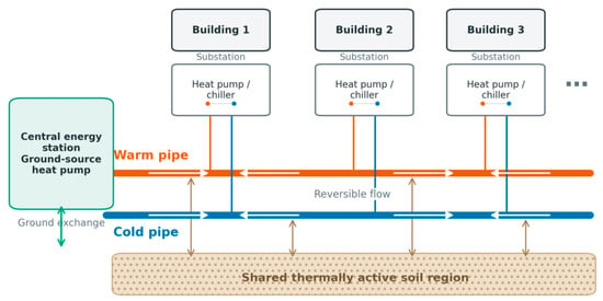
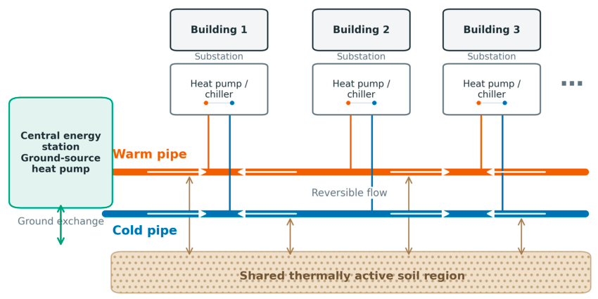
Figure 1 illustrates the modeled system configuration. The system adopts the conventional two-pipe configuration of a 5GDHC network, consisting of a warm pipe and a cold pipe arranged in a ring topology. Flow directions in individual pipe sections can change as buildings alternate between extracting heat from and rejecting heat to the network. Each building substation contains a heat pump or chiller connected to both pipes. A central energy station is connected to the network to inject or remove heat and maintain the warm- and cold-pipe temperatures within their allowable ranges. Both pipes exchange heat with the surrounding soil, which provides additional thermal capacity together with the water contained in the network.
Figure 1.
Configuration and thermal interactions of the modeled 5GDHC system.
The baseline pipe diameters are selected using a maximum specific friction pressure loss criterion, following the engineering practice adopted in our previous studies [24,25]. In a ring network, the nodal mass-balance equations alone form an underdetermined system. The hourly pipe flow rates are therefore calculated by solving the nodal mass-balance equations together with the loop pressure-balance equations. Because friction pressure loss depends on both flow rate and pipe diameter, the diameter of each pipe section should be selected from a predefined series of standard nominal diameters and represented as a discrete design variable. For each network section, the paired warm and cold pipes are assumed to have identical lengths and diameters and equal hourly volumetric flow-rate magnitudes.
2.2. Optimization Setup
The proposed optimization framework evaluates pipe design and station-temperature control within a common nonlinear thermo-hydraulic model. The model inputs include the network topology and route lengths, building heating and cooling loads, ground temperature, equipment performance, electricity tariffs, and component costs. The complete decision vector contains the pipe option ze selected for each network section and the mean network temperature θt scheduled for each control period. Both decisions are optimized in the design experiments. In the operating comparisons, the pipe options are fixed and only the station-temperature trajectory is optimized or prescribed.
Each network section selects one option from a predefined set of pipe sizes:
The internal diameter, flow area, hydraulic resistance, water volume, pipe investment, and pipe–ground thermal parameters are determined by the selected pipe option:
where denotes the parameter set associated with pipe option ze.
Following the temperature representation adopted by Wirtz et al. [21], the temperatures supplied to the warm and cold pipes are expressed using the mean network temperature and a prescribed temperature difference:
where and are the warm- and cold-pipe temperatures at the central energy station, respectively, and δt is the prescribed temperature difference between the two pipes. Fixing δt prevents temperature-difference control from introducing an additional change in network flow and pumping demand. The comparison can therefore focus on the effects of mean-temperature scheduling and the thermal capacity of the network.
To limit the number of control variables in the annual optimization, the 365 calendar days are grouped into 12 classes using K-means clustering based on their daily heating and cooling load profiles and ground-temperature information, following Su et al. [26]. Days within each class share a nominal station-temperature schedule. For predictive control, six temperature points are optimized for each class, reducing the number of temperature variables from 2190 to 72. Each candidate schedule is then evaluated over all 8760 h using the original hourly loads, ground temperatures, and electricity prices, with the pipe-water and ground thermal states carried continuously between hours.
The optimization objective is to minimize the total annualized system cost:
where Cp is the annualized pipe investment, Cs is the annualized central heat-pump/chiller capacity cost, Ct is the annualized transformer capacity cost, Ce is the electricity consumption cost, and Cd is the demand charge.
Capital investments are annualized using the capital recovery factor a:
where r is the discount rate and N is the economic lifetime. Because each network section contains one warm pipe and one cold pipe, the annualized pipe investment is
where Le is the route length of section e, and is the unit cost of the selected pipe option.
The required central heat-pump/chiller capacity and transformer capacity are determined from the maximum central-station heat exchange and maximum electrical demand over the full year:
Their annualized costs are
where cs is the unit capacity cost of the central heat-pump/chiller equipment, ct is the assumed transformer investment per unit of electrical capacity, and β is the fraction of this investment allocated to the district system. Here, T contains all 8760 billable hours, and Ta contains the hours with active heat-pump or chiller operation.
The annual electricity consumption cost is calculated from the 8760 hourly inputs:
where t denotes an hour of the chronological year, πt is the corresponding electricity price, and Δt is the time-step duration.
The demand charge is calculated separately for each calendar month using its actual maximum electrical demand:
where cd is the monthly demand-charge rate and Tm is the set of hours in calendar month m.
2.3. Component Performance Model
The coefficients of performance (COPs) of the building and central-station equipment are calculated using the generalized component model of Jensen et al. [27], with the refrigerant parameters adopted by Wirtz et al. [14]. For a constant-capacity stream, the entropic mean temperature is
where the temperatures are expressed in kelvin. Define
where the subscripts h and c denote the higher- and lower-temperature streams, respectively. The refrigerant-side temperature corrections and compressor-loss ratio are calculated as
The water-side entropic mean temperatures are then corrected to the refrigerant condensing and evaporating temperatures:
where ΔTpp is the heat-exchanger pinch temperature difference and ω is the compressor-loss ratio. The condenser-side COP is
where ηis is the isentropic efficiency and fQ is the fractional heat loss. The heating COP is equal to the condenser-side COP, whereas the cooling COP is evaluated on the evaporator side:
The correction coefficients, isentropic efficiencies, fractional heat losses, and any imposed COP cap are specified in the case study.
For direct cooling, the local higher and lower pipe temperatures are defined as
If the building-side temperature difference is greater than or equal to the network temperature difference, direct cooling is available when
Otherwise, direct cooling is available when
Passive ground exchange is used when the entropic-mean temperature lift in the required transfer direction is no greater than −ΔTpp. The corresponding inverse COP is then set to zero.
2.4. Building Substations and Network Heat Exchange
Each building substation connects the warm and cold pipes through a heat pump, chiller, or direct heat exchanger. The heating or cooling demand of building i during representative day d and hour h is denoted by Qi,d,h. The operating mode is defined by
Typical commercial buildings use chilled-water supply and return temperatures of 7 and 12 °C, respectively. Data-center cooling systems can operate at higher water temperatures. Direct cooling through heat exchange with the cold pipe can be achieved when the network temperature is sufficiently low. To account for the heat exchanger performance, a minimum temperature difference of 2 K is required between the network water and the building chilled-water circuit.
When direct cooling is available, the building cooling demand is met without mechanical refrigeration and
Otherwise, the electricity consumption of the heat pump or chiller at the building substation is
The COP is calculated from the warm- and cold-pipe temperatures and the required building-side supply and return temperatures using the component model defined in Equations (13)–(18). The signed heat exchange between the building and the network is calculated as follows:
Here, Hi,d,h > 0 denotes heat rejected by the building to the network, whereas Hi,d,h < 0 denotes heat extracted from the network. The volumetric flow rate transferred through the building substation is
where ρ and cw are the density and specific heat capacity of water, respectively. A loaded building with no temperature difference between the warm and cold pipes cannot maintain a finite transfer flow and is rejected during the thermo-hydraulic evaluation.
2.5. Hydraulic Model
Within each network section, the warm and cold pipes carry the same volumetric flow rate in opposite directions. Because one of the network mass-balance equations is linearly dependent on the others, the pipe flow rates are determined from the mass balances at all junctions except one reference junction:
where Bn,e indicates the orientation of pipe section e relative to junction n, qe,d,h is the signed section flow rate, is the flow transferred through the building substation, and nr is the reference junction.
For a non-tree network, mass conservation alone does not uniquely determine the section flow rates. The section flow rates are therefore determined simultaneously from mass conservation and the pressure-balance equations around the independent loops.
The pressure loss in pipe section e is calculated using the Darcy–Weisbach equation:
where Le is the section length and is the hydraulic resistance coefficient of the selected pipe size. To simplify the calculation, the friction factor associated with each standard pipe size is treated as constant over the evaluated operating range. The resistance coefficient is
where fz and Dz are the Darcy friction factor and internal diameter of pipe option z, respectively.
For each independent loop r, pressure balance requires
where cr,e indicates the orientation of pipe section e relative to loop r.
The water velocity and specific friction pressure loss are
where is the cross-sectional flow area of the selected pipe.
The aggregate circulation-pumping power is calculated from the hydraulic dissipation in the warm and cold pipes:
Because the warm and cold pipes in each section have the same diameter and carry equal flow-rate magnitudes in opposite directions, Equation (33) becomes
where ηp is the pump efficiency.
2.6. Dynamic Pipe and Ground Model
The thermal capacity of the network is represented by the water contained in each pipe and a thermally active soil region surrounding the warm and cold pipes. Each pipe section is modeled as one lumped water state for each physical pipe and one shared active-ground state. This representation retains the spatial differences among network sections while avoiding a full discretization along every pipe.
For pipe section e and pipe p ∈ {w,c}, the transient water-energy balance is
where h− denotes the preceding time step, is the inlet temperature determined from the actual flow direction, is the mean water temperature in the pipe section, and is the active-ground temperature.
The thermal capacitance of the water in one pipe is
where is the water volume of one pipe in section e.
The warm and cold pipes exchange heat simultaneously with the shared active-ground state. The ground-energy balance is
where is the effective thermal capacitance of the active ground, is the conductance between the active ground and the undisturbed ground, and is the undisturbed ground temperature.
At each network junction, the incoming water streams are mixed separately in the two pipes. A building substation withdraws water from one pipe and returns it to the other. For heating, water is withdrawn from the pipe with the higher local temperature; for cooling, it is withdrawn from the pipe with the lower local temperature. For an active building substation, the mass flow rate is
The return temperature from the building substation is
where is the temperature of the pipe from which water is withdrawn. Because Hi,d,h < 0 for heating and Hi,d,h > 0 for cooling, the return water is colder than the withdrawn water during heating and warmer during cooling.
The mixing balance for pipe p ∈ {w,c} at junction n is
Here, is nonzero when water is withdrawn from pipe p, whereas is nonzero when the building return water enters pipe p. Both terms are zero at junctions without a building substation or when the building is idle. The sets and contain the sections carrying water into and out of junction n in pipe p, respectively.
2.7. Central Energy Station
In this paper, the central energy station is modeled as a ground-coupled heat-pump and chiller station. Its source or sink temperature is represented by the undisturbed ground temperature and is prescribed independently of the active-ground temperature surrounding the network pipes.
The change in the thermal energy stored in the pipe water and active ground during one time step is
The heat transferred from the active ground to the undisturbed ground is
The central-station heat exchange required to maintain the network energy balance is
Positive H0,d,h denotes heat supplied to the network, whereas negative H0,d,h denotes heat removed from the network. The two directions are separated as
The station electric power is
where and are the inverse COPs for heat supply and heat rejection, respectively. These coefficients are calculated from the station outlet temperatures and the prescribed ground-source temperature using the component model in Equations (13)–(18). The applicable inverse COP is set to zero when the heat injection or rejection required by the network energy balance can be provided through passive exchange with the ground source.
The total electrical power is
2.8. Physical and Numerical Constraints
Temperature bounds are imposed to prevent freezing at low temperatures and to keep the network within its intended operating range at high temperatures:
Additional hydraulic constraints are considered to ensure that each candidate pipe size can carry the calculated flow under the prescribed design criteria. The velocity limit excludes pipe sizes with excessive water velocity, while the specific-friction limit restricts the pressure loss per unit length:
These constraints provide the hydraulic feasibility criteria for selecting the pipe size in each network section.
The required active station and electrical capacities over the full year are
A candidate solution must satisfy the physical constraints in Equations (47)–(49). The nonlinear thermo-hydraulic calculation is accepted only when the nonlinear coupling residual and the residual of the linear thermal-balance system satisfy their prescribed tolerances:
Here, ϵnl is the maximum change in the coupled temperature and flow solution between consecutive iterations, and ϵlin is the maximum residual of the assembled pipe, ground, and junction energy equations. Mass conservation and loop-pressure balance are solved directly and are therefore not introduced as separate acceptance residuals.
2.9. Optimization Procedure
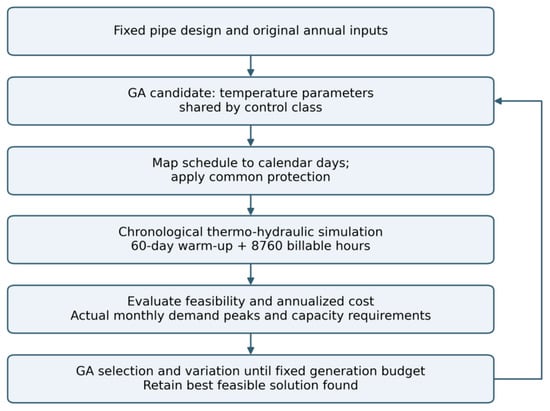
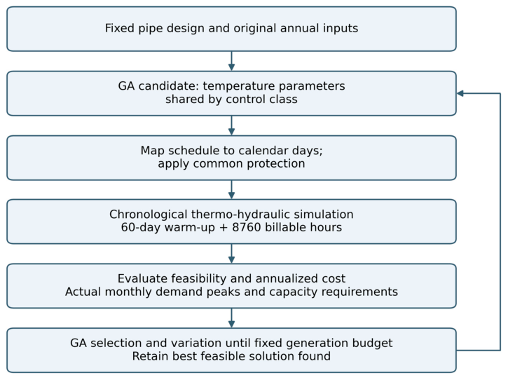
Because the optimization problem contains strong nonlinearities arising from the quadratic pressure-loss relation, temperature-dependent equipment performance, advective heat transport, changes in flow direction, and the representative-state iteration, together with discrete pipe-size decisions, a genetic algorithm is used because it does not require differentiability or convexity and can evaluate mixed discrete and continuous decisions through the nonlinear thermo-hydraulic model. The solution procedure is summarized in Figure 2.
Figure 2.
Genetic algorithm optimization with chronological annual thermo-hydraulic evaluation.
For each fixed pipe design, the genetic algorithm selects the station-temperature parameters for each control class. Each candidate schedule is mapped to the calendar year and evaluated using the original hourly loads, ground temperatures, and electricity prices. The embedded model calculates network flows, pipe-water and ground states, equipment and pumping electricity, physical constraint violations, and annualized cost.
The objective value and normalized constraint violations from the annual evaluation are returned to the genetic algorithm. Feasible candidates are ranked by annualized cost, whereas infeasible candidates are ranked by constraint violation. The search terminates at the prescribed generation limit; the retained result is the best feasible solution found within that budget. The optimization provides an idealized assessment of pipe-network thermal-storage potential under known weather and building loads.
2.10. Use of Generative AI
The authors used OpenAI Codex to generate the schematic of the modeled fifth-generation district heating and cooling system (Figure 1) and the flowchart of the genetic algorithm and annual thermo-hydraulic evaluation (Figure 2). The authors reviewed and edited the generated graphics to ensure that they accurately represented the system configuration and optimization procedure described in this section.
3. Case Study
3.1. Case Description and Input Data
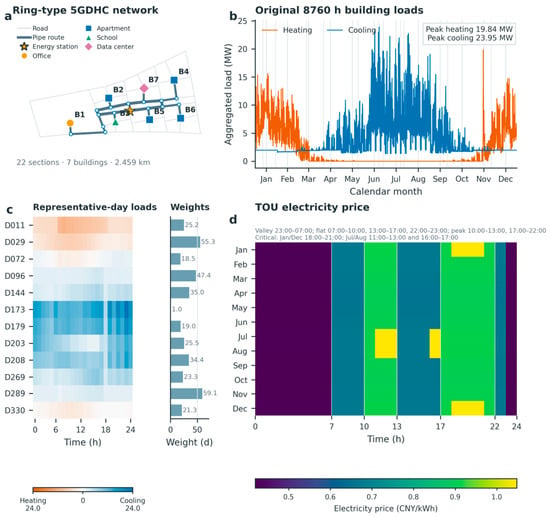
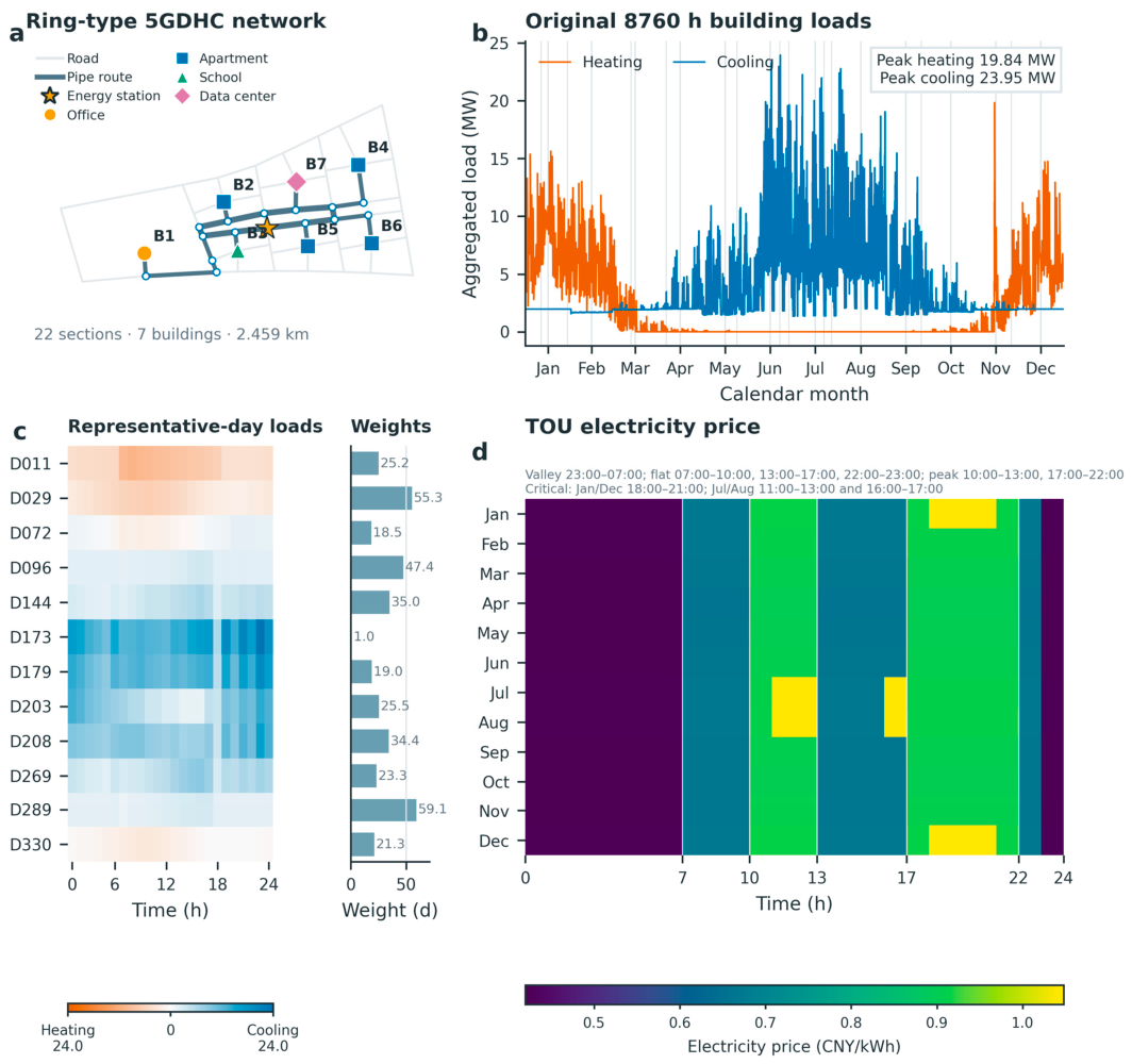
To evaluate the proposed optimization framework, a synthetic district based on our previous study [25] is considered. The district contains seven buildings: one medium office building, four mid-rise apartment buildings, one primary school, and one data center. Their heating and cooling loads were generated from EnergyPlus archetype simulations using Beijing weather data and were treated as fixed inputs to the optimization. Table 1 reports the peak heating and cooling loads of the individual buildings. The aggregated 8760 h load profiles reach peak heating and cooling demands of 19.84 and 23.95 MW, respectively (Figure 3b).
Table 1.
Peak heating and cooling loads of the individual buildings.
Figure 3.
Case-study inputs: (a) network layout, (b) annual heating and cooling loads, (c) representative days and weights, and (d) TOU electricity prices.
The building-side operating temperatures are determined by their end-use requirements. The heating supply and return temperatures are 45 and 35 °C, respectively. The cooling supply and return temperatures are 7 and 12 °C for all buildings except the data center, which operates at 16 and 30 °C. Cooling can be supplied directly through a heat exchanger when the cold-pipe temperature is sufficiently low. A minimum temperature difference of 2 K across the heat exchanger is imposed to account for its heat-transfer requirement.
A ring-type network was manually designed to connect the seven buildings and the central energy station, as shown in Figure 3a. The network contains 22 route sections with a total route length of 2.459 km. Each route section contains one warm pipe and one cold pipe with identical lengths and diameters. The network topology and route lengths remain fixed, whereas the pipe diameters are selected by the optimization model.
K-means clustering groups the 365 calendar days into 12 control classes using the daily heating and cooling profiles and ground-temperature information. Each centroid is represented by its nearest calendar day. The selected days and annual weights in Figure 3c and Table 2 describe this control parameterization; all candidates are evaluated using the original 8760 h inputs. A 24-class parameterization is examined as a sensitivity case.
Table 2.
Selected representative days and their annual weights.
Table 3 summarizes the principal physical and economic parameters applied to the case study. The warm- and cold-pipe temperatures at the central energy station are represented by their mean temperature and a fixed temperature difference of 7 K. The allowable mean-temperature range is therefore 5.5–31.5 °C, corresponding to the 2–35 °C limits imposed on the two station outlet temperatures. The same temperature limits are applied throughout the network. The hourly energy prices follow the TOU schedule shown in Figure 3d, while the maximum-demand charge is calculated separately.
Table 3.
Principal parameters applied to the case study.
The pipe-size data are adopted from our previous study [25]. The catalog contains 20 nominal diameters from DN50 to DN1400, with internal diameters ranging from 50 to 1388 mm. The corresponding unit costs range from 139 to 3134 CNY/m for one pipe. Because every route section contains one warm pipe and one cold pipe, the investment calculation includes the cost of both pipes. Table 4 provides the complete pipe-size catalog.
Table 4.
Pipe-size catalog used in the case study. Unit costs include civil works.
3.2. Experimental Design and Optimization Settings
This study evaluates the operational value of the existing network thermal capacity and the economic feasibility of increasing this capacity through pipe enlargement. For this purpose, six core cases are designed by combining two temperature-control strategies with three pipe-capacity levels. The temperature difference between the warm and cold pipes is fixed at 7 K in all core cases. This setting prevents changes in the mean network temperature and changes in the temperature difference from affecting the comparison simultaneously. The operational decision is therefore the mean-temperature trajectory at the central energy station.
The two temperature-control strategies are denoted Cases A and B. Under the daily-constant control adopted in Case A, one station mean temperature is optimized for each representative day and maintained for 24 h. This strategy can select a suitable operating temperature for each daily condition, but it cannot actively schedule the network thermal state by varying the station temperature within the day. Case B applies predictive control and allows the station mean temperature to vary within the day.
Directly optimizing the station temperature for every hour would introduce 24 temperature variables for each representative day and substantially increase the computational cost of the genetic algorithm with the embedded thermo-hydraulic model. Case B therefore optimizes six station mean-temperature points at 0, 4, 8, 12, 16, and 20 h. The hourly temperature trajectory is obtained through piecewise-linear interpolation between these points. This formulation reduces the number of temperature variables from 24 to six per cluster. The loads and electricity prices are used to determine the trajectory, allowing the water and surrounding soil to shift system electricity use over time.
The baseline pipe design was obtained under the daily-constant control of Case A using the thermo-hydraulic model and feasibility constraints described in Section 2. The resulting diameter vector defines the baseline pipe design, denoted k = 0.
After the baseline diameter vector is obtained, it is fixed and evaluated under both temperature-control strategies. Case A-k0 uses daily-constant control, whereas Case B-k0 applies predictive control to the same physical network. Two enlarged pipe designs are then constructed from the baseline design. For k = +1, the diameter of the warm and cold pipes in every route section is increased by one available catalog size. For k = +2, each diameter is increased by two catalog sizes. Cases A and B are reoptimized separately for each pipe-capacity level, producing the six core cases summarized in Table 5.
Table 5.
Core experiment design.
Cases A-k0 and B-k0 use identical pipes, building loads, station warm–cold temperature differences, and physical constraints. Their cost difference measures the incremental value of allowing the station mean temperature to vary within the day. This comparison includes both thermal-state scheduling and changes in temperature-dependent equipment performance.
Comparisons among k = 0, k = +1, and k = +2 under the same control strategy are used to evaluate the overall economic effect of pipe enlargement. Larger pipes increase the water volume and thermal capacity of the network while reducing hydraulic resistance. However, they require additional pipe investment. Pipe enlargement is economically justified only when the reductions in the other annualized cost components exceed the additional annualized pipe cost.
The benefits of pipe enlargement cannot be attributed entirely to the increase in thermal capacity. Even under daily-constant control, larger pipes may reduce pumping electricity, relieve hydraulic constraints, and allow the system to operate at a more favorable temperature. The cost difference between Cases A and B is therefore calculated separately at each pipe-capacity level. Comparing these differences indicates whether the additional water volume increases the marginal value of intraday temperature scheduling.
The six cases were optimized using pymoo 0.6.2, with a population of 24 and fixed limits of 15 generations for Case A and 25 generations for Case B. Simulated binary crossover used probability 0.9 and distribution index 15. Polynomial mutation used individual probability 0.9, distribution index 20, and variable probability min(0.5, 1/n), where n is the number of control variables. Feasibility-first ranking was applied. Matched pipe-design comparisons used common initial candidate pools and search budgets. Independent-seed repetitions were performed for the k0 and k + 1 predictive cases. With six parallel worker processes, recorded wall times, including final checks, were approximately 7.9–8.1 min for Case A and 13.3–17.5 min for Case B. Full settings, convergence histories, and repetitions are documented in Supplementary Materials.
3.3. Results Analysis
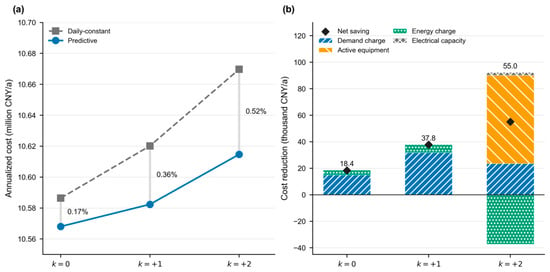
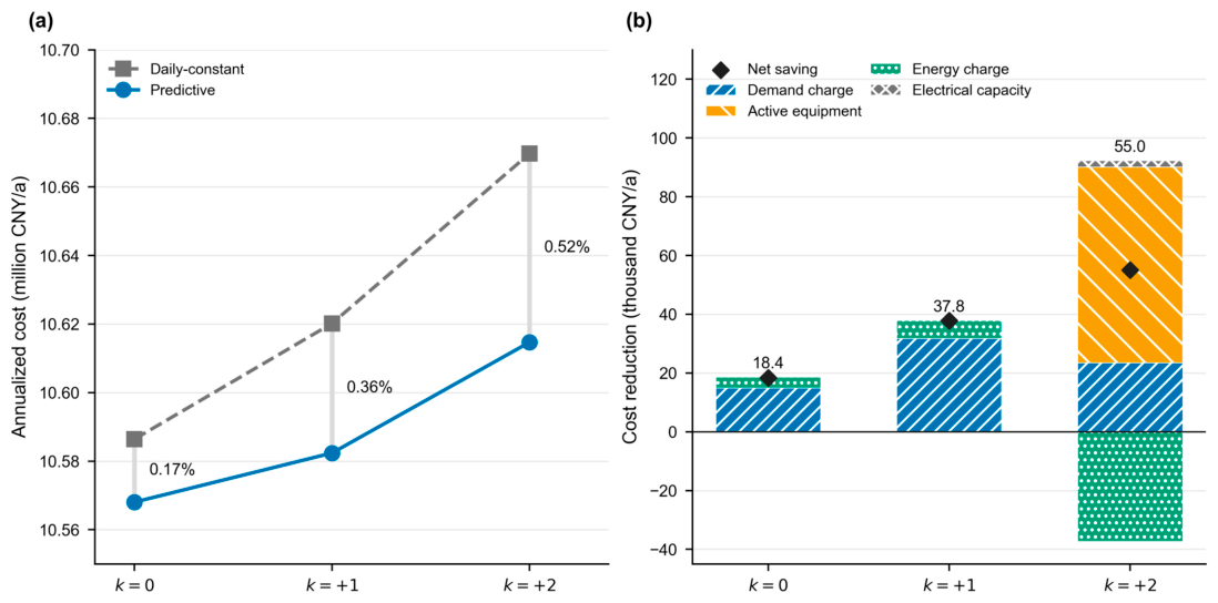
Predictive temperature control reduced the annualized cost at all three pipe-capacity levels, but the savings remained below 1% (Figure 4a). For the baseline network, the annualized cost decreased from 10.586 million CNY/a under daily-constant control to 10.568 million CNY/a under predictive control, corresponding to a saving of 18,400 CNY/a or 0.17%. The saving increased to 37,800 CNY/a at k = +1, equivalent to 0.36% of the daily-constant cost, and was 55,000 CNY/a at k = +2, equivalent to 0.52%. The largest reduction was therefore obtained at k = +2. Nevertheless, Predictive-k0 retained the lowest annualized cost among all six cases.
Figure 4.
Annualized cost and savings from predictive temperature control. (a) Annualized costs. (b) Savings by cost component.
The monthly demand charge was the main source of the savings from predictive control at k = 0 and k = +1 (Figure 4b). Its reduction contributed 14,900 and 31,800 CNY/a at k = 0 and k = +1, accounting for 81.0% and 84.1% of the corresponding net savings. By comparison, the energy charge decreased by 3800 and 6100 CNY/a at k = 0 and k = +1 and increased by 37,300 CNY/a at k = +2. The demand-charge savings at k = 0 and k = +1 came from lower monthly billing peaks; the annual maximum electrical demand increased by less than 0.3 kW in both cases. At k = +2, the active station-capacity reduction became the largest saving component: the required capacity decreased by 567.0 kW, saving 66,500 CNY/a. The economic value of predictive control was therefore governed mainly by monthly demand charges and active-equipment investment.
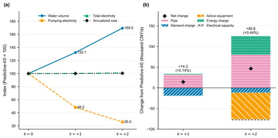
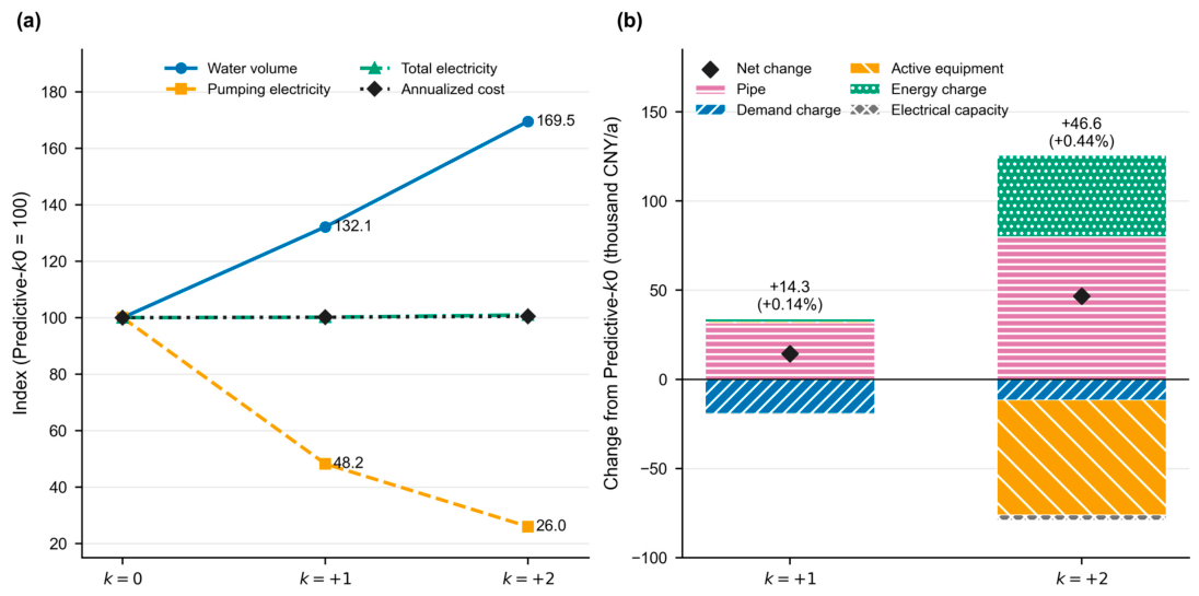
Increasing the pipe size substantially reduced pumping electricity but did not reduce the total annualized cost (Figure 5). Relative to Predictive-k0, the network water volume increased by 32.1% at k = +1 and by 69.5% at k = +2, while pumping electricity decreased from 15.50 MWh/a to 7.47 and 4.03 MWh/a, respectively. The corresponding total electricity consumption increased by 0.12% and 0.95%. The annualized cost consequently increased by 14,300 CNY/a at k = +1 and by 46,600 CNY/a at k = +2, equivalent to 0.14% and 0.44%. In the k = +2 case, the active station-capacity cost decreased by 64,400 CNY/a, but this saving and the 11,500 CNY/a reduction in monthly demand charge were insufficient to offset the increases of 80,000 CNY/a in pipe cost and 45,500 CNY/a in energy charge. Thus, the operating benefits provided by the enlarged pipes did not justify their additional investment in this district.
Figure 5.
Physical and economic effects of pipe enlargement under predictive control. (a) Water volume, electricity use, and cost. (b) Cost changes from k = 0.
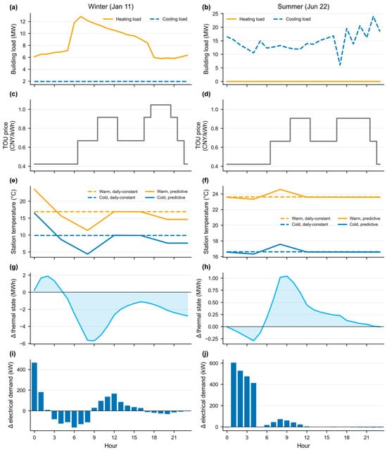
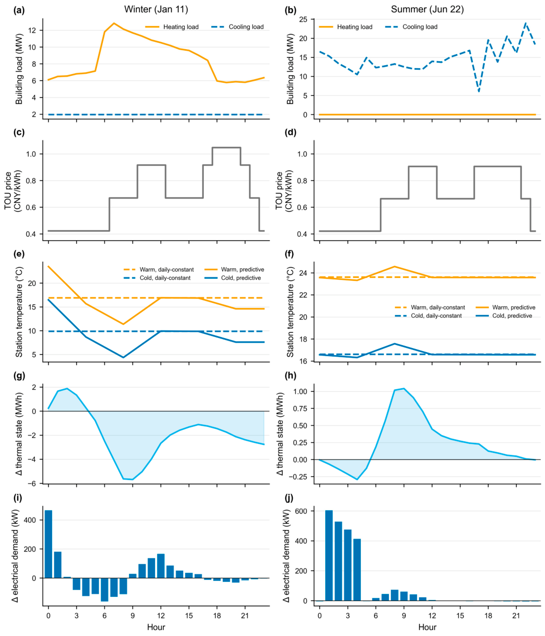
Figure 6 illustrates the operation of predictive control under winter and summer conditions. The k = +1 network is presented as the intermediate pipe design. On January 11, the heating load reached 12.84 MW at 7 h, while the data-center cooling load remained close to 1.97 MW. Predictive control lowered both station outlet temperatures by 4.45 K at 7 h. The network thermal state relative to daily-constant control fell from +1.88 MWh at 2 h to −5.62 MWh at 8 h, indicating heat release during the morning heating peak. The daily electrical peak decreased from 3.157 to 3.027 MW. Electrical demand was subsequently increased as the network thermal state was restored. On June 22, the district had only cooling demand, with a peak of 23.95 MW. The thermal-state difference ranged from −0.29 to +1.04 MWh, and the daily electrical peak decreased only slightly, from 2.966 to 2.961 MW. The winter trajectory therefore reduced the morning heating-related electrical peak, whereas the selected summer day showed a smaller electrical peak reduction. In both cases, the optimized temperature trajectory responded to the building loads, equipment performance, and capacity costs rather than simply following the TOU electricity price.
Figure 6.
Winter and summer operation of the k = +1 network. (a,b) Building loads. (c,d) TOU prices. (e,f) Station temperatures. (g,h) Δ thermal state. (i,j) Δ electrical demand. Δ denotes predictive minus daily-constant control.
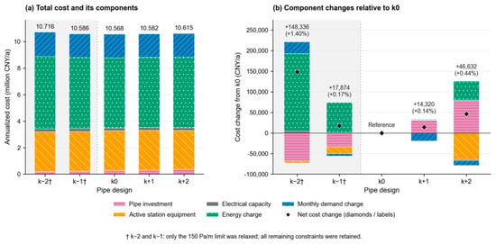
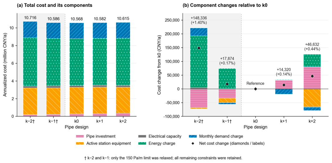
Figure 7 extends the predictive-control comparison from k − 2 to k + 2. The k − 1 and k − 2 designs exceeded the 150 Pa/m specific-friction limit specified in Table 3 and Equation (49). These two designs were therefore optimized with only this limit removed, while all remaining constraints were retained.
Figure 7.
Annualized cost decomposition across the five predictive-control pipe designs: (a) total cost and its components; (b) component changes relative to Predictive-k0. Black diamonds and labels indicate net cost changes. The specific-friction limit was relaxed only for k − 2 and k − 1; all other constraints were retained.
Across the five best solutions found, pipe investment accounted for 1.8–3.2% of total annualized cost, while energy and monthly demand charges together accounted for approximately 67–68%. Reducing pipe sizes lowered investment but increased energy charges. For the enlarged designs, net reductions in the other cost components offset only 54.7% and 41.7% of the additional pipe annuity at k + 1 and k + 2, respectively. The expanded comparison therefore showed limited economic justification for enlarging pipes specifically to increase thermal storage capacity in this case.
3.4. Sensitivity Analysis
To assess solution repeatability, the k0 and k + 1 predictive optimizations were repeated using different random seeds. Total annualized costs differed by only 0.18% and 0.24%, respectively, indicating consistent economic results across the repeated runs.
To examine the influence of the number of clusters, the predictive controls were optimized using 12 and 24 daily control classes. Total annualized costs differed by 1.57% at k0 and 1.70% at k + 1 (Section S2 of the Supplementary Materials). Although these changes exceeded the cost differences between pipe designs, both parameterizations showed limited economic separation between k0 and k + 1. Increasing the number of control classes did not reveal a substantial economic advantage for pipe enlargement.
Tariff sensitivity was examined by removing the monthly demand charge and by doubling the peak–off-peak spread while preserving the annual arithmetic mean price. Removing demand charges reduced total costs by approximately 17% but eliminated the demand-charge savings associated with pipe enlargement. Energy charges changed by only approximately 0.3% in both tariff scenarios. In the retained solutions, k + 1 remained 0.39% and 0.19% more expensive than k0, respectively. Thus, the tariff changes affected operating savings, but the incremental benefits of larger pipes remained insufficient to offset their additional investment. Detailed tariff sensitivity results are provided in Section S3 of the Supplementary Materials.
4. Discussion
For the investigated case, the results indicate that the existing pipe network can provide short-term operational flexibility, but its economic value is modest and depends mainly on avoided demand and capacity charges. The annualized cost reduction of 0.17–0.52% is consistent with the approximately 2% or lower cost savings reported for pipe-network storage in conventional district-heating systems [28,29]. This agreement suggests that, although the 5GDHC network in the present case can provide both heat- and cold-storage potential by adjusting the temperatures of its warm and cold pipes, this additional physical flexibility does not necessarily produce a large economic improvement.
The cost decomposition shows that predictive control generated most of its savings by reducing the monthly electrical demand and, at k = +2, the required central-station capacity, whereas the energy charge changed only slightly or increased. Shifting the network temperature affects heat-pump and chiller performance as well as heat transfer between the pipes and the ground. A reduction in peak demand can therefore be accompanied by a small increase in total electricity consumption. The economic value of pipe-network storage consequently depends more on the alignment among thermal loads, electrical peaks, and the tariff structure than on the available water volume alone.
This distinction is important when pipe enlargement is considered. In the tested designs, larger pipes increase the water volume and reduce pumping electricity, but they simultaneously increase pipe investment and alter the thermal and hydraulic operation of the network. Although the k = +2 design produced the largest relative saving from predictive control, it still had a higher annualized cost than the baseline pipe design. Additional network thermal capacity might become valuable when it can be dispatched frequently enough to reduce expensive electrical peaks and offset the additional pipe investment. From a design perspective, predictive temperature control should therefore be used to exploit the thermal capacity already available in the network before pipe enlargement is considered for the tested case.
5. Conclusions
This study developed a thermo-hydraulic optimization framework to evaluate the economic value of the thermal capacity available in a 5GDHC pipe network and determine whether increasing this capacity through pipe enlargement is economically justified. The framework represents the dynamic thermal behavior of the network together with its hydraulic operation, equipment performance, and economic costs. A genetic algorithm was adopted to solve the resulting nonlinear optimization problem. Daily-constant and predictive temperature control were compared at three pipe-capacity levels for a 5GDHC system in Beijing.
The results indicate that predictive temperature control reduced the annualized cost at all three pipe-capacity levels, but the savings remained between 0.17% and 0.52%. The monthly demand charge was the main source of these savings at the baseline and one-size-enlarged designs, while active-equipment investment was the largest saving component at the two-size-enlarged design, whereas the energy charge changed only slightly or increased. Increasing every pipe diameter by two catalogue sizes produced the largest saving from predictive control. Nevertheless, predictive control with the baseline pipe diameters retained the lowest annualized cost among the six main cases. Increasing every pipe diameter by one or two catalogue sizes increased the network water volume by 32.1% and 69.5% and reduced pumping electricity from 15.50 MWh/a to 7.47 and 4.03 MWh/a, respectively. However, the corresponding annualized costs increased by 14.3 and 46.6 thousand CNY/a (0.14% and 0.44%) relative to predictive control with the baseline pipe diameters. For the investigated case and tested pipe sizes, the results favor exploiting the existing network thermal capacity through temperature control before increasing pipe volume.
Because the investigated case represents a 5GDHC system in Beijing, both the magnitude of the economic benefits and the relative cost ranking of the tested pipe sizes may differ under other regional climates and operating conditions. The model further assumes a fixed station temperature difference between the warm and cold pipes. Future studies should evaluate pipe-network thermal storage in other climatic regions and investigate control strategies in which the temperature difference between the warm and cold pipes can vary, while accounting for weather and building-load forecast uncertainties during the operation. The demonstrated potential to reduce maximum electrical demand further suggests that 5GDHC pipe networks could be investigated as demand-side resources for electrical grid peak shaving.
Supplementary Materials
The following supporting information can be downloaded at: https://www.mdpi.com/article/10.3390/buildings16224569/s1, Figure S1: Pipe-water temperatures over a 24 h cycle; Figure S2: GA convergence for two random seeds; Table S1: Benchmark geometry, properties, and boundary conditions; Table S2: Hourly heat-transfer model errors; Table S3: Annualized costs with 12 and 24 control classes; Table S4: Annualized costs under alternative tariffs; Table S5: GA settings and random seeds; Table S6: GA run times and annualized costs; Table S7: Cost components and feasibility by pipe design. The supplementary file provides pipe–ground heat-transfer verification, control-class and tariff sensitivity results, optimization settings and convergence histories, and comparisons of smaller pipe designs.
Author Contributions
Conceptualization, L.S. and Y.Z.; methodology, L.S.; software, L.S.; validation, L.S. and S.L.; formal analysis, L.S.; investigation, L.S.; resources, S.L.; data curation, L.S.; writing—original draft preparation, L.S.; writing—review and editing, L.S., Y.Z. and S.L.; visualization, L.S.; supervision, Y.Z.; project administration, L.S. and Y.Z.; funding acquisition, L.S. All authors have read and agreed to the published version of the manuscript.
Funding
This work was supported by the Shanghai Pujiang Program under Grant No. 24PJA131 and by Anhui Province Key Laboratory of Intelligent Building and Building Energy Saving under Grant No. IBES2025KF13. The authors gratefully acknowledge the financial support provided through both grants.
Data Availability Statement
The data presented in this study are available on request from the corresponding author. The underlying input data are not publicly available due to data-sharing restrictions associated with a previous collaborative research project.
Acknowledgments
During the preparation of this manuscript, the authors used OpenAI Codex and Anthropic Claude for the purposes to improve the language, grammar, and clarity of the text and to generate the figures. The authors have reviewed and edited the output and take full responsibility for the content of this publication.
Conflicts of Interest
The author declares no conflicts of interest.
References
- United Nations Environment Programme; Global Alliance for Buildings and Construction. Global Status Report for Buildings and Construction: Beyond Foundations: Mainstreaming Sustainable Solutions to Cut Emissions from the Buildings Sector; United Nations Environment Programme: Nairobi, Kenya, 2024; Available online: https://wedocs.unep.org/handle/20.500.11822/45095 (accessed on 1 September 2026).
- Staffell, I.; Pfenninger, S.; Johnson, N. A Global Model of Hourly Space Heating and Cooling Demand at Multiple Spatial Scales. Nat. Energy 2023, 8, 1328–1344. [Google Scholar] [CrossRef] [Scilit]
- Mastrucci, A.; Boza-Kiss, B.; van Ruijven, B. Towards Net-Zero Emissions in Global Residential Heating and Cooling: A Global Scenario Analysis. Clim. Change 2025, 178, 85. [Google Scholar] [CrossRef] [Scilit]
- Lund, H.; Østergaard, P.A.; Nielsen, T.B.; Werner, S.; Thorsen, J.E.; Gudmundsson, O.; Arabkoohsar, A.; Mathiesen, B.V. Perspectives on Fourth and Fifth Generation District Heating. Energy 2021, 227, 120520. [Google Scholar] [CrossRef] [Scilit]
- Yao, S.; Wu, J.; Qadrdan, M. A State-of-the-Art Analysis and Perspectives on the 4th/5th Generation District Heating and Cooling Systems. Renew. Sustain. Energy Rev. 2024, 202, 114729. [Google Scholar] [CrossRef] [Scilit]
- Buffa, S.; Cozzini, M.; D’Antoni, M.; Baratieri, M.; Fedrizzi, R. 5th Generation District Heating and Cooling Systems: A Review of Existing Cases in Europe. Renew. Sustain. Energy Rev. 2019, 104, 504–522. [Google Scholar] [CrossRef] [Scilit]
- Wang, M.; Hu, E.; Chen, L. Simulation of a Radiation-Enhanced Thermal Diode Tank (RTDT) Assisted Refrigeration and Air-Conditioning (RAC) System Using TRNSYS. J. Build. Eng. 2024, 82, 108168. [Google Scholar] [CrossRef] [Scilit]
- Guelpa, E.; Verda, V. Thermal Energy Storage in District Heating and Cooling Systems: A Review. Appl. Energy 2019, 252, 113474. [Google Scholar] [CrossRef] [Scilit]
- Hennessy, J.; Li, H.; Wallin, F.; Thorin, E. Flexibility in Thermal Grids: A Review of Short-Term Storage in District Heating Distribution Networks. Energy Procedia 2019, 158, 2430–2434. [Google Scholar] [CrossRef] [Scilit]
- Vivian, J.; Quaggiotto, D.; Zarrella, A. Increasing the Energy Flexibility of Existing District Heating Networks Through Flow Rate Variations. Appl. Energy 2020, 275, 115411. [Google Scholar] [CrossRef] [Scilit]
- Van Oevelen, T.; Scapino, L.; Al Koussa, J.; Vanhoudt, D. A Case Study on Using District Heating Network Flexibility for Thermal Load Shifting. Energy Rep. 2021, 7, 1–8. [Google Scholar] [CrossRef] [Scilit]
- Gang, W.; Wang, S.; Xiao, F.; Gao, D.-C. District Cooling Systems: Technology Integration, System Optimization, Challenges and Opportunities for Applications. Renew. Sustain. Energy Rev. 2016, 53, 253–264. [Google Scholar] [CrossRef] [Scilit]
- Mazzoni, S.; Sze, J.Y.; Nastasi, B.; Ooi, S.; Desideri, U.; Romagnoli, A. A Techno-Economic Assessment on the Adoption of Latent Heat Thermal Energy Storage Systems for District Cooling Optimal Dispatch and Operations. Appl. Energy 2021, 289, 116646. [Google Scholar] [CrossRef] [Scilit]
- Wirtz, M.; Kivilip, L.; Remmen, P.; Müller, D. 5th Generation District Heating: A Novel Design Approach Based on Mathematical Optimization. Appl. Energy 2020, 260, 114158. [Google Scholar] [CrossRef] [Scilit]
- Maccarini, A.; Sotnikov, A.; Sommer, T.; Wetter, M.; Sulzer, M.; Afshari, A. Influence of Building Heat Distribution Temperatures on the Energy Performance and Sizing of 5th Generation District Heating and Cooling Networks. Energy 2023, 275, 127457. [Google Scholar] [CrossRef] [Scilit]
- Mans, M.; Blacha, T.; Schreiber, T.; Müller, D. Development and Application of an Open-Source Framework for Automated Thermal Network Generation and Simulations in Modelica. Energies 2022, 15, 4372. [Google Scholar] [CrossRef] [Scilit]
- Pompei, L.; Nardecchia, F.; Miliozzi, A.; Groppi, D.; Astiaso Garcia, D.; De Santoli, L. Assessment of the Optimal Energy Generation and Storage Systems to Feed a District Heating Network. Buildings 2024, 14, 2370. [Google Scholar] [CrossRef] [Scilit]
- Elhafaia, M.H.; Nova-Rincon, A.; Sochard, S.; Serra, S.; Reneaume, J.-M. Optimization of the Pipe Diameters and the Dynamic Operation of a District Heating Network Using a Robust Initialization Strategy. Appl. Therm. Eng. 2025, 258, 124533. [Google Scholar] [CrossRef] [Scilit]
- Zhang, Y.; Liu, M.; O’Neill, Z.; Wen, J. Temperature Control Strategies for Fifth Generation District Heating and Cooling Systems: A Review and Case Study. Appl. Energy 2024, 376, 124156. [Google Scholar] [CrossRef] [Scilit]
- Dai, J.; Ikeda, S.; Ooka, R. Control Strategies in Fifth-Generation District Heating and Cooling Systems: A Review. Sustain. Cities Soc. 2026, 148, 107690. [Google Scholar] [CrossRef] [Scilit]
- Wirtz, M.; Neumaier, L.; Remmen, P.; Müller, D. Temperature Control in 5th Generation District Heating and Cooling Networks: An MILP-Based Operation Optimization. Appl. Energy 2021, 288, 116608. [Google Scholar] [CrossRef] [Scilit]
- Buffa, S.; Soppelsa, A.; Pipiciello, M.; Henze, G.; Fedrizzi, R. Fifth-Generation District Heating and Cooling Substations: Demand Response with Artificial Neural Network-Based Model Predictive Control. Energies 2020, 13, 4339. [Google Scholar] [CrossRef] [Scilit]
- Quirosa, G.; Torres, M.; Soltero, V.M.; Chacartegui, R. Analysis of an Ultra-Low Temperature District Heating and Cooling As a Storage System for Renewable Integration. Appl. Therm. Eng. 2022, 216, 119052. [Google Scholar] [CrossRef] [Scilit]
- Ho, C.-O.; Nie, T.; Su, L.; Yang, Z.; Schwegler, B.; Calvez, P. Graph-Based Algorithmic Design and Decision-Making Framework for District Heating and Cooling Plant Positioning and Network Planning. Adv. Eng. Inform. 2021, 50, 101420. [Google Scholar] [CrossRef] [Scilit]
- Su, L.; Nie, T.; Ho, C.O.; Yang, Z.; Calvez, P.; Jain, R.K.; Schwegler, B. Optimizing Pipe Network Design and Central Plant Positioning of District Heating and Cooling System: A Graph-Based Multi-Objective Genetic Algorithm Approach. Appl. Energy 2022, 325, 119844. [Google Scholar] [CrossRef] [Scilit]
- Su, L.; Yang, Z.; Jain, R.K. Design and Investment Strategy Optimization of District Cooling System During the Ramp-Up Phase. Energy Build. 2024, 321, 114603. [Google Scholar] [CrossRef] [Scilit]
- Jensen, J.K.; Ommen, T.; Reinholdt, L.; Markussen, W.B.; Elmegaard, B. Heat pump COP, part 2: Generalized COP Estimation of Heat Pump Processes. In Proceedings of the 13th IIR Gustav Lorentzen Conference on Natural Refrigerants; International Institute of Refrigeration: Paris, France, 2018; Volume 2, pp. 1136–1145. [Google Scholar] [CrossRef]
- Kouhia, M.; Laukkanen, T.; Holmberg, H.; Ahtila, P. District Heat Network as a Short-Term Energy Storage. Energy 2019, 177, 293–303. [Google Scholar] [CrossRef] [Scilit]
- Zhang, Y.; Johansson, P.; Sasic Kalagasidis, A. Feasibilities of Utilizing Thermal Inertia of District Heating Networks to Improve System Flexibility. Appl. Therm. Eng. 2022, 213, 118813. [Google Scholar] [CrossRef] [Scilit]

Disclaimer/Publisher’s Note: The statements, opinions and data contained in all publications are solely those of the individual author(s) and contributor(s) and not of MDPI and/or the editor(s). MDPI and/or the editor(s) disclaim responsibility for any injury to people or property resulting from any ideas, methods, instructions or products referred to in the content. |
© 2026 by the authors. Licensee MDPI, Basel, Switzerland. This article is an open access article distributed under the terms and conditions of the Creative Commons Attribution (CC BY) license.